Correction of the Lusztig-Williamson Billiards Conjecture

Abstract

A new algorithm allows us to calculate many new tilting characters for $SL_{3}$, $SP_{4}$, $G_{2}$, $SL_{4}$ and potentially many other groups. These calculations show that the Lusztig-Williamson Billiards Conjecture needs to be corrected. In this paper we present the new results calculated for $SL_{3}$ and a correction of the conjecture.

1 Introduction

Recent results show that the characters of indecomposable tilting modules of reductive algebraic groups in characteristic $p$ are given by the $p$-Kazhdan-Lusztig basis of the corresponding anti-spherical module (see [RW18, AMRW19, RW20, BR20]) for all primes $p$. In joint work with Geordie Williamson, the author has developed and implemented (in Magma, see [BCP97]) a new algorithm to calculate the $p$-Kazhdan-Lusztig basis of the anti-spherical module. This algorithm will be described in detail in a separate paper. Even though the calculations which the paper [LW18] is based on can now be carried out in less than 24 hours, this should not be considered a full solution to the problem.

The Lusztig-Williamson Billiards Conjecture gives a combinatorial description of second generation tilting characters for $SL_{3}$ in terms of billiard balls bouncing around in the $p$-alcove geometry of the dominant cone. For background on the generational philosophy we refer the reader to [LW18, §2] and the references therein. The new calculations show that the Lusztig-Williamson Billiards Conjecture actually predicts second generation tilting characters that are “too big” and thus needs to be corrected. We propose a correction to the conjecture that is coherent with all the data we can currently calculate for $SL_{3}$.

1.1 Structure of the Paper

Section 2

We will fix important notation and recall generations for the $p$-Kazhdan-Lusztig basis of the anti-spherical module.

Section 3

In this section, we will explain the correction to the Lusztig-Williamson Billiards Conjecture. The reader will understand why the original conjecture predicts anti-spherical $p$-Kazhdan-Lusztig basis elements that are “too big”.

Section 4

Finally, we will explain how to obtain the figures from the anti-spherical $p$-Kazhdan-Lusztig basis calculated by our algorithm and mention all the examples for the newly proposed merging rule that can be found in the current data.

1.2 Acknowledgements

The counterexample to the Lusztig-Williamson Billiards Conjecture was discovered while the author was trying to understand the combinatorics of the Smith-Treumann localization of the anti-spherical module during a research at the Sydney Mathematical Research Institute. For that reason, the author would like to thank Geordie Williamson for the invitation and the SMRI for the excellent working conditions. In addition, the author would like to thank Allan Steel for helping to improve the runtime of the algorithm. During that period the author has received funding from the European Research Council (ERC) under the European Union’s Horizon 2020 research and innovation programme (grant agreement No 677147).

2 Notation

Let $G$ be a split simple and simply connected algebraic group over an algebraically closed field of characteristic $p$ and fix a Borel subgroup together with a maximal torus $T\subseteq B\subseteq G$. We will imitate the notation of [LW18, §2] to make the transition between the two papers as easy as possible for the reader:

$$\mathscr{X},\mathscr{X}_{+},\mathscr{X}_{++}\text{:}\quad$$ weights, dominant weights, strictly dominant weights;

$$\Phi,\Phi_{+}\text{:}\quad$$ roots, positive roots;

$$\Sigma\text{:}\quad$$ simple roots;

$$\rho,\alpha_{0}^{\vee}\text{:}\quad \Phi_{+}$$ half-sum of , highest short coroot;

$$W_{\text{f}},W\text{:}\quad$$ finite Weyl group, affine Weyl group;

$$S_{\text{f}},S\text{:}\quad$$ finite simple reflections, affine simple reflections;

$${}^{\text{f}}W\text{:}\quad W_{\text{f}}\backslash W$$ minimal coset representatives for the cosets ;

$$\cdot_{p},h\text{:}\quad p W \mathscr{X}$$ -dilated dot action of on , Coxeter number.

Let $H$ (resp. $H_{\text{f}}$) be the Iwahori-Hecke algebra of the affine (resp. finite) Weyl group $W$ (resp. $W_{\text{f}}$) over $\mathbb{Z}[v,v^{-1}]$ and consider the anti-spherical module:

$$AS_{v}\coloneqq\operatorname{sgn}_{v}\otimes_{H_{\text{f}}}H=\bigoplus_{x\in{}^{\text{f}}W}\mathbb{Z}[v,v^{-1}]n_{x}$$

The anti-spherical module has a Kazhdan-Lusztig basis $\{\underline{n}_{x}\;|\;x\in{}^{\text{f}}W\}$ and a $p$-Kazhdan-Lusztig basis $\{\prescript{p}{}{\underline{n}}_{x}\;|\;x\in{}^{\text{f}}W\}$. Lusztig and Williamson expect that for all $p>h$ and $x\in{}^{\text{f}}W$ there exist elements $\prescript{p}{}{\underline{n}}^{1}_{x}$, $\prescript{p}{}{\underline{n}}^{2}_{x}$, $\dots$, $\prescript{p}{}{\underline{n}}^{\infty}_{x}\in AS_{v}$ (see [LW18, §2.4]) such that:

1. $\prescript{p}{}{\underline{n}}^{1}_{x}=\underline{n}_{x}$;

2. $\prescript{p}{}{\underline{n}}^{\infty}_{x}=\prescript{p}{}{\underline{n}}_{x}$;

3. $\prescript{p}{}{\underline{n}}^{n}_{x}$ is a $\mathbb{Z}_{\geqslant 0}[v,v^{-1}]$-linear combination of $\{\prescript{p}{}{\underline{n}}^{n-1}_{y}\;|\;y\in{}^{\text{f}}W\}$ for all $n\geqslant 1$;

4. if $\langle\alpha_{0}^{\vee},x\cdot_{p}0+\rho\rangle\leqslant p^{n+1}$ then $\prescript{p}{}{\underline{n}}^{n}_{x}=\prescript{p}{}{\underline{n}}^{n+1}_{x}=\dots=\prescript{p}{}{\underline{n}}^{\infty}_{x}$.

This expectation was motivated by the generational philosophy and based on the hypothesis that the tilting character generations can be lifted to the non-trivial grading of the category of tilting modules given by the anti-spherical category (see [RW18, Theorem 5.3]).

3 The Corrected Conjecture

The Lusztig-Williamson Billiards Conjecture gives a combinatorial description of $\{\prescript{p}{}{\underline{n}}^{2}_{x}\;|\;x\in{}^{\text{f}}W\}$ for $G=SL_{3}$. For that reason, we will fix $G=SL_{3}$ for the rest of the paper. Thus, we have $\mathscr{X}=\mathbb{Z}\varpi_{1}\oplus\mathbb{Z}\varpi_{2}$, $\mathscr{X}_{+}\coloneqq\mathbb{Z}_{\geqslant 0}\varpi_{1}\oplus\mathbb{Z}_{\geqslant 0}\varpi_{2}$ $\mathscr{X}_{++}\coloneqq\mathbb{Z}_{>0}\varpi_{1}\oplus\mathbb{Z}_{>0}\varpi_{2}$, etc..

Fix $\ell\leqslant 3$. Note that $\ell$ will be prime for the representation theoretic applications. Denote by $\mathcal{M}\coloneqq\mathbb{Z}_{\geqslant 0}\times\{v^{k}\;|\;k\in\mathbb{Z}\}$ the set of labels. The element $(m,v^{k})\in\mathcal{M}$ will be written as $m(v^{k})$. A labelled point is an element of $\mathscr{X}\times\mathcal{M}$. Throughout this section all set-theoretic operations (i.e. unions, differences, …) should be understood in the context of multisets (i.e. sets with multiplicities).

In [LW18, §4] Lusztig-Williamson describe an algorithm which in three steps produces a multiset $\widetilde{Z}$ from which one can conjecturally obtain the set $\{\prescript{p}{}{\underline{n}}^{2}_{x_{i}}\;|\;i\geqslant 0\}$ where

$$x_{0}\coloneqq\mathrm{id}\text{, }x_{1}\coloneqq s_{0}\text{, }x_{2}\coloneqq s_{0}s_{1}\text{, }x_{3}\coloneqq s_{0}s_{1}s_{2}\text{, }x_{4}\coloneqq s_{0}s_{1}s_{2}s_{0},\dots$$

and $\{s_{0}\}=S\setminus S_{\text{f}}$ is the affine reflection.

In the correction, the first and the third step of the algorithm remain unchanged and we refer the reader to [LW18, §4.2 and §4.4] for their description. The first step starts with the labelled point $(0,0(v^{0}))$ and produces a set $X$ by extending along a wall of the dominant cone in the direction of $\varpi_{1}$. In each step, certain labelled points are designated as seeds and serve as input for the next step. The seeds in $X$ are the labelled points of the form $(k\ell\varpi_{1},2k\ell(v^{0}))$ for $k\geqslant 1$.

Before we explain the correction of the second step, we should mention how to put everything together in the end. The third step of the algorithm takes the multiset $Y$ produced by the second step and extends it within the interior of each $\ell$-alcove to produce a multiset $Z$. Finally, we set $\widetilde{Z}\coloneqq Z\setminus X$.

In order to formulate the conjecture, we will need some more notation from [LW18, §6]. Recall our prime $p$ from Section 2 and consider the multiset $\widetilde{Z}$ defined as above for $\ell=p$. Consider the $\mathbb{Z}$-linear map $\varphi:\mathbb{Z}[v]\rightarrow\mathbb{Z}[v,v^{-1}]$ defined via $v^{0}\mapsto 1$ and $v^{k}\mapsto v^{k}+v^{-k}$ for $k>0$. For an element $w\in W$ we will denote by $\mathcal{R}(w)\coloneqq\{s\in S\;|\;ws<w\}$ its right descent set. Fix the fundamental alcove

$$\mathcal{A}_{0}\coloneqq\{\lambda\in\mathscr{X}\otimes_{\mathbb{Z}}\mathbb{R}\;|\;0<\langle\alpha^{\vee},\lambda\rangle<1\text{ for all }\alpha\in\Phi_{+}\}$$

and recall the action of $W$ on the set of alcoves induced by the continuous action of $W$ on $\mathscr{X}\otimes_{\mathbb{Z}}\mathbb{R}$. As described in [LW18, §6], for $\mu\in\mathscr{X}_{++}$ and $s\in S$ there exists a unique element $x_{\mu}^{s}\in{}^{\text{f}}W$ such that $s\in\mathcal{R}(x_{\mu}^{s})$ and the open box

$$B_{\mu}\coloneqq\{\lambda\in\mathscr{X}\otimes_{\mathbb{Z}}\mathbb{R}\;|\;\langle\alpha^{\vee},\mu\rangle<\langle\alpha^{\vee},\lambda\rangle<\langle\alpha^{\vee},\mu\rangle+1\text{ for all }\alpha\in\Sigma\}$$

contains the alcove $x\mathcal{A}_{0}$.

Define ${}^{p}\zeta_{0}\coloneqq\underline{n}_{x_{0}}$. For $i>0$ let $s$ be the unique simple reflection in $\mathcal{R}(x_{i})$ and define the element

$${}^{p}\zeta_{i}\coloneqq\underline{n}_{x_{i}}+\sum_{\begin{subarray}{c}(\mu,n(v^{k}))\in\widetilde{Z}\\ n\in\{i,i-1,i-2\}\end{subarray}}\varphi(v^{k})\underline{n}_{x_{\mu}^{s}}\text{.}$$

Conjecture 3.1 (Corrected Lusztig-Williamson Billiards Conjecture).

We have:

1. ${}^{p}\zeta_{i}=\prescript{p}{}{\underline{n}}_{x_{i}}$ for $0\leqslant i<2p(p+1)$,

2. ${}^{p}\zeta_{i}=\prescript{p}{}{\underline{n}}^{2}_{x_{i}}$ for all $0\leqslant i$.

3.1 Corrected 2. Step: Dynamics on the Walls

In order to describe the second step of the algorithm, we first need to recall some definitions from [LW18, §4.3] and we will refer the reader to the original source for some beautiful illustrations of these definitions.

Corner points are points $\lambda\in\mathscr{X}_{+}$ such that $\langle\lambda,\alpha^{\vee}\rangle\in\ell\mathbb{Z}$ for all $\alpha\in\Phi_{+}$. Consider the directed graph $\Gamma$ on the vertex set $\mathscr{X}_{+}$ with edges $\lambda\rightarrow\lambda+\gamma$ for $\lambda,\lambda+\gamma\in\mathscr{X}_{+}$ and $\gamma\in\{\varpi_{1},\varpi_{2}-\varpi_{1},-\varpi_{2}\}$. A point $\mu\in\mathscr{X}_{+}$ is called an almost corner if there exists a corner point $\lambda\in\mathscr{X}_{+}$ and an edge $\lambda\rightarrow\mu$ in $\Gamma$.

For the dynamics on the walls, the following subgraphs $\Gamma_{\text{wall}}$ and $\Gamma_{\ell}$ of $\Gamma$ will be important. The vertex set of $\Gamma_{\ell}$ consists of weights $\lambda\in\mathscr{X}_{+}$ such that $\langle\lambda,\alpha^{\vee}\rangle\in\ell\mathbb{Z}$ for some $\alpha\in\Phi_{+}$. The only edges in $\Gamma_{\ell}$ are those $\lambda\rightarrow\lambda^{\prime}$ where $\langle\lambda,\alpha^{\vee}\rangle=\langle\lambda^{\prime},\alpha^{\vee}\rangle\in\ell\mathbb{Z}$ for some $\alpha\in\mathscr{X}_{+}$. Define $\Gamma_{\text{wall}}$ to be the induced subgraph of $\Gamma_{\ell}$ where we remove all the vertices that lie along the walls of the dominant cone except for $\{k\ell\varpi_{1},k\ell\varpi_{2}\;|\;k\geqslant 1\}$. Recall that the labelled points of the form $(k\ell\varpi_{1},2k\ell(v^{0}))$ are designated as seeds in the first step of the algorithm.

Fix a labelled point $(\mu,n(v^{k}))$ with $\mu\in\Gamma_{\text{wall}}$ such that there is a unique edge with source $\mu$ in $\Gamma_{\text{wall}}$. First, Lusztig and Williamson define three elementary operations to obtain labelled points in $\Gamma_{\text{wall}}\times\mathcal{M}$:

1. A rest gives the labelled point $(\mu,(n+3)(v^{k+1}))$.

2. A small step gives the labelled point $(\mu^{\prime},(n+2)(v^{k}))$ where $\mu\rightarrow\mu^{\prime}$ is the unique edge in $\Gamma_{\text{wall}}$ starting in $\mu$.

3. If $\mu$ is neither a corner nor an almost corner point, a giant leap gives either one or two new labelled points as follows: Let $d$ be the direction of the unique arrow in $\Gamma_{\text{wall}}$ starting in $\mu$. First take $j<\ell-1$ steps in the graph $\Gamma_{\text{wall}}$ in direction $d$ until we reach a corner point, say $\lambda$. Then continue with another $\ell-1-j$ steps in all directions different from $d$ from $\lambda$. (There are either one or two such directions depending on whether we are close to the walls of the dominant cone or not.) The giant leap consists of the resulting points labelled by $(n+2\ell+1)(v^{k+1})$. In the following we will also call this a giant leap towards $\lambda$.

Then they define one iteration of the algorithm producing a multiset of elements in $\Gamma_{\text{wall}}\times\mathcal{M}$. Some of these labelled points will be designed as seeds and thus serve as input for the third step of the algorithm. Using the fixed labelled point $(\mu,n(v^{k}))$ as input, we proceed as follows:

1. If $\mu$ is a corner point, then $\ell$ new labelled points are obtained by taking $\ell-1$ small steps to obtain $m_{1},m_{2},\dots,m_{\ell-1}$ and then a rest to produce $m_{\ell}$. The last labelled point $m_{\ell}$ is designated as a seed. This operation is called resting once.

2. If $\mu$ is an almost corner point, then $\ell$ new labelled points are obtained by taking first a rest to produce $m_{1}$, then $\ell-2$ small steps to obtain $m_{2},\dots m_{\ell-1}$ and finally another rest to produce $m_{\ell}$. The last labelled point $m_{\ell}$ is designated as a seed. We will call this operation resting twice.

3. If $\mu$ is neither a corner nor an almost corner point, then we take a giant leap to produce one or to new labelled points, each of which are designated as seeds.

Given a seed $q_{k}=(k\ell\varpi_{1},2k\ell(v^{0}))$ in $X$ for some $k\geqslant 1$, we iterate this process as follows: Starting with $Q_{0}\coloneqq\{q_{k}\}$ we obtain a sequence of multisets $Q_{1},Q_{2},\dots$ where $Q_{i}$ is the multiset obtained by taking the union of the outputs of the above procedure applied to each seed in $Q_{i-1}$ and then applying the following geometric merge rule for every corner point $\lambda$:

Merge Rule.

If giant leaps towards $\lambda$ lead to a superposition of labelled points (i.e. at least one labelled point occuring with multiplicity two), then among the seeds produced by these giant leaps towards $\lambda$ we only keep the superposed seeds and reduce their multiplicity to one.

Finally we say that the union $Y_{k}=\bigcup_{i\geqslant 1}Q_{i}$ is the result of applying dynamics on the walls to $q_{k}$. Note that the geometric merge rule is the only new ingredient in the correction.

The output of the corrected second step is given by the multiset

$$Y\coloneqq X\cup\bigcup_{k\geqslant 1}Y_{k}$$

together with the information which elements of $Y$ are designated as seeds.

In order to make the geometric merge rule more explicit, we want to explain the three possible cases for every corner point $\lambda$:

1. If there is one giant leap towards $\lambda$, it produces one or two labelled points (depending on whether $\lambda$ is close to the walls of the dominant cone or not).

2. If there are two giant leaps towards $\lambda$, they produce one labelled point (where the coefficient is half the sum of the superposed coefficients). We will call this case merging of type 2 around $\lambda$.

3. If there are three giant leaps towards $\lambda$, they produce three labelled points (each with half the sum of the superposed coefficients as coefficient). This case is called merging of type 3 around $\lambda$.

(a) of type 2

(b) of type 3

Figure 1: Examples of Merging for $\ell=5$

Remark 3.2.

1. Lusztig and Williamson were not aware of the merging phenomenon as they did not have a single occurrence of it in the data they could calculate.

2. The merge rule annihilates [LW18, Remark 4.3]. In other words, it prevents exponentially growing coefficients and thus the corrected conjecture no longer implies that decomposition numbers for symmetric groups display exponential growth.

3.2 A Larger Example and Some Observations

Figures 3 and 3 show larger examples to illustrate the geometric merge rule. They show for $\ell=5$ the multiset after the first ten iterations of the algorithm described in the second step applied to the seeds $(k\ell\varpi_{1},2k\ell(v^{0}))$ for $k\in\{1,2\}$. In this example, we have underlined all seeds and used the colours red (resp. blue) to mark seeds that arise from a merging of type 3 (resp. of type 2). When looking at this example the reader should observe the following:

• All the seeds in $Q_{j}$ are obtained by applying the same type of operation to some seed in $Q_{j-1}$. Looking at this operation for the sequence of multisets $Q_{1},Q_{2},Q_{3},\dots$, we get the following $\ell$-periodic pattern of operations:

  $$\text{resting once, }\underbrace{\text{giant leap, \ldots, giant leap}}_{(\ell-2)\text{-times}}\text{, resting twice,}$$

  $$\overline{\underbrace{\text{giant leap, \ldots, giant leap}}_{(\ell-1)\text{-times}}\text{, resting twice}}\text{, \ldots}$$

• There are no seeds with a label $n(v^{k\ell})$ for $n\in\mathbb{N}$ and $k\geqslant 1$ (simply because resting twice augments the exponent of $v$ by $2$ whereas all other operations increase it by $1$).

• For a labelled point $(\mu,n(v^{k}))\in\Gamma_{\text{wall}}\times\mathcal{M}$ we always have:

  $$n\equiv k\mod\ell$$

• For a labelled point $(\mu,n(v^{k}))\in\Gamma_{\text{wall}}\times\mathcal{M}$, the residue of $n$ modulo $\ell$ determines the position of the labelled point along the wall on which it lies.

• The seeds in $Q_{j}$ obtained from any seed in $X$ are all of the form

  $$(\mu,n(v^{j+\lfloor\frac{j-1}{\ell-1}\rfloor}))$$

  for various $\mu\in\mathscr{X}_{+}$. In other words, the exponent of $v$ determines how many iterations are needed to produce this point.

• The previous observations together imply that there are no superposition of labelled points in $Y_{j}$ and $Y_{k}$ for $j\neq k$.

• All labelled points $(\mu,n(v^{k}))$ lying in $Y_{k}$ (i.e. the ones obtained by applying the iterative algorithm in the second step to $(k\ell\varpi_{1},2k\ell(v^{0}))$) satisfy $\mu=a\varpi_{1}+b\varpi_{2}$ with

  $$0<a<k\ell\quad\text{ and }\quad 0<b\text{.}$$

  In other words, they lie in the first $k$ “columns” of the dominant cone (see Figures 3 and 3).

• The keen reader might have noticed that the “column” depicted in Figure 3 matches up to the global label shift $n(v^{k})\mapsto(n+10)(v^{k})$ the second “column” in Figure 3 (without the left wall!). More generally, the mapping $Y_{j}\rightarrow Y_{k}$ for $j<k$ given by $(\mu,n(v^{i}))\mapsto(\mu+(k-j)\ell\varpi_{1},(n+2(k-j)\ell)(v^{i}))$ is well-defined, injective and surjective onto the set

  $$\{(a\varpi_{1},+b\varpi_{2},n(v^{i}))\in Y_{k}\;|\;(k-j)\ell<a\}\text{.}$$

  This suggests a striking self-similarity of the data! Moreover, it implies that for the second step it is enough to understand the combinatorics of the wall dynamics applied to the seed $(k\ell\varpi_{1},2k\ell(v^{0}))$ in the limit for $k\rightarrow\infty$. From this, one can obtain the multiset $Y$ by taking unions of preimages of various maps of the type described above.

Figure 2: $(5\varpi_{1},10(v^{0}))$

Figure 3: $(10\varpi_{1},20(v^{0}))$

These figures show the multiset for $\ell=5$ after the first $10$ iterations applied to

4 The current Data

The current data for $\ell=3$, $\ell=5$, $\ell=7$ and $\ell=11$ is displayed in four figures at the end of the paper.

4.1 Preparation of the Data

Imagine we have calculated the elements $\prescript{p}{}{\underline{n}}_{x_{i}}$ for $1\leqslant i\leqslant n$. In this section we will explain how we have obtained the figures at the end of the paper from the given data. We have applied the following steps to process the data:

1. Express the elements $\prescript{p}{}{\underline{n}}_{x_{i}}$ for $1\leqslant i\leqslant n$ in terms of the Kazhdan-Lusztig basis $\{\underline{n}_{x}\;|\;x\in{}^{\text{f}}W\}$ of the anti-spherical module.

2. Illustrate all calculated $p$-Kazhdan-Lusztig basis elements in one combined picture as follows: For a Laurent polynomial $f$ let $\bar{f}$ be the polynomial obtained by forgetting all negative powers of $v$ and their coefficients in $f$. If $\underline{n}_{y}$ occurs with coefficient $f$ in $\prescript{p}{}{\underline{n}}_{x_{j}}$, then write $j(\bar{f})$ in the $p$-alcove corresponding to $y$.

3. For all $\mu\in\mathscr{X}_{++}$ replace each “triple” of the form

   by

   .

   These triples are consequences of the Kazhdan-Lusztig star operations as follows: Denote the simple reflections as $s\coloneqq x_{i}^{-1}x_{i+1}$, $t\coloneqq x_{i+1}^{-1}x_{i+2}$ and $u\coloneqq x_{i+2}^{-1}x_{i+3}$. Observe that the wall separating the two $p$-alcoves in the box $B_{\mu}$ will be $s$-coloured. So one may apply [Jen20, Proposition 4.5] first to the two rank $2$ standard parabolic subgroup given by $\{s,u\}$ and then to $\{s,t\}$ to obtain the triple shown above.

The resulting figures are depicted at the end of the paper.

It should be noted that in order to compare the figures with the predictions of the conjecture, the reader still needs to use the following heuristic to remove third generation phenomena. Even though there is no precise definition of $\{\prescript{p}{}{\underline{n}}^{3}_{x}\;|\;x\in{}^{\text{f}}W\}$ in general, we have a clear understanding of what it is for $SL_{2}$ (see explanation and Figure 4 below).

Heuristic.

Remove any labelled point $(\mu,n(v^{k}))$ (and all labelled points induced by it) whose restriction to a rank $1$ Levi subgroup gives a third generation contribution.

For $SL_{2}$ the affine Weyl group is isomorphic to the infinite dihedral group

$$W=\langle s,t\;|\;s^{2}=t^{2}=\mathrm{id}\rangle\text{.}$$

Let ${}_{s}\hat{k}$ denote the alternating word in $s$ and $t$ of length $k$ starting in $s$. Suppose that $t$ is the simple reflection generating the finite Weyl group corresponding to our chosen maximal torus. For $p=3$ we get for the $p$-Kazhdan-Lusztig basis of the anti-spherical module:

$$\prescript{3}{}{\underline{n}}_{s} =\underline{n}_{s}$$

$$\prescript{3}{}{\underline{n}}_{st} = \underline{n}_{st}$$

$$\prescript{3}{}{\underline{n}}_{sts} = \underline{n}_{sts}$$

$$\prescript{3}{}{\underline{n}}_{stst} = \underline{n}_{st} \ \ + \underline{n}_{stst}$$

$$\prescript{3}{}{\underline{n}}_{ststs} =\underline{n}_{s} \ \ + \underline{n}_{ststs}$$

$$\prescript{3}{}{\underline{n}}_{ststst} = \underline{n}_{ststst}$$

$$\prescript{3}{}{\underline{n}}_{stststs} = \underline{n}_{ststs} \ \ \ + \underline{n}_{stststs}$$

$$\prescript{3}{}{\underline{n}}_{stststst} = \underline{n}_{stst} \ \ \ + \underline{n}_{stststst}$$

For more information on how to calculate the $p$-Kazhdan-Lusztig basis and its properties in this case, we refer the reader to [Jen18, §9.1 and §7.2]. For $SL_{2}$, the base change coefficients between the $p$-Kahzdan-Lusztig basis and the Kazhdan-Lusztig basis all are either $0$ or $1$. In Figure 4 we have encoded whenever $\underline{n}_{{}_{s}\hat{m}}$ occurs with non-trivial coefficient in $\prescript{p}{}{\underline{n}}_{{}_{s}\hat{n}}$ for $p=3$ by a coloured box. Higher generation contributions are coloured in increasingly lighter shades of grey. Overall the figure shows contributions from the first four generations.

Figure 4: Generations for the $p$-Kazhdan-Lusztig basis for $SL_{2}$ for $p=3$.

4.2 Examples for the Merging Rule

In total, there are ten examples for the merging rule mentioned above in the current data. The reader is invited to locate each one of them in the data.

$\ell=5$

: Merging of type 2 produces $88(v^{8})$ around $\ell\varpi_{1}+\ell\varpi_{2}$.
Merging of type 3 produces $87(v^{7})$ around $\ell\varpi_{1}+\ell\varpi_{2}$.

$\ell=7$

: Merging of type 2 produces $104(v^{6})$ around $\ell\varpi_{1}+\ell\varpi_{2}$.
Merging of type 3 produces $103(v^{5})$ around $\ell\varpi_{1}+\ell\varpi_{2}$.
Merging of type 2 produces $118(v^{6})$ around $2\ell\varpi_{1}+\ell\varpi_{2}$.
Merging of type 3 produces $117(v^{5})$ around $2\ell\varpi_{1}+\ell\varpi_{2}$.

$\ell=11$

: Merging of type 2 produces $160(v^{6})$ around $\ell\varpi_{1}+\ell\varpi_{2}$.
Merging of type 3 produces $159(v^{5})$ around $\ell\varpi_{1}+\ell\varpi_{2}$.
Merging of type 2 produces $182(v^{6})$ around $2\ell\varpi_{1}+\ell\varpi_{2}$.
Merging of type 3 produces $181(v^{5})$ around $2\ell\varpi_{1}+\ell\varpi_{2}$.

École polytechnique fédérale de Lausanne, Route Cantonale, CH-1015 Lausanne, Switzerland

Institute for Advanced Study, 1 Einstein Drive, Princeton, NJ 08540, USA

E-mail address, Lars Thorge Jensen: ltjensen@ias.edu

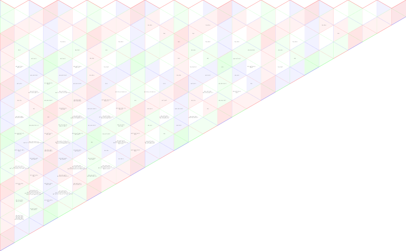
Figure 5: Triples for $p=3$

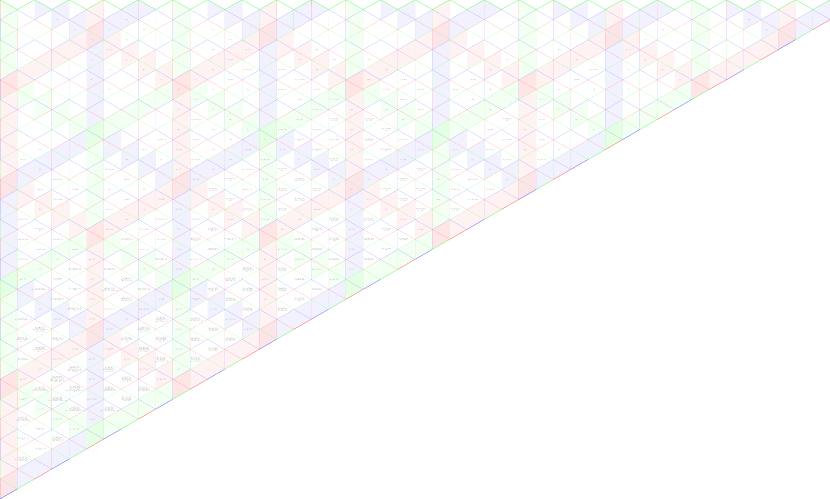
Figure 6: Triples for $p=5$

Figure 7: Triples for $p=7$

Figure 8: Triples for $p=11$

References

• [AMRW19] Pramod N. Achar, Shotaro Makisumi, Simon Riche and Geordie Williamson β€œKoszul duality for Kac-Moody groups and characters of tilting modules” In J. Amer. Math. Soc. 32.1, 2019, pp. 261–310 DOI: 10.1090/jams/905
• [BR20] Roman Bezrukavnikov and Simon Riche β€œHecke action on the principal block”, 2020 eprint: arXiv:2009.10587
• [BCP97] Wieb Bosma, John Cannon and Catherine Playoust β€œThe Magma algebra system. I. The user language” Computational algebra and number theory (London, 1993) In J. Symbolic Comput. 24.3-4, 1997, pp. 235–265 DOI: 10.1006/jsco.1996.0125
• [Jen18] Lars Thorge Jensen β€œp-Kazhdan-Lusztig Theory”, 2018 eprint: https://pure.mpg.de/rest/items/item_3117989_1/component/file_3117990/ content
• [Jen20] Lars Thorge Jensen β€œThe ABC of p-cells” In Selecta Math. (N.S.) 26.2, 2020, pp. Paper No. 28, 46 DOI: 10.1007/s00029-020-0552-1
• [LW18] George Lusztig and Geordie Williamson β€œBilliards and tilting characters for $\rm SL_{3}$” In SIGMA Symmetry Integrability Geom. Methods Appl. 14, 2018, pp. Paper No. 015, 22 DOI: 10.3842/SIGMA.2018.015
• [RW18] Simon Riche and Geordie Williamson β€œTilting modules and the $p$-canonical basis” In AstΓ©risque, 2018, pp. ix+184
• [RW20] Simon Riche and Geordie Williamson β€œSmith-Treumann theory and the linkage principle”, 2020 eprint: arXiv:2003.08522
Γ‰cole polytechnique fΓ©dΓ©rale de Lausanne, Route Cantonale, CH-1015 Lausanne, Switzerland