Distribution-free calibration guarantees for
histogram binning without sample splitting

Abstract

We prove calibration guarantees for the popular histogram binning (also called uniform-mass binning) method of Zadrozny and Elkan (2001). Histogram binning has displayed strong practical performance, but theoretical guarantees have only been shown for sample split versions that avoid ‘double dipping’ the data. We demonstrate that the statistical cost of sample splitting is practically significant on a credit default dataset. We then prove calibration guarantees for the original method that double dips the data, using a certain Markov property of order statistics. Based on our results, we make practical recommendations for choosing the number of bins in histogram binning. In our illustrative simulations, we propose a new tool for assessing calibration—validity plots—which provide more information than an ECE estimate. Code for this work will be made publicly available at https://github.com/aigen/df-posthoc-calibration.

1 Introduction

In classification, the goal is to learn a model that uses observed feature measurements to make a class prediction on the categorical outcome. However, for safety-critical areas such as medicine and finance, a single class prediction might be insufficient and reliable measures of confidence or certainty may be desired. Such uncertainty quantification is often provided by predictors that produce not just a class label, but a probability distribution over the labels. If the predicted probability distribution is consistent with observed empirical frequencies of labels, the predictor is said to be calibrated (Dawid, 1982).

In this paper we study the problem of calibration for binary classification; let $\mathcal{X}$ and $\smash{\mathcal{Y}=\{0,1\}}$ denote the feature and label spaces. We focus on the recalibration or post-hoc calibration setting, a standard statistical setting where the goal is to recalibrate existing (‘pre-learnt’) classifiers that are powerful and (statistically) efficient for classification accuracy, but do not satisfy calibration properties out-of-the-box. This setup is popular for recalibrating pre-trained deep nets. For example, Guo et al. (2017, Figure 4) demonstrated that a pre-learnt ResNet is initially miscalibrated, but can be effectively post-hoc calibrated. In the case of binary classification, the pre-learnt model can be an arbitrary predictor function that provides a classification ‘score’ $g\in\mathcal{G}$, where $\mathcal{G}$ is the space of all measurable functions from $\mathcal{X}\to[0,1]$. Along with $g$, we are given access to a calibration dataset of size $n\in\mathbb{N}$, $\mathcal{D}_{n}=\{(X_{i},Y_{i})\}_{i\in[n]}$, drawn independently from a distribution $P\equiv P_{X}\times P_{Y|X}$. The goal is to define a calibrator $\smash{H:\mathcal{G}\times(\mathcal{X}\times[0,1])^{n}\to\mathcal{G}}$, that ‘recalibrates’ $g$ to an approximately calibrated predictor $H(g,\mathcal{D}_{n})$ (formally defined shortly). We denote $H(g,\mathcal{D}_{n})$ as $h$. All probabilities in this paper are conditional on $g$ and thus conditional on the data on which $g$ is learnt.

Let $\mathbb{E}\left[\cdot\right]$ denote the expectation operator associated with $P$, interpreted marginally or conditionally depending on the context. The predictor $h$ is said to be perfectly calibrated if $\smash{\mathbb{E}\left[Y\mid h(X)\right]=h(X)}$ (almost surely). While perfect calibration is impossible in finite samples, we desire a framework to make transparent claims about how close $h$ is to being perfectly calibrated. The following notion proposed by Gupta et al. (2020) defines a calibrator that provides probably approximate calibration for chosen levels of approximation $\varepsilon\in(0,1)$ and failure $\alpha\in(0,1)$. For brevity, we skip the qualification ‘probably approximate’.

Definition 1 (Marginal calibration).

A calibrator $H:(g,\mathcal{D}_{n})\mapsto h$ is said to be $(\varepsilon,\alpha)$-marginally calibrated if for every predictor $g\in\mathcal{G}$ and distribution $P$ over $\mathcal{X}\times[0,1]$,

$${\text{Pr}}(\left\lvert\mathbb{E}\left[Y|h(X)\right]-h(X)\right\rvert\leq\varepsilon)\geq 1-\alpha.$$ (1)

The above probability is taken over both $X$ and $\mathcal{D}_{n}$ since $\smash{h=H(g,\mathcal{D}_{n})}$ contains the randomness of $\mathcal{D}_{n}$. The qualification marginal signifies that the inequality $\left\lvert\mathbb{E}\left[Y\mid h(X)\right]-h(X)\right\rvert\leq\varepsilon$ may not hold conditioned on $X$ or $h(X)$, but holds only on average. We now define a more stringent conditional notion of calibration, which requires that approximate calibration hold simultaneously (or conditionally) for every value of the prediction.

Definition 2 (Conditional calibration).

A calibrator $H:(g,\mathcal{D}_{n})\mapsto h$ is $(\varepsilon,\alpha)$-conditionally calibrated if for every predictor $g\in\mathcal{G}$ and distribution $P$ over $\mathcal{X}\times[0,1]$,

$${\text{Pr}}(\forall r\in\text{Range}(h),\left\lvert\mathbb{E}\left[Y\mid h(X)=r\right]-r\right\rvert\leq\varepsilon)\geq 1-\alpha.$$ (2)

In contrast to (1), the $\Pr$ above is only over $\mathcal{D}_{n}$. Evidently, if $H$ is conditionally calibrated, it is also marginally calibrated. The conditional calibration property (2) has a PAC-style interpretation: with probability $1-\alpha$ over $\mathcal{D}_{n}$, $h$ satisfies the following deterministic property:

$$\forall r\in\text{Range}(h),\left\lvert\mathbb{E}\left[Y\mid h(X)=r\right]-r\right\rvert\leq\varepsilon.$$ (3)

Marginal calibration does not have such an interpretation; we cannot infer from (1) a statement of the form “with probability $1-\gamma$ over $\mathcal{D}_{n}$, $h$ satisfies $\cdots$ ”.

Marginal and conditional calibration assess the truth of the event $\mathbbm{1}\left\{\left\lvert\mathbb{E}\left[Y\mid h(X)\right]-h(X)\right\rvert\leq\varepsilon\right\}$ for a given $\varepsilon$. Instead we can consider bounding the expected value of $\left\lvert\mathbb{E}\left[Y\mid h(X)\right]-h(X)\right\rvert$ for $X\sim P_{X}$. This quantity is known as the expected calibration error.

Definition 3 (Expected Calibration Error (ECE)).

For $p\in[1,\infty)$, the $\ell_{p}$-ECE of a predictor $h$ is

$$\ell_{p}\text{-ECE}(h)=\left(\mathbb{E}_{X}{\left\lvert\mathbb{E}\left[Y\mid h(X)\right]-h(X)\right\rvert^{p}}\right)^{1/p}.$$ (4)

Note that the expectation above is only over $X\sim P_{X}$ and not over $\mathcal{D}_{n}$. We can ask for bounds on the ECE of $h=H(g,\mathcal{D}_{n})$ that hold with high-probability or in-expectation over the randomness in $\mathcal{D}_{n}$. The conditional calibration property (3) for $h$ implies a bound on the $\ell_{p}$-ECE for every $p$, as formalized by the following proposition which also relates $\ell_{p}$-ECE for different $p$.

Proposition 1.

For any predictor $h$ and $1\leq p\leq q<\infty$,

$$\ell_{p}\text{-ECE}(h)\leq\ell_{q}\text{-ECE}(h).$$ (5)

Further, if (3) holds, then $\ell_{p}\text{-ECE}(h)\leq\varepsilon,\forall p\in[1,\infty)$.

The proof (in Appendix A) is a straightforward application of Hölder’s inequality. Informally, one can interpret the L.H.S. of (3) as the $\ell_{\infty}\text{-ECE}$ of $h$ so that (5) holds for $1\leq p\leq q\leq\infty$. Thus conditional calibration is the strictest calibration property we consider: if $H$ is $(\varepsilon,\alpha)$-conditionally calibrated, then (a) $H$ is $(\varepsilon,\alpha)$-marginally calibration and (b) with probability $1-\alpha$, $\ell_{p}\text{-ECE}(h)\leq\varepsilon$.

Example 1.

We verify Proposition 1 on a simple example, which also helps build intuition for the various notions of calibration. Suppose $h$ takes just two values: ${\text{Pr}}(h(X)=0.2)=0.9$ and ${\text{Pr}}(h(X)=0.8)=0.1$. Let $\mathbb{E}\left[Y\mid h(X)=0.2\right]=0.3$ and $\mathbb{E}\left[Y\mid h(X)=0.8\right]=0.6$. Then $\ell_{1}$-ECE$(h)=0.11<\ell_{2}$-ECE$(h)\approx 0.114$. Marginal calibration (1) for $H(\cdot,\cdot)\equiv h$ is satisfied for $(\varepsilon\geq 0.1,\alpha\leq 0.9)$, while the conditional calibration requirement (3) is only satisfied for $\varepsilon\geq 0.2$.

In this paper, we show that the histogram binning method of Zadrozny and Elkan (2001), described shortly, is calibrated in each of the above senses (marginal and conditional calibration; high-probability and in-expectation bounds on ECE), if the number of bins is chosen appropriately.

Some safety-critical domains may require calibration methods that are robust to the data-generating distribution. We refer to Definitions 1 and 2 as distribution-free (DF) guarantees since they are required to hold for all distributions over $(X,Y)$ without restriction. This paper is in the DF setting: the only assumption we make is that the calibration data $\mathcal{D}_{n}$ and $(X,Y)$ are independent and identically distributed (i.i.d.). Gupta et al. (2020, Theorem 3) showed that if $H$ is DF marginally calibrated with a meaningful value of $\varepsilon$ (formally, $\varepsilon$ can be driven to zero as sample size grows to infinity), then $H$ must necessarily produce only discretized predictions (formally, $\text{Range}(h)$ must be at most countable). We refer to such $H$ as ‘binning methods’ — this emphasizes that $H$ essentially partitions the sample-space into a discrete number of ‘bins’ and provides one prediction per bin (see Proposition 1 (Gupta et al., 2020)). Since our goal is DF calibration, we focus on binning methods.

1.1 Prior work on binning

Binning was initially introduced in the calibration literature for assessing calibration. Given a continuous scoring function $h$, if we wish to plot a reliability diagram (Sanders, 1963; Niculescu-Mizil and Caruana, 2005) or compute an ECE estimate (Miller, 1962; Sanders, 1963; Naeini et al., 2015), then $h$ must first be discretized using binning. A common binning scheme used for this purpose is ‘fixed-width binning’, where $[0,1]$ is partitioned into $B\in\mathbb{N}$ intervals (called bins) of width $1/B$ each and a single prediction is assumed for every bin. For example, if $B=10$, then the width of each bin is $0.1$, and if (say) $h(x)\in[0.6,0.7)$ then the prediction is assumed to be $0.65$.

Gupta et al. (2020, Theorem 3) showed that some kind of binning is in fact necessary to achieve DF calibration. The first binning method for calibration was proposed by Zadrozny and Elkan (2001) to calibrate a naive Bayes classifier. Their procedure is as follows. First, the interval $[0,1]$ is partitioned into $\smash{B\in\mathbb{N}}$ bins using the histogram of the $g(X_{i})$ values, to ensure that each bin has the same number of calibration points (plus/minus one). Thus the bins have nearly ‘uniform (probability) mass’. Then, the calibration points are assigned to bins depending on the interval to which the score $g(X_{i})$ belongs to, and the probability that $\smash{Y=1}$ is estimated for each bin as the average of the observed $Y_{i}$-values in that bin. This average estimates the ‘bias’ of the bin. The binning scheme and the bias estimates together define $h$. A slightly modified version of this procedure is formally described in Algorithm 1.

While Algorithm 1 was originally called histogram binning, it has also been referred to as uniform-mass binning in some works. In the rest of this paper, we use the latter terminology. Specifically, we refer to it as UMD, short for Uniform-Mass-Double-dipping. This stresses that the same data is used twice, both to determine inter-bin boundaries and to calculate intra-bin biases. UMD continues to remain a competitive benchmark in empirical work (Guo et al., 2017; Naeini et al., 2015; Roelofs et al., 2020), but no finite-sample calibration guarantees have been shown for it. Some asymptotic consistency results for a histogram regression algorithm closely related to UMD were shown by Parthasarathy and Bhattacharya (1961) (see also the work by Lugosi and Nobel (1996)). Zadrozny and Elkan (2002) proposed another popular binning method based on isotonic regression, for which some non-DF analyses exist (see Dai et al. (2020) and references therein). Recently, two recalibration methods closely related to UMD have been proposed, along with some theoretical guarantees that rely on sample-splitting — scaling-binning (Kumar et al., 2019) and sample split uniform-mass binning (Gupta et al., 2020).

In the scaling-binning method, the binning is performed on the output of another continuous recalibration method (such as Platt scaling (Platt, 1999)), and the bias for each bin is computed as the average of the output of the scaling procedure in that bin. This is unlike other binning methods, where the bias of each bin is computed as the average of the true outputs $Y_{i}$ in that bin. Kumar et al. (2019, Theorem 4.1) showed that under some assumptions on the scaling class (which includes injectivity), the ECE of the sample split scaling-binning procedure is $\varepsilon$-close to $\sqrt{2}\ \ell_{2}$-ECE of the scaling procedure if, roughly, $n=\Omega(\log B/\varepsilon^{2})$. However, the results of Gupta et al. (2020, Section 3.3) imply that there exist data distributions on which any injective scaling procedure itself has trivial ECE.

In sample split uniform-mass binning, the first split of the data is used to define the bin boundaries so that the bins are balanced. The second split of the data is used for estimating the bin biases, using the average of the $Y_{i}$-values in the bin. We refer to this version as UMS, for Uniform-Mass-Sample-splitting. Gupta et al. (2020, Theorem 5) showed that UMS is $(\varepsilon,\alpha)$-marginally calibrated if (roughly) $n=\Omega(B\log(B/\alpha)/\varepsilon^{2})$. To the best of our knowledge, this is the only known DF guarantee for a calibration method. However, in Section 2 we demonstrate that the constants in this guarantee are quite conservative, and the loss in performance due to sample splitting is practically significant on a real dataset.

1.2 Our contribution

We show tight DF calibration guarantees for the original method proposed by Zadrozny and Elkan (2001), UMD. While the existing theoretical analyses rely on sample splitting (Kumar et al., 2019; Gupta et al., 2020), it has been observed in experiments that double dipping to perform both bin formation and bias estimation on the same data leads to excellent practical performance (Zadrozny and Elkan, 2001; Guo et al., 2017; Kumar et al., 2019; Roelofs et al., 2020). Our work fills this gap in theory and practice.

We exploit a certain Markov property of order statistics, which are a set of classical, elegant results that are not well known outside of certain subfields of statistics (for one exposition of the Markov property, see Arnold et al. (2008, Chapter 2.4)). The strength of these probabilistic results is not widely appreciated — judging by their non-appearance in the ML literature — nor have they had implications for any modern AI applications that we are aware of. Thus, we consider it a central contribution of this work to have recognized that these mathematical tools can be brought to bear in order to shed light on a contemporary ML algorithm.

A simplified version of the Markov property is as follows: for order statistics $Z_{(1)},Z_{(2)},\ldots,Z_{(n)}$ of samples $\{Z_{i}\}_{i\in[n]}$ drawn i.i.d from any absolutely continuous distribution $Q$, and any indices $\smash{1<i<j\leq n}$, we have that

$$Z_{(j)}\perp Z_{(i-1)},Z_{(i-2)},\ldots,Z_{(1)}\mid Z_{(i)}.$$

For example, given the empirical median $M$, the points to its left are conditionally independent of the points to its right. Further each of these have a distribution that is identical to that of i.i.d. draws from $Z\sim Q$ when restricted to $Z<M$ (or $Z>M$). The implication is that if we form bins using the order statistics of the scores as the bin boundaries, then (a) the points within any bin are independent of the points outside that bin, and (b) conditioned on being in a given bin, say $B_{i}$, the points in the bin are i.i.d. with distribution $Q_{Z\mid Z\in B_{i}}$. When we split a calibration sample $\mathcal{D}$ and use one part $\mathcal{D}_{1}$ for binning and the other $\mathcal{D}\setminus\mathcal{D}_{1}$ for estimating bin probabilities, the points in $\mathcal{D}\setminus\mathcal{D}_{1}$ that belong to $B_{i}$ are also conditionally i.i.d. with distribution $Q_{Z\mid Z\in B_{i}}$, which is exactly what we accomplished without sample splitting. In short, the Markov property allows us to ‘double dip’ the data, i.e., use the same data for binning and estimating within-bin probabilities.

Organization. Section 2 motivates our research problem by showing that UMS is sample-inefficient both in theory and practice. Empirical evidence is provided through a novel diagnostic tool called validity plots (Section 2.1). Section 3 presents UMD formally along with its analysis (main results in Theorems 3 and 4). Section 4 contains illustrative simulations. Proofs are in the supplement.

2 Sample split uniform-mass binning is inefficient

The DF framework encourages development of algorithms that are robust to arbitrarily distributed data. At the same time, the hope is that the DF guarantees are adaptive to real data and give meaningful bounds in practice. In this section, we assess if the practical performance of uniform-mass-sample-splitting (UMS) is well explained by its DF calibration guarantee (Gupta et al., 2020). As far as we know, this is the only known DF guarantee for a calibration method. However, we demonstrate that the guarantee is quite conservative. Further, we demonstrate that sample splitting leads to a drop in performance on a real dataset.

Suppose we wish to guarantee $\smash{(\varepsilon,\alpha)=(0.1,0.1)}$-marginal calibration with $B=10$ bins using UMS. We unpacked the DF calibration bound for UMS, and computed that to guarantee $\smash{(0.1,0.1)}$-marginal calibration with $10$ bins, roughly $n\geq 17500$ is required. The detailed calculations can be found in Appendix B. This sample complexity seems conservative for a binary classification problem. In Section 2.2, we use an illustrative experiment to show that the $n$ required to achieve the desired level of calibration is indeed much lower than $17500$. Our experiment uses a novel diagnostic tool called validity plots, introduced next.

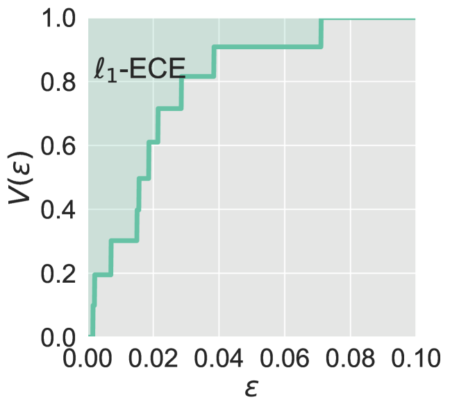
(a) An illustrative validity plot. We can read off that marginal calibration is achieved for $(\varepsilon,\alpha)=(0.04,0.1)$ and $(0.03,0.2)$. The $\ell_{1}$-ECE estimate is roughly $0.023$.

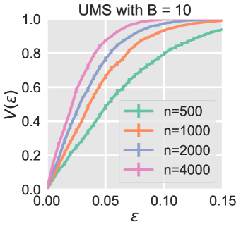
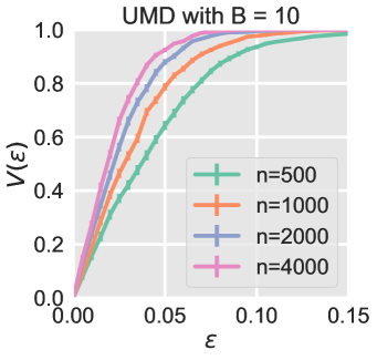
(b) Validity plots comparing UMD and UMS on the CREDIT dataset. The plots show that UMD has higher validity $V(\varepsilon)$ for the same values of $n,\varepsilon$, and thus lower $\ell_{1}$-ECE. For example, for $n=1000$ and $\varepsilon=0.05$, UMS has $V(\varepsilon)\approx 0.63$, while UMD has $V(\varepsilon)\approx 0.79$.

Figure 1: Validity plots display estimates of $\smash{V(\varepsilon)={\text{Pr}}(\left\lvert\mathbb{E}\left[Y\mid h(X)\right]-h(X)\right\rvert\leq\varepsilon)}$ as $\varepsilon$ varies. Validity plots are described in Section 2.1. The experimental setup for Figure 1(b) is presented in Section 2.2.

2.1 Validity plots

Validity plots assess the marginal calibration properties of a calibration method by displaying estimates of the LHS of (1) as $\varepsilon$ varies. Define the function $V:[0,1]\to[0,1]$ given by $V(\varepsilon)=\Pr(\left\lvert\mathbb{E}\left[Y\mid h(X)\right]-h(X)\right\rvert\leq\varepsilon)$. By definition of $V$, $H$ is $(\varepsilon,1-V(\varepsilon))$-marginally calibrated for every $\varepsilon$. For this reason, we call the graph of $V$, $\{(\varepsilon,V(\varepsilon)):\varepsilon\in[0,1]\}$, as the ‘validity curve’. (The term “curve” is used informally since $V$ may have jumps.) Note the following neat relationship between the $\ell_{1}\text{-ECE}$ and the area-under-the-curve (AUC) of the validity curve:

$$\mathbb{E}\left[\ell_{1}\text{-ECE}(h)\right] =\mathbb{E}\left[\left\lvert\mathbb{E}\left[Y\mid h(X)\right]-h(X)\right\rvert\right]$$

$$= \int_{0}^{1}{\text{Pr}}(\left\lvert\mathbb{E}\left[Y\mid h(X)\right]-h(X)\right\rvert>\varepsilon)\ d\varepsilon$$

$$= 1-\int_{0}^{1}{\text{Pr}}(\left\lvert\mathbb{E}\left[Y\mid h(X)\right]-h(X)\right\rvert\leq\varepsilon)\ d\varepsilon$$

$$= 1-\int_{0}^{1}V(\varepsilon)\ d\varepsilon=1-\text{AUC(validity curve)}.$$

A validity plot is a finite sample estimate of the validity curve on a single calibration set $\mathcal{D}_{n}$ and test set $\mathcal{D}_{\text{test}}$. We now outline the steps for constructing a validity plot. First, $h$ is learned using $\mathcal{D}_{n}$ and $g$. Next, if $h$ is not a binning method, it must be discretized through binning in order to enable estimation of $\mathbb{E}\left[Y\mid h(X)\right]$. This is identical to the binning step required by plugin ECE estimators and reliability diagrams. For example, one can use fixed-width binning as described in the first paragraph of Section 1.1. In this paper, we empirically assess only binning methods, and so an additional binning step is not necessary. Next, the empirical distribution on $\mathcal{D}_{\text{test}}$ is used as a proxy for the true distribution of $(X,Y)$, to estimate $V(\varepsilon)$:

$$\widehat{V}(\varepsilon)=\frac{\sum_{(X_{i},Y_{i})\in\mathcal{D}_{\text{test}}}\mathbbm{1}\left\{\left\lvert\mathbb{E}_{\widehat{P}}\left[Y\mid h(X)=h(X_{i})\right]-h(X_{i})\right\rvert\leq\varepsilon\right\}}{\left\lvert\mathcal{D}_{\text{test}}\right\rvert},\text{ where}$$

$$\quad\mathbb{E}_{\widehat{P}}\left[Y\mid h(X)=h(x)\right]\equiv\frac{\sum_{(X_{i},Y_{i})\in\mathcal{D}_{\text{test}}}Y_{i}{\mathbbm{1}\left\{h(X_{i})=h(x)\right\}}}{\sum_{(X_{i},Y_{i})\in\mathcal{D}_{\text{test}}}\mathbbm{1}\left\{h(X_{i})=h(x)\right\}}.$$ (6)

For different values of $\varepsilon\in[0,1]$ on the X-axis, the estimate of $V(\varepsilon)$ is plotted on the Y-axis to form the validity plot. Like the AUC of a validity curve corresponds to $\mathbb{E}\left[\ell_{1}\text{-ECE}\right]$, the AUC of a validity plot corresponds to the plugin $\ell_{1}$-ECE estimate (Naeini et al., 2015). (There may be small differences in practice since we draw the validity plot for a finite grid of values in $[0,1]$.) Thus validity plots convey the $\ell_{1}$-ECE estimate and more.

Figure 1(a) displays an illustrative validity plot for a binning method with $B=10$. $V$ is a right-continuous step function with at most $\left\lvert\text{Range}(h)\right\rvert\leq B$ many discontinuities. Each $\varepsilon$ for which there is a discontinuity in $V$ corresponds to a bin that has $\left\lvert\mathbb{E}\left[Y\mid h(X)=r\right]-r\right\rvert=\varepsilon$, and the incremental jump in the value of $V$, $V(\varepsilon)-V(\varepsilon^{-})$, corresponds to the fraction of test points in that bin. Figure 1(a) was created using UMD, and thus each jump corresponds to roughly a $1/B=0.1$ fraction of the test points. The $\varepsilon$ values for the bins are approximately $10^{-3}\cdot(1.5,2,8,16,17,19,22,29,39,71)$.

Unlike reliability diagrams (Niculescu-Mizil and Caruana, 2005), validity plots do not convey the predictions $h(X)$ to which the $\varepsilon$ values correspond to, or the direction of miscalibration (whether $h(X)$ is higher or lower than $\mathbb{E}\left[Y\mid h(X)\right]$). On the other hand, validity plots convey the bin frequencies for every bin without the need for a separate histogram (such as the top panel in Niculescu-Mizil and Caruana (2005, Figure 1)). In our view, validity plots also ‘collate’ the right entity; we can easily read off from a validity plot practically meaningful statements such as “for 90% of the test points, the miscalibration is at most $0.04$”.

We can create a smoother validity plot that better estimates $V$ by using multiple runs based on subsampled or bootstrapped data. To do this, for every $\varepsilon\in[0,1]$, $\widehat{V}(\varepsilon)$ is computed separately for each run and the mean value is plotted as the estimate of $V(\varepsilon)$. In our simulations, we always perform multiple runs, and also show $\pm$std-dev-of-mean in the plot. Figure 1(b) displays such validity plots (further details presented in the following subsection).

It is well known that plugin ECE estimators for a binned method are biased towards slightly overestimating the ECE (e.g., see Bröcker (2012); Kumar et al. (2019); Widmann et al. (2019)). For the same reasons, $\widehat{V}(\varepsilon)$ is a biased underestimate of $V(\varepsilon)$. In other words, the validity plot is on average below the true validity curve. The reason for this bias is that to estimate ECE as well as to create validity plots, we compute $\left\lvert\mathbb{E}_{\widehat{P}}\left[Y\mid h(X)\right]-h(X)\right\rvert$ which can be written as $\left\lvert\mathbb{E}\left[Y\mid h(X)\right]+\text{mean-zero-noise}-h(X)\right\rvert$. On average, the noise term will lead to overestimating $\left\lvert\mathbb{E}\left[Y\mid h(X)\right]-h(X)\right\rvert$. However, the noise term is small if there is enough test data (if $n_{b}$ is the number of test points in bin $b$, then the noise term is $O(\sqrt{1/n_{b}})$ w.h.p.). Further, it is highly unlikely that the noise will help some methods and hurts others. Thus validity plots can be reliably used to make inferences on the relative performance of different calibration methods. While there exist unbiased estimators for $(\ell_{2}\text{-ECE})^{2}$ (Bröcker, 2012; Widmann et al., 2019), we are not aware of any unbiased $\ell_{1}$-ECE estimators. If such an estimator is proposed in the future, the same technique will also improve validity plots.

2.2 Comparing UMS and UMD using validity plots

Figure 1(b) uses validity plots to assess UMS and UMD on CREDIT, a UCI credit default dataset. The task is to accurately predict the probability of default. The experimental protocol is as follows. The entire feature matrix is first normalized. CREDIT has 30K (30,000) samples which are randomly split (once for the entire experiment) into splits (A, B, C) = (10K, 5K, 15K). First, $g$ is formed by training a logistic regression model on split A and then re-scaling the learnt model using Platt scaling on split B (Platt scaling before binning was suggested by Kumar et al. (2019); we also observed that this helps in practice). Next, the calibration set $\mathcal{D}_{n}$ is formed by randomly subsampling $n$ ($\leq$10K) points from split C (without replacement). From the remaining points in split C, a test set of size 5K is subsampled (without replacement). The entire subsampling from split C is repeated 100 times to create 100 different calibration and test sets. For a given subsample, UMS/UMD with $B=10$ is trained on the calibration set (with 50:50 sample splitting for UMS), and $\widehat{V}(\varepsilon)$ for every $\varepsilon$ is estimated on the test set. Finally, the (mean$\pm$std-dev-of-mean) of $\widehat{V}(\varepsilon)$ is plotted with respect to $\varepsilon$. This experimental setup assesses marginal calibration for a fixed $g$, in keeping with our post-hoc calibration setting.

The validity plot in Figure 1(b) (left) indicates that the desired $(0.1,0.1)$-marginal calibration is achieved by UMS with just $\smash{n=1000}$. Contrast this to $\smash{n\geq 17500}$ required by the theoretical bound, as computed in Appendix B. In fact, $\smash{n=4000}$ nearly achieves $(0.05,0.1)$-marginal calibration. This gap occurs because the analysis of UMS is complex, with constants stacking up at each step.

Next, consider the validity plot for UMD in Figure 1(b) (right). By avoiding sample splitting, UMD achieves $(0.1,0.1)$-marginal calibration at $\smash{n=500}$. In Section 3 we show that $n\geq 1500$ is provably sufficient for $(0.1,0.1)$-marginal calibration and $n\geq 2900$ is sufficient for $(0.1,0.1)$-conditional calibration. Some gap in theory and practice is expected since the theoretical bound is DF, and thus applies no matter how anomalous the data distribution is. However, the gap is much smaller compared to UMS, due to a clean analysis. In Section 4, we illustrate that the gap nearly vanishes for larger $n$. Section 4 also introduces the related concept of conditional validity plots that assess conditional calibration.

3 Distribution-free analysis of uniform-mass binning without sample splitting

Define the random variables $S=g(X)$; $S_{i}=g(X_{i})$ for $\smash{i\in[n]}$, called scores. Let $\smash{(S,Y)\sim Q}$ and $\smash{S\sim Q_{S}}$. In binning, we wish to use the calibration data $\smash{\{(S_{i},Y_{i})\}_{i\in[n]}\sim Q^{n}}$ to (a) define a binning function $\mathcal{B}:[0,1]\to[B]$ for some number of bins $B\in\mathbb{N}$, and (b) estimate the biases in the bins $\smash{\{\Pi_{b}:=\mathbb{E}\left[Y\mid\mathcal{B}(S)=b\right]\}_{b\in[B]}}$. We denote the bias estimates as $\widehat{\Pi}_{b}$. The approximately calibrated function is then defined as $h(\cdot)=\widehat{\Pi}_{\mathcal{B}(\cdot)}$.

Suppose the number of recalibration points is $\smash{n\approx 150}$. In the absence of known properties of the data (i.e., in the DF setting), it seems reasonable to have $\smash{B=1}$ and define $H(g,\mathcal{D}_{n})$ as the constant function $h(\cdot):=n^{-1}\sum_{i=1}^{n}Y_{i}.$ Formally, $\smash{n=150}$ leads to the following Hoeffding-based confidence interval: with probability at least $0.9$, $\left\lvert n^{-1}\sum_{i=1}^{n}Y_{i}-\mathbb{E}Y\right\rvert\leq\sqrt{\log(2/0.1)/(2\cdot 150)}\approx 0.1$. In other words, if $\smash{n=150}$, $H$ satisfies $(0.1,0.1)$-marginal calibration. Of course, having a single bin completely destroys sharpness of $h$, but it’s an instructive special case.

Suppose now that $n\approx 300$, and we wish to learn a non-constant $h$ using two bins. If $g$ is informative, we hope that $\mathbb{E}\left[Y\mid g(X)=\cdot\right]$ is roughly a monotonically increasing function. In light of this belief, it seems reasonable to choose a threshold $t$ and identify the two bins as: $\smash{g(X)\leq t}$ and $\smash{g(X)>t}$. A natural choice for $t$ is $M=\text{Median}(S_{1},\ldots,S_{n})$ since this ensures that both bins get the same number of points (plus/minus one). This is the motivation for UMD. In this case, $h$ and $\widehat{\Pi}$ are defined as,

$$h(\cdot):=\left\{\begin{array}[]{ll}\widehat{\Pi}_{1}:=\text{Average}(\smash{Y_{i}:S_{i}\leq M})\mbox{ if }g(\cdot)\leq M\\ \widehat{\Pi}_{2}:=\text{Average}(\smash{Y_{i}:S_{i}>M})\mbox{ if }g(\cdot)>M.\end{array}\right.$$ (7)

Suppose $M$ were the true median of $Q_{S}$ instead of the empirical median. Then $h$ has a calibration guarantee obtained by applying a Bernoulli concentration inequality separately for both bins and using a union bound (this is done formally by Gupta et al. (2020, Theorem 4)). In UMS, we try to emulate the true median case by using one split of the data to estimate the median. $\widehat{\Pi}$ is then computed on the second (independent) split of the data, and concentration inequalities can be used to provide calibration guarantees.

UMD does not sample split: in equation (7) above, $M$ is computed using the same data that is later used to estimate $\widehat{\Pi}$. On the face of it, this double dipping eliminates the independence of the $Y_{i}$ values required to apply a concentration inequality. However, we show that the independence structure can be retained if UMD is slightly modified. This subtle modification is to remove a single point from the bias estimation, namely the $Y_{i}$ corresponding to the median $M$. (In comparison, in UMS we typically remove a fixed ratio of $n$.) The informal argument is as follows.

For simplicity, suppose $Q_{S}$ is absolutely continuous (with respect to the Lebesgue measure), so that the $S_{i}$’s are almost surely distinct, and suppose that the number of samples is odd: $n=2m+1$. Denote the ordered scores as $\smash{S_{(1)}<S_{(2)}<\ldots<S_{(n)}}$ and let $Y_{(i)}$ denote the label corresponding to the score $S_{(i)}$. Thus $\smash{\widehat{\Pi}_{1}=m^{-1}\sum_{i=1}^{m}Y_{(i)}}$ and $M=S_{(m+1)}$. Clearly, $(S_{(i)},Y_{(i)})$ is not independent of $S_{(m+1)}$ for any $i$. However, it turns out that the following property is true: conditioned on $S_{(m+1)}$, the unordered values $\{(S_{(i)},Y_{(i)})\}_{i\in[m]}$ can be viewed as $m$ independent samples identically distributed as $\smash{(S,Y)}$, given $S<S_{(m+1)}$. (Note that $(S,Y)$ is an unseen and independent random variable.) Thus, we can use Hoeffding’s inequality to assert: ${\text{Pr}}(|\mathbb{E}\left[Y\mid M,S<M\right]-\widehat{\Pi}_{1}|\geq\varepsilon\mid M,S<M)\leq 2\exp\left(-2m\varepsilon^{2}\right).$ This can be converted to a calibration guarantee on the first bin. The same bound can be shown if $S>M$, for the estimate $\widehat{\Pi}_{2}=m^{-1}\sum_{i=m+1}^{2m+1}Y_{(i)}$. Using a union bound gives a calibration guarantee that holds for both bins simultaneously, which in turn gives conditional calibration.

In the following subsection, we show some key lemmas regarding the order statistics of the $S_{i}$’s. These lemmas formalize what was argued above: careful double dipping does not eliminate the independence structure. In Section 3.2, we formalize the modified UMD algorithm, and prove that it is DF calibrated. Based on the guarantee for the modified version, Corollary 1 finally shows that the original UMD itself is DF calibrated.

Simplifying assumption. In the following analysis, we assume that $g(X)$ is absolutely continuous with respect to the Lebesgue measure, and thus has a probability density function (pdf). This assumption is made at no loss of generality, for reasons discussed in Appendix C.1.

3.1 Key lemmas on order statistics

Consider two indices $i,j\in[n]$. The score $S_{i}$ is not independent of the order statistic $S_{(j)}$. However, it turns out that conditioned on $S_{(j)}$, the distribution of $S_{i}$ given $S_{i}<S_{(j)}$, is identical to the distribution of an unseen score $S$, given $S<S_{(j)}$. The following lemmas (both proved in Appendix A) state versions of this fact that are useful for our analysis of UMD.

We first set up some notation. $S$ is assumed to have a pdf, denoted as $f$. For some $\smash{1\leq l<u\leq n}$, consider the set of indices $\smash{\{i:S_{(l)}<S_{i}<S_{(u)}\}}$, and index them arbitrarily as $\{t_{1},t_{2},\ldots,t_{u-l-1}\}$. This is just an indexing and not an ordering; in particular it is not necessary that $S_{t_{1}}=S_{(l+1)}$. For $j\in\{l+1,\ldots,u-1\}$, define $S_{\{j\}}=S_{t_{j-l}}$. Thus the set $\{S_{\{j\}}:j\in\{l+1,\ldots,u-1\}\}$ corresponds to the unordered $S_{i}$ values between $S_{(l)}$ and $S_{(u)}$.

Lemma 1.

Fix $l,u\in[n]$ such that $l<u$. The conditional density of the unordered $S_{i}$ values between the order statistics $S_{(l)},S_{(u)}$, $f(S_{\{l+1\}},\ldots,S_{\{u-1\}}\mid S_{(l)},S_{(u)}),$ is identical to the density of independent $S^{\prime}_{i}\sim Q_{S}$, conditional on lying between $S_{(l)},S_{(u)}$:

$$f(S^{\prime}_{1},\ldots,S^{\prime}_{u-l-1}\mid S_{(l)},S_{(u)},S_{(l)}<\{S^{\prime}_{i}\}_{i\in[u-l-1]}<S_{(u)}).$$

In the final analysis, $S_{(l)}$ and $S_{(u)}$ will represent the scores at consecutive bin boundaries, which define the binning scheme. Lemma 2 is similar to Lemma 1, but with conditioning on all bin boundaries (order statistics) simultaneously. To state it concisely, define $S_{(0)}:=0$ and $S_{(n+1)}:=1$ as fixed hypothetical ‘order statistics’.

Lemma 2.

Fix any $\smash{B-1}$ indices $k_{1},k_{2},\ldots k_{B-1}$ such that $\smash{0=k_{0}<k_{1}<\ldots<k_{B-1}<k_{B}=n+1}$. For any $b\in[B]$, the conditional density of the unordered $S_{i}$ values between the order statistics $S_{(k_{b-1})},S_{(k_{b})}$, $f(S_{\{k_{b-1}+1\}},\ldots,S_{\{k_{b}-1\}}\mid S_{(k_{0})},\ldots,S_{(k_{B})})$, is identical to the conditional density

$$f(S^{\prime}_{1},\ldots,S^{\prime}_{k_{b}-k_{b-1}-1}\mid S_{(k_{0})},\ldots,S_{(k_{B})},$$

$$\qquad\text{for every $i\in[k_{b}-k_{b-1}-1]$, $S_{(k_{b-1})}<S^{\prime}_{i}<S_{(k_{b})}$}))$$

of independent random variables $S^{\prime}_{i}\sim Q_{S}$.

3.2 Main results

Algorithm 1 UMD: Uniform-mass binning without sample splitting

1:  Input: Scoring function $\smash{g:\mathcal{X}\to[0,1]}$, #bins $B$, calibration data $(X_{1},Y_{1}),(X_{2},Y_{2}),\ldots,(X_{n},Y_{n})$

2:  Output: Approximately calibrated function $h$

3:  $(S_{1},S_{2},\ldots,S_{n})\leftarrow(g(X_{1}),g(X_{2}),\ldots,g(X_{n}))$ 

4:  $\smash{(S_{(1)},S_{(2)},\ldots,S_{(n)})\leftarrow\text{order-stats}(S_{1},S_{2},\ldots,S_{n})}$ 

5:  $(Y_{(1)},Y_{(2)},\ldots,Y_{(n)})\leftarrow(Y_{1},Y_{2},\ldots,Y_{n})$ ordered as per the ordering of $(S_{(1)},S_{(2)},\ldots,S_{(n)})$ 

6:  $\Delta\leftarrow(n+1)/B$ 

7:  $\widehat{\Pi}\leftarrow$ empty array of size $B$ 

8:  $A\leftarrow 0\text{-indexed array}([0,\lceil\Delta\rceil,\lceil 2\Delta\rceil,\ldots,n+1])$ 

9:  for $b\leftarrow 1$ to $B$ do

10:     $l\leftarrow A_{b-1}$ 

11:     $u\leftarrow A_{b}$ 

12:     $\widehat{\Pi}_{b}\leftarrow$ Mean($Y_{(l+1)},Y_{(l+2)},\ldots,Y_{(u-1)}$) 

13:  end for

14:   $(S_{(0)},S_{(n+1)})\leftarrow(0,1)$ 

15:  $h(\cdot)\leftarrow\sum_{b=1}^{B}\mathbbm{1}\left\{S_{(A_{b-1})}\leq g(\cdot)<S_{(A_{b})}\right\}\widehat{\Pi}_{b}$ 

UMD is described in Algorithm 1 (in the description, $\lfloor\cdot\rfloor$ and $\lceil\cdot\rceil$ denote the floor and ceiling operators respectively). UMD takes input $(g,\mathcal{D}_{n})$ and outputs $h$. There is a small difference between UMD as stated and the proposal by Zadrozny and Elkan (2001). The original version also uses the calibration points that define the bin boundaries for bias estimation — this corresponds to replacing line 12 with

$$\text{line~{}\ref{line:removed-mean}: }\widehat{\Pi}_{b}\leftarrow\text{Mean}(Y_{(l+1)},\ldots,Y_{(u-1)},\bm{Y_{(u)}}),\text{for }b<B.$$

The two algorithms are virtually the same; after stating the calibration guarantee for UMD, we show the result for the original proposal as a corollary.

By construction, every bin defined by UMD has at least $\smash{\lfloor n/B\rfloor-1}$ many points for mean estimation. Thus, UMD effectively ‘uses’ only $B-1$ points for bin formulation using quantile estimation. We prove the following calibration guarantee for UMD in Appendix A.

Theorem 3.

Suppose $g(X)$ is absolutely continuous with respect to the Lebesgue measure and $n\geq 2B$. UMD is $(\varepsilon,\alpha)$-conditionally calibrated for any $\alpha\in(0,1)$ and

$$\varepsilon=\sqrt{\frac{\log(2B/\alpha)}{2(\lfloor n/B\rfloor-1)}}.$$ (8)

Further, for every distribution $P$, w.p. $1-\alpha$ over the calibration data $\mathcal{D}_{n}$, for all $p\in[1,\infty)$, $\ell_{p}\text{-ECE}(h)\leq\varepsilon$.

Note that since UMD is $(\varepsilon,\alpha)$-conditionally calibrated, it is also $(\varepsilon^{\prime},\alpha)$-conditionally calibrated for any $\varepsilon^{\prime}\in(\varepsilon,1)$. The absolute continuity requirement for $g(X)$ can be removed with a randomization trick discussed in Section C.1, to make the result fully DF. The proof sketch is as follows. Given the bin boundaries, the scores in each bin are independent, as shown by Lemma 2. We use this to conclude that the $Y_{i}$ values in each bin $b$ are independent and distributed as $\text{Bern}(\mathbb{E}\left[Y\mid\mathcal{B}(X)=b\right])$. The average of the $Y_{i}$ values thus concentrates around $\mathbb{E}\left[Y\mid\mathcal{B}(X)=b\right]$. Since each bin has at least $(\lfloor n/B\rfloor-1)$ points, Hoeffding’s inequality along with a union bound across bins gives conditional calibration for the value of $\varepsilon$ in (8).

The convenient property that every bin has at least $\lfloor n/B\rfloor-1$ calibration points for mean estimation is not satisfied deterministically even if we used the true quantiles of $g(X)$. In fact, as long as $B=o(n)$, the $\varepsilon$ in (8) approaches the $\varepsilon$ we would get if all the data was used for bias estimation, with at least $\lfloor n/B\rfloor$ points in each bin:

$$\text{if $B=o(n)$, }\lim_{n\to\infty}\left\lvert\sqrt{\frac{\log(2B/\alpha)}{2(\lfloor n/B\rfloor-1)}}-\sqrt{\frac{\log(2B/\alpha)}{2(\lfloor n/B\rfloor)}}\right\rvert=0.$$

In comparison to the clean proof sketch above, UMS requires a tedious multi-step analysis:

1. Suppose the sizes of the two splits are $n_{1}$ and $n_{2}$. Performing reliable quantile estimation on the first split of the data requires $n_{1}=\Omega(B\log(B/\alpha))$ (Kumar et al., 2019, Lemma 4.3)).

2. The estimated quantiles have the guarantee that the expected number of points falling into a bin, on the second split is $\geq n_{2}/2B$. A high probability bound is used to lower bound the actual number of points in each bin. This lower bound is $(n_{2}/2B)-\sqrt{n_{2}\log(2B/\alpha)/2}$ (Gupta et al., 2020, Theorem 5).

This multi-step analysis leads to a loose bound due to constants stacking up, as discussed in Section 2.

A guarantee for the original UMD procedure follows as an immediate corollary of Theorem 3. This is because the modification to line 12 can change every estimate $\widehat{\Pi}_{b}$ by at most $1/(\lfloor n/B\rfloor)$ due to the following fact regarding averages: for any $b\in\mathbb{N},a\in\{0,1,\ldots,b\}$,

$$\max\left(\left\lvert\frac{a}{b+1}-\frac{a}{b}\right\rvert,\left\lvert\frac{a+1}{b+1}-\frac{a}{b}\right\rvert\right)\leq\frac{1}{b+1}.$$ (9)

Using (9), we prove the following corollary in Appendix A.

Corollary 1.

Suppose $g(X)$ is absolutely continuous with respect to the Lebesgue measure and $n\geq 2B$. The original UMD algorithm (Zadrozny and Elkan, 2001) is $(\varepsilon,\alpha)$-conditionally calibrated for any $\alpha\in(0,1)$ and

$$\varepsilon=\sqrt{\frac{\log(2B/\alpha)}{2(\lfloor n/B\rfloor-1)}}+\frac{1}{\lfloor n/B\rfloor}.$$ (10)

Further, for every distribution $P$, w.p. $1-\alpha$ over the calibration data $\mathcal{D}_{n}$, for all $p\in[1,\infty)$, $\ell_{p}\text{-ECE}(h)\leq\varepsilon$.

As claimed in Section 2.2, if $(n,\alpha,B)=(2900,0.1,10)$, (10) gives $\smash{\varepsilon<0.1}$. The difference between (10) and (8) is small. For example, we computed that if $\smash{\varepsilon\leq 0.1}$, $\smash{\alpha\leq 0.5}$, $B\geq 5$, then (8) requires $n/B\geq 150$, and thus the additional term in (10) is at most 0.007. Likewise, in practice, we expect both versions to perform similarly.

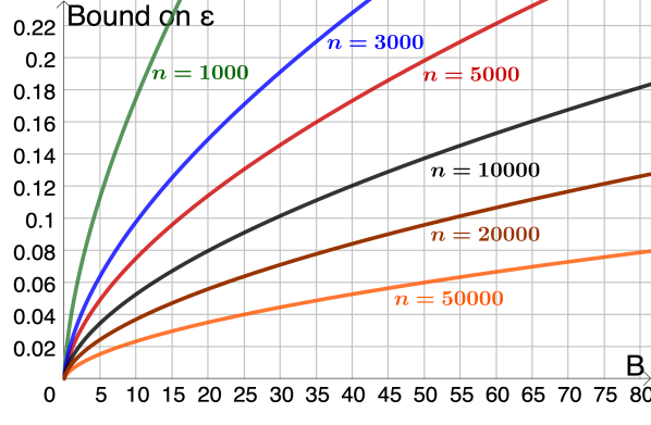
Figure 2: Plots displaying the relationship (8) between $\varepsilon$ and $B$ for $\alpha=0.1$ and different values of $n$. Some indicative suggestions based on the plot: if $n=1$K, choose $B=5$ (gives $\varepsilon\leq 0.12$); if $n=5$K, choose $B=10$ (gives $\varepsilon\leq 0.08$); if $n=20$K, choose $B=22$ (gives $\varepsilon\leq 0.06$).

At the end of the day, a practitioner may ask: “Given $n$ points for recalibration, how should I use Theorem 3 to decide $B$?” Smaller $B$ gives better bounds on $\varepsilon$, but larger $B$ implicitly means that the $h$ learnt is sharper. As $n$ becomes higher, one may like to have higher sharpness (higher $B$), but at the same time more precise calibration (lower $\varepsilon$ and thus lower $B$). We provide a (subjective) discussion on how to balance these two requirements.

First, we suggest fixing a rough domain-dependent probability of failure $\alpha$. Since the dependence of $\varepsilon$ on $\alpha$ in (8) is $\log(1/\alpha)$, small changes in $\alpha$ do not affect $\varepsilon$ too much. Typically, 10-20% failure rate is acceptable, so let us set $\alpha=0.1$. (For a highly sensitive domain, one can set $\alpha=0.01$.) Then, constraint (8) roughly translates to $\varepsilon=\sqrt{B\log(20B)/2n}$. For a fixed $n$, this is a relationship between $\varepsilon$ and $B$, that can be plotted as a curve with $B$ as the independent parameter and $\varepsilon$ as the dependent parameter. Finally, one can eyeball the curve to identify a $B$. We plot such curves in Figure 2 for a range of values of $n$. The caption shows examples of how one can choose $B$ to balance calibration (small $\varepsilon$) and sharpness (high $B$).

While $(\varepsilon,\alpha)$-conditional calibration implies $(\varepsilon,\alpha)$-marginal calibration, we expect to have marginal calibration with smaller $\varepsilon$. Such an improved guarantee can be shown if the bin biases $\widehat{\Pi}_{b}$ estimated by Algorithm 1 are distinct. In Appendix C, we propose a randomized version of UMD (Algorithm 2) which guarantees uniqueness of the bin biases. Algorithm 2 satisfies the following calibration guarantee (proved in Appendix A).

Theorem 4.

Suppose $n\geq 2B$ and let $\delta>0$ be an arbitrarily small randomization parameter. Algorithm 2 is $(\varepsilon_{1},\alpha)$-marginally and $(\varepsilon_{2},\alpha)$-conditionally calibrated for any $\alpha\in(0,1)$,

$$\varepsilon_{1}=\sqrt{\frac{\log(2/\alpha)}{2(\lfloor n/B\rfloor-1)}}+\delta\text{, }\varepsilon_{2}=\sqrt{\frac{\log(2B/\alpha)}{2(\lfloor n/B\rfloor-1)}}+\delta.$$ (11)

Further, for every distribution $P$, (a) w.p. $1-\alpha$ over the calibration data $\mathcal{D}_{n}$, for all $p\in[1,\infty)$, $\ell_{p}\text{-ECE}(h)\leq\varepsilon_{2}$, and (b) $\mathbb{E}_{\mathcal{D}_{n}}\left[\ell_{p}\text{-ECE}(h)\right]\leq\sqrt{B/2n}+\delta$ for all $p\in[1,2]$.

In the proof, we use the law of total expectation to avoid taking a union bound in the marginal calibration result; this gives a $\sqrt{\log(2/\alpha)}$ term in $\varepsilon_{1}$ instead of the $\sqrt{\log(2B/\alpha)}$ in $\varepsilon_{2}$. Theorem 4 also does not require absolute continuity of $g(X)$. As claimed in Section 2.2, if $(n,\alpha,B)=(1500,0.1,10)$, (11) gives $\smash{\varepsilon_{1}<0.1}$ (for small enough $\delta$).

(a) Marginal validity plots.

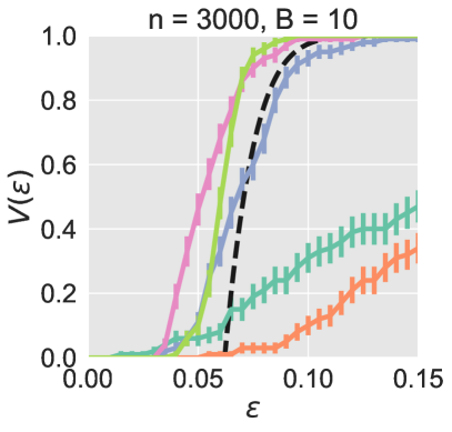
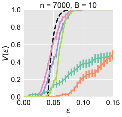
(b) Conditional validity plots.

Figure 3: UMD performs competitively on the CREDIT dataset. The guarantee of Theorem 4 closely matches empirical behavior.

4 Simulations

We perform illustrative simulations on the CREDIT dataset with two goals: (a) to compare the performance of UMD to other binning methods and (b) to show that the guarantees we have shown are reasonably tight, and thus, practically useful. In addition to validity plots, which assess marginal calibration, we use conditional validity plots, that assess conditional calibration. Let $\smash{V:[0,1]\to[0,1]}$ be given by $V(\varepsilon)={\text{Pr}}(\forall r\in\text{Range}(h),\left\lvert\mathbb{E}\left[Y\mid h(X)=r\right]-r\right\rvert\leq\varepsilon)$. Given a test set $\mathcal{D}_{\text{test}}$, we first compute $\mathbb{E}_{\widehat{P}}\left[Y\mid h(X)=h(x)\right]$ (defined in (6)), and then estimate $V(\varepsilon)$ as

$$\widehat{V}(\varepsilon)=\mathbbm{1}\left\{\max_{(X_{i},Y_{i})\in\mathcal{D}_{\text{test}}}\left\lvert\mathbb{E}_{\widehat{P}}\left[Y\mid h(X)=h(X_{i})\right]-h(X_{i})\right\rvert\leq\varepsilon\right\}.$$

For a single $\mathcal{D}_{n}$ and $\mathcal{D}_{\text{test}}$, $\widehat{V}(\varepsilon)$ is either $0$ or $1$. Thus to estimate $V(\varepsilon)$, we average $\widehat{V}(\varepsilon)$ across multiple calibration and test sets. The mean$\pm$std-dev-of-mean of the $\widehat{V}(\varepsilon)$ values are plotted as $\varepsilon$ varies. This gives us a conditional validity plot. It is easy to see that the conditional validity plot is uniformly dominated by the (marginal) validity plot.

The experimental protocol for CREDIT is described in Section 2.2. In our experiments, we used the randomized version of UMD (Algorithm 2). Figure 3 presents validity plots for UMD, UMS, fixed-width binning, isotonic regression, scaling-binning, along with the Theorem 4 curve for $\smash{n=3}K$ and $n=7$K. In Appendix D, we also present plots for $\smash{n=1}K$ and $n=5$K. Fixed-width binning refers to performing binning with equally spaced bins ($[0,1/B),\ldots,[1-1/B,1]$). UMS uses a 50:50 split of the calibration data. We do not rescale in scaling-binning, since it is already done on split B (for all compared procedures) — instead the comparison is between averaging the predictions of the scaling method (as is done in scaling-binning), against averaging the true outputs in each bin (as is done by all other methods). To have a fair comparison, we use double dipping for scaling-binning (thus scaling-binning and UMD are identical except what is being averaged). We make the following observations:

• Isotonic regression and fixed-width binning perform well for marginal calibration, but fail for conditional calibration. This is because both these methods tend to have bins with skewed masses, leading to small $\varepsilon$ in bins with many points, and high $\varepsilon$ in bins with few points.

• Scaling-binning is competitive with UMD for $\smash{n=3}$K, $\smash{\varepsilon>0.05}$. If $\smash{n=7}$K or $\smash{\varepsilon\leq 0.05}$, UMD outperforms scaling-binning. In Appendix D, we show that for $n=1$K, scaling-binning is nearly the best method.

• UMD always performs better than UMS, and the performance of UMD is almost perfectly explained by the theoretical guarantee. Paradoxically, for $n=7$K, the theoretical curve crosses the validity plot for UMD. This can occur since validity plots are based on a finite sample estimate of $\mathbb{E}\left[Y\mid h(X)\right]$, and the estimation error leads to slight underestimation of validity. This phenomenon is the same as the bias of plugin ECE estimators, and is discussed in detail in the last paragraph of Section 2.1. The curve-crossing shows that Theorem 4 is so precise that 5K test points are insufficient to verify it.

Overall, our experiment indicates that UMD performs competitively in practice and our theoretical guarantee closely explains its performance.

5 Conclusion

We used the Markov property of order statistics to prove distribution-free calibration guarantees for the popular uniform-mass binning method of Zadrozny and Elkan (2001). We proposed a novel assessment tool called validity plots, and used this tool to demonstrate that our theoretical bound closely tails empirical performance on a UCI credit default dataset. To the best of our knowledge, we demonstrated for the first time that it is possible to show informative calibration guarantees for binning methods that double dip the data (to both estimate bins and the probability of $\smash{Y=1}$ in a bin). Popular calibration methods such as isotonic regression (Zadrozny and Elkan, 2002), probability estimation trees (Provost and Domingos, 2003), random forests (Breiman, 2001) and Bayesian binning (Naeini et al., 2015) perform exactly this style of double dipping. We thus open up the exciting possibility of providing DF calibration guarantees for one or more of these methods.

Another recent line of work for calibration in data-dependent groupings, termed as multicalibration, uses a discretization step similar to fixed-width binning (Hébert-Johnson et al., 2018). Our uniform-mass binning techniques can potentially be extended to multicalibration. A number of non-binned methods for calibrating neural networks have displayed good performance on some tasks (Guo et al., 2017; Kull et al., 2017; Lakshminarayanan et al., 2017). However, the results of Gupta et al. (2020) imply that these methods cannot have DF guarantees. Examining whether they have guarantees under some (weak) distributional assumptions is also interesting future work.

Appendix A Proofs

A.1 Proof of Proposition 1

Define the random variables $u(X)=\left\lvert\mathbb{E}\left[Y\mid h(X)\right]-h(X)\right\rvert^{p}$ and $v(X)=1$. Then, by Hölder’s inequality for $r=q/p$ and $s=(1-1/r)^{-1}$,

$$(\ell_{p}\text{-ECE}(h))^{p} =\mathbb{E}\left[u(X)\right]$$

$$=\mathbb{E}\left[\left\lvert u(X)v(X)\right\rvert\right]$$

$$\leq\mathbb{E}\left[\left\lvert u(X)\right\rvert^{r}\right]^{1/r}\mathbb{E}\left[\left\lvert v(X)\right\rvert^{s}\right]^{1/s}$$

$$=\mathbb{E}\left[\left\lvert u(X)\right\rvert^{r}\right]^{1/r}$$

$$=\mathbb{E}\left[\left\lvert\mathbb{E}\left[Y\mid h(X)\right]-h(X)\right\rvert^{q}\right]^{p/q}$$

$$=(\ell_{q}\text{-ECE}(h))^{p},$$

which proves (5). If $h$ satisfies (3), then $u(X)\leq\varepsilon^{p}\text{ a.s.}$ Thus $\ell_{p}\text{-ECE}(h)=\mathbb{E}\left[u(X)\right]^{1/p}\leq\varepsilon$. ∎

A.2 Proof of Lemma 1

Let $F$ denote the cdf corresponding to $f$. The structure of the proof is as follows:

• We first compute the conditional density of the order statistics $S_{(l+1)},S_{(l+2)},\ldots,S_{(u-1)}$, given $S_{(l)}$ and $S_{(u)}$, in terms of $f$ and $F$ (the expression for this is (15)). The basic building block for this computation is a result on the conditional density of order statistics given a single order statistic (equation (12)).

• Next, we compute the conditional density of the order statistics of the independent random variables $\{S^{\prime}_{i}\}_{i\in[u-l-1]}$, given $S_{(l)}$, $S_{(u)}$, and $S_{(l)}<S^{\prime}_{i}<S_{(u)}$ for all $i\in[u-l-1]$ (the expression for this is (16)).

• We verify that (15) and (16) are identical, which shows that the conditional density of the order statistics matches. Finally, we conclude that the unordered random variables must themselves have the same conditional density. This completes the argument.

Let $0\leq s_{1}<\ldots<s_{l-1}<a<s_{l+1}<\ldots<s_{n}\leq 1$. The conditional density of all the order statistics given $S_{(l)}$

$$f(S_{(1)}=s_{1},S_{(2)}=s_{2},\ldots,S_{(l-1)}=s_{l-1},S_{(l+1)}=s_{l+1},\ldots,S_{(n)}=s_{n}\mid S_{(l)}=a)$$

is given by

$$\left((l-1)!\ \Pi_{i=1}^{l-1}\frac{f(s_{i})}{F(a)}\right)\cdot\left((n-l)!\ \Pi_{i=l}^{n}\frac{f(s_{i})}{1-F(a)}\right).$$

For one derivation, see Ahsanullah et al. [2013, Chapter 5, equation (5.2)]. This implies that the order statistics larger than $S_{(l)}$ are independent of the order statistics smaller than $S_{(l)}$ given $S_{(l)}$, and

$$f(S_{(l+1)}=s_{l+1},\ldots,S_{(n)}=s_{n})\mid S_{(l)}=a)=\left((n-l)!\ \Pi_{i=l+1}^{n}\frac{f(s_{i})}{1-F(a)}\right).$$ (12)

Suppose we draw $n-l$ independent samples $T_{1},T_{2},\ldots,T_{n-l}$ from the distribution whose density is given by

$$g(s)=\left\{\begin{array}[]{ll}\frac{f(s)}{1-F(a)}&\mbox{if }s\in[a,1]~{},\\ 0&\mbox{otherwise.}\end{array}\right.$$

(This is the conditional density of $S$ given $S>S_{(l)}=a$ where $S$ is an independent random variable distributed as $Q_{S}$.) Consider the order statistics $T_{(1)},T_{(2)},\ldots,T_{(n-l)}$ of these $n-l$ samples. It is a standard result — for example, see Arnold et al. [2008, Chapter 2, equation (2.2.3)] — that the density of the order statistics is

$$g(T_{(1)}=s_{l+1},T_{(2)}=s_{l+2},\ldots,T_{(n-l)}=s_{n})=(n-l)!\ \Pi_{i=1}^{n-l}g(s_{l+1}),$$

which is identical to (12). Thus we can see the following fact:

$$\begin{split}\text{the density of the order statistics larger than $S_{(l)}$, given $S_{(l)}=a$,}\\ \text{is the same as the density of the order statistics $T_{(1)},T_{(2)},\ldots,T_{(n-l)}$.}\end{split}$$ (13)

Now consider the distribution of the order statistics $T_{(1)},T_{(2)},\ldots,T_{(u-l-1)}$ given $T_{(u-l)}$. Let $0<s_{l+1}<\ldots<s_{u-1}<b\leq 1$. Using the same series of steps that led to equation (12), we have

$$g(T_{(1)}=s_{l+1},T_{(2)}=s_{l+2},\ldots,T_{(u-l-1)}=s_{u-1}\mid T_{(u-l)}=b)$$

$$\qquad\qquad\qquad=(u-l-1)!\ \Pi_{i=1}^{u-l-1}\frac{g(s_{l+i})}{G(b)},$$ (14)

where $G$ is the cdf of $g$:

$$G(s)=\left\{\begin{array}[]{ll}\frac{F(s)-F(a)}{1-F(a)}&\mbox{if }s\in[a,1]~{},\\ 0&\mbox{if }s\in(-\infty,a)~{},\\ 1&\mbox{if }s\in(1,\infty)~{}.\end{array}\right.$$

Due to fact (13), the density of $(T_{(1)},\ldots,T_{(u-l-1)})$ given $T_{(u-l)}=b$ is the same as the density of $(S_{(l+1)},\ldots,S_{(u-1)})$ given $S_{(u)}=b$ and $S_{(l)}=a$. Thus,

$$f(S_{(l+1)}=s_{l+1},\ldots,S_{(u-1)}=s_{u-1}\mid S_{(l)}=a,S_{(u)}=b)=(u-l-1)!\ \Pi_{i=1}^{u-l-1}\frac{g(s_{l+i})}{G(b)}.$$

Writing $g$ and $G$ in terms of $f$ and $F$, we get

$$f(S_{(l+1)}=s_{l+1},\ldots,S_{(u-1)}=s_{u-1}\mid S_{(l)}=a,S_{(u)}=b)=(u-l-1)!\ \Pi_{i=1}^{u-l-1}\frac{f(s_{l+i})}{F(b)-F(a)}.$$ (15)

Now consider the independent random variables $\{Z_{i}\}_{i=1}^{u-l-1}$, where the density of each $Z_{i}$ is the same as the conditional density of $S^{\prime}_{i}$, given $S_{(l)}=a<S^{\prime}_{i}<b=S_{(u)}$.

Thus the density $h$ of each $Z_{i}$ is given by

$$h(s)=\left\{\begin{array}[]{ll}\frac{f(s)}{F(b)-F(a)}&\mbox{if }s\in[a,b]~{},\\ 0&\mbox{otherwise.}\end{array}\right.$$

The density of the order statistics $Z_{(1)},\ldots,Z_{(u-l-1)}$ is given by

$$h(Z_{(1)}=s_{l+1},\ldots,Z_{(u-l-1)}=s_{u-1})=(u-l-1)!\ \Pi_{i=1}^{u-l-1}h(s_{l+i}),$$ (16)

which exactly matches the right hand side of (15). Thus,

$$~{}f(S_{(l+1)}=s_{l+1},\ldots,S_{(u-1)}=s_{u-1}\mid S_{(l)}=a,S_{(u)}=b)$$

$$=h(Z_{(1)}=s_{l+1},\ldots,Z_{(u-l-1)}=s_{u-1})$$

$$=f(S^{\prime}_{(1)}=s_{l+1},\ldots,S^{\prime}_{(u-l-1)}=s_{u-1}\mid S_{(l)}=a,S_{(u)}=b,\text{for every $i\in[u-l-1]$, $S_{(l)}<S^{\prime}_{i}<S_{(u)}$}).$$

Since the conditional densities of the order statistics match, the conditional densities of the unordered random variables must also match. This gives us the claimed result.

∎

A.3 Proof of Lemma 2

The sequence of order statistics $S_{(1)},S_{(2)},\ldots,S_{(n)}$ form a Markov chain [Arnold et al., 2008, Theorem 2.4.3]. Thus

$$\left(S_{(k_{i-1}+1)},\ldots,S_{(k_{i}-1)}\!\perp\!\!\!\perp S_{(k_{0})},\ldots,S_{(k_{i-2})},S_{(k_{i+1})},\ldots,S_{(k_{B})}\right)\mid S_{(k_{i-1})},S_{(k_{i})}.$$

Consequently, for the unordered set of random variables $S_{\{k_{i-1}+1\}},\ldots,S_{\{k_{i}-1\}}$, we have:

$$\left(S_{\{k_{i-1}+1\}},\ldots,S_{\{k_{i}-1\}}\!\perp\!\!\!\perp S_{(k_{0})},\ldots,S_{(k_{i-2})},S_{(k_{i+1})},\ldots,S_{(k_{B})}\right)\mid S_{(k_{i-1})},S_{(k_{i})}.$$

Thus,

$$\smash{f(S_{\{k_{i-1}+1\}},\ldots,S_{\{k_{i}-1\}}\mid S_{(k_{0})},\ldots,S_{(k_{B})})=f(S_{\{k_{i-1}+1\}},\ldots,S_{\{k_{i}-1\}}\mid S_{(k_{i-1})},S_{(k_{i})}).}$$

Using Lemma 1, the result follows. ∎

A.4 Proof of Theorem 3

For $b\in\{0,1,\ldots,B\}$, define $k_{b}=\lceil b(n+1/B)\rceil$. Let $S_{(0)}:=0$ and $S_{(n+1)}:=1$ be fixed hypothetical ‘order-statistics’. The rest of this proof is conditional on the observed set $\mathcal{S}:=(S_{(k_{1})},S_{(k_{2})},\ldots,S_{(k_{B-1})})$. (Marginalizing over $\mathcal{S}$ gives the theorem result as stated.) Let $\mathcal{B}:\mathcal{X}\to[B]$ be the binning function: for all $x$, $\mathcal{B}(x)=b\iff S_{(k_{b-1})}\leq g(x)<S_{(k_{b})}$. Note that given $\mathcal{S}$, the binning function $\mathcal{B}$ is deterministic. In particular, this means that for every $b\in[B]$, $\mathbb{E}\left[Y\mid\mathcal{B}(X)=b\right]$ is a fixed number that is not random on the calibration data or $(X,Y)$.

Let us fix some $b\in[B]$ and denote $l=k_{b-1},u=k_{b}$. By Lemma 2, the scores $S_{\{l+1\}},S_{\{l+2\}},\ldots,S_{\{u-1\}}$ are independent and identically distributed given $\mathcal{S}$, and the conditional distribution of each of them equals that of $g(X)$ given $\mathcal{B}(X)=b$. Thus $Y_{\{l+1\}},Y_{\{l+2\}},\ldots,Y_{\{u-1\}}$ are independent and identically distributed given $\mathcal{S}$, and the conditional distribution of each of them is $\text{Bernoulli}(\mathbb{E}\left[Y\mid\mathcal{B}(X)=b\right])$. Thus for any $t\in(0,1)$, by Hoeffding’s inequality, with probability at least $1-t$,

$$\left\lvert\mathbb{E}\left[Y\mid\mathcal{B}(X)=b\right]-\widehat{\Pi}_{b}\right\rvert\leq\sqrt{\frac{\log(2/t)}{2\lfloor u-l-1\rfloor}}\leq\sqrt{\frac{\log(2/t)}{2(\lfloor n/B\rfloor-1)}}.$$ (17)

The second inequality holds since for any $b$,

$$u-l =k_{b}-k_{b-1}$$

$$=\lfloor(b+1)(n+1)/B\rfloor-\lfloor b(n+1)/B\rfloor$$

$$=\lfloor U+(n+1)/B\rfloor-\lfloor U\rfloor,\text{ where $U=b(n+1)/B$,}$$

$$\geq\lfloor(n+1)/B\rfloor\geq\lfloor n/B\rfloor.$$

Next, we set $t=\alpha/B$ in (17), and take a union bound over all $b\in B$. Thus, with probability at least $1-\alpha$, the event

$$E:\qquad\text{for every }b\in[B],\ \left\lvert\mathbb{E}\left[Y\mid\mathcal{B}(X)=b\right]-\widehat{\Pi}_{b}\right\rvert\leq\varepsilon$$

occurs. To prove the final calibration guarantee, we need to change the conditioning from $\mathcal{B}(X)$ to $h(X)$. Specifically, we have to be careful about the possibility of multiple bins having the same $\widehat{\Pi}$ values, in which case, conditioning on $\mathcal{B}(X)$ and conditioning on $h(X)$ is not the same. Given that $E$ occurs (which happens with probability at least $1-\alpha$),

$$~{}\left\lvert\mathbb{E}\left[Y\mid h(X)\right]-h(X)\right\rvert$$

$$=\left\lvert\mathbb{E}\left[\mathbb{E}\left[Y\mid\mathcal{B}(X),h(X)\right]\mid h(X)\right]-h(X)\right\rvert$$ (applying tower rule)

$$=\left\lvert\mathbb{E}\left[\mathbb{E}\left[Y\mid\mathcal{B}(X)\right]\mid h(X)\right]-h(X)\right\rvert \mathbb{E}\left[Y\mid\mathcal{B}(X),h(X)\right]=\mathbb{E}\left[Y\mid\mathcal{B}(X)\right]$$ ()

$$=\left\lvert\mathbb{E}\left[\mathbb{E}\left[Y\mid\mathcal{B}(X)\right]-h(X)\mid h(X)\right]\right\rvert$$

$$=\left\lvert\mathbb{E}\left[\mathbb{E}\left[Y\mid\mathcal{B}(X)\right]-\widehat{\Pi}_{\mathcal{B}(X)}\mid h(X)\right]\right\rvert h$$ (by definition of )

$$\leq\mathbb{E}\left[\left\lvert\mathbb{E}\left[Y\mid\mathcal{B}(X)\right]-\widehat{\Pi}_{\mathcal{B}(X)}\right\rvert\mid h(X)\right]$$ (Jensen’s inequality)

$$\leq\varepsilon \text{(since $E$ occurs)}.$$

This completes the proof of the conditional calibration guarantee. The ECE bound follows by Proposition 1. ∎

A.5 Proof of Corollary 1

Conditioned on $\mathcal{S}$ (defined in the proof of Theorem 3), for some $b\in[B]$, $l=k_{b-1}$ and $u=k_{b}$, we showed in the proof of Theorem 3 that with probability at least $1-\alpha/B$,

$$\left\lvert\mathbb{E}\left[Y\mid\mathcal{B}(X)=b\right]-\text{Mean($Y_{(l+1)},Y_{(l+2)},\ldots,Y_{(u-1)}$)}\right\rvert\leq\sqrt{\frac{\log(2B/\alpha)}{2(\lfloor n/B\rfloor-1)}}.$$

Thus for $b\in[B-1]$,

$$\left\lvert\mathbb{E}\left[Y\mid\mathcal{B}(X)=b\right]-\widehat{\Pi}_{b}\right\rvert \leq\left\lvert\mathbb{E}\left[Y\mid\mathcal{B}(X)=b\right]-\text{Mean($Y_{(l+1)},Y_{(l+2)},\ldots,Y_{(u-1)}$)}\right\rvert$$

$$\qquad+\left\lvert\text{Mean($Y_{(l+1)},Y_{(l+2)},\ldots,Y_{(u-1)}$)}-\text{Mean($Y_{(l+1)},Y_{(l+2)},\ldots,Y_{(u)}$)}\right\rvert$$

$$\leq\sqrt{\frac{\log(2B/\alpha)}{2(\lfloor n/B\rfloor-1)}}+\frac{1}{\lfloor n/B\rfloor}\qquad\qquad\qquad\qquad\qquad\qquad\text{(by fact \eqref{eq:averages-fact})}$$

$$\leq\varepsilon.$$

The rest of the argument can be completed exactly as in the proof of Theorem (3) after equation (17). ∎

A.6 Proof of Theorem 4

Let $\{\widehat{\Pi}_{b}^{\prime}\}_{b\in[B]}$ denote the the pre-randomization values of $\widehat{\Pi}_{b}$ as computed in line 13 of Algorithm 2. Due to the randomization in line (15), no two $\widehat{\Pi}_{b}$ values are the same. Formally, consider any two indices $1\leq a\neq b\leq B$. Then, $\widehat{\Pi}_{a}=\widehat{\Pi}_{b}$ if and only if $\delta(V_{a}-V_{b})=\widehat{\Pi}_{a}^{\prime}-\widehat{\Pi}_{b}^{\prime}$, which happens with probability zero. Thus for any $1\leq a\neq b\leq B$, $\widehat{\Pi}_{a}\neq\widehat{\Pi}_{b}$ (with probability one).

The rest of the proof is conditional on $\mathcal{S}$, as defined in the proof of Theorem 3. (Marginalizing over $\mathcal{S}$ gives the theorem result as stated.) As noted in that proof, conditioning on $\mathcal{S}$ makes the binning function $\mathcal{B}$ deterministic, which simplifies the proof significantly.

First, we prove a per bin concentration bound for $\widehat{\Pi}_{b}$ of the form of (17). The $\delta$ randomization changes this bound as follows. For any $b\in[B],t\in(0,1)$, with probability at least $1-t$,

$$\left\lvert\mathbb{E}\left[Y\mid\mathcal{B}(X)=b\right]-\widehat{\Pi}_{b}\right\rvert \leq\left\lvert\mathbb{E}\left[Y\mid\mathcal{B}(X)=b\right]-\widehat{\Pi}_{b}^{\prime}\right\rvert+\left\lvert\widehat{\Pi}_{b}-\widehat{\Pi}_{b}^{\prime}\right\rvert$$

$$\leq\sqrt{\frac{\log(2/t)}{2(\lfloor n/B\rfloor-1)}}+\left\lvert(1+\delta)^{-1}(\widehat{\Pi}_{b}^{\prime}+\delta)-\widehat{\Pi}_{b}^{\prime}\right\rvert$$ (Hoeffding’s inequaliity (17))

$$\leq\sqrt{\frac{\log(2/t)}{2(\lfloor n/B\rfloor-1)}}+\delta.$$ (18)

Given this concentration bound for every bin, the $(\varepsilon_{2},\alpha)$-conditional calibration bound can be shown following the arguments in the proof of Theorem 3 after inequality (17). We now show the marginal calibration guarantee. Note that since no two $\widehat{\Pi}_{b}$ values are the same, $\mathcal{B}(X)$ is known given $\widehat{\Pi}_{\mathcal{B}(X)}$, and so $\mathbb{E}\left[Y\mid h(X)\right]=\mathbb{E}\left[Y\mid\mathcal{B}(X)\right]$. Thus,

$$~{}{\text{Pr}}(\left\lvert\mathbb{E}\left[Y\mid h(X)\right]-h(X)\right\rvert\leq\varepsilon_{1})$$

$$=\sum_{b=1}^{B}{\text{Pr}}(\left\lvert\mathbb{E}\left[Y\mid h(X)\right]-h(X)\right\rvert\leq\varepsilon_{1}\mid\mathcal{B}(X)=b)\ {\text{Pr}}(\mathcal{B}(X)=b)$$ (law of total probability)

$$=\sum_{b=1}^{B}{\text{Pr}}(\left\lvert\mathbb{E}\left[Y\mid\mathcal{B}(X)\right]-h(X)\right\rvert\leq\varepsilon_{1}\mid\mathcal{B}(X)=b)\ {\text{Pr}}(\mathcal{B}(X)=b) \mathbb{E}\left[Y\mid h(X)\right]=\mathbb{E}\left[Y\mid\mathcal{B}(X)\right]$$ ()

$$=\sum_{b=1}^{B}{\text{Pr}}(\left\lvert\mathbb{E}\left[Y\mid\mathcal{B}(X)\right]-\widehat{\Pi}_{\mathcal{B}(X)}\right\rvert\leq\varepsilon_{1}\mid\mathcal{B}(X)=b)\ {\text{Pr}}(\mathcal{B}(X)=b) h$$ (by definition of )

$$\geq\sum_{b=1}^{B}(1-\alpha)\ {\text{Pr}}(\mathcal{B}(X)=b) t=\alpha$$ ( in (18))

$$=1-\alpha.$$

This proves $(\varepsilon_{1},\alpha)$-marginal calibration.

For the ECE bound, note that for every bin $b\in[B]$, $\widehat{\Pi}_{b}^{\prime}$ is the average of at least $\lfloor n/B\rfloor-1$ Bernoulli random variables with bias $\mathbb{E}\left[Y\mid\mathcal{B}(X)=b\right]$. We know the exact form of the variance of averages of Bernoulli random variables with a given bias, giving the following:

$$\text{Var}(\widehat{\Pi}_{b}^{\prime})\leq\frac{\mathbb{E}\left[Y\mid\mathcal{B}(X)=b\right](1-\mathbb{E}\left[Y\mid\mathcal{B}(X)=b\right])}{\lfloor n/B\rfloor-1}\leq\frac{1}{4(\lfloor n/B\rfloor-1)}.$$ (19)

We now rewrite the expectation of the square of the $\ell_{2}$-ECE in terms of $\text{Var}(\widehat{\Pi}_{b}^{\prime})$. Recall that all expectations and probabilities in the entire proof are conditional on $\mathcal{S}$, so that $\mathcal{B}$ is known; the same is true for all expectations in the forthcoming panel of equations. To aid readability, when we apply the tower law, we are explicit about the remaining randomness in $\mathcal{D}_{n}$.

$$\mathbb{E}_{\mathcal{D}_{n}}\left[(\ell_{2}\text{-ECE}(h))^{2}\right] =\mathbb{E}_{\mathcal{D}_{n}}\left[\mathbb{E}_{(X,Y)}\left[(\mathbb{E}\left[Y\mid h(X)\right]-h(X))^{2}\mid\mathcal{D}_{n}\right]\right]$$

$$=\mathbb{E}_{\mathcal{D}_{n}}\left[\sum_{b=1}^{B}(\mathbb{E}\left[Y\mid\mathcal{B}(X)=b\right]-\widehat{\Pi}_{b})^{2}{\text{Pr}}(\mathcal{B}(X)=b)\right]$$

$$=\sum_{b=1}^{B}\mathbb{E}_{\mathcal{D}_{n}}\left[(\mathbb{E}\left[Y\mid\mathcal{B}(X)=b\right]-\widehat{\Pi}_{b})^{2}{\text{Pr}}(\mathcal{B}(X)=b)\right]$$

$$=\sum_{b=1}^{B}\mathbb{E}_{\mathcal{D}_{n}}\left[(\mathbb{E}\left[Y\mid\mathcal{B}(X)=b\right]-\widehat{\Pi}_{b})^{2}\right]{\text{Pr}}(\mathcal{B}(X)=b).$$

The first equality is by the tower rule. The second equality uses the same simplifications as the panel of equations used to prove the marginal calibration guarantee (law of total probability, using $\mathbb{E}\left[Y\mid h(X)\right]=\mathbb{E}\left[Y\mid\mathcal{B}(X)\right]$, and the definition of $h$). The third equality uses linearity of expectation. The fourth equality follows since $\mathcal{B}$ is deterministic given $\mathcal{S}$. Now note that

$$\mathbb{E}_{\mathcal{D}_{n}}(\mathbb{E}\left[Y\mid\mathcal{B}(X)=b\right]-\widehat{\Pi}_{b})^{2}=\mathbb{E}_{\mathcal{D}_{n}}(\mathbb{E}\left[Y\mid\mathcal{B}(X)=b\right]-\widehat{\Pi}_{b}^{\prime}+\widehat{\Pi}_{b}^{\prime}-\widehat{\Pi}_{b})^{2}\leq\text{Var}(\widehat{\Pi}_{b}^{\prime})+\delta^{2},$$

since $\mathbb{E}\left[Y\mid\mathcal{B}(X)=b\right]=\mathbb{E}_{\mathcal{D}_{n}}(\widehat{\Pi}_{b}^{\prime})$ and $\left\lvert\widehat{\Pi}_{b}^{\prime}-\widehat{\Pi}_{b}\right\rvert\leq\delta$ deterministically. Thus by bound (19),

$$\mathbb{E}_{\mathcal{D}_{n}}\left[(\ell_{2}\text{-ECE}(h))^{2}\right]\leq\sum_{b=1}^{B}\left(\frac{1}{4(\lfloor n/B\rfloor-1)}+\delta^{2}\right){\text{Pr}}(\mathcal{B}(X)=b)=\frac{1}{4(\lfloor n/B\rfloor-1)}+\delta^{2}\leq\frac{B}{2n}+\delta^{2}.$$

The last inequality holds since $n\geq 2B$ implies that $\lfloor n/B\rfloor-1\geq n/2B$. Jensen’s inequality now gives the final result:

$$\mathbb{E}_{\mathcal{D}_{n}}\left[\ell_{2}\text{-ECE}(h)\right] \leq\sqrt{\mathbb{E}_{\mathcal{D}_{n}}\left[(\ell_{2}\text{-ECE}(h))^{2}\right]}$$ (Jensen’s inequality)

$$\leq\sqrt{\frac{B}{2n}+\delta^{2}}\leq\sqrt{\frac{B}{2n}}+\delta.$$

The bound on $\mathbb{E}_{\mathcal{D}_{n}}\left[\ell_{p}\text{-ECE}(h)\right]$ for $p\in[1,2)$ follows by Proposition 1. ∎

Appendix B Assessing the theoretical guarantee of UMS

We compute the number of calibration points $n$ required to guarantee $\smash{(\varepsilon,\alpha)=(0.1,0.1)}$-marginal calibration with $B=10$ bins using UMS, based on Theorem 5 of Gupta et al. [2020]. Following their notation, if the minimum number of calibration points in a bin is denoted as $N_{b^{\star}}$, then the Hoeffding-based bound on $\varepsilon$, with probablity of failure $\delta$, is $\sqrt{\log(2B/\delta)/2N_{b^{\star}}}$. (The original bound is based on empirical-Berstein which is often tighter in practice, but Hoeffding is tighter in the worst case.) Let us set $\delta=\alpha/2=0.05$ since the remaining failure budget $\alpha/2$ is for the bin estimation to ensure that $N_{b^{\star}}$ is lower bounded. Thus, the requirement $\sqrt{\log(2\cdot 10/0.05)/2N_{b^{\star}}}\leq\varepsilon=0.1$ translates roughly to $N_{b^{\star}}\geq 300$.

To ensure $N_{b^{\star}}\geq 300$, we define the bins to each have roughly $1/B$ fraction of the calibration points in the first split of the data. Lemma 4.3 [Kumar et al., 2019] shows that w.p. $\geq 1-\delta$, the true mass of the estimated bins is at least $1/2B$, as long as the first split of the data has at least $cB\log(10B/\delta)$ points, for a universal constant $c$. The original proof is for a $c\geq 2000$, but let us suppose that with a tighter analysis it can be improved to (say) $c=100$. Then for $\delta=\alpha/4=0.025$, the first split of the data must have at least $100\cdot 10\cdot\log(100/0.025)\geq 8000$ calibration points. Finally, we use Theorem 5 [Gupta et al., 2020] to bound $N_{b^{\star}}$. If $n^{\prime}$ is the cardinality of the second split (denoted as $\left\lvert\mathcal{D}_{\text{cal}}^{2}\right\rvert$ in the original result), then they show that for $\delta=0.025$, $N_{b^{\star}}\geq n^{\prime}/2B-\sqrt{n^{\prime}/\log(2B/\delta)/2}\approx n^{\prime}/20-1.8\sqrt{n^{\prime}}$. Since we require $N_{b^{\star}}\geq 300$, we must have approximately $n^{\prime}\geq 9500$. Overall, the theoretical guarantee for UMS requires $n\geq 17500$ points to guarantee $(0.1,0.1)$-marginal calibration with $10$ bins.

Algorithm 2 Randomized UMD

1:  Input: Scoring function $\smash{g:\mathcal{X}\to[0,1]}$, #bins $B$, calibration data $(X_{1},Y_{1}),(X_{2},Y_{2}),\ldots,(X_{n},Y_{n})$, randomization parameter $\delta>0$ (arbitrarily small)

2:  Output: Approximately calibrated function $h$

3:  $(U_{1},U_{2},\ldots,U_{n})\sim\text{Unif}[0,1]^{n}$ 

4:  $(S_{1},S_{2},\ldots,S_{n})\leftarrow(1+\delta)^{-1}(g(X_{1})+\delta U_{1},g(X_{2})+\delta U_{2},\ldots,g(X_{n})+\delta U_{n})$ 

5:  $(S_{(1)},S_{(2)},\ldots,S_{(n)})\leftarrow\text{order-stats}(S_{1},S_{2},\ldots,S_{n})$ 

6:  $(Y_{(1)},Y_{(2)},\ldots,Y_{(n)})\leftarrow(Y_{1},Y_{2},\ldots,Y_{n})$ ordered as per the ordering of $(S_{(1)},S_{(2)},\ldots,S_{(n)})$ 

7:  $\Delta\leftarrow(n+1)/B$ 

8:  $\widehat{\Pi}\leftarrow$ empty array of size $B$ 

9:  $A\leftarrow 0\text{-indexed array}([0,\lceil\Delta\rceil,\lceil 2\Delta\rceil,\ldots,n+1])$ 

10:  for $b\leftarrow 1$ to $B$ do

11:     $l\leftarrow A_{b-1}$ 

12:     $u\leftarrow A_{b}$ 

13:     $\widehat{\Pi}_{b}\leftarrow$ Mean($Y_{(l+1)},Y_{(l+2)},\ldots,Y_{(u-1)}$) 

14:     $V_{b}\sim\text{Unif}[0,1]$ 

15:     $\widehat{\Pi}_{b}\leftarrow(1+\delta)^{-1}(\widehat{\Pi}_{b}+\delta V_{b})$ 

16:  end for

17:  $(S_{(0)},S_{(n+1)})\leftarrow(0,1)$ 

18:  $h(\cdot)\leftarrow\sum_{b=1}^{B}\mathbbm{1}\left\{S_{(A_{b-1})}\leq(1+\delta)^{-1}(g(\cdot)+\delta U)<S_{(A_{b})}\right\}\widehat{\Pi}_{b}$, for $U\sim\text{Unif}[0,1]$ 

Appendix C Randomized UMD

We now describe the randomized version of UMD (Algorithm 2) that is nearly identical to the non-randomized version in practice, but for which we are able to show better theoretical properties. In this sense, we view randomized UMD as a theoretical tool rather than a novel algorithm (nevertheless, all experimental results in this paper use randomized UMD). Algorithm 2 takes as input a randomization parameter $\delta>0$ which can be arbitrarily small, such as $10^{-20}$. The specific lines that induce randomization, in comparison to Algorithm 1, are lines 3, 4, 14, 15 and 18. This $\delta$ perturbation leads to a better theoretical result than the non-randomized version — in comparison to Theorem 3, Theorem 4 does not require absolute continuity of $g(X)$ and provides an improved marginal calibration guarantee.

C.1 Absolute continuity of $g(X)$

In Theorem 3, we assumed that $g(X)$ is absolutely continuous with respect to the Lebesgue measure, or equivalently, it has a pdf. This may not always be the case. For example, $X$ may contain atoms, or $g$ may have discrete outputs in $[0,1]$. If $g(X)$ does not have a pdf, a simple randomization trick can be used to ensure that the results hold in full generality (we performed this randomization in our experiments as well).

First, we append the features $X$ with $\text{Unif}[0,1]$ random variables $U$ so that $(X,U)\sim P_{X}\times\text{Unif}[0,1]$. Next, for an arbitrarily small value $\delta>0$, such as $10^{-20}$, we define $\widetilde{g}:\mathcal{X}\times[0,1]\to[0,1]$ as $\widetilde{g}(x,u)=(1+\delta)^{-1}(g(x)+\delta u)$. Thus for every $x$, $\widetilde{g}(x,\cdot)$ is arbitrarily close to $g(x)$, and we do not lose the informativeness of $g$. However, now $\widetilde{g}(X,U)$ is guaranteed to be absolutely continuous with respect to the Lebesgue measure. The precise implementation details are as follows: (a) to train, draw $\smash{(U_{i})_{i\in[n]}\sim\text{Unif}[0,1]^{n}}$ and call Algorithm 1 with $\widetilde{g},\{((X_{i},U_{i}),Y_{i})\}_{i\in[n]}$; (b) to test, draw a new $\text{Unif}[0,1]$ random variable for each test point. Algorithm 2 packages this randomization into the pseudocode; see lines 3, 4 and 18.

The above process is a technical way of describing the following intuitive methodology: “break ties among the scores arbitrarily but consistently”. Lemmas 1 and 2 fail if two data points have $S_{i}=S_{j}$ and one of them is the order statistics we are conditioning on. However, if we fix an arbitrary secondary order through which ties can be broken even if $S_{i}=S_{j}$ or $S=S_{i}$, the lemmas can be made to go through. The noise term $\delta U$ in $\widetilde{g}$ implicitly provides a strict secondary order.

C.2 Improved marginal calibration guarantee

The marginal calibration guarantee of Theorem 4 hinges on the bin biases $\widehat{\Pi}_{b}$ being unique. Lines 14 and 15 in Algorithm 2 ensure that this is satisfied almost surely by adding an infinitesimal random perturbation to each $\widehat{\Pi}_{b}$. This is identical to the technique described in Section C.1. Due to the perturbation, the $\varepsilon$ required to satisfy calibration as per equation (11) has an additional $\delta$ term. However the $\delta$ can be chosen to be arbitrarily small, and this term is inconsequential.

We make an informal remark that may be relevant to practitioners. In practice, we expect that the bin biases computed using Algorithm 1 are unique with high probability without the need for randomization. As long as the bin biases are unique, the marginal calibration and ECE guarantees of Theorem 4 apply to Algorithm 1 as well. Thus, the $\widehat{\Pi}$-randomization can be skipped if ‘simplicity’ or ‘interpretability’ is desired. Note that the $g(X)$ randomization (Section C.1) is still crucial since we envision many practical scenarios where $g(X)$ is not absolutely continuous. In summary, randomized UMD uses a small random perturbation to ensure that (a) the score values and (b) the bin bias estimates, are unique. The particular randomization strategy we proposed is not special; any other strategy that achieves the aforementioned goals is sufficient (for example, using a (truncated) Gaussian random variable instead of uniform).

Appendix D Additional experiments

We present additional experiments to supplement those presented in the main paper.

In Section 4, we compared UMD to other binning methods on the CREDIT dataset, for $n=3$K and $n=7$K. Here, we present plots for $n=1$K and $n=5$K (for easier comparison, we also show the plots for $n=3$K and $n=7$K). The marginal validity plots are in Figure 4, and the conditional validity plots are in Figure 5. Apart from additional evidence for the same observations made in Section 4, we also see some interesting behavior in the low sample case ($n=1$K). First, the Theorem 4 curve does not explain performance as well as the other plots. We tried the Clopper Pearson exact confidence interval [Clopper and Pearson, 1934] instead of Hoeffding and obtained nearly identical results (plots not presented). It would be interesting to explore if a tighter guarantee can be shown for small sample sizes. Second, for $n=1$K, scaling-binning performs better than UMD in both the marginal and conditional validity plots, and is competitive with isotonic regression in the marginal validity plot. This behavior occurs since in the small sample regime, while all other binning methods attempt to re-estimate the biases of the bins using very little data, scaling-binning relies on the statistical efficiency of the learnt $g$ which was trained on 15K training points. A similar phenomenon was observed by Niculescu-Mizil and Caruana [2005] when comparing Platt scaling and isotonic regression: Platt scaling performs better at small sample sizes since it relies more on the underlying efficiency of $g$, compared to isotonic regression.

While the experiments considered so far use 10K points for training logistic regression, 5K points for Platt scaling, and between 0.5-10K points for binning, a practically common setting is where most points are used for training the base model, and a small fraction of points are used for recalibration. On recommendation of one of the ICML reviewers, we ran experiments with 14K points for training logistic regression, 1K for Platt scaling, and 1K for binning. The marginal and conditional validity plots for this experiment are displayed in Figure 6. We observe that these plots are very similar to the marginal and conditional validity plots in Figures 4 and 5 for $n=1$K, and the same conclusions described in the previous paragraph can be drawn.

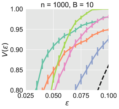
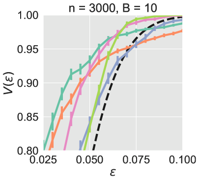
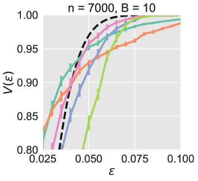
Figure 4: Marginal validity plots comparing UMD to other binning methods. The performance of UMD improves at higher values of $n$ and $\varepsilon$, and the performance of UMD is closely explained by its theoretical guarantee. Isotonic regression and fixed-width binning perform well at small values of $\varepsilon$.

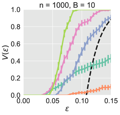
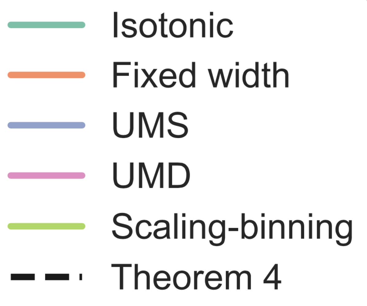
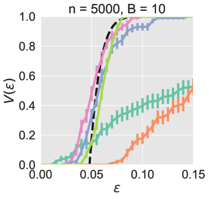
Figure 5: Conditional validity plots comparing UMD to other binning methods. UMD and scaling-binning are the best methods for conditional calibration at nearly all values of $n,\varepsilon$. Scaling-binning performs slightly better for small $n$ whereas UMD performs slightly better for large $n$. The performance of UMD is closely explained by its theoretical guarantee.

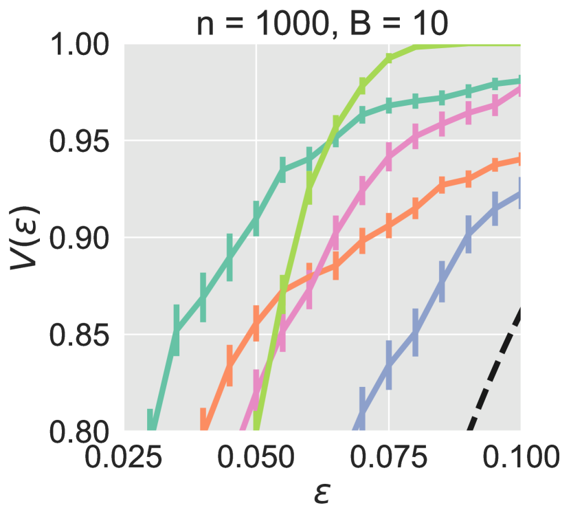
(a) Marginal validity plot.

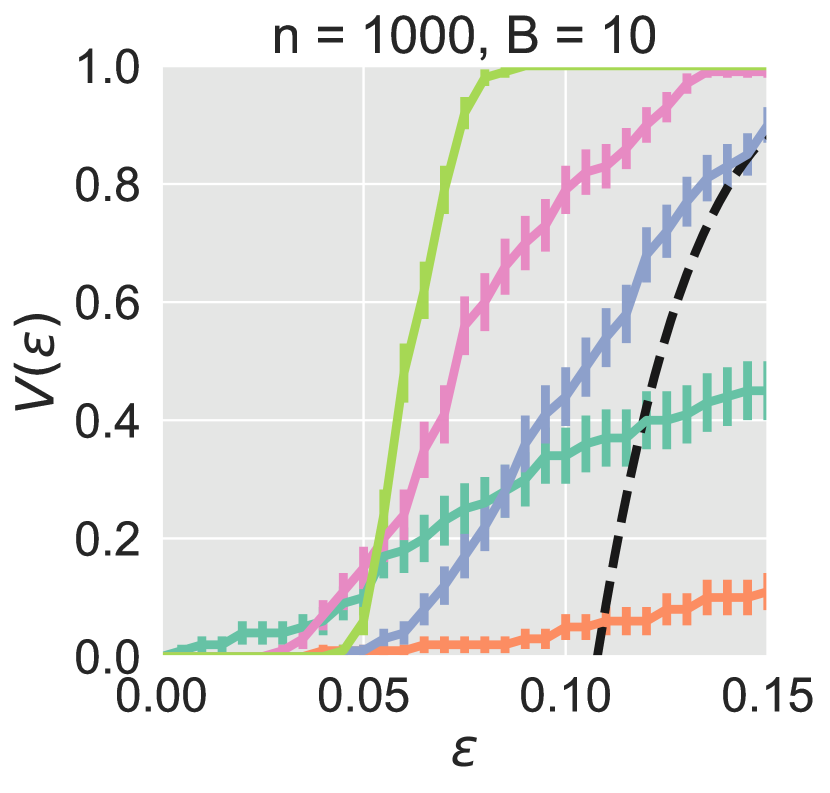
(b) Conditional validity plot.

Figure 6: Validity plots comparing UMD to other binning methods with fewer points used for recalibration. Namely, 14K points are used for training logistic regression, 1K for Platt scaling, and 1K for binning. Overall, scaling-binning performs quite well, since it relies on the underlying efficiency of logistic regression more than the other methods.

References

- Ahsanullah et al. [2013] Mohammad Ahsanullah, Valery B Nevzorov, and Mohammad Shakil. An introduction to order statistics, volume 8. Springer, 2013.
- Arnold et al. [2008] Barry C Arnold, Narayanaswamy Balakrishnan, and Haikady Navada Nagaraja. A first course in order statistics. SIAM, 2008.
- Breiman [2001] Leo Breiman. Random forests. Machine learning, 45(1):5–32, 2001.
- Bröcker [2012] Jochen Bröcker. Estimating reliability and resolution of probability forecasts through decomposition of the empirical score. Climate dynamics, 39(3-4):655–667, 2012.
- Clopper and Pearson [1934] Charles J Clopper and Egon S Pearson. The use of confidence or fiducial limits illustrated in the case of the binomial. Biometrika, 26(4):404–413, 1934.
- Dai et al. [2020] Ran Dai, Hyebin Song, Rina Foygel Barber, and Garvesh Raskutti. The bias of isotonic regression. Electronic journal of statistics, 14(1):801, 2020.
- Dawid [1982] A Philip Dawid. The well-calibrated Bayesian. Journal of the American Statistical Association, 77(379):605–610, 1982.
- Gneiting et al. [2007] Tilmann Gneiting, Fadoua Balabdaoui, and Adrian E Raftery. Probabilistic forecasts, calibration and sharpness. Journal of the Royal Statistical Society: Series B (Statistical Methodology), 69(2):243–268, 2007.
- Guo et al. [2017] Chuan Guo, Geoff Pleiss, Yu Sun, and Kilian Q. Weinberger. On calibration of modern neural networks. In International Conference on Machine Learning, 2017.
- Gupta et al. [2020] Chirag Gupta, Aleksandr Podkopaev, and Aaditya Ramdas. Distribution-free binary classification: prediction sets, confidence intervals and calibration. In Advances in Neural Information Processing Systems, 2020.
- Hébert-Johnson et al. [2018] Ursula Hébert-Johnson, Michael Kim, Omer Reingold, and Guy Rothblum. Multicalibration: Calibration for the (computationally-identifiable) masses. In International Conference on Machine Learning, 2018.
- Kull et al. [2017] Meelis Kull, Telmo M. Silva Filho, and Peter Flach. Beyond sigmoids: How to obtain well-calibrated probabilities from binary classifiers with beta calibration. Electronic Journal of Statistics, 11(2):5052–5080, 2017.
- Kumar et al. [2019] Ananya Kumar, Percy S Liang, and Tengyu Ma. Verified uncertainty calibration. In Advances in Neural Information Processing Systems, 2019.
- Lakshminarayanan et al. [2017] Balaji Lakshminarayanan, Alexander Pritzel, and Charles Blundell. Simple and scalable predictive uncertainty estimation using deep ensembles. In Advances in Neural Information Processing Systems, 2017.
- Lugosi and Nobel [1996] Gábor Lugosi and Andrew Nobel. Consistency of data-driven histogram methods for density estimation and classification. Annals of Statistics, 24(2):687–706, 1996.
- Miller [1962] Robert G Miller. Statistical prediction by discriminant analysis. In Statistical Prediction by Discriminant Analysis, pages 1–54. Springer, 1962.
- Naeini et al. [2015] Mahdi Pakdaman Naeini, Gregory Cooper, and Milos Hauskrecht. Obtaining well calibrated probabilities using Bayesian binning. In AAAI Conference on Artificial Intelligence, 2015.
- Niculescu-Mizil and Caruana [2005] Alexandru Niculescu-Mizil and Rich Caruana. Predicting good probabilities with supervised learning. In International Conference on Machine Learning, 2005.
- Parthasarathy and Bhattacharya [1961] KR Parthasarathy and PK Bhattacharya. Some limit theorems in regression theory. Sankhyā: The Indian Journal of Statistics, Series A, pages 91–102, 1961.
- Platt [1999] John C. Platt. Probabilistic outputs for support vector machines and comparisons to regularized likelihood methods. In Advances in Large Margin Classifiers, pages 61–74. MIT Press, 1999.
- Provost and Domingos [2003] Foster Provost and Pedro Domingos. Tree induction for probability-based ranking. Machine learning, 52(3):199–215, 2003.
- Roelofs et al. [2020] Rebecca Roelofs, Nicholas Cain, Jonathon Shlens, and Michael C Mozer. Mitigating bias in calibration error estimation. arXiv preprint arXiv:2012.08668, 2020.
- Sanders [1963] Frederick Sanders. On subjective probability forecasting. Journal of Applied Meteorology, 2(2):191–201, 1963.
- Widmann et al. [2019] David Widmann, Fredrik Lindsten, and Dave Zachariah. Calibration tests in multi-class classification: a unifying framework. In Advances in Neural Information Processing Systems, 2019.
- Yeh and Lien [2009] I-Cheng Yeh and Che-hui Lien. The comparisons of data mining techniques for the predictive accuracy of probability of default of credit card clients. Expert Systems with Applications, 36(2):2473–2480, 2009.
- Zadrozny and Elkan [2001] Bianca Zadrozny and Charles Elkan. Obtaining calibrated probability estimates from decision trees and naive Bayesian classifiers. In International Conference on Machine Learning, 2001.
- Zadrozny and Elkan [2002] Bianca Zadrozny and Charles Elkan. Transforming classifier scores into accurate multiclass probability estimates. In International Conference on Knowledge Discovery and Data Mining, 2002.