Symmetry Protected Quantum Computation
Abstract
We consider a model of quantum computation using qubits where it is possible to measure whether a given pair are in a singlet (total spin ) or triplet (total spin ) state. The physical motivation is that we can do these measurements in a way that is protected against revealing other information so long as all terms in the Hamiltonian are -invariant. We conjecture that this model is equivalent to BQP. Towards this goal, we show: (1) this model is capable of universal quantum computation with polylogarithmic overhead if it is supplemented by single qubit and gates. (2) Without any additional gates, it is at least as powerful as the weak model of “permutational quantum computation” of Jordan [M05, ]. (3) With postselection, the model is equivalent to PostBQP.
Imperfect physical gates are a major challenge for building a scalable quantum computer. One possible way to overcome this challenge is to use error correcting codes to build high fidelity logical gates from the lower fidelity physical gates [10]. Another approach is to use a topologically ordered state to store and manipulate quantum information, directly obtaining good logical gates [Kitaev_2003]. Here, we propose a third approach, to protect the operations by symmetries of the physical Hamiltonian.
In particular, we consider qubits encoded in quantum spins, and we assume that the Hamiltonian and any noise terms respect an symmetry acting on all the qubits simultaneously. We need a quick introduction into the representation theory of . The irreducible representations of are indexed by a quantity , called the spin. The dimensionality of a representation of spin is . The spin- representation has dimension , so can be regarded as a qubit. The tensor product of two spin- representations is the direct sum of a spin and spin representation. The singlet state of a pair of qubits is, up to an arbitrary phase, , while states in the subspace orthogonal to the singlet state are called triplet. The singlet state is anti-symmetric under exchange of qubits, while the triplet states are symmetric.
In the idealized case, a single qubit is not subject to any noise of any kind, since there are no terms that we can write down which are invariant under on that qubit. If we bring a pair of qubits together, then the total spin (either or ) is the only -invariant term on both qubits. Thus, dephasing may happen between spin (singlet) and spin (triplet) states; however, it also becomes possible to measure this total spin.
Our focus in this paper is on the power of these singlet/triplet measurements in an idealized model. To state our physical model: we assume that there are qubits for some , initially in some state which is a tensor product of singlets. We then allow arbitrary pairs of qubits to be selected and the total spin of those two qubits to be selected. We use the notation to indicate this operation, which projectively measures a pair of qubits to be in either the singlet () or triplet () subspace. From this physical model, we define a computational complexity class that we call STP, where a sequence of polynomially many such measurements is allowed. More precisely,
Definition 1.
STP is the class of problems that can be correctly answered, with constant probability larger than , using polynomially many measurements where the sequence of measurements to make is determined by a polynomial time classical algorithm based on the input string and on the previous measurement outcomes. Similarly, the decision of whether the input string is accepted or rejected is also determined by a polynomial time classical algorithm based on the string and the measurement outcomes.
As perhaps the “smallest” physical example where this can be realized, imagine a single electron and a single proton far separated from each other. Each has spin , and (assuming no magnetic fields are present and assuming that spin-orbit coupling can be ignored which depends on the electric fields and on the orbital degrees of freedom) then these spins are not subject to any decoherence. If the electron and proton are brought near each other, then there is a hyperfine coupling between these spins, and the ground state splits into singlet and triplet levels with slightly different energies which can in principle be measured. One might then try to compute by having a large number of electrons and protons and occasionally bringing a single electron near a single proton and measuring the total spin. This simple example is slightly different from the idealized model above, as some of the qubits are associated with electrons and some with protons, and pairs must have one electron and one proton.
More realistic examples include trapped ions where interaction between ions may be dependent on total spin, or spin blockade in quantum dots [13].
This paper considers the question: what is the computational power of STP? We believe the study of such a simple model, in addition to its symmetry protection, is of interest itself and we conjecture that STP is equivalent to BQP. Even if our conjecture is wrong and STP falls somewhere between P and BQP, the study of STP is still well-motivated as it is so distinct from other quantum computational models. While we do not show STP = BQP, we present several partial results111After this paper appeared, it was shown that STP=BQP [rudolph2021relational], building on [Rudolph_2005]. Even given that STP=BQP, the constructions here are of interest as they may give a lower overhead way to implement BQP in practice using additional approximate gates..
We emphasize that this kind of physical protection by symmetry is distinct from the approach using measurement based quantum computation in a symmetry-protected topological phase [Nautrup_2015].
First, in Section 1, we show how to implement universality using measurements as well as certain single qubit Cliffords and Pauli measurements. Our discussion will be in reverse order of the number of single qubit operations we allow: we will start with the full single qubit Clifford group and all Pauli measurements, and gradually reduce the number of single qubit operations required, until what is required is Clifford operations in addition to measurements. A related previous result is that operations combined with a source of many copies of three different states whose Bloch vectors span is also universal [Rudolph_2005]; s/t operations are used to purify mixed states and build any pure state, which are then used to build cluster states. This purification result, impossible to do using Clifford operations, further motivates the study of STP. We refer to the introduction in [Rudolph_2005] for further motivation behind the study of STP.
In Section 2, we show that STP is at least as powerful as the model of “weak permutational computing” [] (it has been shown [12] that there is an efficient classical algorithm to compute amplitudes in this permutational computing model, but no classical algorithm is known to solve the sampling problem in this model).
In Section 3, in line with our investigation of STP, we consider generalizations of STP, showing that allowing higher spin qudits does not increase the power of the model.
Finally, in Section 4, we define a postselected version of STP, called PostSTP, and show that it is equivalent to PostBQP. This implies that efficient exact sampling from an STP protocol is impossible assuming the polynomial hierarchy is infinite [11, See “Sidebar: The Polynomial Hierarchy and Post-Selection”]. An approximate efficient sampling, related to quantum supremacy experiments, is discussed in LABEL:statsofampsappendix (LABEL:STSampleproblem). Showing PostSTP = PostBQP does not imply STP = BQP, as there are other models, such as boson sampling and IQP which are not believed to be BQP and yet their postselection version equals PostBQP (see [11] for more on PostBQP and quantum supremacy experiments).
There are several interesting open questions, such as the obvious question of the hardness of sampling measurement outcomes for some sequence of measurements, with the sequence randomly chosen or chosen in some other way.
A final result that may be of independent interest is given in LABEL:irrmeasure, namely a relation between the “irrationality measure” of an irrational angle and how many times one may need to rotate by that angle to approximate some desired target angle to some desired accuracy. Although we use this result in Section 1.1.2, it is only to show an efficient approximation that can also be done with more elementary facts. Likely the result in LABEL:irrmeasure is well-known, but since we did not find it elsewhere we record it here.
1 and is Universal for Quantum Computation
We show that:
Theorem 1.
Using measurements, and single qubit unitaries, we can approximate a gate set consisting of one and two qubit Clifford operations and Pauli measurements, as well as gates, with an expected overhead that is only polylogarithmic in the error in this approximation.
Remark 1.
The polylogarithmic overhead arises for a familiar reason: we will exactly implement Clifford gates and then implement gates by magic state distillation using as input approximate gates that we can form from the given operations. The overhead scales polylogarithmically in the accuracy of the distilled gates. The implementation of the circuit is probabilistic, as certain operations are repeated until they succeed, which is why the theorem refers to an expected overhead.
1.1 and Single Qubit Clifford and Pauli Measurement is Universal for Quantum Computing
We first show that on arbitrary pairs of qubits, combined with arbitrary Cliffords on a single qubit (i.e., ) and single qubit Pauli measurements, is universal for quantum computing. In particular, we can approximate a gate set consisting of one and two qubit Cliffords operations and Pauli measurements, as well as gates, with an overhead that is only polylogarithmic in the error.
In subsequent sections, we reduce the number of single qubit operations required at the cost of making the construction more complicated.
We begin by showing that we can implement the full Clifford group, and then show universality.
1.1.1 Implementing the Full Clifford Group
First, we prove:
Lemma 1 (Bell basis measurement).
We can implement a four outcome projective measurement on two qubits in a Bell basis:
Proof.
To do this, first apply an measurement. If the outcome is , then the qubits are in the first Bell state. If the outcome is , apply and again measure . If the outcome is , then the qubits were in the second Bell state. If the outcome is , apply and again measure ; if the outcome is , then the qubits were in the third Bell state. If the outcome is , then the qubits were in the fourth Bell state. ∎
Remark 2.
Since we can do Bell basis measurements, we can teleport: given a pair of qubits labeled in a Bell state, we can bring in an additional qubit labeled and measure in the Bell basis. This teleports the state of to , up to some correction on which is a single qubit Clifford.
Further, we can teleport more than one qubit, and use this to perform Clifford operations if we can prepare appropriately entangled states. To prove that for the case of CNOT, consider a state on four qubits obtained by taking in a singlet and in a singlet, and then applying a CNOT from to . We then bring in two extra qubits , and measure in the Bell basis and measure in a Bell basis. This teleports the state of to and then applies a CNOT, again up to some single qubit Cliffords on .
So, if we can prepare this state , then we can perform CNOT operations. Combined with the ability to perform single qubit Cliffords, this gives the full Clifford group. It seems at this point that we are trying to get a “free lunch”: the most obvious way to prepare is to perform a CNOT operation, which is precisely the operation we are trying to produce.
However, it is possible to prepare using just and single qubit Cliffords, as we now show. First we construct a double spin operation .
Lemma 2 ().
We can produce an operation which acts on a pair of qubits and projectively measures and, if , then it also measures .
Proof.
To do this, simply perform only the first two measurements of the protocol above to measure in the Bell basis: if either of the first two measurements are , then and we have also measured . If both measurements are , then but no other information is revealed; we should then apply to undo the first application of . ∎
Corollary 1 ().
Using the operation , it is possible to produce an operation which always measures and, with probability , also measures .
Proof.
To do this, flip an unbiased coin: if it is heads, apply ; if it is tails, apply , then apply , then apply again. Then, if we measure if the coin is tails but not if it is heads, while if , we measure if the coin is heads but not if it is tails. ∎
Remark 3 ().
Similarly, we can produce an operation which measures and, if , also measures , and we can produce an operation which measures and, with probability measures otherwise measuring nothing else. To construct , we use the same construction as except we apply after the first measurement if the result is , rather than applying . We construct similarly. Also (we will use this in Section 1.2.2), we can produce operations and . To construct , we apply (up to scalar phase) after the first measurement if it is .
We will say that , succeed if they measure only without measuring additional information. Similarly, we say that (respectively, ) succeed if they measure only (respectively, ) without revealing any additional information.
Lemma 3 (CNOT).
We can produce a CNOT gate using an ancilla, given the ability to perform single qubit Cliffords and Pauli measurements as well as to apply on an arbitrary pair of qubits.
Proof.
The circuit [Xue_2013, Karzig_2017] is: prepare the ancilla in the state, measure on the source and ancilla, measure on the ancilla and target, and finally measure on the ancilla, and apply single qubit Clifford corrections if needed. The original reference [Xue_2013] writes the circuit with additional Hadamard gates so that all measurements are or , but it conjugates to the circuit we give here.
Now, to produce the CNOT gate action, recall that we only need to prepare the state . We do so by a probabilistic protocol: prepare two entangled qubits. Then, attempt to produce a CNOT gate by using operations and in place of the and measurements in the aforementioned protocol for a CNOT. If both and succeed, we have produced the desired . If one does not succeed, we may simply try again.
∎
Remark 4.
Note that in this probabilistic protocol, indeed and will each succeed with probability , without any need to use and .
Thus, this protocol to perform a CNOT gate can be understood simply as, first, we have a protocol that sometimes succeeds in performing the desired CNOT, and, second, by preparing entangled states “offline”. Offline operations use expendable qubits where, without any loss in efficiency, we can start again the operations/measurements on new qubits if the desired result was not obtained. This is in contrast to online operations applied on the data (computational+ancilla) qubits. By teleporting through the entangled states, we can use this to perform CNOTs on data qubits by “only using the CNOT when it will succeed”.
1.1.2 Universality
Now we show universality. The construction here is not intended to be optimal in terms of minimizing overhead in any way. It is simply intended to be a simple way to show universality by leveraging standard results.
Lemma 4.
We can prepare (offline) a non-stabilizer pure state on a single qubit.
Proof.
Prepare two qubits in states and using measurements and applying if the wrong outcome occurs. Project into the triplet state (if instead they are in a singlet, re-prepare and try again). The result is, up to normalization, . Measure the second qubit in the basis; we assume without loss of generality that the result is . The result state on the first qubit is, up to normalization, . With normalization this is , where is an irrational angle [2]. ∎
Any such state is equal to . Using this as a resource for state injection produces a rotation by
where the sign is chosen uniformly at random (our basis for state injection is a little different from the standard one since we rotate by instead of by ). This state injection can be done, e.g., as in [4, Section III] by modifying the following appropriately using a Hadamard and phase gate:
| (1.1) |
where is a -measurement on the second qubit, and the controlled rotation . Note that , with the Hadamard and phase gate. We shall address the issue of sign in shortly.
In the simplest applications of state injection, one imagines a situation where rotation by twice the angle is available as a primitive (for example, using state injection to produce gates and assume that one has gates available). In that case, if the sign is not what one wants, one can recover with a rotation by twice the angle. We do not have that option here.
We use a different approach. Pick any desired target angle , and any error . Then, repeatedly apply state injection (like in Eq. 1.1) to a qubit initialized in the state, until the result is where for some and
Here, when we apply state injection, we do not care whether the plus sign or minus sign is chosen. The result is some random walk in angles and since is irrational, in expected time , where is the irrationality measure of (LABEL:irrmeasure), we get .
Choosing , we can then produce states arbitrarily close to a magic state for a rotation by , i.e., a magic state for a “” gate, where the quotes are because this is rotation by rather than . Choosing sufficiently small, one can then use this gate as input into any standard gate distillation protocol (like in Eq. 1.1 but for ) [4, Section III] to obtain universality with only polylogarithmic overhead in the target error.
1.2 Reducing the Single Qubit Operations Needed
We now reduce the single qubit operations required.
1.2.1 Avoiding Use of Hadamard and gates
First, we note that it is possible to avoid using both Hadamard and gates. Without these gates, our construction of Section 1.1.1 gives the subgroup of the Clifford group generated by single qubit and and two qubit CNOT. Call this subgroup . We now show that we can generate the full Clifford group using just , and single qubit Pauli measurements.
Lemma 5.
The Hadamard and phase gates can be derived by using gate distillation with the help of and single qubit Pauli measurements.
Proof.
Since we can measure single qubit Paulis, prepare qubits in state . Using these qubits as a target for state injection for rotations by , we can produce the gate. This state injection protocol requires only , and CNOT gates and single qubit Pauli measurements, so it requires only the subgroup above. Note that since we have the single qubit available, we can recover state injection if we instead produce (Eq. 1.2).
| (1.2) |
We can also use the same state in state injection to produce rotation by (Eq. 1.3). To do this we use the usual state injection protocol, except we interchange the control and target on the CNOT gate in state injection, and we replace the final measurement in state injection with an measurement. The effect of this is to perform state injection in a Hadamard basis (even though no Hadamards are used!), since is equal to a CNOT gate with control and target interchanged.
| (1.3) |
Combining rotations , we can produce the full single qubit Clifford group, including . ∎
1.2.2 and is Universal
Let us now show finish the proof of Theorem 1 by showing:
Lemma 6.
Single qubit Pauli measurements can be derived using and .
Proof.
Recall that using just and , we have a protocol which measures on any two qubits and which measures nothing else with probability . So, imagine that we have a set of qubits such that the product for all pairs of qubits in . Consider another qubit in any state. Then, pick any qubit from and measure . With probability nothing else is measured and if , we can add to the set; if , we can apply to and then add to the set. On the other hand, with probability , additional information is measured; in this case, we remove from .
So, with probability , and with probability , . This allows us to build up large sets . Since the size of does an unbiased random walk, it takes operation to produce a set with . We can then use such a set as a “standard”: throw out any qubit in . The remaining qubits are then in a state which is an incoherent mixture of and .
So, let us analyze these two cases, where the remaining qubits are either in or , separately. First suppose that the state is . Call each of these qubits “ standards”. Then, any time we want to measure on a single qubit, we get a standard and use to measure on the given qubit and the standard. If we measure no other information other than , we can now in fact use both qubits as standards; if we also measure , we discard both qubits. So, at most one standard is consumed per measurement. Note that even if does not succeed, so that we also measure , we still have learned the value of on the given qubit: the effect is to measure the value of on the given qubit and then bring that qubit and the standard into a Bell pair.
We assumed that the standards were in the state . If instead they are in the state , nothing changes: our labels and are arbitrary and can be interchanged. This is a consequence of a symmetry of our operations , which are invariant (up to an unobservable phase) under conjugation by . Indeed, if our labels were not arbitrary, then some sequence would reveal the difference between these two states, in which case we could, assuming we had , apply to every qubit to obtain .
So, we can measure single qubit with a quadratic overhead: the number of operations is proportional to the square of the number of measurements. Similarly, we can measure single qubit and single qubit by preparing standards (respectively, standards), which are sets of qubits where (respectively, ) for every pair in the set. This finishes the proof of the lemma and as a result Theorem 1. ∎
Remark 5.
In fact, the quadratic overhead can easily be reduced to linear. Suppose we have some such set . In operations we can prepare another set with such that all pairs of qubits in also have . Then, pick one qubit from and one from and apply . If this succeeds with , add all qubits from to and if it succeeds with , apply to all qubits in and then add all qubits in to . If it fails, remove the given qubit from and discard . Thus, with probability with have , while with probability we have .
This gives a biased random walk in and so increases linearly in the number of operations with high probability. We leave it to the reader to consider optimizing the linear increase. For example, what is the best to use; should one in fact apply this construction recursively by constructing using a similar process; one can in fact avoid discarding all of but only discard the measured qubit if does not succeed and so on.
2 Permutational Quantum Computation
For any binary tree with leaves, we define a set of commuting operators on a system of qubits. Each qubit corresponds to one leaf. For every vertex (including the root), there is an operator with eigenvalues corresponding to the total spin of the qubits corresponding to leaves which are descendants of that vertex. Additionally, for the root, there is another operator with eigenvalues corresponding to the total spin in the -direction of the qubits, denoted .
The eigenvalues of these operators (all together forming a tuple of half-integers) define a complete eigenbasis. We say that a labelled tree is a binary tree with labels at each vertex (Fig. 2.1), with the labels at each vertex being chosen from the set of eigenvalues of the operator(s) corresponding to that vertex. We use to denote unlabelled binary trees (Fig. 2.2). We use to denote labeled binary trees, and use to denote the corresponding states.
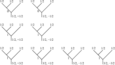

There are two models of permutational quantum computing. In the weak model, one can prepare any state corresponding to any labelled tree. One can then pick any any other tree and projectively measure the corresponding operators for that tree. If is a labeling of , then one can measure to inverse polynomial accuracy by repeating this projective measurement polynomially many times. In the strong model, we assume that one can also measure (without taking the absolute value) to inverse polynomial accuracy. While this problem of computing can be done classically [12], there is no known efficient classical algorithm for the problem of sampling from with probability .
We show that:
Theorem 2.
Using just , one can simulate the weak model in polynomial time.
2.1 Reducing to case that root has spin
First note that it suffices to consider the case that the root has spin . The reader may prefer to skip this section on first reading.
Indeed, consider any such that has spin . Introduce notation: let be a state defined by some labeled tree with the -spin at root replaced by . Then, unless and . Fix some unlabelled tree . To sample with probability , we do the following. Adjoin an additional ancilla qubits, defining some tree which constrains those ancillas to be in the spin state (there are many possible such as all we care about is the root spin; choose an arbitrary such ). Then join the root of to the root of to produce222The root of has two labels, since it also has a label by some . This root becomes an internal vertex of which should have only one label. We drop the label when we build . some with spin . Let be an unlabelled tree, obtained by removing the labels from . Join the root of to to produce some . Then, prepare and projectively measure the eigenvalues corresponding to tree . Note that we will always measure . This projective measurement gives a labeling of , which induces a labeling of since is contained in (we can assume that the root of has since otherwise the amplitude is zero).
We claim that this correctly samples the amplitudes. That is, if is a labeling of , which induces some labeling of , then is equal to . To see that this, note that
where are some Clebsch-Gordan coefficients. Do the same expansion for and then
Since the inner product on the right-hand side is independent333 We show this here. Let (in a slight overuse of notation) denote the sum of Pauli operators on all qubits. The state is a superposition of states with different . The inner product is independent of and by expanding in it follows that is independent of the particular . of , the result follows.
2.2 Measuring operators for some tree
Next we describe how to projectively measure operators corresponding to any tree with root having total spin . The key is that given any set of qubits with for some , we can approximately measure the total spin of those qubits as follows. Simply repeat the following operation many times: choose a random pair of qubits, and measure . We show below that the number of measurements needed is at most inverse polynomial in the accuracy.
Then, letting denote the squared spin, and denote a vector of spin operators (one-half the Pauli operators) on qubit ,
| (2.1) |
Hence, averaging over randomly selected , the expectation value of equals . In a triplet state, while in a singlet it equals . So, the probability of triplet is
Note that while this measurement of singlet or triplet may change the state of the qubits in , it does not change the total spin and since we randomly choose each time, the probability of triplet depends only on the total spin. Hence, since the measurements are independent, we may estimate the spin in a time which is inverse polynomial in the accuracy. Indeed, since the spin is quantized, the convergence is actually faster than polynomial. Once the number of measurements is polynomially large compared to , the convergence in accuracy becomes exponential444This fact was used in [rudolph2021relational] for the STP=BQP proof..
Using this ability to measure total spin of a set of particles as a primitive, we can measure the operators corresponding to any tree . The key is to start at the leaves and work towards the root. Measure operators corresponding first to vertices closest to the leaves. Proceed toward the root, only measuring an operator on a given vertex once all operators below that vertex have been measured.
The point is, that while the operators corresponding to different vertices commute with each other, our measurement process reveals extra information. Our measurement process need not commute for different vertices. However, our measurement process for a given vertex does not affect the total spin on vertices closer to the root.
2.3 Preparing states
We now explain how to prepare a state in polynomial expected time. In this case, we work in the reverse direction: we start at the root and work towards the leaves. In particular, we will prepare a sequence of states . This corresponds to a sequence of partially labeled trees . In a partially labeled tree, some set of vertices will have labels, and if a vertex is labeled, then all vertices which are ancestors of will also be labeled. The partially labeled tree will have the root labeled with and no other labels. Each tree will have two more vertices labeled than the previous tree in the sequence; this will be done by labeling a pair of vertices which are children of some vertex which is labeled in , and the last tree in the sequence will have all vertices labeled and will be the same as .
Each state corresponding to some partially labeled tree will have the property that for every operator corresponding to a labeled vertex of , the state will have the corresponding expectation value for that operator. No other properties of the state are assumed, so a partially labeled tree does not uniquely specify a state.
Preparing the first state is easy: one may simply create any choice of singlets. We will construct a primitive operation that we call splitting which has the following properties. 1: The splitting primitive takes as input a set of qubits with total spin for some ; there are no other assumptions on the input state. 2: One fixes some and some with . 3: The splitting primitive applies measurements to qubits from that set, taking polynomial expected time. 4: The resulting state has (up to exponentially small error) the first qubits with total spin and the remaining qubits with total spin .
Given this splitting primitive, we can then produce each state from the state , by applying splitting to the set of qubits corresponding to descendants of , with depending on the labels in for the children of .
We now construct the splitting primitive above. First, let us say that a set of qubits with total spin are in canonical form if there are singlet pairs (in some fixed configuration, rather than a superposition) and the remaining qubits are in a totally symmetric state. For example, a state on qubits with qubits in an singlet and in a singlet and in a totally symmetric state is in canonical form.
We divide the construction of splitting into four steps.
First Step— First, we take the qubits and bring them to canonical form. The construction is recursive. If , then they are already in canonical form. If not, pick a pair of qubits at random and measure . If the result is triplet, pick another pair at random, and try again, continuing until eventually some pair is in a singlet. That gives one singlet; we then bring the remaining qubits to canonical form using the same algorithm recursively. This takes polynomial expected time.
Second Step— Recall that we wish to divide the set of qubits into two sets, with and qubits respectively, and with total spin and , with . Let . Let and be the two values for total spin such that and .
Our second step will be to take the state after the first step which is already in canonical form, and divide it into two sets of qubits, of sizes respectively, with total spins and respectively, with each set in canonical form. Call these two sets and . This division can be done easily: take the qubits in a totally symmetric state, and place qubits in and the remaining in . Then, take the singlets from the state in the first step, and place each singlet into one of the two sets (either or ), so that the total sizes of the two sets are correct.
Third Step— Our third step acts only on certain subsets of sets . We call these subsets and both have size . These subsets are given by choosing singlets from and letting those be in and choosing singlets from and letting those be in . Qubits will remain in the subset they are in after the second step, but their state will change due to this step. What the step will do is bring it to a state where those qubits are now in a totally symmetric state in each set individually (i.e., the qubits in are totally symmetric, as are the qubits in ), while the total spin of those qubits is still .
To do this, we use an iterative algorithm. First, A: bring both subsets into canonical form. If there are no singlets in either one, terminate. Otherwise, B: if either subset has a singlet, then so must the other555This is because the total spin of qubits in is . If has at least one singlet, then has total spin less than the maximal value of and so must also have total spin less than in order for total spin of to be .. Pick a pair of qubits, one from a singlet in each subset, and measure . Call these qubits and call the singlets that they are in respectively . Then, regardless of the measurement outcome, measure on both qubits in . If the result is , this pair of measurements has had no effect on the spins; in this case repeat the pair of measurements, continuing until the second measurement give . Once the second measurement gives , go back to step A.
We claim that this takes polynomial expected time. Consider the effect of B. Suppose that before measuring B the total spin in each set was . After B, the total spin in each set must be one of the possibilities . The total spin squared666We remind the reader that the spin squared is , not . before B is and the total spin squared after B has expectation value . The process of bringing into canonical form measures the total spin in each set. We claim that the probability that the total spin squared is is greater than the probability that it is . Indeed, this must follow in order for the total spin squared to have expectation value after B because
Hence, the total spin does a biased random walk with the bias toward increasing spin, and so the spin must become maximal in at most polynomial time.
Fourth Step— After the third step, we have the following. Each of the two sets has three subsets. Let denote the three subsets of the first set and denote the three subsets of the second set, with comprising and comprising . The sets each contain qubits in some product of singlets. The sets and each contain qubits in a totally symmetric state, with the union of and having total spin . The sets and also each contain qubits in a totally symmetric state, but now the union of and is also in a totally symmetric state. In the fourth step, we act on sets and to try to bring them to a totally symmetric state (we also do the same procedure to and with the same goal but we just describe it for ). To do this, we we apply a large number of measurements on qubits randomly chosen from the union of and . If all measurement outcomes are , then the application of these measurements converges to projecting onto the state where those qubits in union are in a totally symmetric state of total spin and we succeed. The convergence to this projector is exponential, once one has more than polynomially many measurements.
The probability that all measurements are in this step is at least inverse polynomial. This may be seen by computing the projection of the initial state onto the space where are totally symmetric and are totally symmetric. If we fail, so that some measurement is , we repeat all steps of this process.
3 Generalizing the Model
The model STP can be generalized in several ways. One natural generalization is to consider symmetries other than , such as for . Another natural generalization is to consider higher spin representations of .
In such a higher spin representation model, we have qudits, for with integer or half-integer. We may consider having several different kinds of qudits simultaneously, for example having both qubits () and qutrits (). We allow any two qudits (perhaps of different dimensions) to be brought together, and the total spin to be measured.
As a toy physical example, one might imagine deuterium. The deuterium nucleus has total spin , while the electron has spin . The deuterium atom then has total spin or and there is a hyperfine splitting between these states.
Interestingly, this higher spin model can be simulated using just on qubits. To simulate a qudit with spin , use qubits in a totally symmetric state. When two qudits with spin are brought together, we can measure the total spin of the qubits by repeatedly selecting pairs of qubits uniformly at random and measuring . Exactly as in Section 2, the convergence in accuracy is exponential once we have a number of measurements which is polynomial in the total spin.
After measuring the total spin, we can then bring the qubits into two sets of qubits respectively, both in a totally symmetric state, again as in Section 2. Indeed, this is done by the splitting primitive.
4 PostSTP Equals PostBQP
Let us formally define STP with postelection.
Definition 2.
Let PostSTP be the class of languages such that for all inputs the following holds. A quantum state is initialized as a product of polynomially many singlets. Then some classical algorithm (determined by ) takes as input and outputs a sequence of polynomially many measurements (as well as outcomes to postselect upon for all but the last measurement), taking polynomial time to output this sequence. The sequence of measurements is applied to the input state. Postselection is applied on all but the last measurement, with the promise that the outcomes postselected on have nonzero probability. Finally, if , then the last measurement is with probability at least for some and if , then the last measurement is with probability at most for some strictly less than . The quantities are independent of input size.
Remark 6.
To define postselection in symbols, let be the product of singlets which is the initial state. Let be a projector which projects onto the desired outcome (either or ) of the -th measurement. Let be the product of these projectors up to the -th one. Let there be measurement outcomes that we postselect on, and let denote the projector onto the singlet outcome for the last (the -st) measurement. Then, the probability that the last outcome is is
where we are promised that the denominator is nonzero.
We will show
Theorem 3.
PostSTP equals PostBQP.
In outline, we prove this result by first showing in Section 4.2 that we can use postselection to simulate imaginary time evolution with Heisenberg interactions. Ref. [5] showed that approximating the ground state energy of Hamiltonian with Heisenberg interactions is QMA-hard (see also [6]), so this shows already PostSTP is at least as powerful as QMA: simply evolve under the desired Heisenberg Hamiltonian for a polynomially long imaginary time. To show that we get PostBQP, we use the ability to produce evolution “time-dependent” Heisenberg interactions in imaginary time, i.e., to vary the Heisenberg Hamiltonian that we evolve under. We use the same encoding as in [5] to show in Section 4.3 that this gives us PostBQP. Appropriate choices of time-dependent Heisenberg Hamiltonians will give us both circuits and measurement. We will have to pay some attention to making errors exponentially small when we do this.
Before doing this, we show in Section 4.1 that the probabilities that we postselect on can only ever become exponentially small in .
4.1 A Remark On How Small Amplitudes Can Become
Let be the product of singlets which is the initial quantum state for PostSTP.
We show
Lemma 7.
The nonzero probabilities that can occur in PostSTP are all .
Proof.
The probability that the -th measurement outcome has the desired value is
Clearly, the denominator is at most . So, we lower bound the numerator.
Note that every postselection can be replaced by , where is the gate that swaps a pair of qubits. Similarly, every postselection can be replaced by . Hence, the numerator is the sum of different terms, corresponding to replacing individual projectors by either the identity or . The contribution of any such term to the expectation value is of the form , where is the composition of some SWAPs, hence some permutation to the qubits. Recall that is the product of singlets, and therefore it is easy to see that for any permutation Permute of the qubits, the expectation value is for some . So, the expectation value is a sum of different terms, each of which equals , for some depending on the permutation Permute. Hence, if nonzero, the expectation value is at least , where . ∎
4.2 Simulating Imaginary Time Evolution
Let be the four qubit state, on four qubits called , with total spin given by first preparing in a singlet and in a singlet and then acting with , and finally appropriately normalizing the state to unit norm.
Now consider the effect of bringing in two extra qubits in some arbitrary state , and postselecting on being and on being . One may commute the postselection on and being in with the action of used to define . So, the effect of this operation is to teleport the state to qubits , while leaving and in singlets.
So, if we can produce , we can apply the operation . Of course, the ability to apply correspondingly implies the ability to create . Thus, the two things (the state and the operation) are equivalent as resources.
Note that the projection onto is given (up to normalization) by the operation with , so we can create .
We will give a protocol to reduce , consuming a pair of states with given and applying the operation to an arbitrary pair of qubits , with
| (4.1) |
If were in a singlet initially, this creates . By applying this protocol repeatedly, we can produce a sequence of states with and
Remark 7.
Of course we could also start with which projects onto up to normalization, but this does not lead to anything interesting.
The protocol is as follows. Create a pair of qubits in a singlet, and let be arbitrary. Then, apply , consuming the two copies of to do this, and again project onto in a singlet. A little algebra shows that the resulting state (up to normalization) is a singlet on and the operation is applied. We emphasize that Eq. 4.1 is not a perturbative result for small , but rather holds for all .
The cost of applying the -th operation, , is exponential in . At the same time, the magnitude of decreases doubly-exponentially in , roughly squaring at every step. So, for any , we can construct the operation for some in the interval using a number of operations at most logarithmic in : simply search for the first term in the sequence which lies in this interval.
To obtain operations with negative , consider a slight modification of the above sequence of operations. Create a pair of qubits in a singlet, and let be arbitrary. Apply , and again project onto in a singlet, with and from the above sequence. So,
Lemma 8.
For any and any , we can construct the operation for some with , using a number of operations at most .
Proof.
Construct for some which has the same sign as , with sufficiently small compared to , but not much smaller than , i.e. . Then, take powers of this operation to obtain a suitable . Since is not much smaller than , it takes at most operations to do this. ∎
Remark 8.
When constructing powers of the operation, it is more convenient to work with an exponentiated form of the operation: , where depends on .
Remark 9.
Likely the dependence of the number of operations on can be greatly reduced. We have given an inefficient construction that involves first constructing an operation with a very small and then taking powers of that operation. One might instead apply operations with several different with different magnitudes to reduce the total. We do not worry about that here.
So,
Lemma 9.
In PostSTP, we can approximate imaginary time evolution under a time-dependent Heisenberg Hamiltonian, up to inverse polynomial error.
The proof of this lemma is immediate, once we define what we mean. A “Heisenberg Hamiltonian” means a Hamiltonian of the form where is some polynomially-bounded matrix. By imaginary time evolution under such a Hamiltonian, we mean evolving an initial state under the equation , up to normalization. By “time-dependent”, we allow where is some polynomially bounded matrix which depends on and we allow . Finally, the inverse polynomial error is an error on the right-hand side of the evolution equation: where is a state whose norm may be made polynomially smaller than .
Then, to prove the lemma, we simply Trotterize777The evolution can be efficiently approximated by the Lie-Trotter product formula for small enough. the imaginary time evolution equation, and simulate the Trotter steps using postselection by picking to be polynomially small in the state , and applying Lemma 8.
This already immediately implies that
Corollary 2.
PostSTP contains QMA.
Proof.
By [5], approximating the ground state of a Heisenberg Hamiltonian to inverse polynomial error is QMA-hard. The operator is a ground state projector and hence by approximating this imaginary evolution up to inverse polynomial error, we can estimate the ground state of this Hamiltonian. ∎
4.3 Simulating PostBQP
However, our goal is not just to prove that PostSTP contains QMA, but rather than PostSTP is equivalent to PostBQP.
To do this, we again use results from [5]. We use the result (see section 5.1 of that paper) that using Heisenberg interactions we can implement logical qubits (using three physical qubits for each logical) and obtain terms on any given logical qubit as well as terms on pairs (see also [7] for an encoding using the Heisenberg interaction). So, it suffices then to consider a model of computation in which we have qubits (which for the rest of this subsection refer to the logical qubits of [5]), and the ability to implement imaginary time evolution under time-dependent , up to inverse polynomial error. Throughout this subsection, when we refer to time, we mean imaginary time.
By turning on an term on a pair of qubits for a long time and then turning it off (while leaving other terms off), we can approximately project onto the or eigenstates, and similarly using terms we can approximately project onto or eigenstates. Further, by turning on a sum of and terms on a single qubit (while leaving other terms off), we can prepare an ancilla qubit in a state which is approximately any desired pure state .
These abilities suffice. First, we can approximately prepare a qubit in a state, and then using it as an ancilla, we can approximately apply a CNOT from a source to a target by using the ability to approximately postselect on and eigenstates. This is the same as we used in Section 1.1.1 from [Xue_2013, Karzig_2017]. Note importantly that here we are using imaginary time evolution to approximately apply a unitary gate. This should be not be surprising; after all, the well-known idea of measurement based quantum computation [Raussendorf_2003] uses a sequence of measurements to apply unitary gates.
Also, by preparing ancillas which are approximately in states for other choices of , and using the CNOT gates and state injection, we can approximately implement unitary rotations to produce approximate rotations by where is the single qubit Pauli .
The ability to do CNOT and rotations allows universal quantum computation. So, if we ignore issues of error (i.e., the fact that all our constructions only approximately gave these gates), we can implement arbitrary quantum circuits and further we can postselect on measurement outcomes since we can implement imaginary time evolution under , giving PostBQP.
The issue of error can be resolved by implementing a fault tolerant construction using these approximate gates. Note that the error in the gates can be made arbitrarily small. Indeed, we can even make the error in individual gates for any polynomial at the cost of a polynomial overhead, so we can make the error in gates polynomially smaller than the the inverse of the total number of gates! Thus, if our goal were simply to simulate BQP, where we would be satisfied with an inverse polynomial error in the output probabilities of our quantum circuit, there would be no need for any fault tolerance. However, since we want to simulate PostBQP, we need exponentially small errors. So, some fault tolerant construction is needed.
Of course, the ability to make the error in individual gates polynomially small compared to the inverse of the total number of gates certainly simplifies the fault tolerant construction. However, we claim that in fact the usual threshold theorems can be applied to our setting and so long as the error in individual gates is sufficiently small, we can make the error in logical operations exponentially small.
The usual threshold theorems involve replacing idealized unitary gates by CPTP maps that approximate (in diamond norm) the desired unitary operations. Instead, we are replacing idealized unitary gates by linear operators that act on pure states (rather than mixed states) that are close in operator norm to the desired unitary. However, we now show that the usual threshold theorems can be adapted to this case.
Consider any given gate in the circuit, which ideally would be implemented by some unitary we will call . Suppose instead we implement some map (which is a linear operator on pure state) with , where is the operator norm. Then, has singular values bounded by and if we define to be any operator such that then
is a CPTP map with two Krauss operators, .
Making such a replacement for all gates in the circuit, we get a “noisy circuit” where every gate has two Krauss operators, with the first Krauss operator being close to the ideal unitary. The usual threshold theorems apply to this noisy circuit for sufficiently small showing that the logical error is exponentially small. Then, the situation relevant for us is one in which every time a CPTP map is applied for some gate, we pick the first Krauss operator (that is, in this case), rather than the second. This can be physically thought of as selecting a particular noise pattern.
So, we ask: if we select the first Krauss operator for every CPTP map in the noisy circuit, is the error still exponentially small? Intuitively, there is no problem: the first Krauss operator is closer to what we want than the second Krauss operator, so the situation in which we select that Krauss operator every time should be even better than a random choice.
To prove this, of course one could reprove the threshold theorem, using our gates (which are not noisy in that they map pure states to pure states but which still only approximate the desired gates). Indeed, this could be done simply by following through some existing construction and showing that the error is exponentially reduced if the first Krauss operator is selected every time. However, we would like to minimize our effort, and show that the error is exponentially small using the standard threshold theorem as a “black box”, without delving into the proof. To do this, we use a simple trick. Use some hierarchical construction to prove the threshold theorem, see for example [10] for a review of various constructions. Using such a hierarchical construction of the threshold theorem, one considers codes of some size, and proves that each step of the hierarchy reduces the error rate. If the error rate is at some level, then it is for some at a higher level of the hierarchy and so for sufficiently small the error rate reduces. We regard this error rate as a sum over different trajectories, corresponding to different choices of Krauss operators in each CPTP map. The contribution of the trajectory where we select the first Krauss operator in every map is , with the constant hidden in the big-O notation depending on the size of the code. So, for sufficiently small , the contribution of the that trajectory is the dominant one and so the error rate for that trajectory at the next level of the hierarchy is also , i.e., the hierarchical construction reduces error rate for sufficiently small for this case as well.
Remark 10.
Ref. [6] shows how to simulate 2D topological phases from imaginary time Heisenberg evolution. Anyons may be built into these simulations as boundary conditions, and time dependence of the Hamiltonians allows these anyons to be braided adiabatically, and then, later, collective (topological) charge states to be measured by simulating interferometry. In other words, once one can build imaginary time Heisenberg evolution (as in Lemma 9), one can simulate the complete operation of a topological quantum computer. This provides an alternative path from Lemma 9 to showing that PostSTP equals PostBQP, the post-selection in the conclusion stemming from our ability to post-select measurement outcomes of the simulated topological quantum computer, and the topological protection of the state allowing us to make errors exponentially small. While this is an extremely concise argument in outline, some details regarding efficiency should be filled in; this is why we gave the more explicit argument first.
Acknowledgements
We would like to thank Dave Bacon for pointing out the relevance of [Rudolph_2005], and anonymous referees for helpful comments to improve our paper. The first named author would like to thank the Aspen Center for Physics for their hospitality. The third named author would like to acknowledge the support of the Perimeter Institute for Theoretical Physics and Microsoft. Research at Perimeter Institute is supported by the Government of Canada through Innovation, Science and Economic Development Canada and by the Province of Ontario through the Ministry of Research, Innovation and Science. The experiments were conducted using Microsoft computational resources.
References
- [1] MathOverflow discussion.
- [2] Mathematics Stack Exchange discussion.
- Arute et al. [2019] Frank Arute, Kunal Arya, Ryan Babbush, Dave Bacon, Joseph C Bardin, Rami Barends, Rupak Biswas, Sergio Boixo, Fernando GSL Brandao, David A Buell, et al. Quantum supremacy using a programmable superconducting processor. Nature, 574(7779):505–510, 2019. doi: 10.1038/s41586-019-1666-5.
- Bravyi and Kitaev [2005] Sergey Bravyi and Alexei Kitaev. Universal quantum computation with ideal clifford gates and noisy ancillas. Physical Review A, 71(2), 2005. doi: 10.1103/physreva.71.022316.
- Cubitt and Montanaro [2016] Toby Cubitt and Ashley Montanaro. Complexity classification of local hamiltonian problems. SIAM Journal on Computing, 45(2):268–316, 2016. doi: 10.1137/140998287.
- Cubitt et al. [2018] Toby S. Cubitt, Ashley Montanaro, and Stephen Piddock. Universal quantum hamiltonians. Proceedings of the National Academy of Sciences, 115(38):9497–9502, 2018. doi: 10.1073/pnas.1804949115.
- DiVincenzo et al. [2000] D. P. DiVincenzo, D. Bacon, J. Kempe, G. Burkard, and K. B. Whaley. Universal quantum computation with the exchange interaction. Nature, 408(6810):339–342, nov 2000. doi: 10.1038/35042541.
- Fisher [2015] Matthew PA Fisher. Quantum cognition: The possibility of processing with nuclear spins in the brain. Annals of Physics, 362:593–602, 2015. doi: 10.1016/j.aop.2015.08.020.
- Freedman et al. [2019] Michael Freedman, Modjtaba Shokrian-Zini, and Zhenghan Wang. Quantum computing with octonions. Peking Mathematical Journal, 2(3):239–273, 2019. doi: 10.1007/s42543-019-00020-3.
- Gottesman [2010] Daniel Gottesman. An introduction to quantum error correction and fault-tolerant quantum computation. pages 13–58, 2010. doi: 10.1090/psapm/068/2762145.
- Harrow and Montanaro [2017] Aram W Harrow and Ashley Montanaro. Quantum computational supremacy. Nature, 549(7671):203–209, 2017. doi: https://doi.org/10.1038/nature23458.
- Havlíček and Strelchuk [2018] Vojtěch Havlíček and Sergii Strelchuk. Quantum schur sampling circuits can be strongly simulated. Physical Review Letters, 121(6), 2018. doi: 10.1103/physrevlett.121.060505.
- Johnson et al. [2005] A. C. Johnson, J. R. Petta, C. M. Marcus, M. P. Hanson, and A. C. Gossard. Singlet-triplet spin blockade and charge sensing in a few-electron double quantum dot. Physical Review B, 72(16), 2005. doi: 10.1103/physrevb.72.165308.
