Combinatorial invariance conjecture for $\widetilde{A}_{2}$

Abstract.

The combinatorial invariance conjecture (due independently to G. Lusztig and M. Dyer) predicts that if $[x,y]$ and $[x^{\prime},y^{\prime}]$ are isomorphic Bruhat posets (of possibly different Coxeter systems), then the corresponding Kazhdan-Lusztig polynomials are equal, that is, $P_{x,y}(q)=P_{x^{\prime},y^{\prime}}(q)$. We prove this conjecture for the affine Weyl group of type $\widetilde{A}_{2}$. This is the first infinite group with non-trivial Kazhdan-Lusztig polynomials where the conjecture is proved.

1. Introduction

Kazhdan-Lusztig polynomials $P_{x,y}(q)$ (in particular for affine Weyl groups) are of fundamental importance in the representation theory of Lie theoretic objects and in the topology and geometry of Schubert varieties. There is a beautiful combinatorial conjecture involving them that was predicted independently by G. Lusztig (unpublished, see [Bre02]) and M. Dyer [Dye87]. If this conjecture was verified it would be very surprising both from the algebraic and from the geometric perspective.

On the algebraic side, the recursive algorithm producing Kazhdan-Lusztig polynomials in the Hecke algebra does seem to care about the specifics of the elements involved and not just about their Bruhat order. We also lack of any heuristic on why this conjecture should be true.

On the geometric side, if $G$ is a complex Kac-Moody group, $B$ a Borel subgroup and $W$ is the associated Weyl group, one has the Bruhat stratification of the generalized flag variety

$$G/B=\biguplus_{w\in W}BwB/B.$$

The locally closed subvariety $X_{w}:=BwB/B$ is called the Schubert cell and its closure $\overline{X}_{w}$ is called the Schubert variety of $w\in W$. In this situation, the coefficients of the Kazhdan-Lusztig polynomial $P_{w,v}(q)$ are given by the dimensions of the local intersection cohomology (with middle perversity and associated with the Bruhat stratification) of $\overline{X}_{v}$ at any point of $X_{w}$ (cf. [Kum02, Theorem 12.2.9]). The key point here is that $w\leq v$ in the Bruhat order is equivalent to $\overline{X}_{w}\subset\overline{X}_{v}.$ So, if the conjecture was true, the poset defining the stratification would give the dimensions of the corresponding local intersection cohomology spaces. In similar situations this is not true, for example in the case of the nilpotent cone or in the case of isolated singularities (e.g. the cone over a smooth projective variety [Ara02, Proposition 2.4.4]), etc.

On the other hand, there are several results that tilt the situation towards believing that the conjecture might be true. The most important in our opinion is the main result in [BCM06] (following a similar but weaker result in [dC03]) by F. Brenti, F. Caselli, and M. Marietti, where the conjecture is proved for any pair of Coxeter systems for lower intervals. In the notation of the abstract, lower intervals are those for which $x$ and $x^{\prime}$ are the identity elements of the corresponding groups. A more recent result by L. Patimo [Pat19] shows that the coefficient of $q$ of the Kazhdan-Lusztig polynomial in finite type ADE is invariant under poset isomorphisms. Some other interesting papers related to this conjecture are [Dye91], [Bre94], [Bre97], [Bre02], [Bre04], [Inc06], [Inc07], [Mar06], and [Mar18].

In this paper we prove the conjecture when both Coxeter groups involved are the affine Weyl group of type $\widetilde{A}_{2}$. As said in the abstract, this is the first infinite group with non-trivial Kazhdan-Lusztig polynomials where the conjecture is proved. This is interesting new evidence in favor of the conjecture because this is the first time that the conjecture is proved for arbitrarily large posets that are not lower and have non-trivial Kazhdan-Lusztig polynomials.

We heavily use the explicit formulas for Kazhdan-Lusztig polynomials in $\widetilde{A}_{2}$ recently found in [LP20] and the fact that the conjecture is known for intervals $[x,y]$ when $\ell(y)-\ell(x)\leq 4$ [BB05, Exercises 5.7 and 5.8]. The main technical ingredient in the proof are the sets

$$\{z\in[x,y]\,|\,\ell(y)-\ell(z)=m\mbox{ and }P_{z,y}(q)=1+q\}.$$

For $1\leq m\leq 4$ we check that they are preserved under poset isomorphisms (for a precise statement see Lemma 4.3). It is interesting to notice that this invariant includes Kazhdan-Lusztig polynomials in its definition. Combining this and the explicit formulas mentioned above, the result follows by induction.

It has been known from the dawn of the theory that Bruhat intervals and Kazhdan-Lusztig combinatorics for $\widetilde{A}_{1}$ are trivial: modulo isomorphism, there is one Bruhat interval of length $n\in\mathbb{N}$ and Kazhdan-Lusztig polynomials are all $1$. The $\widetilde{A}_{2}$ case is radically different. We were not able to solve the classification problem of Bruhat intervals in this case (this was our first approach towards the result in this paper) due to its high complexity. As an illustration of this complexity, the number of non-isomorphic Bruhat intervals of length $n\in\mathbb{N}$ is an unbounded function on $n.$ On the other hand, Kazhdan-Lusztig polynomials in the $\widetilde{A}_{2}$ case were found only in 2020 [LP20]. Similar formulas [LPP21] have been found in 2021 by Patimo, the second and the third authors, in the cases of $\widetilde{A}_{3}$, $\widetilde{A}_{4}$ (and $\widetilde{A}_{5}$, unpublished) for the maximal elements in their double cosets (which is called in this paper the set $\Theta$). In another unpublished work by the same authors, using geometric Satake they find similar formulas, also up to $\widetilde{A}_{5}$ for the lowest double Kazhdan-Lusztig cell (regions $\Theta,\Theta_{1}$, and $\Theta_{2}$ in this paper). In conclusion, the combinatorics of $\widetilde{A}_{2}$ has a very similar taste to that of higher ranks.

So in principle, to replicate the results of this paper in higher ranks, the key result that one would need (and that we do not have at present) is a proof of the conjecture for intervals when $\ell(y)-\ell(x)$ is small. For example, in the case of $\widetilde{A}_{3}$, we would need to know that the conjecture is valid when $\ell(y)-\ell(x)\leq 6$.

1.1. Structure of the paper

In Section 2 we recall some background material about the affine Weyl group $\tilde{A}_{2}$ and some results from [LP20]. In Section 3 we write down and prove even more explicit formulas for Kazhdan-Lusztig polynomials than the ones given in [LP20]. In Section 4 we define two poset invariants that are useful to discard possible isomorphisms of posets and find some properties satisfied by them. Finally, in Section 5 we prove the main theorem.

2. Preliminaries

2.1. The affine Weyl group of type $\tilde{A}_{2}$

Let $W$ be the affine Weyl group of type $\tilde{A}_{2}$. It is a Coxeter system generated by the simple reflections $S=\{s_{0},s_{1},s_{2}\}$ with relations $s_{i}^{2}=\operatorname{id}$ for $i\in\{0,1,2\}$ and $(s_{i}s_{j})^{3}=\operatorname{id}$ for $i\neq j\in\{0,1,2\}$. If no confusion is possible, we will sometimes denote the generators $s_{0}$, $s_{1}$, and $s_{2}$ by $0$, $1$, and $2$, respectively. We will also use “label$\mod 3$" notation. For example, $135678$ stands for $s_{1}s_{0}s_{2}s_{0}s_{1}s_{2}$. As usual, we denote by $\ell(\cdot)$ and $\leq$ the length and the Bruhat order on $W$, respectively.

The Dynkin diagram of $W$ has six symmetries (it is an “equilateral triangle”). Each one of them induces an automorphism of $W$. We denote by $\rho\colon S\rightarrow S$ the map given by $\rho(s_{0})=s_{1}$, $\rho(s_{1})=s_{2}$ and $\rho(s_{2})=s_{0}$. Similarly, we consider $\sigma\colon S\rightarrow S$ the map that fixes $s_{0}$ and permutes $s_{1}$ and $s_{2}$. The maps $\rho$ and $\sigma$ extend to automorphisms of $W$, which we denote by the same symbols. We denote by $D_{3}$ the subgroup of $\operatorname{Aut}(W)$ generated by $\rho$ and $\sigma$. We denote by $\iota\colon W\rightarrow W$ the inversion anti-automorphism, that sends $x\mapsto x^{-1}$. We define $G$ to be the subgroup of $\mbox{Sym}(W)$ generated by $\rho$, $\sigma$, and $\iota$.

Let $\underline{y}=(r_{1},r_{2},\ldots,r_{k})$ be an expression for $y$ (i.e., $r_{i}\in S$ for all $i$). If $1<i<k$, we say that there is a braid triplet in position $i$ if $(r_{i-1},r_{i},r_{i+1})=(s_{j},s_{j^{\prime}},s_{j})$ with $j\neq j^{\prime}$. We define the distance between a braid triplet in position $i$ and a braid triplet in position $j>i$ to be the number $i-j-1$. The following is [LP20, Lemma 1.1].

Lemma 2.1.

An expression $\underline{w}$ without adjacent simple reflections is reduced if and only if the distance between any two braid triplets is odd.

For any positive integer $n$, we define $x_{n}\coloneqq 123\cdots n\in W$. Note this is a reduced expression by Lemma 2.1 (there are no braid triplets), therefore $\ell(x_{n})=n$. Let us define

(2.1) $$X\coloneqq\bigcup_{\tau\in G}\tau(\{x_{n}\,|\,n\geq 1\}).$$

For any pair $(m,n)$ of non-negative integers, we define

(2.2) $$\theta(m,n)\coloneqq 1234\cdots(2m+1)(2m+2)(2m+1)\cdots(2m-2n+1).$$

This is a reduced expression of $\theta(m,n)$ by Lemma 2.1 (there is only one braid triplet). In particular, $\ell(\theta(m,n))=2m+2n+3$. It is easy to see that $\theta(m-1,n-1)<\theta(m,n)$. We define

(2.3) $$\Theta\coloneqq\bigcup_{\tau\in G}\tau(\{\theta(m,n)\,|\,m,n\geq 0\}).$$

The elements in $\Theta$ can be characterized as those with left and right descent set formed exactly by two simple reflections. Thus, for any $\theta(m,n)$ there exists a unique $s_{m,n}\in S$ such that

$$\ell(\theta(m,n))<\ell(\theta(m,n)s_{m,n}).$$

On the other hand, $s_{0}$ is the unique simple reflection that is not in the left descent set of any $\theta(m,n)$. We define

(2.4) $$\Theta_{1}\coloneqq\bigcup_{\tau\in G}\tau(\{\theta(m,n)s_{m,n}\,|\,m,n\geq 0\})\quad\mbox{and}\quad\Theta_{2}\coloneqq\bigcup_{\tau\in G}\tau(\{s_{0}\theta(m,n)s_{m,n}\,|\,m,n\geq 0\}).$$

Note that $\ell(\theta(m,n)s_{m,n})=2m+2n+4$ and $\ell(s_{0}\theta(m,n)s_{m,n})=2m+2n+5$.

Given $y\in W$ we define $C_{y}:=\{w\in W\,|\,w<y\mbox{ and }\ell(w)=\ell(y)-1\}$.

Lemma 2.2.

Let $m$ and $n$ be positive integers. Set $s=s_{m,n}$. If $y=s_{0}\theta(m,n)s$ then

(2.5) $$C_{y}=\{\theta(m,n)s,\rho(\theta(m-1,n+1))s,s_{0}\theta(m-1,n+1),\rho^{2}(\theta(m+1,n-1))s,$$

(2.6) $$s_{0}\theta(m+1,n-1),s_{0}\theta(m,n)\}.$$

Proof.

Every element in $C_{y}$ can be obtained by removing a simple reflection from a reduced expression for $y$ as long as the resulting expression is reduced. By Lemma 2.1

(2.7) $$\underline{y}\coloneqq 01234\cdots(2m+1)(2m+2)(2m+1)\cdots(2m-2n+1)(2m-2n)$$

is a reduced expression for $y$. Using Lemma 2.1 once again we have that the elements of $C_{y}$ are obtained from $\underline{y}$ by removing any of the first two, the last two or the two simple reflections denoted by $(2m+1)$ in (2.7). In formulas,

$$\widehat{0}123\cdots(2m+1)(2m+2)(2m+1)\cdots(2m-2n+1)(2m-2n) =\theta(m,n)s;$$

$$0\widehat{1}23\cdots(2m+1)(2m+2)(2m+1)\cdots(2m-2n+1)(2m-2n) =\rho(\theta(m-1,n+1))s;$$

$$0123\cdots\widehat{(2m+1)}(2m+2)(2m+1)\cdots(2m-2n+1)(2m-2n) =s_{0}\theta(m-1,n+1);$$

$$0123\cdots(2m+1)(2m+2)\widehat{(2m+1)}\cdots(2m-2n+1)(2m-2n) =\rho^{2}(\theta(m+1,n-1))s;$$

$$0123\cdots(2m+1)(2m+2)(2m+1)\cdots\widehat{(2m-2n+1)}(2m-2n) =s_{0}\theta(m+1,n-1);$$

$$0123\cdots(2m+1)(2m+2)(2m+1)\cdots(2m-2n+1)\widehat{(2m-2n)} =s_{0}\theta(m,n),$$

where $\widehat{k}$ means letter $k$ is omitted. The result follows. ∎

It will be convenient for our purposes to recall the realization of $W$ as the group of isometric (or affine) transformations of the plane generated by the three reflections with respect to the lines supporting the edges of any equilateral triangle of the tessellation $T$ illustrated in Figure 1(a). Let $s_{0}$ (resp. $s_{1}$, $s_{2}$) be the orthogonal reflection through the line supporting the blue (resp. green, red) edge of the yellow equilateral triangle. The group $W$ acts simply transitively in $T$, thus there is a bijection between elements in $W$ and equilateral triangles in $T.$ This bijection sends $w\in W$ to the triangle $w\cdot\Delta_{0},$ where $\Delta_{0}$ is the yellow triangle (that corresponds to the identity in $W$). If $e$ is an edge of $\Delta_{0}$ colored with color $c$ then in the triangle $w\cdot\Delta_{0}$, the edge $w\cdot e$ is also colored $c.$ Henceforth, we do not distinguish between elements of $W$ and their corresponding equilateral triangles. We also identify $s_{0}$, $s_{1}$, and $s_{2}$ with the colors blue, green, and red, respectively. This last identification is useful because if $\Delta$ and $\Delta^{\prime}$ share an edge colored, say, green, one knows that if $w$ is an expression for $\Delta$ then $ws_{1}$ is an expression for $\Delta^{\prime}.$

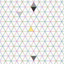
(a) The yellow triangle corresponds to the identity. From lightest to darkest gray the other colored elements are $x_{7}$, $\theta(1,2)s_{1}$, $s_{0}\theta(1,2)s_{1}$, and $\theta(1,2)$.

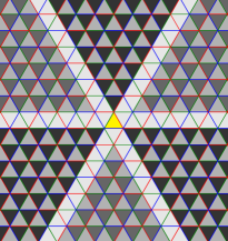
(b) From lightest to darkest gray: $X$, $\Theta_{1}$, $\Theta_{2}$, and $\Theta$.

Figure 1. Geometric realization of $W$ and the four regions.

Using the geometric realization of $W$ it is not hard to see that $W\setminus\{\operatorname{id}\}=X\uplus\Theta\uplus\Theta_{1}\uplus\Theta_{2}$, where $\uplus$ denotes a disjoint union, as is illustrated in Figure 1(b).

The geometric realization of $W$ allows us to describe certain lower intervals in an elegant way as the convex hull of a given set. We denote by $\operatorname{cen}(w)$ the centroid of $w\in W$. Let $W_{f}\coloneqq\langle s_{1},s_{2}\rangle\leq W$ (it is a dihedral group of order $6$). For $w$ in $W$, let $\mathcal{C}_{w}$ denote the convex hull of the set $\{\operatorname{cen}(yw)\,|\,y\in W_{f}\}$.

The following lemma appears in the proof of [LP20, Lemma 1.4].

Lemma 2.3.

Let $m$ and $n$ be non-negative integers. Then,

$$[\operatorname{id},\theta(m,n)]=\{w\in W\,|\,\operatorname{cen}(w)\in\mathcal{C}_{\theta(m,n)}\}.$$

For instance, the interval $[\operatorname{id},\theta(1,3)]$ is illustrated in Figure 2(a). We recall that $s_{1}$ and $s_{2}$ have been identified with the reflections through the lines that support the green and red sides of the identity triangle, respectively.

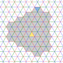
(a) Lower interval $[\operatorname{id},\theta(1,3)]$. The blue triangle corresponds to $\theta(1,3)$. The gray triangles correspond to the non-endpoints of $[\operatorname{id},\theta(1,3)]$.

(b) Lower interval $[\operatorname{id},\theta(1,3)s_{2}]$. The dark blue triangle corresponds to $\theta(1,3)s_{2}$. The dark gray triangles together with the dark blue triangle correspond to $\partial_{1,3}s_{2}$.

Figure 2. Geometric description of $[\operatorname{id},\theta(1,3)]$ and $[\operatorname{id},\theta(1,3)s_{2}]$.

Lemma 2.4.

Let $m$ and $n$ be non-negative integers. Set $s=s_{m,n}$. Then,

(2.8) $$[\operatorname{id},\theta(m,n)s]=[\operatorname{id},\theta(m,n)]\uplus\partial_{m,n}s,$$

where $\partial_{m,n}$ is the set formed by all the elements $x\in[\operatorname{id},\theta(m,n)]$ such that $x$ has a side belonging to the boundary of $[\operatorname{id},\theta(m,n)]$.

Proof.

It is clear that $[\operatorname{id},\theta(m,n)s]\supset[\operatorname{id},\theta(m,n)]\uplus\partial_{m,n}s$. For the other inclusion, we first notice that if $w\leq\theta(m,n)s$ then we either have $w\leq\theta(m,n)$ or $w=xs$ for $x\leq\theta(m,n)$. If $w\leq\theta(m,n)$ then there is nothing to prove. Thus we can assume $w\not\leq\theta(m,n)$. Therefore $w=xs$ for some $x\leq\theta(m,n)$. Since $x$ is inside and $w=xs$ is outside the interval $[\operatorname{id},\theta(m,n)]$, their shared ($s$-colored) side is in the boundary of $[\operatorname{id},\theta(m,n)]$. It follows that $x\in\partial_{m,n}$ and $w\in\partial_{m,n}s$.

In the proof of [LP20, Lemma 1.4], the authors showed that the boundary of the interval $[\operatorname{id},\theta(m,n)]$ is colored by $s$. This implies that for $x\in\partial_{m,n}$ the element $xs$ is outside the interval $[\operatorname{id},\theta(m,n)]$, so the union in Equation (2.8) is indeed disjoint. ∎

Lemma 2.4 is illustrated in Figure 2(b) for the pair $(m,n)=(1,3)$.

Remark 2.5.

For the more algebraic or combinatorially minded readers, we give an explicit description of the lower intervals without a proof. Although one can use these descriptions in some of the results that follow, we strongly prefer the geometric versions used in the paper.

For any pair of non-negative integers we define $a_{m,n}\coloneqq 2m+n$ and $b_{m,n}\coloneqq m+2n$. Let $f$ be the bijection of $\{0,1,2\}$ that fixes $0$ and permutes $1$ and $2$. The set

$$Y\coloneqq[\mbox{id},\theta(m,n)]\setminus\{\mbox{id}\}$$

is partitioned as follows (for all the sets below, we assume that $i\in\{0,1,2\}$):

(2.9) $$X\cap Y= \,\{\rho^{i}(x_{k})\,|\,1\leq k<a_{m,n}+3-i\}\uplus\{\rho^{i}(\sigma(x_{k}))\,|\,2\leq k<b_{m,n}+3-f(i)\}$$

(2.10) $$\Theta\cap Y= \,\{\rho^{i}(\theta(p,q))\,|\,a_{p,q}<a_{m,n}+1-i\mbox{ and }b_{p,q}<b_{m,n}+1-f(i)\}$$

(2.11) $$\Theta_{1}\cap Y= \,\{\rho^{i}(\theta(p,q)s_{p,q})\,|\,a_{p,q}<a_{m,n}-i\mbox{ and }b_{p,q}<b_{m,n}-f(i)\}\,\uplus$$

$$\,\{\rho^{i}(s_{0}\theta(p,q))\,|\,a_{p,q}<a_{m,n}-2+f(i)\mbox{ and }b_{p,q}<b_{m,n}-2+i\}$$

(2.12) $$\Theta_{2}\cap Y= \,\{\rho^{i}(s_{0}\theta(p,q)s_{p,q})\,|\,a_{p,q}<a_{m,n}-3+f(i)\mbox{ and }b_{p,q}<b_{m,n}-3+i\}$$

If one replaces every $<$ by $\leq$ in the description above, one obtains the set

$$[\mbox{id},\theta(m,n)s_{m,n}]\setminus\{\mbox{id}\}.$$

Lemma 2.6.

Let $m$ and $n$ be positive integers. Then, we have

(2.13) $$[\operatorname{id},\theta(m-1,n)]\cap[\operatorname{id},\theta(m,n-1)]=[\operatorname{id},\theta(m-1,n-1)s_{m-1,n-1}].$$

Proof.

This follows from Lemma 2.3 and Lemma 2.4, see Figure 3 for an illustration of this. ∎

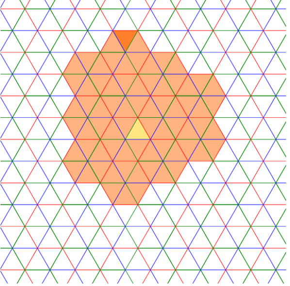
(a) The interval $[\operatorname{id},\theta(2,1)]$. The highlighted triangle corresponds to $\theta(2,1)$.

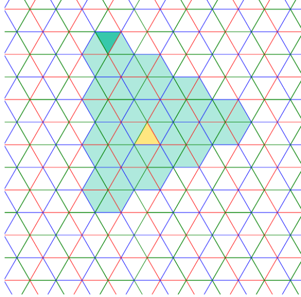
(b) The interval $[\operatorname{id},\theta(3,0)]$. The highlighted triangle corresponds to $\theta(3,0)$.

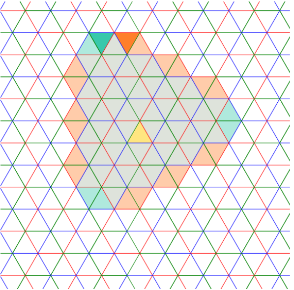
(c) The overlapping of Figure 3(a) and Figure 3(b). The triangles in the intersection are colored with gray.

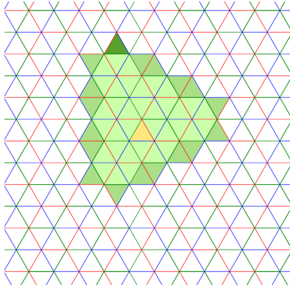
(d) The interval $[\operatorname{id},\theta(2,0)s_{1}]$. From lightest to darkest green: The interval $[\operatorname{id},\theta(2,0)]$, the set $\partial_{2,0}s_{1}\setminus\{\theta(2,0)s_{1}\}$ and the element $\theta(2,0)s_{1}$.

Figure 3. An example of Lemma 2.6 for the pair $(m,n)=(3,1)$.

2.2. The Hecke algebra of type $\tilde{A}_{2}$

The Hecke algebra $\mathcal{H}=\mathcal{H}(W)$ is the associative and unital $\mathbb{Z}[v,v^{-1}]$-algebra generated by $\mathbf{H}_{s_{0}}$, $\mathbf{H}_{s_{1}}$ and $\mathbf{H}_{s_{2}}$ subject to the relations

$$\mathbf{H}_{s_{i}}^{2}=(v^{-1}-v)\mathbf{H}_{s_{i}}+1,\quad \mbox{for }i\in\{0,1,2\},$$

$$\mathbf{H}_{s_{i}}\mathbf{H}_{s_{j}}\mathbf{H}_{s_{i}}=\mathbf{H}_{s_{j}}\mathbf{H}_{s_{i}}\mathbf{H}_{s_{j}},\quad \mbox{for }i\neq j.$$

Given $w\in W$ and a reduced expression $\underline{w}=r_{1}r_{2}\ldots r_{k}$ ($r_{i}\in S$, for all $i$) for $w$ we define $\mathbf{H}_{w}=\mathbf{H}_{r_{1}}\mathbf{H}_{r_{2}}\cdots\mathbf{H}_{r_{k}}$. It is well-known that $\mathbf{H}_{w}$ does not depend on the choice of the reduced expression. The set $\{\mathbf{H}_{w}\,|\,w\in W\}$ is a basis for $\mathcal{H}$ which is called the standard basis. Let $\underline{\mathbf{H}}_{s}=\mathbf{H}_{s}+v$. The right regular action of $\mathcal{H}$ is given by the formula

(2.14) $$\mathbf{H}_{x}\underline{\mathbf{H}}_{s}=\begin{cases}\mathbf{H}_{xs}+v\mathbf{H}_{x},&\text{if }xs>x;\\ \mathbf{H}_{xs}+v^{-1}\mathbf{H}_{x},&\text{if }xs<x.\end{cases}$$

In their seminal paper [KL79] Kazhdan and Lusztig introduced a new basis

$$\{\underline{\mathbf{H}}_{w}\,|\,w\in W\}$$

of $\mathcal{H}$ called the canonical basis, also known as the Kazhdan-Lusztig basis. We denote by $h_{x,w}(v)$ the corresponding Kazhdan-Lusztig polynomials defined by the equality

(2.15) $$\underline{\mathbf{H}}_{w}=\sum_{x\in W}h_{x,w}(v)\mathbf{H}_{x}.$$

We stress that in this section we use Soergel’s normalisation in [Soe97] rather than the standard $q$-notation used by Kazhdan and Lusztig in [KL79]. The passage from Kazhdan-Lusztig polynomials $P_{x,w}(q)$ in their $q$-version to Kazhdan-Lusztig polynomials $h_{x,w}(v)$ in their $v$-version is given by

(2.16) $$h_{x,w}(v)=v^{\ell(w)-\ell(x)}P_{x,w}(v^{-2}).$$

Henceforth, we use both versions of Kazhdan-Lusztig polynomials without further notice.

For additional background material and an algorithm to compute the canonical basis, we refer the reader to [Soe97, Section 2]. We conclude this section by recalling the formulas given in [LP20] for all the Kazhdan-Lusztig basis elements in $W$.

For $x\in W$, we define

$$\mathbf{N}_{x}\coloneqq\sum_{z\leq x}v^{\ell(x)-\ell(z)}\mathbf{H}_{z}.$$

Proposition 2.1.

[LP20, Proposition 1.6] The following formula holds

(2.17) $$\underline{\mathbf{H}}_{x_{n}}=\begin{cases}\mathbf{N}_{x_{n}},&\mbox{ if $n\leq 3$;}\\ \mathbf{N}_{x_{4}}+v\mathbf{N}_{x_{1}},&\mbox{ if $n=4$;}\\ \mathbf{N}_{x_{n}}+v\mathbf{N}_{x_{n-3}},&\mbox{ if }n\geq 5\mbox{ is odd;}\\ \mathbf{N}_{x_{n}}+v\mathbf{N}_{x_{n-3}}+v\mathbf{H}_{s_{1}s_{0}x_{n-5}}+v^{2}\mathbf{H}_{s_{0}x_{n-5}},&\mbox{ if }n\geq 5\mbox{ is even.}\\ \end{cases}$$

Proposition 2.2.

[LP20, Proposition 1.8] Let $m$ and $n$ be non-negative integers. We have

(2.18) $$\underline{\mathbf{H}}_{\theta(m,n)}=\sum_{i=0}^{\min(m,n)}v^{2i}\mathbf{N}_{\theta(m-i,n-i)}.$$

In particular, we have $\underline{\mathbf{H}}_{\theta(m,0)}=\mathbf{N}_{\theta(m,0)}$ and $\underline{\mathbf{H}}_{\theta(0,n)}=\mathbf{N}_{\theta(0,n)}$. Furthermore, if $s=s_{m,n}$ we have

(2.19) $$\underline{\mathbf{H}}_{s_{0}}\underline{\mathbf{H}}_{\theta(m,n)}=\underline{\mathbf{H}}_{s_{0}\theta(m,n)},\quad\underline{\mathbf{H}}_{\theta(m,n)}\underline{\mathbf{H}}_{s}=\underline{\mathbf{H}}_{\theta(m,n)s},$$

$$\mbox{ and }\quad\underline{\mathbf{H}}_{s_{0}}\underline{\mathbf{H}}_{\theta(m,n)}\underline{\mathbf{H}}_{s}=\underline{\mathbf{H}}_{s_{0}\theta(m,n)s}.$$

Proposition 2.1 and Proposition 2.2 are enough to compute all the Kazhdan-Lusztig basis elements in view of the first claim in the following lemma.

Lemma 2.3.

Suppose $\tau\in G$. Let $[x,y]$ be any Bruhat interval in $W$. Then,

• $P_{x,y}(q)=P_{\tau(x),\tau(y)}(q)$ (equivalently, $h_{x,y}(v)=h_{\tau(x),\tau(y)}(v)$).

• $[x,y]\simeq[\tau(x),\tau(y)]$ as posets.

Proof.

Both claims follow by the definition of Bruhat order and the definition of the Kazhdan-Lusztig polynomials. ∎

Lemma 2.3 tells us that if we prove the combinatorial invariance conjecture for a pair of intervals $[x,y]$ and $[x^{\prime},y^{\prime}]$ then the conjecture is immediately true for any pair of intervals of the form $[\tau(x),\tau(y)]$ and $[\tau^{\prime}(x^{\prime}),\tau^{\prime}(y^{\prime})]$, for all $\tau,\tau^{\prime}\in G$.

2.3. Trivial Kazhdan-Lusztig polynomials

For a Coxeter system $(W,S)$, define $T=\bigcup_{w\in W}wSw^{-1}$ to be the set of all reflections.

Definition 2.1.

Let $(W,S)$ be a Coxeter system. For $x\leq y$, we say that the interval $[x,y]$ satisfies property P if for every $z\in[x,y]$ we have

$$\left|\{t\in T:z<tz\leq y\}\right|=\ell(y)-\ell(z).$$

Thanks to the non-negativity theorem of the coefficients of the Kazhdan-Lusztig polynomials [EW14] we can restate [Car94, Theorem C] as follows.

Theorem 2.2.

For a Coxeter system $(W,S)$, and $x\leq y$, the following are equivalent:

1. $P_{x,y}(q)=1$.

2. $P_{z,w}(q)=1$ for all $z\in[x,y]$.

3. The interval $[x,y]$ satisfies property P.

Definition 2.3.

The Bruhat graph $\Omega_{W}([x,y])$ of $[x,y]$ is the directed graph defined as follows. The set of vertices is $[x,y]$ and the set of edges is

$$\{(w,tw):\mbox{ $w<tw$ and $t\in T$}\}.$$

The following is [Dye91, Proposition 3.3].

Proposition 2.4.

The Bruhat graph $\Omega_{W}([x,y])$ depends only on the poset type of the interval $[x,y]$.

Putting all the results of this section together we have the following proposition.

Proposition 2.5.

Let $(W,S)$ and $(W^{\prime},S^{\prime})$ be two Coxeter systems. Suppose $x,y\in W$ and $x^{\prime},y^{\prime}\in W^{\prime}$ are elements such that $[x,y]\cong[x^{\prime},y^{\prime}]$ as posets. If $P_{x,y}(q)=1$ then $P_{x^{\prime},y^{\prime}}(q)=1$.

Proof.

Suppose $P_{x,y}(q)=1$, by Theorem 2.2 we have $[x,y]$ satisfies the property P. By Proposition 2.4, Property P is a poset invariant, therefore $[x^{\prime},y^{\prime}]$ satisfies property P. By Theorem 2.2 we conclude $P_{x^{\prime},y^{\prime}}(q)=1$. ∎

2.4. Monotonicity and content

First, we recall the monotonicity of Kazhdan-Lusztig polynomials proved in [BM01] for affine Weyl groups and in [Pla17] for arbitrary Coxeter systems.

Proposition 2.1.

If $x\leq z\leq y$ then

(2.20) $$h_{x,y}(v)-v^{\ell(z)-\ell(x)}h_{z,y}(v)\in\mathbb{N}[v].$$

Equivalently,

(2.21) $$P_{x,y}(q)-P_{z,y}(q)\in\mathbb{N}[q].$$

Definition 2.2.

Given $h_{1}(v),h_{2}(v)\in\mathbb{Z}[v,v^{-1}]$, we write $h_{1}(v)\geq h_{2}(v)$ if $h_{1}(v)-h_{2}(v)\in\mathbb{N}[v,v^{-1}]$. Given $x\in W$ and $H\in\mathcal{H}$, we define $G_{x}(H)$ to be the coefficient of $\mathbf{H}_{x}$ when we expand $H$ in terms of the standard basis of $\mathcal{H}$. We say an element $H\in\mathcal{H}$ is monotonic if

$$G_{y}(H)\geq v^{\ell(x)-\ell(y)}G_{x}(H),$$

for all $y\leq x$. Finally, we write $H_{1}\geq_{\mathbf{H}}H_{2}$ if $G_{x}(H_{1}-H_{2})\in\mathbb{N}[v,v^{-1}]$, for all $x\in W$.

An obvious example of a monotonic element is $\mathbf{N}_{w}$. Also, by (2.20) we know that the canonical basis elements $\underline{\mathbf{H}}_{w}$ are monotonic in an arbitrary Coxeter system. On the other hand, it is easy to see that the sum of two monotonic elements is monotonic. The following (a weaker version of [BBP21, Lemma 3.3]) is another way to produce new monotonic elements from old ones.

Lemma 2.3.

For $s\in S$, if $H\in\mathcal{H}$ is monotonic, then $H\underline{\mathbf{H}}_{s}$ is also monotonic.

Definition 2.4.

Let $H\in\mathcal{H}$. We define the content of $H$ as

(2.22) $$c(H)=\sum_{x\in W}G_{x}(H)(1)\in\mathbb{Z}.$$

For instance, the content of $\mathbf{N}_{w}$ is equal to the number of elements in the lower Bruhat interval $[\operatorname{id},w]$. For $s=s_{m,n}$ we have the following formulas

(2.23) $$c(\mathbf{N}_{\theta(m,n)}) =\left|[\operatorname{id},\theta(m,n)]\right|=3m^{2}+3n^{2}+12mn+9m+9n+6.$$

(2.24) $$c(\mathbf{N}_{\theta(m,n)s}) =\left|[\operatorname{id},\theta(m,n)s]\right|=3m^{2}+3n^{2}+12mn+15m+15n+12.$$

(2.25) $$c(\mathbf{N}_{s_{0}\theta(m,n)s}) =\left|[\operatorname{id},s_{0}\theta(m,n)s]\right|=3m^{2}+3n^{2}+12mn+21m+21n+22.$$

The formula in (2.23) is already in [LP20, Lemma 1.4]. The remaining formulas can be obtained in a similar way, using the geometric realization of $W$ as in Figure 1(b). Using (2.14) one can easily prove the following lemma.

Lemma 2.5.

For any $H\in\mathcal{H}$ and $s\in S$ we have $c(H\underline{\mathbf{H}}_{s})=2c(H).$

Remark 2.6.

We can use the order $\geq_{\mathbf{H}}$ and the content to show an equality in $\mathcal{H}$. More precisely, let $H_{1},H_{2}\in\mathcal{H}$. If $H_{1}\geq_{\mathbf{H}}H_{2}$ and $c(H_{1})=c(H_{2})$ then $H_{1}=H_{2}$.

3. New formulas for Kazhdan-Lusztig basis elements

Although Proposition 2.2 is enough to compute all of the Kazhdan-Lusztig basis elements corresponding to elements in sets $\Theta_{1}$ and $\Theta_{2}$, we want more explicit formulas that allow us to compute the Kazhdan-Lusztig polynomials in a more direct way. This is the content of Proposition 3.1 and Proposition 3.3 below. In this section we use the convention that $\underline{\mathbf{H}}_{\theta(m,n)}$ and $\mathbf{N}_{\theta(m,n)}$ are zero if $m$ or $n$ are negative.

Proposition 3.1.

Let $m$ and $n$ be non-negative integers and $s=s_{m,n}$. We have

(3.1) $$\underline{\mathbf{H}}_{\theta(m,n)s}=\mathbf{N}_{\theta(m,n)s}+v\underline{\mathbf{H}}_{\theta(m-1,n)}+v\underline{\mathbf{H}}_{\theta(m,n-1).}$$

Proof.

The $m=n=0$ case is easily checked by hand.
Suppose that $m>0$ and $n=0$ (the case $m=0$ and $n>0$ is similar). By Proposition 2.2 we have $\underline{\mathbf{H}}_{\theta(m,0)}=\mathbf{N}_{\theta(m,0)}$. Therefore, Equation (2.19) implies $\underline{\mathbf{H}}_{\theta(m,0)s}=\mathbf{N}_{\theta(m,0)}\underline{\mathbf{H}}_{s}$. Therefore, this case is reduced to check the identity

(3.2) $$\mathbf{N}_{\theta(m,0)}\underline{\mathbf{H}}_{s}=\mathbf{N}_{\theta(m,0)s}+v\mathbf{N}_{\theta(m-1,0)}.$$

To prove this we use Remark 2.6. Let

$$H_{1}=\mathbf{N}_{\theta(m,0)}\underline{\mathbf{H}}_{s}\mbox{ and }H_{2}=\mathbf{N}_{\theta(m,0)s}+v\mathbf{N}_{\theta(m-1,0)}.$$

By Lemma 2.5, Equation (2.23) and Equation (2.24) we obtain

(3.3) $$c(H_{1})=c(H_{2})=2(3m^{2}+9m+6).$$

We have

(3.4) $$G_{x}(H_{2})=\begin{cases}v^{\ell(\theta(m,0)s)-\ell(x)},&\mbox{if }x\leq\theta(m,0)s\mbox{ and }x\not\leq\theta(m-1,0);\\ v^{\ell(\theta(m,0)s)-\ell(x)}+v^{\ell(\theta(m-1,0))+1-\ell(x)},&\mbox{if }x\leq\theta(m-1,0);\\ 0,&\mbox{otherwise.}\end{cases}$$

On the other hand, by Equation (2.14) we get

(3.5) $$G_{\theta(m,0)s}(H_{1})=1\quad\mbox{ and }\quad G_{\theta(m-1,0)}(H_{1})=v^{3}+v.$$

By Lemma 2.3 $H_{1}$ is monotonic. Therefore, (3.5) implies

(3.6) $$G_{x}(H_{1})\geq\begin{cases}v^{\ell(\theta(m,0)s)-\ell(x)},&\mbox{if }x\leq\theta(m,0)s\mbox{ and }x\not\leq\theta(m-1,0);\\ v^{\ell(\theta(m,0)s)-\ell(x)}+v^{\ell(\theta(m-1,0))+1-\ell(x)},&\mbox{if }x\leq\theta(m-1,0).\end{cases}$$

In the lower part of (3.6) we are using that $\ell(\theta(m-1,0))+3=\ell(\theta(m,0)s)$. By combining (3.4) and (3.6) we obtain $H_{1}\geq_{\mathbf{H}}H_{2}$, thus proving the lemma in this case.

We now assume that $m,n>0$. By (2.18) we have

(3.7) $$\underline{\mathbf{H}}_{\theta(m,n)}=\mathbf{N}_{\theta(m,n)}+v^{2}\underline{\mathbf{H}}_{\theta(m-1,n-1)}.$$

Multiplying on the right by $\underline{\mathbf{H}}_{s}$ (note that $s=s_{m,n}=s_{m-1,n-1}$) and assuming by induction that (3.1) holds for $\theta(m-1,n-1)$ we obtain that

$$\underline{\mathbf{H}}_{\theta(m,n)s} =\mathbf{N}_{\theta(m,n)}\underline{\mathbf{H}}_{s}+v^{2}\underline{\mathbf{H}}_{\theta(m-1,n-1)}\underline{\mathbf{H}}_{s}$$

$$=\mathbf{N}_{\theta(m,n)}\underline{\mathbf{H}}_{s}+v^{2}\underline{\mathbf{H}}_{\theta(m-1,n-1)s}$$

$$=\mathbf{N}_{\theta(m,n)}\underline{\mathbf{H}}_{s}+v^{2}\mathbf{N}_{\theta(m-1,n-1)s}+v^{3}\underline{\mathbf{H}}_{\theta(m-2,n-1)}+v^{3}\underline{\mathbf{H}}_{\theta(m-1,n-2)}.$$

Therefore, using (3.7) twice, our claim reduces to prove the following identity

(3.8) $$\mathbf{N}_{\theta(m,n)}\underline{\mathbf{H}}_{s}+v^{2}\mathbf{N}_{\theta(m-1,n-1)s}=\mathbf{N}_{\theta(m,n)s}+v\mathbf{N}_{\theta(m-1,n)}+v\mathbf{N}_{\theta(m,n-1)}.$$

As before, we use Remark 2.6. Let $L$ and $R$ be the left-hand side and the right-hand side of (3.8), respectively. A combination of (2.23), (2.24), and Lemma 2.5 yields

(3.9) $$c(L)=c(R)=3(3m^{2}+3n^{2}+12mn+5m+5n+4).$$

It remains to show that $L\geq_{\mathbf{H}}R$. Set $a_{0}=\theta(m,n)s$, $a_{1}=\theta(m-1,n)$, $a_{2}=\theta(m,n-1)$, and $a_{3}=\theta(m-1,n-1)s$. By the definition of $R$ and Lemma 2.6 we get

(3.10) $$G_{x}(R)=\begin{cases}v^{\ell(a_{0})-\ell(x)},&\mbox{if }x\leq a_{0},\,x\not\leq a_{1},\mbox{ and }x\not\leq a_{2};\\ v^{\ell(a_{0})-\ell(x)}+v^{\ell(a_{1})+1-\ell(x)},&\mbox{if }x\leq a_{1}\mbox{ and }x\not\leq a_{2};\\ v^{\ell(a_{0})-\ell(x)}+v^{\ell(a_{2})+1-\ell(x)},&\mbox{if }x\not\leq a_{1}\mbox{ and }x\leq a_{2};\\ v^{\ell(a_{0})-\ell(x)}+2v^{\ell(a_{2})+1-\ell(x)},&\mbox{if }x\leq a_{3};\\ 0,&\mbox{otherwise.}\end{cases}$$

We have used that $\ell(a_{1})=\ell(a_{2})$. By the definition of $L$ and Equation (2.14) we get

(3.11) $$G_{a_{0}}(L) =1;$$

(3.12) $$G_{a_{1}}(L) =v^{3}+v;$$

(3.13) $$G_{a_{2}}(L) =v^{3}+v;$$

(3.14) $$G_{a_{3}}(L) =v^{4}+2v^{2}.$$

Using Lemma 2.3 and the fact that the sum of two monotonic elements is monotonic we conclude that $L$ is monotonic as well. It follows that

(3.15) $$G_{x}(L)\geq\begin{cases}v^{\ell(a_{0})-\ell(x)},&\mbox{if }x\leq a_{0},\,x\not\leq a_{1},\mbox{ and }x\not\leq a_{2};\\ v^{\ell(a_{0})-\ell(x)}+v^{\ell(a_{1})+1-\ell(x)},&\mbox{if }x\leq a_{1}\mbox{ and }x\not\leq a_{2};\\ v^{\ell(a_{0})-\ell(x)}+v^{\ell(a_{2})+1-\ell(x)},&\mbox{if }x\not\leq a_{1}\mbox{ and }x\leq a_{2};\\ v^{\ell(a_{0})-\ell(x)}+2v^{\ell(a_{2})+1-\ell(x)},&\mbox{if }x\leq a_{3},\end{cases}$$

Where we have used the following equalities.

(3.16) $$\ell(a_{1})+3 =\ell(a_{0}),$$

(3.17) $$\ell(a_{2})+3 =\ell(a_{0}),$$

(3.18) $$\ell(a_{3})+4 =\ell(a_{0}).$$

By combining (3.10) and (3.15) we obtain $L\geq_{\mathbf{H}}R$, as we wanted to show. ∎

The formula for $\underline{\mathbf{H}}_{s_{0}\theta(m,n)s_{m,n}}$ is more involved. To describe this formula we need to consider the following element. For $x,y\in W$, we define

(3.19) $$\mathbf{M}_{x,y}\coloneqq\sum_{w\leq x\mbox{ or }w\leq y}v^{\ell(x)-\ell(w)}\mathbf{H}_{w}.$$

Remark 3.2.

One has the equality $\mathbf{M}_{x,y}=\mathbf{M}_{y,x}$ if and only if $\ell(x)=\ell(y)$.

The content of $\mathbf{M}_{x,y}$ equals the number of elements in the union of the lower intervals $[\operatorname{id},x]$ and $[\operatorname{id},y]$. In particular, for any pair $(m,n)$ of positive integers we have

(3.20) $$c(\mathbf{M}_{\rho(\theta(m,n-1))s,\rho^{2}(\theta(m-1,n))s})=3m^{2}+3n^{2}+12mn+9m+9n+2,$$

where $s=s_{m,n}$. Note that $s$ is such that $\rho(\theta(m,n-1))s>\rho(\theta(m,n-1))$ and $\rho^{2}(\theta(m-1,n))s>\rho^{2}(\theta(m-1,n))$.

Proposition 3.3.

Let $m$ and $n$ be non-negative integers and $s=s_{m,n}$.

If $m=n=0$ then

(3.21) $$\underline{\mathbf{H}}_{s_{0}\theta(0,0)s}=\mathbf{N}_{s_{0}\theta(0,0)s}+v^{2}\mathbf{N}_{s_{0}}.$$

If $m>0$ and $n=0$ then

(3.22) $$\underline{\mathbf{H}}_{s_{0}\theta(m,0)s} =\mathbf{N}_{s_{0}\theta(m,0)s}+v\mathbf{M}_{s_{0}\theta(m-1,0),\rho(\theta(m-1,0))}+v\underline{\mathbf{H}}_{\rho^{2}(\theta(m-1,0))s},$$

(3.23) $$=\mathbf{N}_{s_{0}\theta(m,0)s}+v\mathbf{M}_{\rho^{2}(\theta(m-1,0))s,\rho(\theta(m-1,0))}+v\underline{\mathbf{H}}_{s_{0}\theta(m-1,0)}.$$

If $m=0$ and $n>0$ then

(3.24) $$\underline{\mathbf{H}}_{s_{0}\theta(0,n)s} =\mathbf{N}_{s_{0}\theta(0,n)s}+v\mathbf{M}_{s_{0}\theta(0,n-1),\rho^{2}(\theta(0,n-1))}+v\underline{\mathbf{H}}_{\rho(\theta(0,n-1))s},$$

(3.25) $$=\mathbf{N}_{s_{0}\theta(0,n)s}+v\mathbf{M}_{\rho(\theta(0,n-1))s,\rho^{2}(\theta(0,n-1))}+v\underline{\mathbf{H}}_{s_{0}\theta(0,n-1)}.$$

If $m>0$ and $n>0$ then

(3.26) $$\underline{\mathbf{H}}_{s_{0}\theta(m,n)s} =\mathbf{N}_{s_{0}\theta(m,n)s}+v\mathbf{M}_{s_{0}\theta(m,n-1),s_{0}\theta(m-1,n)}+v\underline{\mathbf{H}}_{\rho(\theta(m,n-1))s}+v\underline{\mathbf{H}}_{\rho^{2}(\theta(m-1,n))s},$$

(3.27) $$=\mathbf{N}_{s_{0}\theta(m,n)s}+v\mathbf{M}_{\rho(\theta(m,n-1))s,\rho^{2}(\theta(m-1,n))s}+v\underline{\mathbf{H}}_{s_{0}\theta(m,n-1)}+v\underline{\mathbf{H}}_{s_{0}\theta(m-1,n)}.$$

Proof.

We only prove the case $m>0$ and $n>0$, the proof of the remaining cases being analogous.

Multiplying (3.1) by $\underline{\mathbf{H}}_{s_{0}}$ on the left and using (2.19) we obtain

(3.28) $$\underline{\mathbf{H}}_{s_{0}\theta(m,n)s}=\underline{\mathbf{H}}_{s_{0}}\mathbf{N}_{\theta(m,n)s}+v\underline{\mathbf{H}}_{s_{0}\theta(m-1,n)}+v\underline{\mathbf{H}}_{s_{0}\theta(m,n-1)}.$$

Therefore, the proof of (3.27) reduces to show the identity

(3.29) $$\underline{\mathbf{H}}_{s_{0}}\mathbf{N}_{\theta(m,n)s}=\mathbf{N}_{s_{0}\theta(m,n)s}+v\mathbf{M}_{\rho(\theta(m,n-1))s,\rho^{2}(\theta(m-1,n))s}.$$

To prove this we use Remark 2.6. Let $L$ and $R$ be the left-hand side and the right-hand side of (3.29), respectively. By (2.24), (2.25), (3.20), and (the left version of) Lemma 2.5 we get

$$c(L)=c(R)=6m^{2}+6n^{2}+24mn+30m+30n+24.$$

It remains to show that $L\geq_{\mathbf{H}}R$. Set $a_{0}=s_{0}\theta(m,n)s$, $a_{1}=\rho(\theta(m,n-1))s$, and $a_{2}=\rho^{2}(\theta(m-1,n))s$. By the definition of $R$ we get

(3.30) $$G_{x}(R)=\begin{cases}v^{\ell(a_{0})-\ell(x)},&\mbox{if }x\leq a_{0},\,x\not\leq a_{1}\mbox{ and }x\not\leq a_{2};\\ v^{\ell(a_{0})-\ell(x)}+v^{\ell(a_{1})-\ell(x)+1},&\mbox{if }x\leq a_{1}\mbox{ or }x\leq a_{2};\\ 0,&\mbox{otherwise.}\end{cases}$$

In the second line, we have used that $\ell(a_{1})=\ell(a_{2})$. We notice that $s_{0}a_{1}<a_{1}$ and $s_{0}a_{2}<a_{2}$. Then, the left version of Equation (2.14) yields $G_{a_{0}}(L)=1$ and $G_{a_{1}}(L)=G_{a_{2}}(L)=v^{3}+v$.

By Lemma 2.3 $L$ is monotonic. It follows that

(3.31) $$G_{x}(L)\geq\begin{cases}v^{\ell(a_{0})-\ell(x)},&\mbox{if }x\leq a_{0},\,x\not\leq a_{1},\mbox{ and }x\not\leq a_{2};\\ v^{\ell(a_{0})-\ell(x)}+v^{\ell(a_{1})-\ell(x)+1},&\mbox{if }x\leq a_{1}\mbox{ or }x\leq a_{2}.\end{cases}$$

Where we have used that $G_{a_{1}}(L)=G_{a_{2}}(L)$, and the fact that $\ell(a_{0})=\ell(a_{1})+3$. By combining (3.30) and (3.31) we obtain $L\geq_{\mathbf{H}}R$. This finishes the proof of (3.27).

Finally, (3.26) is obtained from (3.27) by inverting and then applying a power of $\rho$. Indeed, we have the following identity in $W$:

(3.32) $$\left[\rho^{j}(\theta(m,n))\right]^{-1}=\rho^{j+n-m}(\theta(n,m)).$$

Using this identity to invert all the elements of $W$ occurring in (3.27) we get

(3.33) $$\underline{\mathbf{H}}_{s\rho^{k}(\theta(n,m))s_{0}}= \mathbf{N}_{s\rho^{k}(\theta(n,m))s_{0}}+v\mathbf{M}_{s\rho^{k}(\theta(n-1,m)),s\rho^{k}(\theta(n,m-1))}+$$

$$v\underline{\mathbf{H}}_{\rho^{k-1}(\theta(n-1,m))s_{0}}+v\underline{\mathbf{H}}_{\rho^{k+1}(\theta(n,m-1))s_{0}},$$

where $k=n-m$. Then, we act by $\rho^{-k}$ on the equality above, and using the fact that $\rho^{-k}(s)=s_{0}$ and $\rho^{-k}(s_{0})=s_{n,m}\eqqcolon\tilde{s}$, we obtain

$$\underline{\mathbf{H}}_{s_{0}\theta(n,m)\tilde{s}}=\mathbf{N}_{s_{0}\theta(n,m)\tilde{s}}+v\mathbf{M}_{s_{0}\theta(n,m-1),s_{0}\theta(n-1,m)}+v\underline{\mathbf{H}}_{\rho^{2}(\theta(n-1,m))\tilde{s}}+v\underline{\mathbf{H}}_{\rho(\theta(n,m-1))\tilde{s}}.$$

Since $\ell(s_{0}\theta(n,m-1))=\ell(s_{0}\theta(n-1,m))$, by Remark 3.2 we get

$$\underline{\mathbf{H}}_{s_{0}\theta(n,m)\tilde{s}}=\mathbf{N}_{s_{0}\theta(n,m)\tilde{s}}+v\mathbf{M}_{s_{0}\theta(n-1,m),s_{0}\theta(n,m-1)}+v\underline{\mathbf{H}}_{\rho^{2}(\theta(n-1,m))\tilde{s}}+v\underline{\mathbf{H}}_{\rho(\theta(n,m-1))\tilde{s}}.$$

This last equality is (3.26) with the roles of $m$ and $n$ switched. ∎

4. Two poset invariants

For the proof of the main result of this paper it will be useful to have at hand certain invariants that will allow us to easily discard the occurrence of certain poset isomorphisms.

4.1. $m$-joins

Definition 4.1.

Let $[x,y]$ be an interval and $m$ be a positive integer. Let $a,b\in[x,y]$ be such that $\ell(a)=\ell(b)$. We say that an element $z\in[x,y]$ is an $m$-join of $a$ and $b$ if $a\leq z$, $b\leq z$, and $\ell(z)=\ell(a)+m=\ell(b)+m$. We denote by $\mathcal{J}_{a,b}^{[x,y]}(m)$ the set of all $m$-joins of $a$ and $b$ in the interval $[x,y]$.

Remark 4.2.

It is worth mentioning the fact that $1$-joins have already been relevant for the combinatorial invariance conjecture. As a matter of fact, it was proved in [BCM06, Theorem 3.2] that for $a\neq b$ we have

(4.1) $$\left|\mathcal{J}_{a,b}^{[x,y]}(1)\right|\leq 2$$

in any Coxeter system. Although we will not use this result in our proof, it is interesting to notice the similarity between (4.1) and our Lemma 4.4.

The following result is immediate from the definitions.

Lemma 4.3.

Let $\phi\colon[x,y]\longrightarrow[x^{\prime},y^{\prime}]$ be an isomorphism of posets. Suppose $a,b\in[x,y]$ are such that $\ell(a)=\ell(b)$. Then, $\phi(\mathcal{J}_{a,b}^{[x,y]}(m))=\mathcal{J}_{\phi(a),\phi(b)}^{[x^{\prime},y^{\prime}]}(m)$, for all $m$. In particular, $\mathcal{J}_{a,b}^{[x,y]}(m)$ and $\mathcal{J}_{\phi(a),\phi(b)}^{[x^{\prime},y^{\prime}]}(m)$ have the same number of elements.

As we have seen in Proposition 3.3, there are certain key elements in $W$ that allow us to compute the canonical basis elements in a simple way, namely those indexing the $\mathbf{M}$ and $\underline{\mathbf{H}}$ elements appearing in the formulas in Proposition 3.3. In the following lemma, we will explore the number of $2$-joins of some of these elements. These numbers are going to be important poset invariants to be used in our proof of the conjecture.

Lemma 4.4.

Let $[x,y]$ be an interval such that $y=s_{0}\theta(m,n)s,$ where $s=s_{m,n}$. When they make sense, we define

(4.2) $$z_{1} \coloneqq s_{0}\theta(m,n-1); z_{2} \coloneqq s_{0}\theta(m-1,n);$$

(4.3) $$z_{3} \coloneqq\rho^{2}(\theta(m-1,n))s; z_{4} \coloneqq\rho(\theta(m,n-1))s.$$

We remark that $z_{1}$ and $z_{4}$ (resp. $z_{2}$ and $z_{3}$) are only defined if $n>0$ (resp. $m>0$). Suppose $i$ and $j$ are such that both $z_{i}$ and $z_{j}$ are defined and belong to $[x,y]$ with $i\neq j$. We have

$$\left|\mathcal{J}_{z_{i},z_{j}}^{[x,y]}(2)\right|=\begin{cases}3,&\mbox{ if $\{i,j\}=\{1,2\}$ or $\{i,j\}=\{3,4\}$;}\\ 2,&\mbox{ otherwise}.\end{cases}$$

Proof.

We only prove the case where $m>0$ and $n>0$. This is when the four elements $z_{1}$, $z_{2}$, $z_{3}$, and $z_{4}$ are defined. The remaining cases ($m=0$ and $n>0$, or $m>0$ and $n=0$) are similar and easier.

We notice that $\ell(z_{i})=\ell(y)-3$ for $i\in\{1,2,3,4\}$. Therefore,

(4.4) $$\mathcal{J}_{z_{i},z_{j}}^{[x,y]}(2)=\{w\in C_{y}\,|\,z_{i}<w\mbox{ and }z_{j}<w\}.$$

We recall that the set $C_{y}$ is given in Lemma 2.2. See Figure 4 for a picture of the elements of $C_{y}$ and the $z_{i}$’s. The elements of $C_{y}$ relate with the $z_{i}$’s in the following way:

(4.5) $$z_{3},z_{4} <\theta(m,n)s;$$

(4.6) $$z_{2},z_{3},z_{4} <\rho(\theta(m-1,n+1))s;$$

(4.7) $$z_{1},z_{2},z_{3} <s_{0}\theta(m-1,n+1);$$

(4.8) $$z_{1},z_{3},z_{4} <\rho^{2}(\theta(m+1,n-1))s;$$

(4.9) $$z_{1},z_{2},z_{4} <s_{0}\theta(m+1,n-1);$$

(4.10) $$z_{1},z_{2} <s_{0}\theta(m,n).$$

The lemma follows by combining (4.4) and (4.8). For instance,

(4.11) $$\mathcal{J}_{z_{1},z_{2}}^{[x,y]}(2)=\{s_{0}\theta(m-1,n+1),s_{0}\theta(m+1,n-1),s_{0}\theta(m,n)\}$$

since $s_{0}\theta(m-1,n+1)$, $s_{0}\theta(m+1,n-1)$ and $s_{0}\theta(m,n)$ are the only $3$ elements of $C_{y}$ which are simultaneously greater than $z_{1}$ and $z_{2}$. ∎

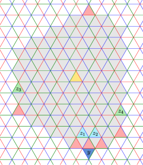
Figure 4. The triangles corresponding to the elements of the set $C_{y}$ for $y=s_{0}\theta(1,3)s_{2}$ are colored in pink. For reference, we colored all alcoves inside the interval $[\operatorname{id},y]$. As before, the yellow triangle corresponds to the identity in $W$.

4.2. Z-invariants

The following result [BB05, Exercises 5.7 and 5.8] is fundamental for our proof, as explained in the introduction.

Proposition 4.1.

If $[x,y]\sim[x^{\prime},y^{\prime}]$ and $\ell(y)-\ell(x)\leq 4$ then $P_{x,y}(q)=P_{x^{\prime},y^{\prime}}(q)$.

Before embarking in the proof, we need to define the key poset invariant.

Definition 4.2.

Let $[x,y]$ be any interval. For any integer $m\geq 3$ we define

(4.12) $$Z_{x,y}^{m}=\{z\in[x,y]\,|\,\ell(y)-\ell(z)=m\mbox{ and }P_{z,y}(q)=1+q\}.$$

Lemma 4.3.

Let $\phi\colon[x,y]\longrightarrow[x^{\prime},y^{\prime}]$ be a poset isomorphism. If $1\leq m\leq 4$, then $\phi(Z_{x,y}^{m})=Z_{x^{\prime},y^{\prime}}^{m}$. In particular, $|Z_{x,y}^{m}|=|Z_{x^{\prime},y^{\prime}}^{m}|$.

Proof.

This is a direct consequence of Proposition 4.1. ∎

The following lemmas show the power of the Z-invariant.

Lemma 4.4.

Let $[x,y]$ be an interval with $y\in\Theta_{1}\cup\Theta_{2}\cup X$. If $|Z_{x,y}^{3}|=1$ then $P_{x,y}(q)=1+q$.

Proof.

We need to split the proof in three cases: $y\in\Theta_{1}$, $y\in\Theta_{2}$, or $y\in X$.

Let us first assume that $y\in\Theta_{1}$. We can assume that $y=\theta(m,n)s_{m,n}$ for some $m,n\in\mathbb{N}$. By Proposition 3.1 we have $Z_{x,y}^{3}=\{\theta(m-1,n)\}$ or $Z_{x,y}^{3}=\{\theta(m,n-1)\}$. Suppose we are in the former case (the latter is treated similarly and is going to be omitted). Then $m>0$ and $\theta(m-1,n)\in[x,y]$, and $\theta(m,n-1)\notin[x,y]$ (if $\theta(m,n-1)\in[x,y]$ then we would have $\theta(m,n-1)\in Z^{3}_{x,y}$, and therefore $|Z^{3}_{x,y}|=2$, contradicting our hypothesis).
Suppose that $P_{x,y}(q)\neq 1+q$. An inspection of (2.18) and (3.1) reveals that $m>1$, $n>0$ and $\theta(m-2,n-1)\in[x,y]$. In particular, we have $x\leq\theta(m-2,n-1)$. Since $\theta(m-2,n-1)<\theta(m,n-1)$ we conclude that $\theta(m,n-1)\in[x,y]$ contradicting our conclusion in the last paragraph. Thus, $P_{x,y}(q)=1+q$, proving the lemma in this case.

Suppose now that $y\in\Theta_{2}$. We can assume that $y=s_{0}\theta(m,n)s_{m,n}$. The result follows by a case-by-case inspection of the formulas given in Proposition 3.3. Indeed, if $m=n=0$ then $Z_{x,y}^{3}=\emptyset$ and there is nothing to prove. Suppose now that $m>0$ and $n=0$. By (3.22) or (3.23) we have $Z_{x,y}^{3}=\{s_{0}\theta(m-1,0)\}$ or $Z_{x,y}^{3}=\{\rho^{2}(\theta(m-1,0))s_{m,n}\}$. If $Z_{x,y}^{3}=\{s_{0}\theta(m-1,0)\}$ (resp. $Z_{x,y}^{3}=\{\rho^{2}(\theta(m-1,0))s_{m,n}\}$) then we use (3.22) (resp. (3.23)) to conclude that $P_{x,y}(q)=1+q$. The case $m=0$ and $n>0$ is treated similarly.
We can now assume that $m>0$ and $n>0$. By (3.26) or (3.27) we have that $Z_{x,y}^{3}=\{z_{i}\}$, for some $1\leq i\leq 4$ and where $z_{i}$ is as in Lemma 4.4. If $Z_{x,y}^{3}=\{z_{1}\}$ or $Z_{x,y}^{3}=\{z_{2}\}$ (resp. $Z_{x,y}^{3}=\{z_{3}\}$ or $Z_{x,y}^{3}=\{z_{4}\}$) then we use (3.26) (resp. (3.27)) to conclude that $P_{x,y}(q)=1+q$, as we wanted to show.

Finally, we suppose $y\in X$. Without loss of generality, $y=x_{k}$. Furthermore, we assume that $k$ is even and greater than or equal to $6$, since the other cases are easier. We prove something stronger, namely that if $Z_{x,y}^{3}\neq\emptyset$ then $P_{x,y}(q)=1+q$. To see this we first notice that $x_{k-3}$ and $s_{1}s_{0}x_{k-5}$ (resp. $s_{0}x_{k-5}$) are incomparable in the Bruhat order. Furthermore, a direct computation reveals that if $x<s_{1}s_{0}x_{k-5}$ and $x\neq s_{0}x_{k-5},$ then $x\leq x_{k-3}$. On the other hand, by Equation (2.17) if $Z_{x,y}^{3}\neq\emptyset$ then we have that either $x\leq x_{k-3}$ or $x\leq s_{1}s_{0}x_{k-5}$. We must have one and only one of the following possibilities: $x\leq x_{k-3}$, $x=s_{1}s_{0}x_{k-5}$ or $x=s_{0}x_{k-5}$. An inspection of the formulas in Equation (2.17) shows that in any of these three cases we have $P_{x,y}(q)=1+q$. ∎

Remark 4.5.

The argument given in the final case of the proof of Lemma 4.4 shows that if $y\in X$ and $x\leq y$ we have

(4.13) $$P_{x,y}(q)=\begin{cases}1,&\mbox{if }Z_{x,y}^{3}=\emptyset;\\ 1+q,&\mbox{if }Z_{x,y}^{3}\neq\emptyset.\end{cases}$$

Lemma 4.6.

Let $[x,y]$ be an interval with $y\in\Theta_{1}\cup X$. If $Z^{3}_{x,y}=\emptyset$ then $P_{x,y}(q)=1$.

Proof.

The claim follows by an inspection of the formulas in Proposition 2.1 and Proposition 3.1. ∎

Lemma 4.7.

Let $[x,y]$ be an interval with $y\in\Theta_{2}$. Suppose that $Z_{x,y}^{3}=\emptyset$. If $P_{x,y}(q)\neq 1$ then the following three conditions hold:

1. $P_{x,y}(q)=1+q$;

2. $|Z_{x,y}^{4}|=1$;

3. $\ell(y)-\ell(x)=4$ or $\ell(y)-\ell(x)=5$.

Proof.

We can assume that $y=s_{0}\theta(m,n)s_{m,n}$ for some non-negative integers $m$ and $n$. We first notice that if $m$ and $n$ are positive then by looking at (3.26) or (3.27) we get $P_{x,y}(q)=1$, since otherwise $Z_{x,y}^{3}\neq\emptyset$. It follows that $m=0$ or $n=0$. We will prove that one of the following six cases occur:

(4.14) $$\begin{array}[]{l}m=0,\,n=0,\mbox{ and }x=s_{0};\\ m=0,\,n=0,\mbox{ and }x=\operatorname{id};\\ m>0,\,n=0,\mbox{ and }x=\rho(\theta(m-1,0));\\ m>0,\,n=0,\mbox{ and }x=\rho(x_{2m});\\ m=0,\,n>0,\mbox{ and }x=\rho^{2}(\theta(0,n-1));\\ m=0,\,n>0,\mbox{ and }x=\rho^{2}(\sigma(x_{2n})).\end{array}$$

If $m=n=0$ then (3.21) yields the first two cases in (4.14). Let us now assume that $m>0$ and $n=0$. In this case we look at (3.22) or (3.23) in order to conclude that the elements $x\leq y$ such that $Z_{x,y}^{3}=\emptyset$ and $P_{x,y}(q)\neq 1$ are those satisfying

(4.15) $$\qquad x\not\leq s_{0}\theta(m-1,0),\qquad x\not\leq\rho^{2}(\theta(m-1,0))s_{m,0},\quad\mbox{ and }\qquad x\leq\rho(\theta(m-1,0)).$$

A direct computation shows that the only elements satisfying (4.15) are $\rho(\theta(m-1,0))$ and $\rho(x_{2m})$. This gives us the third and fourth cases in (4.14). The case when $m=0$ and $n>0$ gives us the fifth and sixth cases in (4.14) and this is treated in a similar fashion. Finally, claims (1), (2) and (3) are clear from (4.14), (4.15), and Proposition 3.3. ∎

5. The proof

We have now all the tools needed for proving the combinatorial invariance conjecture for $\tilde{A}_{2}$. For the reader’s convenience let us comment on our strategy. Given two isomorphic intervals $[x,y]$ and $[x^{\prime},y^{\prime}]$ we are going to prove that their corresponding Kazhdan-Lusztig polynomials coincide by splitting the argument with respect to the location of $y$ and $y^{\prime}$ in the different regions $X$, $\Theta$, $\Theta_{1}$, and $\Theta_{2}$.
We first treat the cases where $y$ and $y^{\prime}$ are located in different regions. This is the content of Lemma 5.1. These are the “easy cases”. Indeed, we will see in the proof of Lemma 5.1 that when $y$ and $y^{\prime}$ are located in different regions, a poset isomorphism between $[x,y]$ and $[x^{\prime},y^{\prime}]$ is quite pathological and that if such an isomorphism exists, then the intervals are of small length or the corresponding Kazhdan-Lusztig polynomial is very simple ($1$ or $1+q$).

Lemma 5.1.

Suppose $\phi\colon[x,y]\longrightarrow[x^{\prime},y^{\prime}]$ is an isomorphism of posets. If $y$ and $y^{\prime}$ are in different regions, then $P_{x,y}(q)=P_{x^{\prime},y^{\prime}}(q)$.

Proof.

We split the proof in several cases in accordance with the location of $y$ and $y^{\prime}$.

Case A. $y\in\Theta$ and $y^{\prime}\in\Theta_{1}\cup X$. We can assume $y=\theta(m,n)$. By (2.18) we know that $Z_{x,y}^{3}=\emptyset$. By Lemma 4.3 we conclude that $Z_{x^{\prime},y^{\prime}}^{3}=\emptyset$ as well. Therefore, Lemma 4.6 implies $P_{x^{\prime},y^{\prime}}(q)=1$. By Proposition 2.5 we get $P_{x,y}(q)=1$.

Case B. $y\in\Theta$ and $y^{\prime}\in\Theta_{2}$. We can assume $y=\theta(m,n)$. By (2.18) we know that $Z_{x,y}^{3}=\emptyset$. By Lemma 4.3 we conclude that $Z_{x^{\prime},y^{\prime}}^{3}=\emptyset$ as well.
By Proposition 2.5, we can assume that $P_{x^{\prime},y^{\prime}}(q)\neq 1$. Since $Z_{x^{\prime},y^{\prime}}^{3}=\emptyset$ we obtain via Lemma 4.7 that $P_{x^{\prime},y^{\prime}}(q)=1+q$ and $|Z_{x^{\prime},y^{\prime}}^{4}|=1$. Furthermore, $\ell(y^{\prime})-\ell(x^{\prime})=4$ or $\ell(y^{\prime})-\ell(x^{\prime})=5$ (of course, this implies that $\ell(y)-\ell(x)=4$ or $\ell(y)-\ell(x)=5$).
By Lemma 4.3 we have $|Z_{x,y}^{4}|=1$ and by looking at the formula in (2.18) we obtain $Z_{x,y}^{4}=\{\theta(m-1,n-1)\}$. Finally, the length constraints, $Z_{x,y}^{4}=\{\theta(m-1,n-1)\}$ and (2.18) yield $P_{x,y}(q)=1+q$.

Case C. $y\in\Theta_{1}$ and $y^{\prime}\in X$. We can assume $y=\theta(m,n)s_{m,n}$ and $y^{\prime}=x_{k}$. Proposition 3.1 implies $|Z^{3}_{x,y}|\leq 2$. If $|Z^{3}_{x,y}|\leq 1$ then we can combine Lemma 4.3, Lemma 4.4, and Lemma 4.6 in order to obtain $P_{x,y}(q)=P_{x^{\prime},y^{\prime}}(q)$. Therefore, we can assume that $|Z_{x,y}^{3}|=2$.
By Proposition 3.1 we conclude that $m>0$, $n>0$ and that

$$Z_{x,y}^{3}=\{\theta(m-1,n),\theta(m,n-1)\}.$$

In particular, $x\leq\theta(m-1,n)$ and $x\leq\theta(m,n-1)$. Lemma 2.6 implies $x\leq\theta(m-1,n-1)s_{m-1,n-1}$. On the other hand, Proposition 3.1 yields

(5.1) $$P_{\theta(m-1,n-1)s_{m-1,n-1},y}(q)=1+2q.$$

We stress that $\ell(y)-\ell(\theta(m-1,n-1)s_{m-1,n-1})=4$. Therefore, we can apply Proposition 4.1 in order to obtain

(5.2) $$P_{\phi(\theta(m-1,n-1)s_{m-1,n-1}),y^{\prime}}(q)=P_{\theta(m-1,n-1)s_{m-1,n-1},y}(q)=1+2q.$$

This is impossible by Remark 4.5. This finishes the proof of this case.

Case D. $y\in\Theta_{2}$ and $y^{\prime}\in X$. We can assume $y=s_{0}\theta(m,n)s_{m,n}$ and $y^{\prime}=x_{k}$. An inspection of (2.17) reveals that $|Z^{3}_{x^{\prime},y^{\prime}}|\leq 2$. If $|Z_{x^{\prime},y^{\prime}}^{3}|=1$ we can combine Lemma 4.3 and Lemma 4.4 to conclude that $P_{x,y}(q)=P_{x^{\prime},y^{\prime}}(q)=1+q$. Suppose now that $Z_{x^{\prime},y^{\prime}}^{3}=\emptyset$. By Lemma 4.6 we have $P_{x^{\prime},y^{\prime}}(q)=1$. Then, Proposition 2.5 implies $P_{x,y}(q)=1$, showing the equality of KL-polynomials in this case as well. Therefore, we can assume that $|Z_{x^{\prime},y^{\prime}}^{3}|=2$.
By Proposition 2.1, we must have $k$ even and greater than or equal to $6$. Furthermore, $Z_{x^{\prime},y^{\prime}}^{3}=\{x_{k-3},s_{1}s_{0}x_{k-5}\}$. We claim that this is impossible. On the one hand, we have

(5.3) $$\mathcal{J}_{x_{k-3},s_{1}s_{0}x_{k-5}}^{[x^{\prime},y^{\prime}]}(2)=\left\{x_{k-1},\rho(x_{k-1}),\theta\left(\frac{k}{2}-2,0\right),\rho^{2}\theta\left(\frac{k}{2}-2,0\right)\right\},$$

and therefore, $|\mathcal{J}_{x_{k-3},s_{1}s_{0}x_{k-5}}^{[x^{\prime},y^{\prime}]}(2)|=4$.
On the other hand, by Proposition 3.3 and Lemma 4.3 we have $Z_{x,y}^{3}=\{z_{i},z_{j}\}$ for some $1\leq i\neq j\leq 4$, where $z_{i}$ is defined as in Lemma 4.4. However, Lemma 4.4 implies that $|\mathcal{J}_{z_{i},z_{j}}^{[x,y]}(2)|\leq 3$. This contradicts Lemma 4.3 and finishes the proof of this case.

Case E. $y\in\Theta_{1}$ and $y^{\prime}\in\Theta_{2}$. We can assume $y=\theta(m,n)s_{m,n}$ and $y^{\prime}=s_{0}\theta(m^{\prime},n^{\prime})s_{m^{\prime},n^{\prime}}$. By Proposition 3.1 we know that $|Z_{x,y}^{3}|\leq 2$. If $|Z_{x,y}^{3}|\leq 1$ we can argue as in the proof of Case D in order to conclude that $P_{x,y}(q)=P_{x^{\prime},y^{\prime}}(q)$. Therefore, we can assume that $|Z_{x,y}^{3}|=2$.
By Proposition 3.1, we have $Z_{x,y}^{3}=\{\theta(m-1,n),\theta(m,n-1)\}$. Arguing as in the proof of Case C, we obtain that $\theta(m-1,n-1)s_{m-1,n-1}\in[x,y]$ and that

(5.4) $$P_{\phi(\theta(m-1,n-1)s_{m-1,n-1}),y^{\prime}}(q)=1+2q.$$

We claim that $P_{x^{\prime},y^{\prime}}(q)=1+q$. We remark that by (2.21) this is a contradiction that would rule out the very existence of this case, thus proving the lemma.
To see the above claim we consider the following elements:

(5.5) $$z_{1}^{\prime} \coloneqq s_{0}\theta(m^{\prime},n^{\prime}-1); z_{2}^{\prime} \coloneqq s_{0}\theta(m^{\prime}-1,n^{\prime});$$

(5.6) $$z_{3}^{\prime} \coloneqq\rho^{2}(\theta(m^{\prime}-1,n^{\prime}))s_{m^{\prime},n^{\prime}}; z_{4}^{\prime} \coloneqq\rho(\theta(m^{\prime},n^{\prime}-1))s_{m^{\prime},n^{\prime}}.$$

These elements are the “same” as the ones defined in (4.2) but with the role of $m$ and $n$ replaced by $m^{\prime}$ and $n^{\prime}$, respectively. Proposition 3.3 and Lemma 4.3 imply that $Z_{x^{\prime},y^{\prime}}^{3}=\{z_{i}^{\prime},z_{j}^{\prime}\}$ for some $1\leq i\neq j\leq 4$. On the other hand, a direct computation shows that

(5.7) $$\mathcal{J}_{\theta(m-1,n),\theta(m,n-1)}^{[x,y]}(2)=\{\theta(m,n),\theta(m+1,n-1),\theta(m-1,n+1)\},$$

and therefore $|\mathcal{J}_{\theta(m-1,n),\theta(m,n-1)}^{[x,y]}(2)|=3$. Thus, by combining Lemma 4.3, Lemma 4.4 and Lemma 4.3 we obtain that $Z_{x^{\prime},y^{\prime}}^{3}=\{z_{1}^{\prime},z_{2}^{\prime}\}$ or $Z_{x^{\prime},y^{\prime}}^{3}=\{z_{3}^{\prime},z_{4}^{\prime}\}$. If $Z_{x^{\prime},y^{\prime}}^{3}=\{z_{1}^{\prime},z_{2}^{\prime}\}$ (resp. $Z_{x^{\prime},y^{\prime}}^{3}=\{z_{3}^{\prime},z_{4}^{\prime}\}$) then using (3.26) (resp. (3.27)) we conclude that $P_{x^{\prime},y^{\prime}}(q)=1+q$. This proves our claim and finishes the proof of the lemma. ∎

Theorem 5.2.

In an affine Weyl group of type $\tilde{A}_{2}$, if $[x,y]\simeq[x^{\prime},y^{\prime}]$ then $P_{x,y}(q)=P_{x^{\prime},y^{\prime}}(q)$.

Proof.

Throughout the proof we fix an arbitrary poset isomorphism $\phi\colon[x,y]\longrightarrow[x^{\prime},y^{\prime}]$. We also assume by induction that the theorem holds for intervals of length strictly less than $\ell(y)-\ell(x)$. By Lemma 5.1 we only need to consider the case when $y$ and $y^{\prime}$ belong to the same region. By Proposition 4.1 we can assume $\ell(y)-\ell(x)\geq 5$.

Case A. $y,y^{\prime}\in\Theta$. We can assume $y=\theta(m,n)$ and $y^{\prime}=\theta(m^{\prime},n^{\prime})$.
Let us suppose that $m=0$ or $n=0$. Using Proposition 2.2 we conclude that $P_{x,y}(q)=1$ and the result follows by Proposition 2.5. The case $m^{\prime}=0$ or $n^{\prime}=0$ is symmetric.
By the previous paragraph, we can now assume that $m,n,m^{\prime},n^{\prime}>0$. Let $z_{0}=\theta(m-1,n-1)$ and $z_{0}^{\prime}=\theta(m^{\prime}-1,n^{\prime}-1)$. We can assume that $z_{0}\in[x,y]$ and $z_{0}^{\prime}\in[x^{\prime},y^{\prime}]$. Otherwise, one of the polynomials $P_{x,y}(q)$ or $P_{x^{\prime},y^{\prime}}(q)$ is $1$, and Proposition 2.5 proves the theorem in this case as well. We have $Z_{x,y}^{4}=\{z_{0}\}$ and $Z_{x^{\prime},y^{\prime}}^{4}=\{z_{0}^{\prime}\}$. Therefore, Lemma 4.3 implies $\phi(z_{0})=z_{0}^{\prime}$. Finally, we obtain

(5.8) $$P_{x,y}(q)=1+qP_{x,z_{0}}(q)=1+qP_{x^{\prime},z_{0}^{\prime}}(q)=P_{x^{\prime},y^{\prime}}(q).$$

The first and third equalities follow by taking the coefficient of $\mathbf{H}_{x}$ when we expand both sides of (3.7) in terms of the standard basis of $\mathcal{H}$ and using (2.16) to pass to the $q$-version. The second equality follows by induction, since $\ell(y)-\ell(x)=\ell(z_{0})-\ell(x)+4>\ell(z_{0})-\ell(x)$. This finishes the proof in this case.

We will work out the details of the first and third equalities: They follow directly from (2.18). Since this is the first case of the proof, we will give full details here. We will show the first one, the third one being analogous. By (2.18) both applied to $\theta(m,n)$ and $\theta(m-1,n-1)$ we obtain the relation

$$v^{2}\underline{\mathbf{H}}_{\theta(m-1,n-1)}+\mathbf{N}_{\theta(m,n)}=\underline{\mathbf{H}}_{\theta(m,n)}.$$

Let us expand all in terms of the standard basis

$$v^{2}\sum_{x\leq z_{0}}h_{x,z_{0}}(v)\mathbf{H}_{x}+\sum_{x\leq y}v^{\ell(y)-\ell(x)}\mathbf{H}_{x}=\sum_{x\leq y}h_{x,y}(v)\mathbf{H}_{x}.$$

Let us compare at both sides the coefficient of $\mathbf{H}_{x}$.

$$v^{2}h_{x,z_{0}}(v)+v^{\ell(y)-\ell(x)}=h_{x,y}(v).$$

By (2.16) we have

$$v^{2}v^{\ell(z_{0})-\ell(x)}P_{x,z_{0}}(v^{-2})+v^{\ell(y)-\ell(x)}=v^{\ell(y)-\ell{(x)}}P_{x,y}(v^{-2}).$$

Therefore,

$$P_{x,y}(v^{-2})=1+v^{-2}P_{x,z_{0}}(v^{-2}).$$

This finishes the proof in this case.

Case B. $y,y^{\prime}\in\Theta_{1}$. We can assume $y=\theta(m,n)s_{m,n}$ and $y^{\prime}=\theta(m^{\prime},n^{\prime})s_{m^{\prime},n^{\prime}}$.
By Proposition 3.1 we have $|Z_{x,y}^{3}|\leq 2$. If $|Z_{x,y}^{3}|\leq 1$ then Lemma 4.3, Lemma 4.4 and Lemma 4.6 imply $P_{x,y}(q)=P_{x^{\prime},y^{\prime}}(q)$. Therefore, we can assume that $|Z_{x,y}^{3}|=|Z_{x^{\prime},y^{\prime}}^{3}|=2$. By Proposition 3.1 we must have $m,n,m^{\prime},n^{\prime}>0$, $Z_{x,y}^{3}=\{u_{1},u_{2}\}$ and $Z_{x^{\prime},y^{\prime}}^{3}=\{u_{1}^{\prime},u_{2}^{\prime}\}$, where

(5.9) $$u_{1}=\theta(m-1,n),\quad u_{2}=\theta(m,n-1),\quad u_{1}^{\prime}=\theta(m^{\prime}-1,n^{\prime}),\quad u_{2}^{\prime}=\theta(m^{\prime},n^{\prime}-1).$$

Finally, we have

$$P_{x,y}(q) =1+q(P_{x,u_{1}}(q)+P_{x,u_{2}}(q))$$

$$=1+q(P_{x^{\prime},\phi(u_{1})}(q)+P_{x^{\prime},\phi(u_{2})}(q))$$

$$=1+q(P_{x^{\prime},u_{1}^{\prime}}(q)+P_{x^{\prime},u_{2}^{\prime}}(q))$$

$$=P_{x^{\prime},y^{\prime}}(q),$$

where the first and fourth equalities follow from (3.1), the second one by our inductive hypothesis, and the third one is a consequence of Lemma 4.3.

Case C. $y,y^{\prime}\in X$. This case follows by a combination of Lemma 4.3 and Remark 4.5.

Case D. $y,y^{\prime}\in\Theta_{2}$. We can assume $y=s_{0}\theta(m,n)s_{m,n}$ and $y^{\prime}=s_{0}\theta(m^{\prime},n^{\prime})s_{m^{\prime},n^{\prime}}$.
We consider the elements $z_{i}$ and $z_{j}^{\prime}$ defined in (4.2) and (5.5), respectively. By Proposition 3.3 we have

(5.10) $$Z_{x,y}^{3}=\{z_{1},z_{2},z_{3},z_{4}\}\cap[x,y]\quad\mbox{ and }\quad Z_{x^{\prime},y^{\prime}}^{3}=\{z_{1}^{\prime},z_{2}^{\prime},z_{3}^{\prime},z_{4}^{\prime}\}\cap[x^{\prime},y^{\prime}].$$

We split the proof in five cases in accordance with the cardinality of $Z_{x,y}^{3}$ (which by Lemma 4.3 coincides with $|Z_{x^{\prime},y^{\prime}}^{3}|$).

Case D0. $|Z_{x,y}^{3}|=0$. By Proposition 2.5 we can assume that $P_{x,y}(q)\neq 1$ and $P_{x^{\prime},y^{\prime}}(q)\neq 1$. Then, Lemma 4.7 implies that $P_{x,y}(q)=P_{x^{\prime},y^{\prime}}(q)=1+q$.

Case D1. $|Z_{x,y}^{3}|=1$. In this case we have $P_{x,y}(q)=P_{x^{\prime},y^{\prime}}(q)=1+q$ by Lemma 4.4.

Case D2. $|Z_{x,y}^{3}|=2$. Let us suppose $Z_{x,y}^{3}=\{z_{1},z_{2}\}$. By (3.26) we obtain $P_{x,y}(q)=1+q$. However, if we use (3.27) to compute $P_{x,y}(q)$ then we get

(5.11) $$P_{x,y}(q)=1+2q+\mbox{ higher degree terms}.$$

This contradiction rules out the existence of the case $Z_{x,y}^{3}=\{z_{1},z_{2}\}$. By the same reasons, we also discard the case $Z_{x,y}^{3}=\{z_{3},z_{4}\}$.
This leaves us with four cases to be checked: $Z_{x,y}^{3}=\{z_{1},z_{3}\}$, $Z_{x,y}^{3}=\{z_{1},z_{4}\}$, $Z_{x,y}^{3}=\{z_{2},z_{3}\}$ or $Z_{x,y}^{3}=\{z_{2},z_{4}\}$.
Let us assume that $Z_{x,y}^{3}=\{z_{1},z_{3}\}$. We have $m>0$ and $n>0$. By (3.26)-(3.27) we obtain

(5.12) $$P_{x,y}(q)=1+q+qP_{x,z_{3}}(q).$$

By the same argument as before, $Z_{x^{\prime},y^{\prime}}^{3}=\{z_{1}^{\prime},z_{3}^{\prime}\}$, $Z_{x^{\prime},y^{\prime}}^{3}=\{z_{1}^{\prime},z_{4}^{\prime}\}$, $Z_{x^{\prime},y^{\prime}}^{3}=\{z_{2}^{\prime},z_{3}^{\prime}\}$ or $Z_{x^{\prime},y^{\prime}}^{3}=\{z_{2}^{\prime},z_{4}^{\prime}\}$. Depending on the values of $m^{\prime}$ and $n^{\prime}$, we use either (3.22)-(3.23), (3.24)-(3.25), or (3.26)-(3.27) to conclude that

(5.13) $$P_{x^{\prime},y^{\prime}}(q)=1+q+qP_{x^{\prime},z_{i}^{\prime}}(q),$$

where $z_{i}^{\prime}=\phi(z_{3})$. Using our inductive hypothesis we get $P_{x,z_{3}}(q)=P_{x^{\prime},z_{i}^{\prime}}(q)$. Therefore, (5.12) and (5.13) allow us to conclude $P_{x,y}(q)=P_{x^{\prime},y^{\prime}}(q)$. The remaining three cases are treated similarly. Indeed, the only difference that may arise in those cases is that the role of (3.26)-(3.27) might have to be replaced by (3.22)-(3.23) or (3.24)-(3.25).

Case D3. $|Z_{x,y}^{3}|=3$. We claim that this case is impossible. Suppose that $Z_{x,y}^{3}=\{z_{1},z_{2},z_{3}\}$. By (3.26) we get

(5.14) $$P_{x,y}(q)=1+2q+\mbox{ higher degree terms}.$$

On the other hand, using (3.27) we get

(5.15) $$P_{x,y}(q)=1+3q+\mbox{ higher degree terms}.$$

This contradiction rules out the existence of this case. The remaining three cases ($Z_{x,y}^{3}=\{z_{1},z_{2},z_{4}\}$, $Z_{x,y}^{3}=\{z_{1},z_{3},z_{4}\}$ and $Z_{x,y}^{3}=\{z_{2},z_{3},z_{4}\}$) are treated in a similar fashion.

Case D4. $|Z_{x,y}^{3}|=4$. We have $Z_{x,y}^{3}=\{z_{1},z_{2},z_{3},z_{4}\}$ and $Z_{x^{\prime},y^{\prime}}^{3}=\{z_{1}^{\prime},z_{2}^{\prime},z_{3}^{\prime},z_{4}^{\prime}\}$. By combining Lemma 4.3, Lemma 4.4 and Lemma 4.3 we obtain $\phi(\{z_{1},z_{2}\})=\{z_{1}^{\prime},z_{2}^{\prime}\}$ or $\phi(\{z_{1},z_{2}\})=\{z_{3}^{\prime},z_{4}^{\prime}\}$. Suppose we are in the latter case (the former case being similar). Then, we have

$$P_{x,y}(q) =1+q+q(P_{x,z_{1}}(q)+P_{x,z_{2}}(q))$$

$$=1+q+q(P_{x^{\prime},z_{3}^{\prime}}(q)+P_{x^{\prime},z_{4}^{\prime}}(q))$$

$$=P_{x^{\prime},y^{\prime}}(q),$$

where the first equality follows by (3.27), the second one is a consequence of our inductive hypothesis, and the third equality follows by (3.26). This is the end of the proof. ∎

6. Acknowledgements

We would like to thank the anonymous referees for their careful reading of the paper, their helpful corrections, and for their interesting comments that allow us to greatly improved the exposition of the paper.

gbur0996@uni.sydney.edu.au, The University of Sydney, Australia.
nlibedinsky@u.uchile.cl, Universidad de Chile, Chile.
dplaza@inst-mat.utalca.cl, Universidad de Talca, Chile.

References

- [Ara02] Alberto Arabia. Introduction à l’homologie d’intersection, 2002. prépublication.
- [BB05] Anders Björner and Francesco Brenti. Combinatorics of Coxeter groups, volume 231 of Graduate Texts in Mathematics. Springer, New York, 2005.
- [BBP21] Karina Batistelli, Aram Bingham, and David Plaza. Kazhdan-Lusztig polynomials for . arXiv preprint: 2102.01278v2, 2021.
- [BCM06] Francesco Brenti, Fabrizio Caselli, and Mario Marietti. Special matchings and Kazhdan-Lusztig polynomials. Adv. Math., 202(2):555–601, 2006.
- [BM01] Tom Braden and Robert MacPherson. From moment graphs to intersection cohomology. Mathematische Annalen, 321(3):533–551, 2001.
- [Bre94] Francesco Brenti. A combinatorial formula for Kazhdan-Lusztig polynomials. Invent. Math., 118(2):371–394, 1994.
- [Bre97] Francesco Brenti. Combinatorial properties of the Kazhdan-Lusztig -polynomials for . Adv. Math., 126(1):21–51, 1997.
- [Bre02] Francesco Brenti. Kazhdan-Lusztig polynomials: History problems, and combinatorial invariance. Sém. Lothar. Combin., 49:Art. B49b, 30, 2002.
- [Bre04] Francesco Brenti. The intersection cohomology of Schubert varieties is a combinatorial invariant. European J. Combin., 25(8):1151–1167, 2004.
- [Car94] James B. Carrell. The Bruhat graph of a Coxeter group, a conjecture of Deodhar, and rational smoothness of Schubert varieties. In Algebraic groups and their generalizations: classical methods (University Park, PA, 1991), volume 56 of Proc. Sympos. Pure Math., pages 53–61. Amer. Math. Soc., Providence, RI, 1994.
- [dC03] Fokko du Cloux. Rigidity of Schubert closures and invariance of Kazhdan-Lusztig polynomials. Adv. Math., 180(1):146–175, 2003.
- [Dye87] Matthew Dyer. Hecke algebras and reflections in Coxeter groups. PhD thesis, University of Sydney Department of Mathematics, 1987.
- [Dye91] Matthew Dyer. On the “Bruhat graph” of a Coxeter system. Compositio Math., 78(2):185–191, 1991.
- [EW14] Ben Elias and Geordie Williamson. The Hodge theory of Soergel bimodules. Ann. of Math. (2), 180(3):1089–1136, 2014.
- [Inc06] Federico Incitti. On the combinatorial invariance of Kazhdan–Lusztig polynomials. J. Comb. Theory Ser. A., 113:1332–1350, 2006.
- [Inc07] Federico Incitti. More on the combinatorial invariance of Kazhdan–Lusztig polynomials. J. Comb. Theory Ser. A., 114(3):461–482, 2007.
- [KL79] David Kazhdan and George Lusztig. Representations of Coxeter groups and Hecke algebras. Invent. Math., 53(2):165–184, 1979.
- [Kum02] Shrawan Kumar. Kac-Moody groups, their flag varieties and representation theory, volume 204 of Progress in Mathematics. Birkhäuser Boston, Inc., Boston, MA, 2002.
- [LP20] Nicolas Libedinsky and Leonardo Patimo. On the affine Hecke category for . arXiv preprint: 2005.02647v3, 2020.
- [LPP21] Nicolas Libedinsky, Leonardo Patimo, and David Plaza. Pre-canonical bases on affine Hecke algebras. arXiv preprint: 2103.06903v2, 2021.
- [Mar06] Mario Marietti. Boolean elements in Kazhdan-Lusztig theory. J. Algebra, 295(1):1–26, 2006.
- [Mar18] Mario Marietti. The combinatorial invariance conjecture for parabolic Kazhdan-Lusztig polynomials of lower intervals. Adv. Math., 335:180–210, 2018.
- [Pat19] Leonardo Patimo. A Combinatorial Formula for the Coefficient of q in Kazhdan–Lusztig Polynomials. International Mathematics Research Notices, 2021(5):3203–3223, 10 2019.
- [Pla17] David Plaza. Graded cellularity and the monotonicity conjecture. J. Algebra, 473:324–351, 2017.
- [Soe97] Wolfgang Soergel. Kazhdan-Lusztig polynomials and a combinatoric for tilting modules. Representation Theory of the AMS, 1(6):83–114, 1997.