A High Order Compact Finite Difference Scheme for Elliptic Interface Problems with Discontinuous and High-Contrast Coefficients

Abstract.

The elliptic interface problems with discontinuous and high-contrast coefficients appear in many applications and often lead to huge condition numbers of the corresponding linear systems. Thus, it is highly desired to construct high order schemes to solve the elliptic interface problems with discontinuous and high-contrast coefficients. Let $\Gamma$ be a smooth curve inside a rectangular region $\Omega$. In this paper, we consider the elliptic interface problem $-\nabla\cdot(a\nabla u)=f$ in $\Omega\setminus\Gamma$ with Dirichlet boundary conditions, where the coefficient $a$ and the source term $f$ are smooth in $\Omega\setminus\Gamma$ and the two nonzero jump condition functions $[u]$ and $[a\nabla u\cdot\vec{n}]$ across $\Gamma$ are smooth along $\Gamma$. To solve such elliptic interface problems, we propose a high order compact finite difference scheme for numerically computing both the solution $u$ and the gradient $\nabla u$ on uniform Cartesian grids without changing coordinates into local coordinates. Our numerical experiments confirm the fourth order accuracy for computing the solution $u$, the gradient $\nabla u$ and the velocity $a\nabla u$ of the proposed compact finite difference scheme on uniform meshes for the elliptic interface problems with discontinuous and high-contrast coefficients.

1. Introduction and problem formulation

Elliptic interface problems with discontinuous coefficients arise in many applications such as modelling of underground waste disposal, solidification processes, mechanics of composite materials, oil reservoir simulations and other flows in porous media, multiphase flows, and many others.

Most of the numerical techniques for such problems are based on (continuous and discontinuous) finite element and finite volume methods (e.g., see [11, 13, 10, 2, 3, 7, 8, 20, 14]). Since the goal of our paper is to develop a compact high-order finite difference scheme, we focus our literature review on the works employing such discretizations. The most important contributions involving the finite difference method (IIM) are due to LeVeque and Li (see [17, 16, 18, 19] and the references therein). In particular, [17, Section 7.2.7] proposes a fourth order compact finite difference scheme for numerical approximations of elliptic problems with piecewise constant coefficients, continuous source terms and two homogeneous jump conditions and [17, Section 7.5.4] provides some numerical results for the proposed fourth order compact scheme on uniform grids. [5] derives a second order compact finite difference method for the solution globally and its gradient at the interface for the interface elliptic problems with piecewise smooth coefficients and two non-homogeneous jump conditions. [6] considers anisotropic elliptic interface problems whose coefficient matrix is symmetric, semi-positive-definite, and derives a hybrid discretization involving finite elements away of the interfaces, and an immersed interface finite difference approximation near or at the interfaces. The error in the maximum norm is of order $\mathcal{O}(h^{2}\log\frac{1}{h})$. Based on the fast iterative immersed interface method (FIIIM) proposed in [18], [29] constructs a second order explicit-jump immersed interface method (EJIIM) for elliptic interface problems with discontinuous coefficients and singular sources. In fact this approach of EJIIM is quite similar to the famous immersed boundary method (IBM) of Peskin [24]. For the elliptic interface problems with discontinuous coefficients and singular sources, a high-order method is constructed by combining a Discontinuous Galerkin (DG) spatial discretization and IBM in [4]. For elliptic problems with sharp-edged interfaces, the matched interface and boundary (MIB) method is considered in [30, 31]. In [34], a high order MIB method is introduced to solve the elliptic equations with singular sources. Moreover, the fourth order compact finite difference schemes for the elliptic equations on irregular domains are derived in [15, 17].

In [9], we derived a sixth order compact finite difference scheme for the Poisson equation with singular sources, whose solution has a discontinuity across a smooth interface. The most important feature of the scheme is that the matrix of the resulting linear system is independent of the location of the singularity in the source term. In the present paper, we consider the more general case of an elliptic interface problem with a discontinuous, piecewise smooth, and high-contrast coefficient, and a discontinuous source term. The problem involves two non-homogeneous jump conditions across an interface curve, one on the solution, and one the normal component of its gradient.

To fix the ideas, let $\Omega=(l_{1},l_{2})\times(l_{3},l_{4})$ be a two-dimensional rectangular region. We define a smooth curve $\Gamma:=\{(x,y)\in\Omega:\psi(x,y)=0\}$, which partitions $\Omega$ into two subregions: $\Omega^{+}:=\{(x,y)\in\Omega\;:\;\psi(x,y)>0\}$ and $\Omega^{-}:=\{(x,y)\in\Omega\;:\;\psi(x,y)<0\}$, where $\psi(x,y)$ is a smooth function in 2D. We also define $a_{\pm}:=a\chi_{\Omega_{\pm}}$, $f_{\pm}:=f\chi_{\Omega_{\pm}}$ and $u_{\pm}:=u\chi_{\Omega_{\pm}}.$

Figure 1. The problem region $\Omega=(-\pi,\pi)^{2}$ and the two subregions $\Omega^{+}=\{(x,y)\in\Omega\;:\;\psi(x,y)>0\}$ and $\Omega^{-}=\{(x,y)\in\Omega\;:\;\psi(x,y)<0\}$ partitioned by the interface curve $\Gamma=\{(x,y)\in\Omega\;:\;\psi(x,y)=0\}$ with the function $\psi(x,y)=x^{2}+y^{2}-2$.

The goal of this paper is to derive a high order compact finite difference scheme for the elliptic interface problem with piecewise smooth coefficients and sources:

$$\begin{cases}-\nabla\cdot(a\nabla u)=f&\text{in $\Omega\setminus\Gamma$},\\ \left[u\right]=g_{1}&\text{on $\Gamma$},\\ \left[a\nabla u\cdot\vec{n}\right]=g_{2}&\text{on $\Gamma$},\\ u=g&\text{on $\partial\Omega$}.\end{cases}$$ (1.1)

Here $\vec{n}$ is the unit normal vector of $\Gamma$ pointing towards $\Omega^{+}$, and for a point $(x_{0},y_{0})\in\Gamma$,

$$\hskip 34.1433pt[u](x_{0},y_{0}):=\lim_{(x,y)\in\Omega^{+}\atop(x,y)\to(x_{0},y_{0})}u(x,y)-\lim_{(x,y)\in\Omega^{-}\atop(x,y)\to(x_{0},y_{0})}u(x,y),$$ (1.2)

$$[a\nabla u\cdot\vec{n}](x_{0},y_{0}):=\lim_{(x,y)\in\Omega^{+}\atop(x,y)\to(x_{0},y_{0})}a(x,y)\nabla u(x,y)\cdot\vec{n}-\lim_{(x,y)\in\Omega^{-}\atop(x,y)\to(x_{0},y_{0})}a(x,y)\nabla u(x,y)\cdot\vec{n}.$$ (1.3)

For the convenience of readers, an example for (1.1) with $\psi(x,y)=x^{2}+y^{2}-2$ is illustrated in Fig. 1. Furthermore, [26] provides the physical background for the problem (1.1).

In this paper we consider the elliptic interface problem in (1.1) under the following assumptions:

• $a(x,y)$ is smooth and positive in each of the subregions $\Omega^{+}$ and $\Omega^{-}$, and $a(x,y)$ is discontinuous across the interface curve $\Gamma$.

• $f(x,y)$ is smooth in each of the subregions $\Omega^{+}$ and $\Omega^{-}$, and $f(x,y)$ may be discontinuous across the interface curve $\Gamma$.

• All functions $\psi(x,y)$, $g_{1}(x,y)$, $g_{2}(x,y)$ and $g(x,y)$ are smooth.

• The exact solution $u(x,y)$ is piecewise smooth in the sense that $u(x,y)$ has uniformly continuous partial derivatives of (total) order up to five in each of the subregions $\Omega^{+}$ and $\Omega^{-}$.

The paper is organized as follows. In Section 3.1, we construct the fourth order compact finite difference scheme for the numerical solution at regular points. The explicit formulas at regular points are shown in Theorem 3.1. Theorem 3.1 also shows that the maximum order of compact schemes at regular points is six. In Section 3.2, we derive the third order compact finite difference scheme for the numerical solution at irregular points, and discuss its accuracy order in Theorem 3.3. Theorem 3.4 proves that the maximum order of compact finite difference schemes at irregular points is three.

The explicit formulas for the gradient approximation at regular and irregular points are shown in Theorem 4.1 and Theorem 4.2, respectively. Furthermore, Theorem 4.1 shows that the maximum order of compact schemes for the approximated gradients at regular points is four. Note that the gradient computation is done explicitly.

In Section 5, we provide numerical results to verify the convergence rate measured in the numerical approximated $L^{2}$ norms for the numerical solution $u_{h}$, the gradient approximation $\nabla u_{h}$, and the flux approximation $a\nabla u_{h}$. We consider two test cases: (1) the exact solution is known and $\Gamma$ does not intersect $\partial\Omega$ and (2) the exact solution is unknown and $\Gamma$ does not intersect $\partial\Omega$. Since we achieve fourth order at the regular points and third order at the irregular points for the solution and its gradient, the convergence rates for $u_{h}$, $\nabla u_{h}$ and $a\nabla u_{h}$ are between 3 and 4. Note that, we choose the coefficient contrast as $\sup(a_{+})/\inf(a_{-})=10^{-3},10^{-2},10^{3},10^{4}$ in the numerical tests.

In Section 6, we summarize the main contributions of this paper.

2. Preliminaries

Since $\Omega=(l_{1},l_{2})\times(l_{3},l_{4})$ is a rectangular domain and we use uniform Cartesian meshes, we can assume that $l_{4}-l_{3}=N_{0}(l_{2}-l_{1})$ for some positive integer $N_{0}$. For any positive integer $N_{1}\in\mathbb{N}$, we define $N_{2}:=N_{0}N_{1}$ and then the grid size is $h:=(l_{2}-l_{1})/N_{1}=(l_{4}-l_{3})/N_{2}$.

Let $x_{i}=l_{1}+ih$ and $y_{j}=l_{3}+jh$ for $i=1,\ldots,N_{1}-1$, and $j=1,\ldots,N_{2}-1$. As in this paper we are interested in compact finite difference schemes on uniform Cartesian grids, the compact scheme involves only nine points $(x_{i}+kh,y_{j}+lh)$ for $k,l\in\{-1,0,1\}$. It is convenient to use a level set function $\psi$, which is a two-dimensional smooth function, to describe a given smooth interface curve $\Gamma$ through

$$\Gamma:=\{(x,y)\in\Omega\;:\;\psi(x,y)=0\}.$$

Then the interface curve $\Gamma$ splits the problem domain $\Omega$ into two subregions: $\Omega^{+}:=\{(x,y)\in\Omega\;:\;\psi(x,y)>0\}$ and $\Omega^{-}:=\{(x,y)\in\Omega\;:\;\psi(x,y)<0\}$. Now the interface curve $\Gamma$ splits these nine points into two groups depending on whether these points lie inside $\Omega^{+}$ or $\Omega^{-}$. If a grid point lies on the curve $\Gamma$, then the grid point lies on the boundaries of both $\Omega^{+}$ and $\Omega^{-}$. For simplicity we may assume that the grid point belongs to $\bar{\Omega}^{+}$ and we can use the interface conditions to handle such a grid point. Thus, we naturally define

$$d_{i,j}^{+}:=\{(k,\ell)\;:\;k,\ell\in\{-1,0,1\},\psi(x_{i}+kh,y_{j}+\ell h)\geq 0\}$$

and

$$d_{i,j}^{-}:=\{(k,\ell)\;:\;k,\ell\in\{-1,0,1\},\psi(x_{i}+kh,y_{j}+\ell h)<0\}.$$

That is, the interface curve $\Gamma$ splits the nine points of a compact scheme into two disjoint sets $\{(x_{i+k},y_{j+\ell})\;:\;(k,\ell)\in d_{i,j}^{+}\}\subseteq\Omega^{+}$ and $\{(x_{i+k},y_{j+\ell})\;:\;(k,\ell)\in d_{i,j}^{-}\}\subseteq\Omega^{-}$. We say that a grid/center point $(x_{i},y_{j})$ is a regular point if $d_{i,j}^{+}=\emptyset$ or $d_{i,j}^{-}=\emptyset$. That is, the center point $(x_{i},y_{j})$ is regular if all its nine points are completely inside $\Omega^{+}$ (hence $d_{i,j}^{-}=\emptyset$) or inside $\Omega^{-}$ (i.e., $d_{i,j}^{+}=\emptyset$). Otherwise, the center point $(x_{i},y_{j})$ is called an irregular point if $d_{i,j}^{+}\neq\emptyset$ and $d_{i,j}^{-}\neq\emptyset$. That is, the interface curve $\Gamma$ splits the nine points into two disjoint nonempty sets.

Before we discuss the compact schemes at a regular or an irregular point $(x_{i},y_{j})$, let us introduce some notations. We first pick up and fix a base point $(x_{i}^{*},y_{j}^{*})$ inside the open square $(x_{i}-h,x_{i}+h)\times(y_{j}-h,y_{j}+h)$, i.e., we can say

$$x_{i}^{*}=x_{i}-v_{0}h\quad\mbox{and}\quad y_{j}^{*}=y_{j}-w_{0}h\quad\mbox{with}\quad-1<v_{0},w_{0}<1.$$ (2.1)

For simplicity, we shall use the following notions:

$$a^{(m,n)}:=\frac{\partial^{m+n}a}{\partial^{m}x\partial^{n}y}(x_{i}^{*},y_{j}^{*}),\quad u^{(m,n)}:=\frac{\partial^{m+n}u}{\partial^{m}x\partial^{n}y}(x_{i}^{*},y_{j}^{*})\quad\mbox{and}\quad f^{(m,n)}:=\frac{\partial^{m+n}f}{\partial^{m}x\partial^{n}y}(x_{i}^{*},y_{j}^{*}),$$ (2.2)

which are just their $(m,n)$th partial derivatives at the base point $(x_{i}^{*},y_{j}^{*})$. Define $\mathbb{N}_{0}:=\mathbb{N}\cup\{0\}$, the set of all nonnegative integers. For a nonnegative integer $K\in\mathbb{N}_{0}$, we define

$$\Lambda_{K}:=\{(m,n-m)\;:\;n=0,\ldots,K\;\mbox{ and }\;m=0,\ldots,n\},\qquad K\in\mathbb{N}_{0}.$$ (2.3)

For a smooth function $u$, its value $u(x+x_{i}^{*},y+y_{j}^{*})$ for small $x,y$ can be well approximated through its Taylor polynomial below:

$$u(x+x_{i}^{*},y+y_{j}^{*})=\sum_{(m,n)\in\Lambda_{M+1}}\frac{u^{(m,n)}}{m!n!}x^{m}y^{n}+\mathcal{O}(h^{M+2}),\qquad x,y\in(-2h,2h).$$ (2.4)

In other words, in a neighborhood of the base point $(x_{i}^{*},y_{j}^{*})$, the function $u$ is well approximated and completely determined by the partial derivatives of $u$ of total degree less than $M+2$ at the base point $(x_{i}^{*},y_{j}^{*})$, i.e., by the unknown quantities $u^{(m,n)},(m,n)\in\Lambda_{M+1}$. $a(x+x_{i}^{*},y+y_{j}^{*})$ and $f(x+x_{i}^{*},y+y_{j}^{*})$ can be approximated similarly for small $x,y$. For $x\in\mathbb{R}$, the floor function $\lfloor x\rfloor$ is defined to be the largest integer less than or equal to $x$. For an integer $m$, we define

$$\operatorname{odd}(m):=\begin{cases}0,&\text{if $m$ is even},\\ 1,&\text{if $m$ is odd}.\end{cases}$$

That is, $\operatorname{odd}(m)=m-2\lfloor m/2\rfloor$ and $\lfloor m/2\rfloor=\frac{m-\operatorname{odd}(m)}{2}$. Since the function $u$ is a solution for the partial differential equation in (1.1), all the quantities $u^{(m,n)},(m,n)\in\Lambda_{M+1}$ are not independent of each other. Similar to the Lemma 2.1 in [9], we have the following result:

Lemma 2.1.

Let $u$ be a function satisfying $-\nabla\cdot(a\nabla u)=f$ in $\Omega\setminus\Gamma$. If a point $(x_{i}^{*},y_{j}^{*})\in\Omega\setminus\Gamma$, then

$$\begin{split}u^{(m^{\prime},n^{\prime})}&=(-1)^{\lfloor\frac{m^{\prime}}{2}\rfloor}u^{(\operatorname{odd}(m^{\prime}),n^{\prime}+m^{\prime}-\operatorname{odd}(m^{\prime}))}+\sum_{(m,n)\in\Lambda_{m^{\prime}+n^{\prime}-1}^{1}}A^{u}_{m^{\prime},n^{\prime},m,n}u^{(m,n)}\\ &+\sum_{\ell=1}^{\lfloor m^{\prime}/2\rfloor}\frac{(-1)^{\ell}f^{(m^{\prime}-2\ell,n^{\prime}+2\ell-2)}}{a^{(0,0)}}+\sum_{(m,n)\in\Lambda_{m^{\prime}+n^{\prime}-3}}A^{f}_{m^{\prime},n^{\prime},m,n}f^{(m,n)},\qquad\forall\;(m^{\prime},n^{\prime})\in\Lambda_{M+1}^{2},\end{split}$$ (2.5)

where the subsets $\Lambda_{M+1}^{1}$ and $\Lambda_{M+1}^{2}$ of $\Lambda_{M+1}$ are defined by

$$\Lambda_{M+1}^{2}:=\Lambda_{M+1}\setminus\Lambda_{M+1}^{1}\quad\mbox{with}\quad\Lambda_{M+1}^{1}:=\{(\ell,k-\ell)\;:k=\ell,\ldots,M+1-\ell\;\mbox{and}\;\ell=0,1\;\},$$ (2.6)

and

$$A^{u}_{m^{\prime},n^{\prime},m,n}=\frac{1}{(a^{(0,0)})^{d^{u}_{m^{\prime},n^{\prime},m,n}}}\sum_{k}C^{u}_{m^{\prime},n^{\prime},m,n,k}\Bigg{(}\prod_{(i,j)\in\Lambda_{m^{\prime}+n^{\prime}-1}}\big{(}a^{(i,j)}\big{)}^{d^{u}_{m^{\prime},n^{\prime},m,n,i,j,k}}\Bigg{)},$$ (2.7)

$$A^{f}_{m^{\prime},n^{\prime},m,n}=\frac{1}{(a^{(0,0)})^{d^{f}_{m^{\prime},n^{\prime},m,n}}}\sum_{k}C^{f}_{m^{\prime},n^{\prime},m,n,k}\Bigg{(}\prod_{(i,j)\in\Lambda_{m^{\prime}+n^{\prime}-3}}\big{(}a^{(i,j)}\big{)}^{d^{f}_{m^{\prime},n^{\prime},m,n,i,j,k}}\Bigg{)},$$ (2.8)

where all $d^{u}_{m^{\prime},n^{\prime},m,n}$, $d^{f}_{m^{\prime},n^{\prime},m,n}$, $d^{u}_{m^{\prime},n^{\prime},m,n,i,j,k}$ and $d^{f}_{m^{\prime},n^{\prime},m,n,i,j,k}$ are no-negative integers, $C^{u}_{m^{\prime},n^{\prime},m,n,k}$ and $C^{f}_{m^{\prime},n^{\prime},m,n,k}$ are two constants. All above constants are uniquely determined by the identity in (2.9).

See Fig. 2 and Fig. 3 for an illustration of the quantities $u^{(m,n)}$ with $(m,n)\in\Lambda_{M+1}^{1}$, $u^{(m,n)}$ with $(m,n)\in\Lambda_{M+1}^{2}$, $a^{(m,n)}$ with $(m,n)\in\Lambda_{M}$ and $f^{(m,n)}$ with $(m,n)\in\Lambda_{M-1}$ in Lemma 2.1 with $M=4$.

Proof.

By our assumption, we have $au_{xx}+au_{yy}+a_{x}u_{x}+a_{y}u_{y}=-f$ in $\Omega\setminus\Gamma$, i.e.,

$$u^{(2,0)}=-\frac{a^{(1,0)}u^{(1,0)}+a^{(0,1)}u^{(0,1)}}{a^{(0,0)}}-u^{(0,2)}-\frac{f^{(0,0)}}{a^{(0,0)}}.$$ (2.9)

Then it is clear that for all $2+n^{\prime}\leq M+1$,

$$u^{(2,n^{\prime})}=-u^{(0,n^{\prime}+2)}+\sum_{(m,n)\in\Lambda_{n^{\prime}+1}^{1}}A^{u}_{2,n^{\prime},m,n}u^{(m,n)}-\frac{f^{(0,n^{\prime})}}{a^{(0,0)}}+\sum_{(m,n)\in\Lambda_{n^{\prime}-1}}A^{f}_{2,n^{\prime},m,n}f^{(m,n)}.$$

where $A^{u}_{2,n^{\prime},m,n}$ and $A^{f}_{2,n^{\prime},m,n}$ are defined in (2.7) and (2.8) respectively. Similarly to (2.9), we have $a_{x}u_{xx}+au_{xxx}+a_{x}u_{yy}+au_{xyy}+a_{xx}u_{x}+a_{x}u_{xx}+a_{xy}u_{y}+a_{y}u_{xy}=-f_{x}$ in $\Omega\setminus\Gamma$. So

$$u^{(3,0)}=\frac{2a^{(1,0)}u^{(2,0)}+a^{(1,0)}u^{(0,2)}+a^{(2,0)}u^{(1,0)}+a^{(1,1)}u^{(0,1)}+a^{(0,1)}u^{(1,1)}}{-a^{(0,0)}}-u^{(1,2)}-\frac{f^{(1,0)}}{a^{(0,0)}}.$$ (2.10)

Plugging (2.9) into the right hand of (2.10), we obtain

$$u^{(3,0)}=-u^{(1,2)}+\sum_{(m,n)\in\Lambda_{2}^{1}}A^{u}_{3,0,m,n}u^{(m,n)}-\frac{f^{(1,0)}}{a^{(0,0)}}+\sum_{(m,n)\in\Lambda_{0}}A^{f}_{3,0,m,n}f^{(m,n)}.$$

Then for all $3+n^{\prime}\leq M+1$,

$$u^{(3,n^{\prime})}=-u^{(1,n^{\prime}+2)}+\sum_{(m,n)\in\Lambda_{n^{\prime}+2}^{1}}A^{u}_{3,n^{\prime},m,n}u^{(m,n)}-\frac{f^{(1,n^{\prime})}}{a^{(0,0)}}+\sum_{(m,n)\in\Lambda_{n^{\prime}}}A^{f}_{3,n^{\prime},m,n}f^{(m,n)}.$$

Calculate the left $u^{(m^{\prime},n^{\prime})},(m^{\prime},n^{\prime})\in\Lambda_{M+1}^{2}$ by the order $\{u^{(4,0)},u^{(4,1)},\dots,u^{(4,M-3)}\}$, $\{u^{(5,0)},u^{(5,1)},\dots,$
$u^{(5,M-4)}\}$, $\dots$, $\{u^{(M+1,0)}\}$ and use the above identities recursively, to obtain (2.5). ∎

Figure 2. Red trapezoid: $\{u^{(m,n)}:(m,n)\in\Lambda_{M+1}^{1}\}$ with $M=4$. Blue trapezoid: $\{u^{(m,n)}:(m,n)\in\Lambda_{M+1}^{2}\}$ with $M=4$. Note that $\Lambda_{M+1}=\Lambda_{M+1}^{1}\cup\Lambda_{M+1}^{2}$.

Figure 3. Red trapezoid: $\{a^{(m,n)}:(m,n)\in\Lambda_{M}\}$ with $M=4$. Blue trapezoid: $\{f^{(m,n)}:(m,n)\in\Lambda_{M-1}\}$ with $M=4$.

Note that $\Lambda_{M+1}=\Lambda_{M+1}^{1}\cup\Lambda_{M+1}^{2}$. The identities in (2.5) of Lemma 2.1 show that every $u^{(m,n)}$ in $\{u^{(m,n)}:(m,n)\in\Lambda_{M+1}\}$ can be written as a combination of the quantities $\{u^{(m,n)}:(m,n)\in\Lambda_{M+1}^{1}\}$, $\{a^{(m,n)}:(m,n)\in\Lambda_{M}\}$ and $\{f^{(m,n)}:(m,n)\in\Lambda_{M-1}\}$. As the coefficient $a$ and the source term $f$ are available in (1.1), (2.5) could reduce the number of constraints on $\{u^{(m,n)}:(m,n)\in\Lambda_{M+1}\}$ to $\{u^{(m,n)}:(m,n)\in\Lambda_{M+1}^{1}\}$. By (2.9) and (2.10) in [9] and (2.5) of this paper, the approximation of $u(x+x_{i}^{*},y+y_{j}^{*})$ in (2.4) can be written as

$$\sum_{(m,n)\in\Lambda_{M+1}}\frac{u^{(m,n)}}{m!n!}x^{m}y^{n}=\sum_{(m,n)\in\Lambda_{M+1}^{1}}\frac{u^{(m,n)}}{m!n!}x^{m}y^{n}+\sum_{(m^{\prime},n^{\prime})\in\Lambda_{M+1}^{2}}\frac{u^{(m^{\prime},n^{\prime})}}{m^{\prime}!n^{\prime}!}x^{m^{\prime}}y^{n^{\prime}}$$

$$=\sum_{(m^{\prime},n^{\prime})\in\Lambda_{M+1}^{2}}\sum_{(m,n)\in\Lambda_{m^{\prime}+n^{\prime}-1}^{1}}A^{u}_{m^{\prime},n^{\prime},m,n}u^{(m,n)}\frac{x^{m^{\prime}}y^{n^{\prime}}}{m^{\prime}!n^{\prime}!}+\sum_{(m^{\prime},n^{\prime})\in\Lambda_{M+1}^{2}}\sum_{(m,n)\in\Lambda_{m^{\prime}+n^{\prime}-3}}A^{f}_{m^{\prime},n^{\prime},m,n}f^{(m,n)}\frac{x^{m^{\prime}}y^{n^{\prime}}}{m^{\prime}!n^{\prime}!}$$

$$+\sum_{(m^{\prime},n^{\prime})\in\Lambda_{M+1}^{2}}(-1)^{\lfloor\frac{m^{\prime}}{2}\rfloor}u^{(\operatorname{odd}(m^{\prime}),n^{\prime}+m^{\prime}-\operatorname{odd}(m^{\prime}))}\frac{x^{m^{\prime}}y^{n^{\prime}}}{m^{\prime}!n^{\prime}!}+\sum_{(m^{\prime},n^{\prime})\in\Lambda_{M+1}^{2}}\sum_{\ell=1}^{\lfloor m^{\prime}/2\rfloor}\frac{(-1)^{\ell}f^{(m^{\prime}-2\ell,n^{\prime}+2\ell-2)}}{a^{(0,0)}}\frac{x^{m^{\prime}}y^{n^{\prime}}}{m^{\prime}!n^{\prime}!}$$

$$+\sum_{(m,n)\in\Lambda_{M+1}^{1}}\frac{u^{(m,n)}}{m!n!}x^{m}y^{n}$$

$$=\sum_{(m,n)\in\Lambda_{M}^{1}}\Bigg{(}\sum_{(m^{\prime},n^{\prime})\in\Lambda_{M+1}^{2}\atop m^{\prime}+n^{\prime}\geq m+n+1}A^{u}_{m^{\prime},n^{\prime},m,n}\frac{x^{m^{\prime}}y^{n^{\prime}}}{m^{\prime}!n^{\prime}!}\Bigg{)}u^{(m,n)}+\sum_{(m,n)\in\Lambda_{M-2}}\Bigg{(}\sum_{(m^{\prime},n^{\prime})\in\Lambda_{M+1}^{2}\atop m^{\prime}+n^{\prime}\geq m+n+3}A^{f}_{m^{\prime},n^{\prime},m,n}\frac{x^{m^{\prime}}y^{n^{\prime}}}{m^{\prime}!n^{\prime}!}\Bigg{)}f^{(m,n)}$$

$$+\sum_{(m,n)\in\Lambda_{M+1}^{1}}\Bigg{(}\sum_{\ell=0}^{\lfloor\frac{n}{2}\rfloor}\frac{(-1)^{\ell}x^{m+2\ell}y^{n-2\ell}}{(m+2\ell)!(n-2\ell)!}\Bigg{)}u^{(m,n)}+\sum_{(m,n)\in\Lambda_{M-1}}\Bigg{(}\sum_{\ell=1-\lfloor\frac{m}{2}\rfloor}^{1+\lfloor\frac{n}{2}\rfloor}\frac{(-1)^{\ell}x^{m+2\ell}y^{n-2\ell+2}}{(m+2\ell)!(n-2\ell+2)!}\frac{1}{a^{(0,0)}}\Bigg{)}f^{(m,n)}$$

$$=\sum_{(m,n)\in\Lambda_{M+1}^{1}}u^{(m,n)}G_{m,n}(x,y)+\sum_{(m,n)\in\Lambda_{M-1}}f^{(m,n)}H_{m,n}(x,y),$$

where for all $(m,n)\in\Lambda_{M+1}^{1}$,

$$G_{m,n}(x,y):=\sum_{\ell=0}^{\lfloor\frac{n}{2}\rfloor}\frac{(-1)^{\ell}x^{m+2\ell}y^{n-2\ell}}{(m+2\ell)!(n-2\ell)!}+\sum_{(m^{\prime},n^{\prime})\in\Lambda_{M+1}^{2}\setminus\Lambda_{m+n}^{2}}A^{u}_{m^{\prime},n^{\prime},m,n}\frac{x^{m^{\prime}}y^{n^{\prime}}}{m^{\prime}!n^{\prime}!}$$ (2.11)

and for all $(m,n)\in\Lambda_{M-1}$,

$$\begin{split}H_{m,n}(x,y):=\sum_{\ell=1-\lfloor\frac{m}{2}\rfloor}^{1+\lfloor\frac{n}{2}\rfloor}\frac{(-1)^{\ell}x^{m+2\ell}y^{n-2\ell+2}}{(m+2\ell)!(n-2\ell+2)!}\frac{1}{a^{(0,0)}}+\sum_{(m^{\prime},n^{\prime})\in\Lambda_{M+1}^{2}\setminus\Lambda_{m+n+2}^{2}}A^{f}_{m^{\prime},n^{\prime},m,n}\frac{x^{m^{\prime}}y^{n^{\prime}}}{m^{\prime}!n^{\prime}!}.\end{split}$$ (2.12)

From (2.11) and (2.12), we observe that $G_{m,n}(x,y)$ and $H_{m,n}(x,y)$ are homogeneous polynomials of total degree $M+1$ for all $(m,n)\in\Lambda_{M+1}^{1}$ and all $(m,n)\in\Lambda_{M-1}$, respectively. Moreover, each entry of ${G}_{m,n}(x,y)$ is a homogeneous polynomial of degree $\geq m+n$ and each entry of ${H}_{m,n}(x,y)$ is a homogeneous polynomial of degree $\geq m+n+2$. Thus, the approximation in (2.4) becomes

$$u(x+x_{i}^{*},y+y_{j}^{*})=\sum_{(m,n)\in\Lambda_{M+1}^{1}}u^{(m,n)}G_{m,n}(x,y)+\sum_{(m,n)\in\Lambda_{M-1}}f^{(m,n)}H_{m,n}(x,y)+\mathcal{O}(h^{M+2}),$$ (2.13)

for $x,y\in(-2h,2h)$, where $u$ is the exact solution for (1.1) and $(x_{i}^{*},y_{j}^{*})$ is the base point. Note that (2.13) is the key point to derive compact difference schemes for regular and irregular points with the maximum accuracy order.

3. A high order compact finite difference scheme for computing $u$

In this section, we construct the compact finite difference scheme for the numerical solution of the elliptic equation at regular and irregular points.

3.1. Regular points

In this subsection, we discuss the derivation of a compact scheme centered at a regular point $(x_{i},y_{j})$. For the sake of brevity, we choose $(x_{i}^{*},y_{j}^{*})=(x_{i},y_{j})$, i.e., $(x_{i}^{*},y_{j}^{*})$ is defined in (2.1) with $v_{0}=w_{0}=0$. Consider the following equation:

$$\begin{split}\sum_{k=-1}^{1}\sum_{\ell=-1}^{1}C_{k,\ell}(h)u(x_{i}+kh,y_{j}+\ell h)=\sum_{(m,n)\in\Lambda_{M-1}}f^{(m,n)}C_{f,m,n}(h)+\mathcal{O}(h^{M+2}),\qquad h\to 0,\end{split}$$ (3.1)

where $u(x,y)$ is defined in (2.13), the nontrivial $C_{k,\ell}(h)$ and $C_{f,m,n}(h)$ are to-be-determined polynomials of $h$ with degree less than $M+2$. Precisely,

$$C_{k,\ell}(h)=\sum_{i=0}^{M+1}c_{k,\ell,i}h^{i},\qquad C_{f,m,n}(h)=\sum_{j=0}^{M+1}c_{f,m,n,j}h^{j},$$ (3.2)

where all $c_{k,\ell,i}$ and $c_{f,m,n,j}$ are to-be-determined constants. Similar to [9], we observe that the coefficients of a compact scheme are nontrivial if $C_{k,\ell}(0)\neq 0$ for at least some $k,\ell=-1,0,1$, that is, $c_{k,\ell,0}\neq 0$ for at least some $k,\ell=-1,0,1$. Similar to Eq.(7.31) to Eq.(7.34) in [17, Section 7.2.1], Eq.(5) and Eq.(6) in [27] and Theorem 3.2 in [12], (3.1) and (3.2) together imply

$$-\nabla\cdot(a\nabla u)\Big{|}_{(x,y)=(x_{i},y_{j})}=f\Big{|}_{(x,y)=(x_{i},y_{j})}+\mathcal{O}(h^{M}),\qquad h\to 0.$$

Thus, we can achieve an accuracy order $M$ for the numerical approximated solution.

Substituting (2.13) into (3.1) with $(x_{i}^{*},y_{j}^{*})=(x_{i},y_{j})$, we obtain:

$$\begin{split}\sum_{k=-1}^{1}\sum_{\ell=-1}^{1}C_{k,\ell}(h)\Big{(}\sum_{(m,n)\in\Lambda_{M+1}^{1}}u^{(m,n)}G_{m,n}(kh,\ell h)&+\sum_{(m,n)\in\Lambda_{M-1}}f^{(m,n)}H_{m,n}(kh,\ell h)\Big{)}\\ &=\sum_{(m,n)\in\Lambda_{M-1}}f^{(m,n)}C_{f,m,n}(h)+\mathcal{O}(h^{M+2}),\qquad h\to 0,\end{split}$$

$$\begin{split}\sum_{(m,n)\in\Lambda_{M+1}^{1}}\Big{(}\sum_{k=-1}^{1}\sum_{\ell=-1}^{1}C_{k,\ell}(h)G_{m,n}(kh,\ell h)\Big{)}u^{(m,n)}&+\sum_{(m,n)\in\Lambda_{M-1}}\Big{(}\sum_{k=-1}^{1}\sum_{\ell=-1}^{1}C_{k,\ell}(h)H_{m,n}(kh,\ell h)\Big{)}f^{(m,n)}\\ &=\sum_{(m,n)\in\Lambda_{M-1}}f^{(m,n)}C_{f,m,n}(h)+\mathcal{O}(h^{M+2}),\qquad h\to 0,\end{split}$$

Thus, the conditions in (3.1) can be rewritten as

$$\sum_{(m,n)\in\Lambda_{M+1}^{1}}u^{(m,n)}I_{m,n}(h)+\sum_{(m,n)\in\Lambda_{M-1}}f^{(m,n)}\left(J_{m,n}(h)-C_{f,m,n}(h)\right)=\mathcal{O}(h^{M+2}),$$ (3.3)

where

$$I_{m,n}(h):=\sum_{k=-1}^{1}\sum_{\ell=-1}^{1}C_{k,\ell}(h)G_{m,n}(kh,\ell h)\quad\mbox{and}\quad J_{m,n}(h):=\sum_{k=-1}^{1}\sum_{\ell=-1}^{1}C_{k,\ell}(h)H_{m,n}(kh,\ell h).$$ (3.4)

Because (3.3) must hold for all unknowns in $\{u^{(m,n)}:(m,n)\in\Lambda_{M+1}^{1}\}$, to find the nontrivial $C_{k,\ell}(h)$ for $k,\ell=-1,0,1$, solving (3.3) is equivalent to solving

$$I_{m,n}(h)=\mathcal{O}(h^{M+2})\quad h\to 0,\;\mbox{ for all }\;(m,n)\in\Lambda_{M+1}^{1},$$ (3.5)

and

$$C_{f,m,n}(h)=J_{m,n}(h)+\mathcal{O}(h^{M+2}),\qquad h\to 0,\;\mbox{ for all }\;(m,n)\in\Lambda_{M-1}.$$ (3.6)

By calculation, the largest integer $M$ for the linear system in (3.5) to have a nontrivial solution $\{C_{k,\ell}(h)\}_{k,\ell=-1,0,1}$ is $M=6$. Because in this paper we are only interested in $M=4$, one nontrivial solution $\{C_{k,\ell}(h)\}_{k,\ell=-1,0,1}$ to (3.5) with $M=4$ is explicitly given by

$$\begin{split}C_{-1,-1}(h)&=(((2a^{(1,2)}+a^{(2,1)}+a^{(0,3)}+2a^{(3,0)})a^{(1,0)}-a^{(0,1)}(a^{(2,1)}+a^{(0,3)}))(a^{(0,0)})^{2}+((-2a^{(0,2)}-8a^{(2,0)}\\ &-3a^{(1,1)})(a^{(1,0)})^{2}-(2(a^{(0,2)}+(3/2)a^{(2,0)}+(3/2)a^{(1,1)}))a^{(0,1)}a^{(1,0)}+2(a^{(0,1)})^{2}(a^{(0,2)}+(3/2)a^{(2,0)}))a^{(0,0)}\\ &-(a^{(0,1)})^{4}-2(a^{(0,1)})^{2}(a^{(1,0)})^{2}+4a^{(0,1)}(a^{(1,0)})^{3}+7(a^{(1,0)})^{4})h^{4}-a^{(0,0)}((a^{(1,2)}-a^{(2,1)}-a^{(0,3)}+a^{(3,0)})(a^{(0,0)})^{2}\\ &+((a^{(0,2)}-6a^{(2,0)}+3a^{(1,1)})a^{(1,0)}+(5(a^{(2,0)}-(3/5)a^{(1,1)}))a^{(0,1)})a^{(0,0)}+(-a^{(1,0)}+a^{(0,1)})((a^{(0,1)})^{2}+3a^{(0,1)}a^{(1,0)}\\ &-6(a^{(1,0)})^{2}))h^{3}+(-2(a^{(0,1)})^{2}+2(a^{(1,0)})^{2})(a^{(0,0)})^{2}h^{2}-4a^{(1,0)}h(a^{(0,0)})^{3}+4(a^{(0,0)})^{4},\end{split}$$ (3.7)

$$\begin{split}C_{-1,0}(h)&=(((-a^{(1,2)}+a^{(2,1)}+a^{(0,3)}-a^{(3,0)})a^{(0,1)}-a^{(1,0)}(a^{(2,1)}+a^{(0,3)}))(a^{(0,0)})^{2}+((-2a^{(0,2)}-3a^{(2,0)}+a^{(1,1)})(a^{(0,1)})^{2}\\ &+3a^{(1,0)}(a^{(0,2)}+(7/3)a^{(2,0)}+(1/3)a^{(1,1)})a^{(0,1)}+(a^{(1,0)})^{2}a^{(1,1)})a^{(0,0)}+a^{(0,1)}((a^{(0,1)})^{3}-(a^{(0,1)})^{2}a^{(1,0)}\\ &+3a^{(0,1)}(a^{(1,0)})^{2}-7(a^{(1,0)})^{3}))h^{4}-2a^{(0,0)}((a^{(2,1)}+a^{(0,3)})(a^{(0,0)})^{2}+(-5a^{(0,1)}a^{(2,0)}-2a^{(1,0)}(a^{(0,2)}-a^{(2,0)}\\ &+(3/2)a^{(1,1)}))a^{(0,0)}-(a^{(0,1)})^{3}-(a^{(0,1)})^{2}a^{(1,0)}+7a^{(0,1)}(a^{(1,0)})^{2}-(a^{(1,0)})^{3})h^{3}-8a^{(1,0)}(-a^{(1,0)}+a^{(0,1)})h^{2}(a^{(0,0)})^{2}\\ &+(8(a^{(0,1)}-2a^{(1,0)}))h(a^{(0,0)})^{3}+16(a^{(0,0)})^{4},\end{split}$$ (3.8)

$$\begin{split}C_{-1,1}(h)&=-a^{(0,0)}(((a^{(1,2)}-a^{(2,1)}-a^{(0,3)}+a^{(3,0)})(a^{(0,0)})^{2}+((a^{(0,2)}-6a^{(2,0)}-a^{(1,1)})a^{(1,0)}+5a^{(0,1)}(a^{(2,0)}\\ &+(1/5)a^{(1,1)}))a^{(0,0)}+(a^{(0,1)})^{3}-7a^{(0,1)}(a^{(1,0)})^{2}+6(a^{(1,0)})^{3})h^{3}+(4(a^{(0,0)})^{2}a^{(1,1)}-2a^{(0,0)}(a^{(1,0)})^{2})h^{2}-(4(-a^{(1,0)}\\ &+a^{(0,1)}))h(a^{(0,0)})^{2}-4(a^{(0,0)})^{3}),\end{split}$$ (3.9)

$$\begin{split}C_{0,-1}(h)&=((a^{(0,1)}-2a^{(1,0)})(a^{(1,2)}+a^{(3,0)})(a^{(0,0)})^{2}+((2a^{(0,2)}+8a^{(2,0)}+2a^{(1,1)})(a^{(1,0)})^{2}-a^{(0,1)}(a^{(0,2)}+4a^{(2,0)}\\ &-2a^{(1,1)})a^{(1,0)}-(a^{(0,1)})^{2}a^{(1,1)})a^{(0,0)}+a^{(1,0)}((a^{(0,1)})^{3}-(a^{(0,1)})^{2}a^{(1,0)}+3a^{(0,1)}(a^{(1,0)})^{2}-7(a^{(1,0)})^{3}))h^{4}\\ &-2a^{(0,0)}((a^{(2,1)}+a^{(0,3)})(a^{(0,0)})^{2}+(-3a^{(1,0)}a^{(1,1)}-2a^{(0,1)}(a^{(0,2)}+(3/2)a^{(2,0)}))a^{(0,0)}-2a^{(0,1)}a^{(1,0)}(a^{(0,1)}\\ &-3a^{(1,0)}))h^{3}+4(a^{(0,0)})^{2}((a^{(0,2)}-a^{(2,0)})a^{(0,0)}-(3/2)(a^{(0,1)})^{2}+(3/2)(a^{(1,0)})^{2})h^{2}-8a^{(1,0)}h(a^{(0,0)})^{3}+16(a^{(0,0)})^{4},\end{split}$$ (3.10)

$$\begin{split}C_{0,0}(h)&=2a^{(0,0)}(((a^{(1,2)}+a^{(2,1)}+a^{(0,3)}+a^{(3,0)})(a^{(0,0)})^{2}+((-a^{(0,2)}-4a^{(2,0)}-5a^{(1,1)})a^{(1,0)}-2a^{(0,1)}(a^{(0,2)}+(3/2)a^{(2,0)}\\ &+(1/2)a^{(1,1)}))a^{(0,0)}-2(a^{(0,1)})^{2}a^{(1,0)}+5a^{(0,1)}(a^{(1,0)})^{2}+5(a^{(1,0)})^{3})h^{3}-4a^{(0,0)}((a^{(0,2)}-a^{(2,0)}-a^{(1,1)})a^{(0,0)}\\ &-(a^{(0,1)})^{2}-(3/2)a^{(0,1)}a^{(1,0)}+3(a^{(1,0)})^{2})h^{2}-(20(-a^{(1,0)}+a^{(0,1)}))h(a^{(0,0)})^{2}-40(a^{(0,0)})^{3}),\end{split}$$ (3.11)

$$\begin{split}C_{0,1}(h)&=(4(((a^{(0,2)}-a^{(2,0)})a^{(0,0)}+(1/2(-a^{(1,0)}+a^{(0,1)}))(a^{(0,1)}-3a^{(1,0)}))h^{2}+(4(a^{(0,1)}-(1/2)a^{(1,0)}))a^{(0,0)}h+4(a^{(0,0)})^{2}))\\ &\times(a^{(0,0)})^{2},\end{split}$$ (3.12)

$$\begin{split}&C_{1,-1}(h)=-4(a^{(0,0)})^{2}(-(a^{(0,0)})^{2}+h^{2}a^{(0,0)}a^{(1,1)}+\frac{1}{2}h^{2}a^{(0,1)}(a^{(0,1)}-2a^{(1,0)})),\\ &C_{1,0}(h)=8(a^{(0,0)})^{3}(ha^{(0,1)}+2a^{(0,0)}),\quad C_{1,1}(h)=4(a^{(0,0)})^{3}(ha^{(0,1)}+a^{(0,0)}).\end{split}$$ (3.13)

Substitute (3.7) to (3.13) into (3.4). All $C_{f,m,n}(h)$ satisfying (3.6) can be calculated by

$$C_{f,m,n}(h):=\sum_{k=-1}^{1}\sum_{\ell=-1}^{1}C_{k,\ell}(h)H_{m,n}(h),\qquad(m,n)\in\Lambda_{3}.$$ (3.14)

Thus, for a regular point $(x_{i},y_{j})$, the following theorem proves a fourth order of accuracy for the compact scheme. This result is well known in the literature (e.g., see [25, 32, 27, 28, 23, 21, 22, 33]).

Theorem 3.1.

Let $(x_{i},y_{j})$ be a regular point and $(u_{h})_{i,j}$ be the numerical approximation of the exact solution $u$ of the partial differential equation (1.1) at $(x_{i},y_{j})$. Then the following compact scheme centered at the regular point $(x_{i},y_{j}):$

$$\sum_{k=-1}^{1}\sum_{\ell=-1}^{1}C_{k,\ell}(h)(u_{h})_{i+k,j+\ell}=C_{f,m,n}(h),$$ (3.15)

has a fourth order consistency error at the regular point $(x_{i},y_{j})$, i.e., the accuracy order for $u_{h}$ is four, where $C_{k,\ell}(h)$ are defined in (3.7) to (3.13), $C_{f,m,n}(h)$ is defined in (3.14), $a^{(m,n)}:=\frac{\partial^{m+n}a}{\partial^{m}x\partial^{n}y}(x_{i},y_{j})$ and $f^{(m,n)}:=\frac{\partial^{m+n}f}{\partial^{m}x\partial^{n}y}(x_{i},y_{j})$. Furthermore, the maximum accuracy order $M$ for the numerical approximated solution at the regular point of the compact finite difference scheme is $M=6$.

3.2. Irregular points

Let $(x_{i},y_{j})$ be an irregular point and we can take a base point $(x^{*}_{i},y^{*}_{j})\in\Gamma\cap(x_{i}-h,x_{i}+h)\times(y_{j}-h,y_{j}+h)$ on the interface $\Gamma$ and inside $(x_{i}-h,x_{i}+h)\times(y_{j}-h,y_{j}+h)$. That is, as in (2.1),

$$x_{i}=x_{i}^{*}+v_{0}h\quad\mbox{and}\quad y_{j}=y_{j}^{*}+w_{0}h\quad\mbox{with}\quad-1<v_{0},w_{0}<1\quad\mbox{and}\quad(x_{i}^{*},y_{j}^{*})\in\Gamma.$$ (3.16)

Let $a_{\pm}$, $u_{\pm}$ and $f_{\pm}$ represent the coefficient $a$, the solution $u$ and source term $f$ in $\Omega^{\pm}$. As in (2.2), we define

$$a_{\pm}^{(m,n)}:=\frac{\partial^{m+n}a_{\pm}}{\partial^{m}x\partial^{n}y}(x^{*}_{i},y^{*}_{j}),\qquad u_{\pm}^{(m,n)}:=\frac{\partial^{m+n}u_{\pm}}{\partial^{m}x\partial^{n}y}(x^{*}_{i},y^{*}_{j}),\qquad f_{\pm}^{(m,n)}:=\frac{\partial^{m+n}f_{\pm}}{\partial^{m}x\partial^{n}y}(x^{*}_{i},y^{*}_{j}),$$ (3.17)

and

$$g_{1}^{(m,n)}:=\frac{\partial^{m+n}g_{1}}{\partial^{m}x\partial^{n}y}(x^{*}_{i},y^{*}_{j}),\qquad g_{2}^{(m,n)}:=\frac{\partial^{m+n}g_{2}}{\partial^{m}x\partial^{n}y}(x^{*}_{i},y^{*}_{j}).$$ (3.18)

Similarly as the discussion for the irregular points in [9], the identities in (2.5) and (2.13) hold by replacing $a$, $u$ and $f$ by $a_{\pm}$, $u_{\pm}$ and $f_{\pm}$, i.e.,

$$u_{\pm}(x+x_{i}^{*},y+y_{j}^{*})=\sum_{(m,n)\in\Lambda_{M+1}^{1}}u_{\pm}^{(m,n)}G^{\pm}_{m,n}(x,y)+\sum_{(m,n)\in\Lambda_{M-1}}f_{\pm}^{(m,n)}H^{\pm}_{m,n}(x,y)+\mathcal{O}(h^{M+2}),$$ (3.19)

for $x,y\in(-2h,2h)$, where the index sets $\Lambda_{M+1}^{1}$ and $\Lambda_{M-1}$ are defined in (2.6) and (2.3), respectively, and the polynomials $G^{\pm}_{m,n}(x,y)$ and $H^{\pm}_{m,n}(x,y)$ are defined in (2.11) and (2.12) by replacing $a$, $u$ and $f$ by $a_{\pm}$, $u_{\pm}$ and $f_{\pm}$.

In Section 3.1, we use (3.1) to approximate the operator $-\nabla\cdot(a\nabla u)=f.$ In this section, we need to use the two jump conditions in (1.1). According to (3.1) and the two jump functions $g_{1}$ and $g_{2}$, we consider the following equation:

$$\begin{split}\sum_{k=-1}^{1}\sum_{\ell=-1}^{1}C_{k,\ell}(h)u(x_{i}+kh,&y_{j}+\ell h)=\sum_{(m,n)\in\Lambda_{M-1}}C_{f_{+},m,n}(h)f_{+}^{(m,n)}+\sum_{(m,n)\in\Lambda_{M-1}}C_{f_{-},m,n}(h)f_{-}^{(m,n)}\\ &+\sum_{(m,n)\in\Lambda_{M+1}}C_{g_{1},m,n}(h)g_{1}^{(m,n)}+\sum_{(m,n)\in\Lambda_{M}}C_{g_{2},m,n}(h)g_{2}^{(m,n)}+\mathcal{O}(h^{M+2}),\end{split}$$ (3.20)

where $h\to 0$, the nontrivial $C_{k,\ell}(h),C_{f_{\pm},m,n}(h)$, $C_{g_{1},m,n}(h)$ and $C_{g_{2},m,n}(h)$ are to-be-determined polynomials of $h$ having degree less than $M+2$. Precisely,

$$\begin{split}&C_{k,\ell}(h)=\sum_{i=0}^{M+1}c_{k,\ell,i}h^{i},\qquad C_{f_{\pm},m,n}(h)=\sum_{i=0}^{M+1}c_{f_{\pm},m,n,i}h^{i},\\ &C_{g_{1},m,n}(h)=\sum_{i=0}^{M+1}c_{g_{1},m,n,i}h^{i},\qquad C_{g_{2},m,n}(h)=\sum_{i=0}^{M+1}c_{g_{2},m,n,i}h^{i},\end{split}$$ (3.21)

where all $c_{k,\ell,i}$, $c_{f_{\pm},m,n,i}$, $c_{g_{1},m,n,i}$ and $c_{g_{2},m,n,i}$ are to-be-determined constants. Similarly to Section 3.1, the coefficients of a compact scheme are nontrivial if $c_{k,\ell,0}\neq 0$ for at least some $k,\ell=-1,0,1$.

Similarly to the derivation of Eq.(4.37), Theorem 4.1 and Theorem 4.2 in [5], Eq.(7.73) in [17, Section 7.2.7], [12, Section 3.3] and [1, Section 2], we find that (3.19), (3.20) and (3.21) can achieve accuracy order $M+1$ for the numerical approximated solution. We can observe that for the same integer $M$, the accuracy order at irregular points is one order higher than at the regular points. More details about this phenomenon can be found in [17, 5, 12, 1].

As in [9], consider one of the following two simple parametric representations of $\Gamma$:

$$x=t+x_{i}^{*},\quad y=r(t)+y_{j}^{*}\qquad\mbox{or}\quad x=r(t)+x_{i}^{*},\quad y=t+y_{j}^{*},\quad\mbox{for}\;\;t\in(-\epsilon,\epsilon)\quad\mbox{with}\quad\epsilon>0,$$ (3.22)

for the base point $(x^{*}_{i},y^{*}_{j})$ and a smooth function $r(t)$, where $r(0)=0$. Note that from the Implicit Function Theorem one can derive $\frac{d^{n}(r(0))}{dt^{n}}$ without knowing the explicit formula for $r(t)$. To cover the above two cases of parametric equations in (3.22) for $\Gamma$ together, we discuss the following general parametric equation for $\Gamma$:

$$x=r(t)+x_{i}^{*},\quad y=s(t)+y_{j}^{*},\quad(r^{\prime}(t))^{2}+(s^{\prime}(t))^{2}>0\quad\mbox{for}\;\;t\in(-\epsilon,\epsilon)\quad\mbox{with}\quad\epsilon>0.$$ (3.23)

Note that the parameter $t$ for the base point $(x_{i}^{*},y_{j}^{*})$ is $t=0$, and $r(0)=s(0)=0$.

According to the two jump conditions for the solution and flux in (1.1), we can link the two sets $\{u_{-}^{(m,n)}:(m,n)\in\Lambda_{M+1}^{1}\}$ and $\{u_{+}^{(m,n)}:(m,n)\in\Lambda_{M+1}^{1}\}$ by the following theorem, whose proof is given in Section 7.

Theorem 3.2.

Let $u$ be the exact solution to the elliptic interface problem in (1.1), and assume that the base point $(x_{i}^{*},y_{j}^{*})\in\Gamma$, $\Gamma$ being parameterized near $(x_{i}^{*},y_{j}^{*})$ by (3.23). Then

$$\begin{split}u_{-}^{(m^{\prime},n^{\prime})}&=\sum_{(m,n)\in\Lambda_{M+1}^{1}}T^{u_{+}}_{m^{\prime},n^{\prime},m,n}u_{+}^{(m,n)}+\sum_{(m,n)\in\Lambda_{M-1}}\left(T^{+}_{m^{\prime},n^{\prime},m,n}f_{+}^{(m,n)}+T^{-}_{m^{\prime},n^{\prime},m,n}f_{-}^{(m,n)}\right)\\ &+\sum_{(m,n)\in\Lambda_{M+1}}T^{g_{1}}_{m^{\prime},n^{\prime},m,n}g_{1}^{(m,n)}+\sum_{(m,n)\in\Lambda_{M}}T^{g_{2}}_{m^{\prime},n^{\prime},m,n}g_{2}^{(m,n)},\qquad\forall\;(m^{\prime},n^{\prime})\in\Lambda_{M+1}^{1},\end{split}$$ (3.24)

where all the transmission coefficients $T^{u_{+}},T^{\pm},T^{g_{1}},T^{g_{2}}$ are uniquely determined by $r^{(k)}(0)$, $s^{(k)}(0)$ for $k=0,\ldots,M+1$ and $a_{\pm}^{(m,n)}$ for $(m,n)\in\Lambda_{M}$.

Now we discuss how to find a compact scheme at an irregular point $(x_{i},y_{j})$ with the supposed accuracy order for the numerical approximated solution. As the set $\{-1,0,1\}^{2}$ is the disjoint union of $d_{i,j}^{+}$ and $d_{i,j}^{-}$, we have

$$\begin{split}&\sum_{k=-1}^{1}\sum_{\ell=-1}^{1}C_{k,\ell}(h)u(x_{i}+kh,y_{j}+\ell h)\\ &=\sum_{(k,\ell)\in d_{i,j}^{+}}C_{k,\ell}(h)u(x_{i}^{*}+(v_{0}+k)h,y_{j}^{*}+(w_{0}+\ell)h)+\sum_{(k,\ell)\in d_{i,j}^{-}}C_{k,\ell}(h)u(x_{i}^{*}+(v_{0}+k)h,y_{j}^{*}+(w_{0}+\ell)h).\end{split}$$

By (3.19),

$$\begin{split}\sum_{(k,\ell)\in d_{i,j}^{\pm}}C_{k,\ell}(h)u(x_{i}^{*}+v_{0}h+kh,y_{j}^{*}+w_{0}h+\ell h)&=\sum_{(m,n)\in\Lambda_{M+1}^{1}}u_{\pm}^{(m,n)}I^{\pm}_{m,n}(h)\\ &+\sum_{(m,n)\in\Lambda_{M-1}}f_{\pm}^{(m,n)}J^{\pm,0}_{m,n}(h)+\mathcal{O}(h^{M+2}),\end{split}$$

where

$$\begin{split}&I^{\pm}_{m,n}(h):=\sum_{(k,\ell)\in d_{i,j}^{\pm}}C_{k,\ell}(h)G^{\pm}_{m,n}(v_{0}h+kh,w_{0}h+\ell h),\\ &J^{\pm,0}_{m,n}(h):=\sum_{(k,\ell)\in d_{i,j}^{\pm}}C_{k,\ell}(h)H^{\pm}_{m,n}(v_{0}h+kh,w_{0}h+\ell h).\end{split}$$ (3.25)

Using (3.24) in Theorem 3.2, we obtain

$$\sum_{(m^{\prime},n^{\prime})\in\Lambda_{M+1}^{1}}u_{-}^{(m^{\prime},n^{\prime})}I^{-}_{m^{\prime},n^{\prime}}(h)= \sum_{(m,n)\in\Lambda_{M+1}^{1}}u_{+}^{(m,n)}J^{u_{+},T}_{m,n}(h)+\sum_{(m,n)\in\Lambda_{M-1}}\left(f_{+}^{(m,n)}J^{+,T}_{m,n}(h)+f_{-}^{(m,n)}J^{-,T}_{m,n}(h)\right)$$

$$+\sum_{(m,n)\in\Lambda_{M+1}}g_{1}^{(m,n)}J^{g_{1}}_{m,n}(h)+\sum_{(m,n)\in\Lambda_{M}}g_{2}^{(m,n)}J^{g_{2}}_{m,n}(h),$$

where

$$\begin{split}&J^{u_{+},T}_{m,n}(h):=\sum_{(m^{\prime},n^{\prime})\in\Lambda_{M+1}^{1}}I^{-}_{m^{\prime},n^{\prime}}(h)T^{u_{+}}_{m^{\prime},n^{\prime},m,n},\quad J^{\pm,T}_{m,n}(h):=\sum_{(m^{\prime},n^{\prime})\in\Lambda_{M+1}^{1}}I^{-}_{m^{\prime},n^{\prime}}(h)T^{\pm}_{m^{\prime},n^{\prime},m,n},\\ &J^{g_{1}}_{m,n}(h):=\sum_{(m^{\prime},n^{\prime})\in\Lambda_{M+1}^{1}}I^{-}_{m^{\prime},n^{\prime}}(h)T^{g_{1}}_{m^{\prime},n^{\prime},m,n},\quad J^{g_{2}}_{m,n}(h):=\sum_{(m^{\prime},n^{\prime})\in\Lambda_{M+1}^{1}}I^{-}_{m^{\prime},n^{\prime}}(h)T^{g_{2}}_{m^{\prime},n^{\prime},m,n}.\end{split}$$ (3.26)

Consequently,

$$\begin{split}&\sum_{k=-1}^{1}\sum_{\ell=-1}^{1}C_{k,\ell}(h)u(x_{i}+kh,y_{j}+\ell h)=\sum_{(m,n)\in\Lambda_{M+1}^{1}}u_{+}^{(m,n)}I_{m,n}(h)+\sum_{(m,n)\in\Lambda_{M-1}}f_{+}^{(m,n)}J^{+}_{m,n}(h)\\ &+\sum_{(m,n)\in\Lambda_{M-1}}f_{-}^{(m,n)}J^{-}_{m,n}(h)+\sum_{(m,n)\in\Lambda_{M+1}}g_{1}^{(m,n)}J^{g_{1}}_{m,n}(h)+\sum_{(m,n)\in\Lambda_{M}}g_{2}^{(m,n)}J^{g_{2}}_{m,n}(h),\end{split}$$ (3.27)

where

$$\hskip 85.35826ptI_{m,n}(h):=I^{+}_{m,n}(h)+J^{u_{+},T}_{m,n}(h),\quad J^{\pm}_{m,n}(h):=J_{m,n}^{\pm,0}(h)+J^{\pm,T}_{m,n}(h).$$ (3.28)

Since $\{f_{\pm}^{(m,n)}:(m,n)\in\Lambda_{M-1}\}$ , $\{g_{1}^{(m,n)}:(m,n)\in\Lambda_{M+1}\}$ and $\{g_{2}^{(m,n)}:(m,n)\in\Lambda_{M}\}$ are available and all the unknowns in (3.27) only belong to the set $\{u_{+}^{(m,n)}:(m,n)\in\Lambda_{M+1}^{1}\}$, (3.20) can be equivalently written as

$$I_{m,n}(h)=\mathcal{O}(h^{M+2}), h\to 0,\;\mbox{ for all }\;(m,n)\in\Lambda_{M+1}^{1},$$ (3.29)

$$J^{\pm}_{m,n}(h)=C_{f_{\pm},m,n}(h)+\mathcal{O}(h^{M+2}), h\to 0,\;\mbox{ for all }\;(m,n)\in\Lambda_{M-1},$$ (3.30)

$$J^{g_{1}}_{m,n}(h)=C_{g_{1},m,n}(h)+\mathcal{O}(h^{M+2}), h\to 0,\;\mbox{ for all }\;(m,n)\in\Lambda_{M+1},$$ (3.31)

$$J^{g_{2}}_{m,n}(h)=C_{g_{2},m,n}(h)+\mathcal{O}(h^{M+2}), h\to 0,\;\mbox{ for all }\;(m,n)\in\Lambda_{M}.$$ (3.32)

Then similar to (3.14), substituting $\{C_{k,\ell}(h)\}_{k,\ell=-1,0,1}$ of (3.29) into (3.30)-(3.32), all other coefficients of the compact scheme can be calculated by

$$C_{f_{\pm},m,n}(h):=J_{m,n}^{\pm}(h),\quad(m,n)\in\Lambda_{M-1},$$ (3.33)

$$C_{g_{1},m,n}(h):=J^{g_{1}}_{m,n}(h),\quad(m,n)\in\Lambda_{M+1}\quad\mbox{and}\quad C_{g_{2},m,n}(h)=J^{g_{2}}_{m,n}(h),\quad(m,n)\in\Lambda_{M}.$$ (3.34)

We can check that the maximum $M$, such that a nontrivial solution $\{C_{k,\ell}(h)\}_{k,\ell=-1,0,1}$ exists for (3.29), is $M=2$. Thus, we obtain the following theorem for a compact scheme at irregular points.

Theorem 3.3.

Let $(x_{i},y_{j})$ be an irregular point and $(u_{h})_{i,j}$ be the numerical approximation of the exact solution $u$ of the partial differential equation (1.1) at $(x_{i},y_{j})$. Pick a base point $(x_{i}^{*},y_{j}^{*})$ as in (2.1). Then the following compact scheme centered at the irregular point $(x_{i},y_{j}):$

$$\begin{split}&\sum_{k=-1}^{1}\sum_{\ell=-1}^{1}C_{k,\ell}(h)(u_{h})_{i+k,j+\ell}=\sum_{(m,n)\in\Lambda_{1}}f_{+}^{(m,n)}J^{+}_{m,n}(h)+\sum_{(m,n)\in\Lambda_{1}}f_{-}^{(m,n)}J^{-}_{m,n}(h)\\ &\hskip 113.81102pt+\sum_{(m,n)\in\Lambda_{3}}g_{1}^{(m,n)}J^{g_{1}}_{m,n}(h)+\sum_{(m,n)\in\Lambda_{2}}g_{2}^{(m,n)}J^{g_{2}}_{m,n}(h),\end{split}$$ (3.35)

has a third order consistency error at the irregular point $(x_{i},y_{j})$, i.e., the accuracy order for $u_{h}$ is three, where the quantities $\{C_{k,\ell}(h)\}_{k,\ell=-1,0,1}$ are the nontrivial solutions of (3.29) with $M=2$, $J^{\pm}_{m,n},(m,n)\in\Lambda_{1}$, $J^{g_{1}}_{m,n},(m,n)\in\Lambda_{3}$ and $J^{g_{2}}_{m,n},(m,n)\in\Lambda_{2}$ are given in (3.28) and (3.26).

Theorem 3.4.

The maximum accuracy order for the numerical approximation $u_{h}$ at an irregular point of a compact finite difference scheme is three, i.e., the largest $M$ such that the nontrivial solution $\{C_{k,\ell}(h)\}_{k,\ell=-1,0,1}$ exists for (3.29) is $M=2$.

Proof.

Let us consider the following simple case: $\Gamma=\{(x,y)\in\Omega\;:\;\psi(x,y)=0\}$ with $\psi(x,y)=2x-y$, $x_{i}=y_{j}=0$, $x_{i-1}=y_{j-1}=-h$, $x_{i+1}=y_{j+1}=h$, $x_{i}^{*}=x_{i}=0$, $y_{j}^{*}=y_{j}=0$ and $\vec{n}=\frac{(2,-1)}{\sqrt{5}}$ (see Fig. 4 for an illustration). From (3.29), the source term $f_{\pm}$ and the two jump functions $g_{1}$ and $g_{2}$ do not affect the existence of the nontrivial solution $\{C_{k,\ell}(h)\}_{k,\ell=-1,0,1}$ of (3.29). To further simplify the calculation, we can assume that $f_{\pm}=g_{1}=g_{2}=0.$ Then it is easy to check that all $\{C_{k,\ell}(h)\}_{k,\ell=-1,0,1}$ of (3.29) are zeros for $M=3$ and $h=0$. So (3.29) only has a trivial solution for $M=3$.

Figure 4. One simple example for irregular points. The curve in red color is the interface curve $\Gamma=\{(x,y)\in\Omega\;:\;2x-y=0\}$, the left of $\Gamma$ is $\Omega^{-}$ and the right of $\Gamma$ is $\Omega^{+}$.

∎

4. A High order compact approximation for computing $\nabla u$

In Section 3, we derived a high order compact finite difference scheme for the elliptic interface problem. After obtaining the numerical solution defined by Theorem 3.1 and Theorem 3.3, we could locally compute the gradient approximation without constructing and solving a global linear system. For the convenience of the readers, in this section, we also derive the high order compact approximation for the gradient by using the already computed numerical solution in Section 3.

4.1. Regular points

In this section, we will discuss the derivation of a compact approximation of the gradient at regular points. The scheme is local and does not require the solution of a global linear system. As in Section 3.1, we choose $(x_{i}^{*},y_{j}^{*})=(x_{i},y_{j})$, i.e., $v_{0}=w_{0}=0$ in (2.1), and consider the following equation:

$$\begin{split}h(u^{(1,0)},u^{(0,1)})\cdot(\cos(\theta),\sin(\theta))&=\sum_{k=-1}^{1}\sum_{\ell=-1}^{1}C_{k,\ell}(h)u(x_{i}+kh,y_{j}+\ell h)\\ &-\sum_{(m,n)\in\Lambda_{M-1}}f^{(m,n)}C_{f,m,n}(h)+\mathcal{O}(h^{M+2}),\qquad h\to 0,\end{split}$$ (4.1)

where $C_{k,\ell}(h)$ and $C_{f,m,n}(h)$ are to-be-determined polynomials of $h$ with degree less than $M+2$. Note that $\theta\in[0,2\pi]$ and $u(x,y)$ is defined in (2.13).

For $(\cos(\theta),\sin(\theta))=(1,0)$ with $\theta=0$ or $(0,1)$ with $\theta=\pi/2$, if the coefficients $\{C_{k,\ell}(h)\}_{k,\ell=-1,0,1}$ and $\{C_{f,m,n}(h)\}_{(m,n)\in\Lambda_{M-1}}$ satisfy (4.1), we readily obtain:

$$\begin{split}u^{(1,0)}\quad\mbox{or}\quad u^{(0,1)}&=\sum_{k=-1}^{1}\sum_{\ell=-1}^{1}\frac{1}{h}C_{k,\ell}(h)u(x_{i}+kh,y_{j}+\ell h)\\ &-\sum_{(m,n)\in\Lambda_{M-1}}\frac{1}{h}f^{(m,n)}C_{f,m,n}(h)+\mathcal{O}(h^{M+1}),\qquad h\to 0.\end{split}$$

In other words, the gradient can be computed locally with an accuracy of $M+1$. Moreover, (4.1) yields the same order for the approximated gradient in any direction corresponding to $\theta\in[0,2\pi]$.

As in Section 3.1, it is straightforward to show that (4.1) is equivalent to :

$$\sum_{(m,n)\in\Lambda_{M+1}^{1}}u^{(m,n)}I_{m,n}(h)+\sum_{(m,n)\in\Lambda_{M-1}}f^{(m,n)}\left(J_{m,n}(h)-C_{f,m,n}(h)\right)=\mathcal{O}(h^{M+2}),$$ (4.2)

where

$$\begin{split}&I_{m,n}(h):=\sum_{k=-1}^{1}\sum_{\ell=-1}^{1}C_{k,\ell}(h)G_{m,n}(kh,\ell h),\quad\mbox{for}\quad m+n\neq 1,\\ &I_{m,n}(h):=\sum_{k=-1}^{1}\sum_{\ell=-1}^{1}C_{k,\ell}(h)G_{m,n}(kh,\ell h)-h(m,n)\cdot(\cos(\theta),\sin(\theta)),\quad\mbox{for}\quad m+n=1,\end{split}$$ (4.3)

and $J_{m,n}(h)$ is defined in (3.4). Furthermore, (4.2) is equivalent to

$$I_{m,n}(h)=\mathcal{O}(h^{M+2}),\quad h\to 0,\;\mbox{ for all }\;(m,n)\in\Lambda_{M+1}^{1},$$ (4.4)

and

$$C_{f,m,n}(h)=J_{m,n}(h)+\mathcal{O}(h^{M+2}),\qquad h\to 0,\;\mbox{ for all }\;(m,n)\in\Lambda_{M-1}.$$ (4.5)

We can check that the largest integer $M$ for the linear system in (4.4) with $(\cos(\theta),\sin(\theta))=(1,0)$ and $(0,1)$ to have a nontrivial solution $\{C_{k,\ell}(h)\}_{k,\ell=-1,0,1}$ is $M=3$. One nontrivial solution $\{C_{k,\ell}(h)\}_{k,\ell=-1,0,1}$ to (4.4) with $M=3$ and $(\cos(\theta),\sin(\theta))=(1,0)$ is given by

$$\begin{split}C_{-1,-1}(h)&=((-11(a^{(1,2)})-11(a^{(2,1)})-11(a^{(0,3)})-11(a^{(3,0)}))(a^{(0,0)})^{2}+((22(a^{(0,2)})+35(a^{(2,0)})+11(a^{(1,1)}))(a^{(0,1)})\\ &+(11((a^{(0,2)})+(46/11)(a^{(2,0)})+(a^{(1,1)})))(a^{(1,0)}))(a^{(0,0)})-11(a^{(0,1)})^{3}+(a^{(0,1)})^{2}(a^{(1,0)})-47(a^{(0,1)})(a^{(1,0)})^{2}\\ &-59(a^{(1,0)})^{3})h^{3}+(22(((a^{(0,2)})-(12/11)(a^{(2,0)})+(23/11)(a^{(1,1)}))(a^{(0,0)})+(1/22)(a^{(0,1)})^{2}-(71/22)(a^{(0,1)})(a^{(1,0)})\\ &+(24/11)(a^{(1,0)})^{2}))(a^{(0,0)})h^{2}+2h((a^{(0,1)})-11(a^{(1,0)}))(a^{(0,0)})^{2}+20(a^{(0,0)})^{3},\end{split}$$ (4.6)

$$\begin{split}C_{-1,0}(h)&=((11(a^{(0,3)})+11(a^{(2,1)}))(a^{(0,0)})^{2}+((-22(a^{(0,2)})-35(a^{(2,0)}))(a^{(0,1)})-11(a^{(1,0)})(a^{(1,1)}))(a^{(0,0)})+11(a^{(0,1)})^{3}\\ &-12(a^{(0,1)})^{2}(a^{(1,0)})+59(a^{(0,1)})(a^{(1,0)})^{2})h^{3}-44(a^{(0,0)})(((a^{(0,2)})-(a^{(2,0)})+(12/11)(a^{(1,1)}))(a^{(0,0)})+(1/22)(a^{(0,1)})^{2}\\ &-(24/11)(a^{(0,1)})(a^{(1,0)})+(1/2)(a^{(1,0)})^{2})h^{2}-88h(a^{(0,0)})^{2}(a^{(1,0)})+80(a^{(0,0)})^{3},\end{split}$$ (4.7)

$$\begin{split}C_{-1,1}(h)&=22(a^{(0,0)})((((a^{(0,2)})-(12/11)(a^{(2,0)})+(1/11)(a^{(1,1)}))(a^{(0,0)})+(1/22((a^{(0,1)})-(a^{(1,0)})))((a^{(0,1)})-48(a^{(1,0)})))h^{2}\\ &+h((a^{(0,1)})-(a^{(1,0)}))(a^{(0,0)})+(10/11)(a^{(0,0)})^{2}),\end{split}$$ (4.8)

$$\begin{split}C_{0,-1}(h)&=((11(a^{(3,0)})+11(a^{(1,2)}))(a^{(0,0)})^{2}+((-11(a^{(0,2)})-46(a^{(2,0)}))(a^{(1,0)})-11(a^{(0,1)})(a^{(1,1)}))(a^{(0,0)})+11(a^{(0,1)})^{2}\\ &\times(a^{(1,0)})-12(a^{(0,1)})(a^{(1,0)})^{2}+59(a^{(1,0)})^{3})h^{3}-48(a^{(0,0)})((a^{(0,0)})(a^{(1,1)})+(1/2)(a^{(0,1)})((a^{(0,1)})-4(a^{(1,0)})))h^{2}\\ &-44(a^{(0,0)})^{2}((a^{(0,1)})+(12/11)(a^{(1,0)}))h+88(a^{(0,0)})^{3},\end{split}$$ (4.9)

$$\begin{split}C_{0,0}(h)&=4(a^{(0,0)})((((a^{(2,0)})+12(a^{(1,1)}))(a^{(0,0)})+6(a^{(0,1)})^{2}-18(a^{(0,1)})(a^{(1,0)})-(37/2)(a^{(1,0)})^{2})h^{2}-12(a^{(0,0)})((a^{(0,1)})\\ &-(19/4)(a^{(1,0)}))h-110(a^{(0,0)})^{2}),\end{split}$$ (4.10)

$$\begin{split}C_{0,1}(h)&=44(a^{(0,0)})^{2}(2(a^{(0,0)})+h((a^{(0,1)})-(12/11)(a^{(1,0)}))),\end{split}$$ (4.11)

$$\begin{split}&C_{1,-1}(h)=24(a^{(0,0)})^{3},\quad C_{1,0}(h)=96(a^{(0,0)})^{3},\\ &C_{1,1}(h)=24(a^{(0,0)})^{2}(h(a^{(0,1)})+(a^{(0,0)})).\end{split}$$ (4.12)

Similarly to (3.14), we have:

$$C_{f,m,n}(h):=\sum_{k=-1}^{1}\sum_{\ell=-1}^{1}C_{k,\ell}(h)H_{m,n}(h),\qquad(m,n)\in\Lambda_{2}.$$ (4.13)

These observations prove the following theorem.

Theorem 4.1.

Let $(x_{i},y_{j})$ be a regular point and $\big{(}(u_{h})_{x}\big{)}_{i,j},\big{(}(u_{h})_{y}\big{)}_{i,j}$ be the numerical approximation of the exact gradient $u_{x}$ and $u_{y}$ at $(x_{i},y_{j})$. Then the following compact approximation to the gradient of the solution of problem (1.1) at $(x_{i},y_{j}):$

$$\big{(}(u_{h})_{x}\big{)}_{i,j}=\frac{1}{h}\sum_{k=-1}^{1}\sum_{\ell=-1}^{1}C_{k,\ell}(h)(u_{h})_{i+k,j+\ell}-\frac{1}{h}C_{f,m,n}(h),$$ (4.14)

achieves fourth order of accuracy for the approximation $(u_{h})_{x}$ at the regular point $(x_{i},y_{j})$, where $(u_{h})_{i,j}$ is the numerical solution at $(x_{i},y_{j})$ from Section 3, $\{C_{k,\ell}(h)\}_{k,\ell=-1,0,1}$ is defined in (4.6) to (4.12), $C_{f,m,n}(h)$ is defined in (4.13), $a^{(m,n)}:=\frac{\partial^{m+n}a}{\partial^{m}x\partial^{n}y}(x_{i},y_{j})$ and $f^{(m,n)}:=\frac{\partial^{m+n}f}{\partial^{m}x\partial^{n}y}(x_{i},y_{j})$. Furthermore, the compact finite difference scheme of fourth order of accuracy for $(u_{h})_{y}$ at the regular point $(x_{i},y_{j})$ can be obtained similarly. The maximum order of accuracy $M+1$ for the gradient approximation at a regular point is four.

4.2. Irregular points

In this section, we will discuss the derivation of the compact scheme for the local computation of the gradient approximation at irregular points. Similarly to Section 3.2, in case of an irregular point $(x_{i},y_{j})$, the base point is taken to be on the interface $\Gamma$ i.e. $(x^{*}_{i},y^{*}_{j})\in\Gamma\cap(x_{i}-h,x_{i}+h)\times(y_{j}-h,y_{j}+h)$. We assume that (3.16), (3.17), (3.18) and (3.19) hold. To simplify the calculation, we also assume that $(x_{i},y_{j})\in\Omega^{+}$.

Let us consider that following equation:

$$\begin{split}h\nabla\big{(}u_{+}(x_{i}^{*}+v_{0}h,y_{j}^{*}&+w_{0}h)\big{)}\cdot(\cos(\theta),\sin(\theta))=\sum_{k=-1}^{1}\sum_{\ell=-1}^{1}C_{k,\ell}(h)u(x_{i}+kh,y_{j}+\ell h)\\ &-\sum_{(m,n)\in\Lambda_{M-1}}C_{f_{+},m,n}(h)f_{+}^{(m,n)}-\sum_{(m,n)\in\Lambda_{M-1}}C_{f_{-},m,n}(h)f_{-}^{(m,n)}\\ &-\sum_{(m,n)\in\Lambda_{M+1}}C_{g_{1},m,n}(h)g_{1}^{(m,n)}-\sum_{(m,n)\in\Lambda_{M}}C_{g_{2},m,n}(h)g_{2}^{(m,n)}+\mathcal{O}(h^{M+2}),\end{split}$$ (4.15)

where $h\to 0$, $\theta\in[0,2\pi]$, $C_{k,\ell}(h),C_{f_{\pm},m,n}(h)$, $C_{g_{1},m,n}(h)$ and $C_{g_{2},m,n}(h)$ are to-be-determined polynomials of $h$ having degrees less than $M+2$.

Similarly to the discussion in Section 4.1, for $(\cos(\theta),\sin(\theta))=(1,0)$ and (0,1), it can be shown that (4.15) has an accuracy of order $M+1$ for the gradient approximation.

According to (7.11),

$$\begin{split}h\nabla\big{(}u_{+}(x_{i}^{*}+v_{0}h,y_{j}^{*}+w_{0}h)\big{)}\cdot(\cos(\theta),\sin(\theta))&=\sum_{(m,n)\in\Lambda_{M+1}^{1}}u_{+}^{(m,n)}I^{+,\theta}_{m,n}(h)\\ &+\sum_{(m,n)\in\Lambda_{M-1}}f_{+}^{(m,n)}J^{+,\theta}_{m,n}(h)+\mathcal{O}(h^{M+2}),\end{split}$$

where

$$\begin{split}&I^{+,\theta}_{m,n}(h)=h\nabla\big{(}G^{+}_{m,n}(v_{0}h,w_{0}h)\big{)}\cdot(\cos(\theta),\sin(\theta)),\ \ J^{+,\theta}_{m,n}(h)=h\nabla\big{(}H^{+}_{m,n}(v_{0}h,w_{0}h)\big{)}\cdot(\cos(\theta),\sin(\theta)).\end{split}$$

Similarly to Section 3.2, we also have:

$$\begin{split}&\sum_{k=-1}^{1}\sum_{\ell=-1}^{1}C_{k,\ell}(h)u(x_{i}+kh,y_{j}+\ell h)-h\nabla\big{(}u_{+}(v_{0}h+x_{i}^{*},w_{0}h+y_{j}^{*})\big{)}\cdot(\cos(\theta),\sin(\theta))\\ &=\sum_{(k,\ell)\in d_{i,j}^{+}}C_{k,\ell}(h)u(x_{i}^{*}+(v_{0}+k)h,y_{j}^{*}+(w_{0}+\ell)h)+\sum_{(k,\ell)\in d_{i,j}^{-}}C_{k,\ell}(h)u(x_{i}^{*}+(v_{0}+k)h,y_{j}^{*}+(w_{0}+\ell)h)\\ &-h\nabla\big{(}u_{+}(x_{i}^{*}+v_{0}h,y_{j}^{*}+w_{0}h)\big{)}\cdot(\cos(\theta),\sin(\theta)),\end{split}$$

and

$$\begin{split}&\sum_{k=-1}^{1}\sum_{\ell=-1}^{1}C_{k,\ell}(h)u(x_{i}+kh,y_{j}+\ell h)-h\nabla\big{(}u_{+}(x_{i}^{*}+v_{0}h,y_{j}^{*}+w_{0}h)\big{)}\cdot(\cos(\theta),\sin(\theta))\\ &=\sum_{(m,n)\in\Lambda_{M+1}^{1}}u_{+}^{(m,n)}I_{m,n}(h)+\sum_{(m,n)\in\Lambda_{M-1}}f_{+}^{(m,n)}J^{+}_{m,n}(h)\\ &+\sum_{(m,n)\in\Lambda_{M-1}}f_{-}^{(m,n)}J^{-}_{m,n}(h)+\sum_{(m,n)\in\Lambda_{M+1}}g_{1}^{(m,n)}J^{g_{1}}_{m,n}(h)+\sum_{(m,n)\in\Lambda_{M}}g_{2}^{(m,n)}J^{g_{2}}_{m,n}(h),\end{split}$$

where

$$\hskip 85.35826ptI_{m,n}(h):=I^{+}_{m,n}(h)+J^{u_{+},T}_{m,n}(h)-I^{+,\theta}_{m,n}(h),$$ (4.16)

$$J^{-}_{m,n}(h):=J_{m,n}^{-,0}(h)+J^{-,T}_{m,n}(h),\quad J^{+}_{m,n}(h):=J_{m,n}^{+,0}(h)+J^{+,T}_{m,n}(h)-J^{+,\theta}_{m,n}(h),$$ (4.17)

and $I^{+}_{m,n}(h)$, $J_{m,n}^{\pm,0}(h)$, $J^{u_{+},T}_{m,n}(h)$, $J^{\pm,T}_{m,n}(h)$, $J^{g_{1}}_{m,n}(h)$ and $J^{g_{2}}_{m,n}(h)$ are defined in (3.25) and (3.26). Due to the same arguments as the ones provided in Section 3.2, (4.15) is equivalent to:

$$I_{m,n}(h)=\mathcal{O}(h^{M+2}),\qquad h\to 0,\;\mbox{ for all }\;(m,n)\in\Lambda_{M+1}^{1},$$ (4.18)

$$C_{f_{\pm},m,n}(h):=J_{m,n}^{\pm}(h),\quad(m,n)\in\Lambda_{M-1},$$ (4.19)

$$C_{g_{1},m,n}(h):=J^{g_{1}}_{m,n}(h),\quad(m,n)\in\Lambda_{M+1}\quad\mbox{and}\quad C_{g_{2},m,n}(h)=J^{g_{2}}_{m,n}(h),\quad(m,n)\in\Lambda_{M}.$$ (4.20)

The following theorem summarizes the results above that guarantee the third order of accuracy of the gradient approximation at irregular points.

Theorem 4.2.

Let $(x_{i},y_{j})$ be an irregular point and $\big{(}(u_{h})_{x}\big{)}_{i,j},\big{(}(u_{h})_{y}\big{)}_{i,j}$ be the numerical approximation of the exact gradient $u_{x}$ and $u_{y}$ at $(x_{i},y_{j})$. Then the following compact approximation to the gradient of the solution of problem (1.1) at $(x_{i},y_{j}):$

$$\begin{split}\big{(}(u_{h})_{x}\big{)}_{i,j}&=\sum_{k=-1}^{1}\sum_{\ell=-1}^{1}\frac{1}{h}C_{k,\ell}(h)(u_{h})_{i+k,j+\ell}-\sum_{(m,n)\in\Lambda_{1}}\frac{1}{h}f_{+}^{(m,n)}J^{+}_{m,n}(h)-\sum_{(m,n)\in\Lambda_{1}}\frac{1}{h}f_{-}^{(m,n)}J^{-}_{m,n}(h)\\ &-\sum_{(m,n)\in\Lambda_{3}}\frac{1}{h}g_{1}^{(m,n)}J^{g_{1}}_{m,n}(h)-\sum_{(m,n)\in\Lambda_{2}}\frac{1}{h}g_{2}^{(m,n)}J^{g_{2}}_{m,n}(h)\ \mbox{ with }\ (\cos(\theta),\sin(\theta))=(1,0),\end{split}$$ (4.21)

$$\begin{split}\big{(}(u_{h})_{y}\big{)}_{i,j}&=\sum_{k=-1}^{1}\sum_{\ell=-1}^{1}\frac{1}{h}C_{k,\ell}(h)(u_{h})_{i+k,j+\ell}-\sum_{(m,n)\in\Lambda_{1}}\frac{1}{h}f_{+}^{(m,n)}J^{+}_{m,n}(h)-\sum_{(m,n)\in\Lambda_{1}}\frac{1}{h}f_{-}^{(m,n)}J^{-}_{m,n}(h)\\ &-\sum_{(m,n)\in\Lambda_{3}}\frac{1}{h}g_{1}^{(m,n)}J^{g_{1}}_{m,n}(h)-\sum_{(m,n)\in\Lambda_{2}}\frac{1}{h}g_{2}^{(m,n)}J^{g_{2}}_{m,n}(h)\ \mbox{ with }\ (\cos(\theta),\sin(\theta))=(0,1),\end{split}$$ (4.22)

achieves third order of accuracy for the gradient approximation $(u_{h})_{x}$ and $(u_{h})_{y}$ at the irregular point $(x_{i},y_{j})$, where $(u_{h})_{i,j}$ is the numerical solution at $(x_{i},y_{j})$ from Section 3, $\{C_{k,\ell}(h)\}_{k,\ell=-1,0,1}$ is the nontrivial solution of (4.18) with $M=2$, $(\cos(\theta),\sin(\theta))=(1,0)$ or $(0,1)$, $J^{\pm}_{m,n},(m,n)\in\Lambda_{1}$, $J^{g_{1}}_{m,n},(m,n)\in\Lambda_{3}$, and $J^{g_{2}}_{m,n},(m,n)\in\Lambda_{2}$ are given in (4.17) and (3.26).

5. Numerical experiments

Let $\Omega=(l_{1},l_{2})\times(l_{3},l_{4})$ with $l_{4}-l_{3}=N_{0}(l_{2}-l_{1})$ for some positive integer $N_{0}$. For a given $J\in\mathbb{N}_{0}$, we define $h:=(l_{2}-l_{1})/N_{1}$ with $N_{1}:=2^{J}$ and let $x_{i}=l_{1}+ih$ and $y_{j}=l_{3}+jh$ for $i=1,2,\dots,N_{1}-1$ and $j=1,2,\dots,N_{2}-1$ with $N_{2}:=N_{0}N_{1}$ and $N:=(N_{1}-1)(N_{2}-1)$. Consider the following sets of grid points:

$$\Lambda_{R}:=\{(i,j):\;1\leq i\leq N_{1}-1,\;1\leq j\leq N_{2}-1\mbox{ and }(x_{i},y_{j})\mbox{ is a regular point}\},$$

$$\Lambda_{I}:=\{(i,j):\;1\leq i\leq N_{1}-1,\;1\leq j\leq N_{2}-1\mbox{ and }(x_{i},y_{j})\mbox{ is an irregular point}\},$$

$$\Lambda_{\Omega}:=\{(i,j):\;1\leq i\leq N_{1}-1\mbox{ and }\;1\leq j\leq N_{2}-1\}.$$

Let $u$ be the exact solution of (1.1) and $(u_{h})_{i,j}$ be its numerical approximation at $(x_{i},y_{j})$ on a grid with a mesh size $h$. Consider the following approximation of the $L^{2}$ norm of a given function $f$ :

$$\|f\|^{2}_{2,\Omega,h}:=\int_{\Omega}|f(x,y)|^{2}dxdy\approx h^{2}\sum_{(i,j)\in\Lambda_{\Omega}}|f(x_{i},y_{j})|^{2}.$$

If the exact solution is available, the accuracy of the scheme is verified by the relative error $\frac{\|u_{h}-u\|_{2,\Lambda}}{\|u\|_{2,\Lambda,h}}$, where

$$\begin{split}&\|u_{h}-u\|_{2,\Lambda}^{2}:=h^{2}\sum_{(i,j)\in\Lambda}\left((u_{h})_{i,j}-u(x_{i},y_{j})\right)^{2},\qquad\|u\|_{2,\Lambda,h}^{2}:=h^{2}\sum_{(i,j)\in\Lambda}\left(u(x_{i},y_{j})\right)^{2},\\ \end{split}$$

and compute the order of convergence as follows:

$$\mbox{order}=\log_{2}\left(\tfrac{\|u_{h}-u\|_{2,\Lambda}/\|u\|_{2,\Lambda,h}}{\|u_{h/2}-u\|_{2,\Lambda}/\|u\|_{2,\Lambda,h/2}}\right),$$

with $\Lambda$=$\Lambda_{R}$, $\Lambda_{I}$, or $\Lambda_{\Omega}$. Otherwise, we quantify the error by $\|u_{h}-u_{h/2}\|_{2,\Lambda}$, where:

$$\|u_{h}-u_{h/2}\|_{2,\Lambda}^{2}:=h^{2}\sum_{(i,j)\in\Lambda}\left((u_{h})_{i,j}-(u_{h/2})_{2i,2j}\right)^{2},$$

and compute the order of convergence as follows:

$$\mbox{order}=\log_{2}\left(\tfrac{\|u_{h}-u_{h/2}\|_{2,\Lambda}}{\|u_{h/2}-u_{h/4}\|_{2,\Lambda}}\right),$$

with $\Lambda$=$\Lambda_{\Omega}$. Let $(u_{x}(x,y),u_{y}(x,y))$ be the exact gradient of the solution of problem (1.1) and $\left(((u_{h})_{x})_{i,j},((u_{h})_{y})_{i,j}\right)$ be its numerical approximation at $(x_{i},y_{j})$ using the mesh size $h$. If the exact solution $u$ is available, the convergence rate of the numerical approximation of the gradient is verified by the relative error $\frac{|u_{h}-u|_{H^{1},\Lambda}}{|u|_{H^{1},\Lambda,h}}$, where

$$|u_{h}-u|_{H^{1},\Lambda}^{2}:=h^{2}\sum_{(i,j)\in\Lambda}\left(\big{(}(u_{h})_{x}\big{)}_{i,j}-u_{x}(x_{i},y_{j})\right)^{2}+\left(\big{(}(u_{h})_{y}\big{)}_{i,j}-u_{y}(x_{i},y_{j})\right)^{2},$$

$$|u|_{H^{1},\Lambda,h}^{2}:=h^{2}\sum_{(i,j)\in\Lambda}\left(u_{x}(x_{i},y_{j})\right)^{2}+\left(u_{y}(x_{i},y_{j})\right)^{2},\quad\mbox{order}=\log_{2}\left(\tfrac{|u_{h}-u|_{H^{1},\Lambda}/|u|_{H^{1},\Lambda,h}}{|u_{h/2}-u|_{H^{1},\Lambda}/|u|_{H^{1},\Lambda,h/2}}\right),$$

with $\Lambda$=$\Lambda_{R}$, $\Lambda_{I}$ and $\Lambda_{\Omega}$. If it is not, we quantify the error by $|u_{h}-u_{h/2}|_{H^{1},\Lambda}$, where

$$\begin{split}&|u_{h}-u_{h/2}|_{H^{1},\Lambda}^{2}:=h^{2}\sum_{(i,j)\in\Lambda}\Big{(}\big{(}(u_{h})_{x}\big{)}_{i,j}-\big{(}(u_{h/2})_{x}\big{)}_{2i,2j}\Big{)}^{2}+\Big{(}\big{(}(u_{h})_{y}\big{)}_{i,j}-\big{(}(u_{h/2})_{y}\big{)}_{2i,2j}\Big{)}^{2},\\ &\mbox{order}=\log_{2}\left(\tfrac{|u_{h}-u_{h/2}|_{H^{1},\Lambda}}{|u_{h/2}-u_{h/4}|_{H^{1},\Lambda}}\right),\end{split}$$

with $\Lambda$=$\Lambda_{\Omega}$. Since the flux $(au_{x},au_{y})$ represents the velocity of the fluid flow through a porous medium, we also provide the relative error $\frac{|u_{h}-u|_{V,\Lambda}}{|u|_{V,\Lambda,h}}$ for the velocity if the exact solution $u$ is available, where

$$|u_{h}-u|_{V,\Lambda}^{2}:=h^{2}\sum_{(i,j)\in\Lambda}a^{2}(x_{i},y_{j})\Big{(}\Big{(}\big{(}(u_{h})_{x}\big{)}_{i,j}-u_{x}(x_{i},y_{j})\Big{)}^{2}+\Big{(}\big{(}(u_{h})_{y}\big{)}_{i,j}-u_{y}(x_{i},y_{j})\Big{)}^{2}\Big{)},$$

$$|u|_{V,\Lambda,h}^{2}:=h^{2}\sum_{(i,j)\in\Lambda}a^{2}(x_{i},y_{j})\left(\left(u_{x}(x_{i},y_{j})\right)^{2}+\left(u_{y}(x_{i},y_{j})\right)^{2}\right),\ \mbox{order}=\log_{2}\left(\tfrac{|u_{h}-u|_{V,\Lambda}/|u|_{V,\Lambda,h}}{|u_{h/2}-u|_{V,\Lambda}/|u|_{V,\Lambda,h/2}}\right),$$

with $\Lambda$=$\Lambda_{R}$, $\Lambda_{I}$ and $\Lambda_{\Omega}$. If it is not, we quantify the error by $|u_{h}-u_{h/2}|_{V,\Lambda}$, where

$$|u_{h}-u_{h/2}|_{V,\Lambda}^{2}:=h^{2}\sum_{(i,j)\in\Lambda}a^{2}(x_{i},y_{j})\Big{(}\Big{(}\big{(}(u_{h})_{x}\big{)}_{i,j}-\big{(}(u_{h/2})_{x}\big{)}_{2i,2j}\Big{)}^{2}+\Big{(}\big{(}(u_{h})_{y}\big{)}_{i,j}-\big{(}(u_{h/2})_{y}\big{)}_{2i,2j}\Big{)}^{2}\Big{)},$$

$$\mbox{order}=\log_{2}\left(\tfrac{|u_{h}-u_{h/2}|_{V,\Lambda}}{|u_{h/2}-u_{h/4}|_{V,\Lambda}}\right),$$

with $\Lambda$=$\Lambda_{\Omega}$. In addition, $\kappa$ denotes the condition number of the coefficient matrix.

5.1. Numerical examples with $u$ known and $\Gamma\cap\partial\Omega=\emptyset$

In this subsection, we provide numerical results of five test problems with an available exact solution $u$ of (1.1).

Example 1.

Let $\Omega=(-3,3)^{2}$ and the interface curve be given by $\Gamma:=\{(x,y)\in\Omega\;:\;\psi(x,y)=0\}$ with $\psi(x,y)=x^{4}+2y^{4}-2$. Note that $\Gamma\cap\partial\Omega=\emptyset$, the coefficient $a$ and the exact solution $u$ of (1.1) are given by

$$a_{+}=a\chi_{\Omega^{+}}=\frac{2+\cos(x)\cos(y)}{10},\qquad a_{-}=a\chi_{\Omega^{-}}=10(2+\cos(x)\cos(y)),$$

$$u_{+}=u\chi_{\Omega^{+}}=10\sin(3.5x)(x^{4}+2y^{4}-2),\qquad u_{-}=u\chi_{\Omega^{-}}=\frac{\sin(3.5x)(x^{4}+2y^{4}-2)}{10}+100.$$

All the functions $f,g_{1},g_{2},g$ in (1.1) can be obtained by plugging the above coefficient and exact solution into (1.1). In particular, $g_{1}=-100$ and $g_{2}=0$. The numerical results are presented in Table 1 and Fig. 5.

Table 1. Performance in Example 1 of the proposed high order compact finite difference scheme in Theorems 3.1, 4.1, 3.3 and 4.2 on uniform Cartesian meshes with $h=2^{-J}\times 6$. $\kappa$ is the condition number of the coefficient matrix.

$J$	$\frac{\|u_{h}-u\|_{2,\Lambda_{\Omega}}}{\|u\|_{2,\Lambda_{\Omega},h}}$	order	$\frac{|u_{h}-u|_{H^{1},\Lambda_{\Omega}}}{|u|_{H^{1},\Lambda_{\Omega},h}}$	order	$\frac{|u_{h}-u|_{V,\Lambda_{\Omega}}}{|u|_{V,\Lambda_{\Omega},h}}$	order	$\kappa$
3	2.4313E+00	0	2.8246E+00	0	3.3445E+02	0	1.6573E+04
4	1.0232E-01	4.571	5.8051E-02	5.605	2.0212E-01	10.692	4.9143E+06
5	5.1329E-03	4.317	3.9490E-03	3.878	1.2196E-02	4.051	1.2735E+05
6	2.3932E-04	4.423	2.7211E-04	3.859	1.3618E-03	3.163	8.4325E+05
7	1.9677E-05	3.604	2.6162E-05	3.379	1.4113E-04	3.270	4.8504E+06
8	1.0251E-06	4.263	1.8239E-06	3.842	1.4893E-05	3.244	9.0675E+06
$J$	$\frac{\|u_{h}-u\|_{2,\Lambda_{R}}}{\|u\|_{2,\Lambda_{R},h}}$	order	$\frac{|u_{h}-u|_{H^{1},\Lambda_{R}}}{|u|_{H^{1},\Lambda_{R},h}}$	order	$\frac{|u_{h}-u|_{V,\Lambda_{R}}}{|u|_{V,\Lambda_{R},h}}$	order	$\kappa$
3	8.5123E-01	0	1.3474E+00	0	3.4272E+01	0	1.6573E+04
4	7.7318E-02	3.461	3.2533E-02	5.372	1.4823E-01	7.853	4.9143E+06
5	4.4903E-03	4.106	1.9071E-03	4.092	9.8595E-03	3.910	1.2735E+05
6	2.2137E-04	4.342	1.2998E-04	3.875	1.1574E-03	3.091	8.4325E+05
7	1.8978E-05	3.544	9.6595E-06	3.750	1.3093E-04	3.144	4.8504E+06
8	1.0049E-06	4.239	5.9421E-07	4.023	1.4082E-05	3.217	9.0675E+06
$J$	$\frac{\|u_{h}-u\|_{2,\Lambda_{I}}}{\|u\|_{2,\Lambda_{I},h}}$	order	$\frac{|u_{h}-u|_{H^{1},\Lambda_{I}}}{|u|_{H^{1},\Lambda_{I},h}}$	order	$\frac{|u_{h}-u|_{V,\Lambda_{I}}}{|u|_{V,\Lambda_{I},h}}$	order	$\kappa$
3	1.2501E+01	0	1.5013E+01	0	1.7014E+03	0	1.6573E+04
4	7.1859E-01	4.121	2.2993E+00	2.707	5.5292E+00	8.265	4.9143E+06
5	4.4345E-02	4.018	2.9401E-01	2.967	5.2016E-01	3.410	1.2735E+05
6	2.5440E-03	4.124	4.3955E-02	2.742	1.0321E-01	2.333	8.4325E+05
7	2.1169E-04	3.587	6.9868E-03	2.653	1.0925E-02	3.240	4.8504E+06
8	1.1939E-05	4.148	8.0020E-04	3.126	1.5374E-03	2.829	9.0675E+06

Remark 5.1.

(i) For $u_{h}$, our proposed scheme achieves third order at irregular points and fourth order at regular points respectively, while note that $u_{h}$ is solved globally. Thus, from Table 1, we observe that the numerical orders for $\frac{\|u_{h}-u\|_{2,\Lambda_{\Omega}}}{\|u\|_{2,\Lambda_{\Omega},h}}$ ,$\frac{\|u_{h}-u\|_{2,\Lambda_{R}}}{\|u\|_{2,\Lambda_{R},h}}$ and $\frac{\|u_{h}-u\|_{2,\Lambda_{I}}}{\|u\|_{2,\Lambda_{I},h}}$ are all concentrated around $4$.
(ii) For $\nabla u_{h}$, our proposed scheme also achieves third order at irregular points and fourth order at regular points and $\nabla u_{h}$ is obtained locally. Thus we observe that the numerical orders for $\frac{|u_{h}-u|_{H^{1},\Lambda_{\Omega}}}{|u|_{H^{1},\Lambda_{\Omega},h}}$ and $\frac{|u_{h}-u|_{H^{1},\Lambda_{R}}}{|u|_{H^{1},\Lambda_{R},h}}$ are both concentrated around $4$, while the numerical orders for $\frac{|u_{h}-u|_{H^{1},\Lambda_{I}}}{|u|_{H^{1},\Lambda_{I},h}}$ are concentrated around $3$.

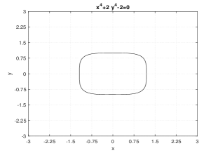
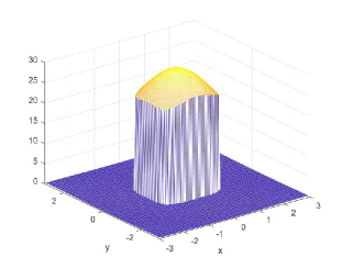
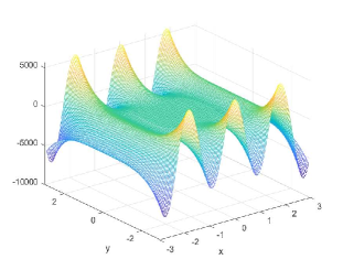
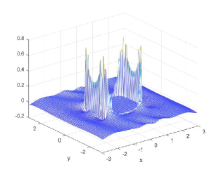
Figure 5. Top row for Example 1: the interface curve $\Gamma$ (left), the coefficient $a(x,y)$ (middle) and the numerical solution $u_{h}$ (right) with $h=2^{-7}\times 6$. Bottom row for Example 1: the error $u_{h}-u$ (left), the numerical $(u_{h})_{x}$ (middle) and the error $(u_{h})_{x}-u_{x}$ (right) with $h=2^{-7}\times 6$.

Example 2.

Let $\Omega=(-\pi,\pi)^{2}$ and the interface curve be given by $\Gamma:=\{(x,y)\in\Omega\;:\;\psi(x,y)=0\}$ with $\psi(x,y)=x^{2}+y^{2}-2$. Note that $\Gamma\cap\partial\Omega=\emptyset$, the coefficient $a$ and the exact solution $u$ of (1.1) are given by

$$a_{+}=a\chi_{\Omega^{+}}=\frac{2+\sin(x)\sin(y)}{100},\qquad a_{-}=a\chi_{\Omega^{-}}=10(2+\sin(x)\sin(y)),$$

$$u_{+}=u\chi_{\Omega^{+}}=100\sin(-2x)(x^{2}+y^{2}-2),\qquad u_{-}=u\chi_{\Omega^{-}}=\frac{\sin(-2x)(x^{2}+y^{2}-2)}{10}-100.$$

All the functions $f,g_{1},g_{2},g$ in (1.1) can be obtained by plugging the above coefficient and exact solution into (1.1). In particular, $g_{1}=100$ and $g_{2}=0$. The numerical results are presented in Table 2 and Fig. 6.

Table 2. Performance in Example 2 of the proposed high order compact finite difference scheme in Theorems 3.1, 4.1, 3.3 and 4.2 on uniform Cartesian meshes with $h=2^{-J}\times 2\pi$. $\kappa$ is the condition number of the coefficient matrix.

$J$	$\frac{\|u_{h}-u\|_{2,\Lambda_{\Omega}}}{\|u\|_{2,\Lambda_{\Omega},h}}$	order	$\frac{|u_{h}-u|_{H^{1},\Lambda_{\Omega}}}{|u|_{H^{1},\Lambda_{\Omega},h}}$	order	$\frac{|u_{h}-u|_{V,\Lambda_{\Omega}}}{|u|_{V,\Lambda_{\Omega},h}}$	order	$\kappa$
3	1.3309E+01	0	5.9842E+00	0	9.9219E+01	0	9.2851E+06
4	3.5796E-02	8.538	4.5479E-02	7.040	1.6452E-01	9.236	2.7593E+06
6	1.1989E-04	4.111	3.7322E-04	3.465	2.3716E-03	3.058	5.6730E+06
7	5.6264E-06	4.413	2.9690E-05	3.652	1.6035E-04	3.887	2.9228E+07
8	3.7420E-07	3.910	2.4650E-06	3.590	1.6760E-05	3.258	6.5794E+07

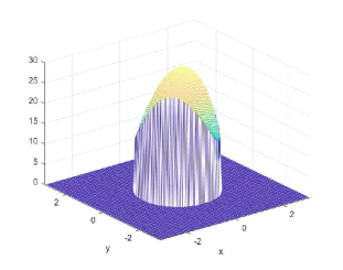
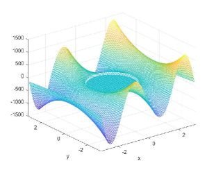
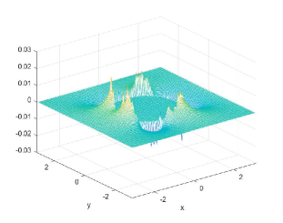
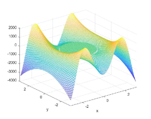
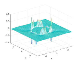
Figure 6. Top row for Example 2: the interface curve $\Gamma$ (left), the coefficient $a(x,y)$ (middle) and the numerical solution $u_{h}$ (right) with $h=2^{-7}\times 2\pi$. Bottom row for Example 2: the error $u_{h}-u$ (left), the numerical $(u_{h})_{x}$ (middle) and the error $(u_{h})_{x}-u_{x}$ (right) with $h=2^{-7}\times 2\pi$.

Example 3.

Let $\Omega=(-\pi,\pi)^{2}$ and the interface curve be given by $\Gamma:=\{(x,y)\in\Omega\;:\;\psi(x,y)=0\}$ with $\psi(x,y)=y^{2}-2x^{2}+x^{4}-1$. Note that $\Gamma\cap\partial\Omega=\emptyset$, the coefficient $a$ and the exact solution $u$ of (1.1) are given by

$$a_{+}=a\chi_{\Omega^{+}}=10(10+\sin(x+y)),\qquad a_{-}=a\chi_{\Omega^{-}}=\frac{10+\sin(x+y)}{1000},$$

$$u_{+}=u\chi_{\Omega^{+}}=\frac{\sin(2y)(y^{2}-2x^{2}+x^{4}-1)}{10},\qquad u_{-}=u\chi_{\Omega^{-}}=1000\sin(2y)(y^{2}-2x^{2}+x^{4}-1)+100.$$

All the functions $f,g_{1},g_{2},g$ in (1.1) can be obtained by plugging the above coefficient and exact solution into (1.1). In particular, $g_{1}=-100$ and $g_{2}=0$. The numerical results are presented in Table 3 and Fig. 7.

Table 3. Performance in Example 3 of the proposed high order compact finite difference scheme in Theorems 3.1, 4.1, 3.3 and 4.2 on uniform Cartesian meshes with $h=2^{-J}\times 2\pi$. $\kappa$ is the condition number of the coefficient matrix.

$J$	$\frac{\|u_{h}-u\|_{2,\Lambda_{\Omega}}}{\|u\|_{2,\Lambda_{\Omega},h}}$	order	$\frac{|u_{h}-u|_{H^{1},\Lambda_{\Omega}}}{|u|_{H^{1},\Lambda_{\Omega},h}}$	order	$\frac{|u_{h}-u|_{V,\Lambda_{\Omega}}}{|u|_{V,\Lambda_{\Omega},h}}$	order	$\kappa$
3	6.1884E+01	0	3.9779E+01	0	6.7918E+00	0	9.9817E+05
4	4.9790E-01	6.958	1.0408E+00	5.256	2.7858E-01	4.608	2.6762E+05
5	3.3387E-02	3.899	2.0705E-01	2.330	3.9791E-02	2.808	3.8920E+04
6	1.5988E-03	4.384	7.9473E-03	4.703	3.6630E-03	3.441	8.2465E+04
7	1.0671E-04	3.905	5.1411E-04	3.950	2.9131E-04	3.652	1.7768E+05
8	7.5627E-06	3.819	4.1588E-04	0.306	3.2258E-05	3.175	4.1282E+05

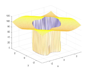
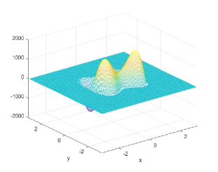
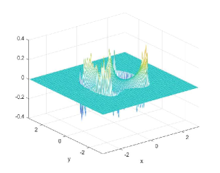
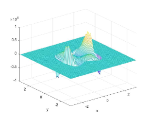
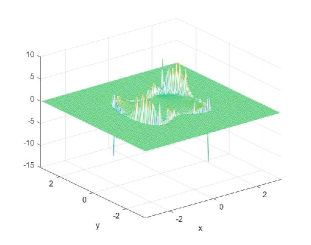
Figure 7. Top row for Example 3: the interface curve $\Gamma$ (left), the coefficient $a(x,y)$ (middle) and the numerical solution $u_{h}$ (right) with $h=2^{-7}\times 2\pi$. Bottom row for Example 3: the error $u_{h}-u$ (left), the numerical $(u_{h})_{x}$ (middle) and the error $(u_{h})_{x}-u_{x}$ (right) with $h=2^{-7}\times 2\pi$.

Example 4.

Let $\Omega=(-2.5,2.5)^{2}$ and the interface curve be given by $\Gamma:=\{(x,y)\in\Omega\;:\;\psi(x,y)=0\}$ with $\psi(x,y)=2x^{4}+y^{2}-1/2$. Note that $\Gamma\cap\partial\Omega=\emptyset$, the coefficient $a$ and the exact solution $u$ of (1.1) are given by

$$a_{+}=a\chi_{\Omega^{+}}=10(\exp(x-y)),\qquad a_{-}=a\chi_{\Omega^{-}}=\frac{\exp(x-y)}{1000},$$

$$u_{+}=u\chi_{\Omega^{+}}=\frac{\cos(4x)(2x^{4}+y^{2}-1/2)}{10},\qquad u_{-}=u\chi_{\Omega^{-}}=1000\cos(4x)(2x^{4}+y^{2}-1/2)+100.$$

All the functions $f,g_{1},g_{2},g$ in (1.1) can be obtained by plugging the above coefficient and exact solution into (1.1). In particular, $g_{1}=-100$ and $g_{2}=0$. The numerical results are presented in Table 4 and Fig. 8.

Table 4. Performance in Example 4 of the proposed high order compact finite difference scheme in Theorems 3.1, 4.1, 3.3 and 4.2 on uniform Cartesian meshes with $h=2^{-J}\times 5$. $\kappa$ is the condition number of the coefficient matrix.

$J$	$\frac{\|u_{h}-u\|_{2,\Lambda_{\Omega}}}{\|u\|_{2,\Lambda_{\Omega},h}}$	order	$\frac{|u_{h}-u|_{H^{1},\Lambda_{\Omega}}}{|u|_{H^{1},\Lambda_{\Omega},h}}$	order	$\frac{|u_{h}-u|_{V,\Lambda_{\Omega}}}{|u|_{V,\Lambda_{\Omega},h}}$	order	$\kappa$
3	2.1935E+02	0	4.7152E+04	0	2.7271E+01	0	1.1680E+08
4	2.5293E+00	6.438	1.7464E+00	14.721	7.9277E-02	8.426	1.6969E+04
5	4.0984E-01	2.626	1.0324E+00	0.758	5.1915E-03	3.933	6.9287E+04
6	3.6886E-02	3.474	4.9797E-02	4.374	3.0372E-04	4.095	5.8211E+04
7	2.2165E-03	4.057	4.3521E-03	3.516	1.7765E-05	4.096	4.8458E+04
8	1.3130E-04	4.077	3.8261E-04	3.508	1.7755E-06	3.323	1.4692E+05

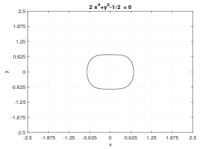
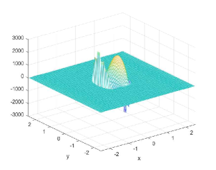
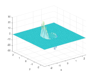
Figure 8. Top row for Example 4: the interface curve $\Gamma$ (left), the coefficient $a(x,y)$ (middle) and the numerical solution $u_{h}$ (right) with $h=2^{-7}\times 5$. Bottom row for Example 4: the error $u_{h}-u$ (left), the numerical $(u_{h})_{x}$ (middle) and the error $(u_{h})_{x}-u_{x}$ (right) with $h=2^{-7}\times 5$.

Example 5.

Let $\Omega=(-\frac{2\pi}{3},\frac{2\pi}{3})^{2}$ and the interface curve be given by $\Gamma:=\{(x,y)\in\Omega\;:\;\psi(x,y)=0\}$ with $\psi(x,y)=y^{2}+\frac{2x^{2}}{x^{2}+1}-1$. Note that $\Gamma\cap\partial\Omega=\emptyset$, the coefficient $a$ and the exact solution $u$ of (1.1) are given by

$$a_{+}=a\chi_{\Omega^{+}}=100(2+\cos(x)\sin(y)),\qquad a_{-}=a\chi_{\Omega^{-}}=\frac{2+\cos(x)\sin(y)}{10},$$

$$u_{+}=u\chi_{\Omega^{+}}=\frac{\cos(4x)(y^{2}(x^{2}+1)+x^{2}-1)}{100},\qquad u_{-}=u\chi_{\Omega^{-}}=10\cos(4x)(y^{2}(x^{2}+1)+x^{2}-1)+100.$$

All the functions $f,g_{1},g_{2},g$ in (1.1) can be obtained by plugging the above coefficient and exact solution into (1.1). In particular, $g_{1}=-100$ and $g_{2}=0$. The numerical results are presented in Table 5 and Fig. 9.

Table 5. Performance in Example 5 of the proposed high order compact finite difference scheme in Theorems 3.1, 4.1, 3.3 and 4.2 on uniform Cartesian meshes with $h=2^{-J}\times\frac{4\pi}{3}$. $\kappa$ is the condition number of the coefficient matrix.

$J$	$\frac{\|u_{h}-u\|_{2,\Lambda_{\Omega}}}{\|u\|_{2,\Lambda_{\Omega},h}}$	order	$\frac{|u_{h}-u|_{H^{1},\Lambda_{\Omega}}}{|u|_{H^{1},\Lambda_{\Omega},h}}$	order	$\frac{|u_{h}-u|_{V,\Lambda_{\Omega}}}{|u|_{V,\Lambda_{\Omega},h}}$	order	$\kappa$
3	1.5378E-01	0	3.8692E+00	0	2.0796E+00	0	2.2711E+04
4	9.3482E-02	0.718	1.3359E+00	1.534	1.9525E-01	3.413	1.7331E+04
5	6.1310E-03	3.930	1.3409E-01	3.317	2.1612E-02	3.175	1.6113E+04
6	2.9209E-04	4.392	1.0776E-02	3.637	3.5076E-03	2.623	3.8570E+04
7	1.4985E-05	4.285	8.2753E-04	3.703	3.0513E-04	3.523	2.9413E+04
8	1.3087E-06	3.517	9.3813E-05	3.141	3.4585E-05	3.141	6.0381E+04

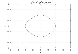
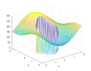
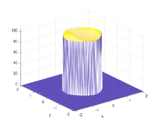
Figure 9. Top row for Example 5: the interface curve $\Gamma$ (left), the coefficient $a(x,y)$ (middle) and the numerical solution $u_{h}$ (right) with $h=2^{-7}\times\frac{4\pi}{3}$. Bottom row for Example 5: the error $u_{h}-u$ (left), the numerical $(u_{h})_{x}$ (middle) and the error $(u_{h})_{x}-u_{x}$ (right) with $h=2^{-7}\times\frac{4\pi}{3}$.

5.2. Numerical examples with $u$ unknown and $\Gamma\cap\partial\Omega=\emptyset$

In this subsection, we provide 5 numerical experiments such that the exact solution $u$ of (1.1) is unknown.

Example 6.

Let $\Omega=(-\pi,\pi)^{2}$ and the interface curve be given by $\Gamma:=\{(x,y)\in\Omega\;:\;\psi(x,y)=0\}$ with $\psi(x,y)=x^{4}+2y^{4}-2$. Note that $\Gamma\cap\partial\Omega=\emptyset$ and (1.1) is given by

$$a_{+}=a\chi_{\Omega^{+}}=100(2+\sin(x)\cos(y)),\qquad a_{-}=a\chi_{\Omega^{-}}=\frac{2+\sin(x)\cos(y)}{10},$$

$$f_{+}=f\chi_{\Omega^{+}}=\sin(2x)\sin(2y),\qquad f_{-}=f\chi_{\Omega^{-}}=\cos(2x)\cos(2y),$$

$$g_{1}=\exp(x-y)-10,\qquad g_{2}=\cos(x+y),\qquad g=0.$$

The numerical results are provided in Table 6 and Fig. 10.

Table 6. Performance in Example 6 of the proposed high order compact finite difference scheme in Theorems 3.1, 4.1, 3.3 and 4.2 on uniform Cartesian meshes with $h=2^{-J}\times 2\pi$. $\kappa$ is the condition number of the coefficient matrix.

$J$	$\|u_{h}-u_{h/2}\|_{2,\Lambda_{\Omega}}$	order	$|u_{h}-u_{h/2}|_{H^{1},\Lambda_{\Omega}}$	order	$|u_{h}-u_{h/2}|_{V,\Lambda_{\Omega}}$	order	$\kappa$
3	2.8284E-01	0	1.4650E+01	0	1.2366E+01	0	7.8789E+02
4	5.3709E-02	2.397	3.6196E-01	5.339	2.6415E+00	2.227	2.7310E+03
5	6.6858E-03	3.006	7.6924E-02	2.234	8.3040E-01	1.669	8.7219E+03
6	3.9281E-04	4.089	5.4377E-03	3.822	6.2964E-02	3.721	4.5222E+04
7	2.0733E-05	4.244	3.2159E-04	4.080	5.2101E-03	3.595	2.2395E+04

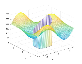
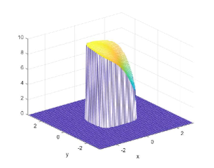
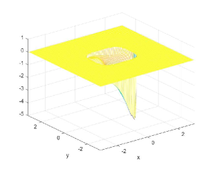
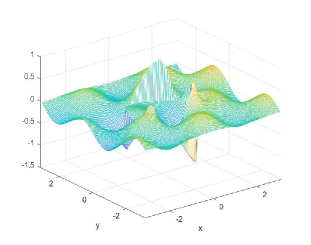
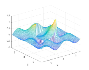
Figure 10. Top row for Example 6: the interface curve $\Gamma$ (left), the coefficient $a(x,y)$ (middle) and the numerical solution $u_{h}$ (right) with $h=2^{-7}\times 2\pi$. Bottom row for Example 6: the numerical $(u_{h})_{x}$ (left), the numerical $a(x,y)\times(u_{h})_{x}$ (middle) and the numerical $a(x,y)\times(u_{h})_{y}$ (right) with $h=2^{-7}\times 2\pi$.

Example 7.

Let $\Omega=(-\pi,\pi)^{2}$ and the interface curve be given by $\Gamma:=\{(x,y)\in\Omega\;:\;\psi(x,y)=0\}$ with $\psi(x,y)=y^{2}-2x^{2}+x^{4}-1$. Note that $\Gamma\cap\partial\Omega=\emptyset$ and (1.1) is given by

$$a_{+}=a\chi_{\Omega^{+}}=\frac{10}{2+\cos(x+y)},\qquad a_{-}=a\chi_{\Omega^{-}}=\frac{2+\sin(x+y)}{100},$$

$$f_{+}=f\chi_{\Omega^{+}}=\sin(2x)\sin(y),\qquad f_{-}=f\chi_{\Omega^{-}}=\exp(x+y)\sin(x),$$

$$g_{1}=\cos(x-y)-1,\qquad g_{2}=\sin(x-y),\qquad g=0.$$

The numerical results are provided in Table 7 and Fig. 11.

Table 7. Performance in Example 7 of the proposed high order compact finite difference scheme in Theorems 3.1, 4.1, 3.3 and 4.2 on uniform Cartesian meshes with $h=2^{-J}\times 2\pi$. $\kappa$ is the condition number of the coefficient matrix.

$J$	$\|u_{h}-u_{h/2}\|_{2,\Lambda_{\Omega}}$	order	$|u_{h}-u_{h/2}|_{H^{1},\Lambda_{\Omega}}$	order	$|u_{h}-u_{h/2}|_{V,\Lambda_{\Omega}}$	order	$\kappa$
3	2.4355E+03	0	5.4333E+03	0	1.9856E+03	0	8.2409E+05
4	1.0396E+01	7.872	3.3857E+02	4.004	9.7875E+00	7.664	4.3788E+03
5	5.4539E-01	4.253	1.1565E+01	4.872	6.0239E-01	4.022	6.5855E+03
6	3.3619E-02	4.020	2.7956E-01	5.370	7.6827E-02	2.971	4.3061E+03
7	2.1505E-03	3.967	2.1704E-02	3.687	5.4389E-03	3.820	1.3806E+04

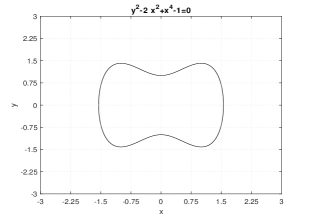
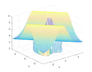
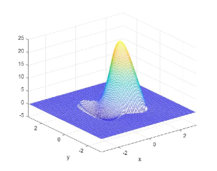
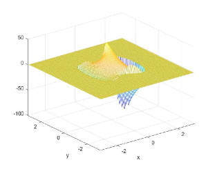
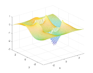
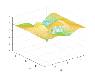
Figure 11. Top row for Example 7: the interface curve $\Gamma$ (left), the coefficient $a(x,y)$ (middle) and the numerical solution $u_{h}$ (right) with $h=2^{-7}\times 2\pi$. Bottom row for Example 7: the numerical $(u_{h})_{x}$ (left), the numerical $a(x,y)\times(u_{h})_{x}$ (middle) and the numerical $a(x,y)\times(u_{h})_{y}$ (right) with $h=2^{-7}\times 2\pi$.

Example 8.

Let $\Omega=(-2,2)^{2}$ and the interface curve be given by $\Gamma:=\{(x,y)\in\Omega\;:\;\psi(x,y)=0\}$ with $\psi(x,y)=2x^{4}+y^{2}-1/2$. Note that $\Gamma\cap\partial\Omega=\emptyset$ and (1.1) is given by

$$a_{+}=a\chi_{\Omega^{+}}=100(2+\sin(x)\cos(y)),\qquad a_{-}=a\chi_{\Omega^{-}}=\frac{2+\cos(x-y)}{10},$$

$$f_{+}=f\chi_{\Omega^{+}}=\sin(\pi x)\sin(\pi y),\qquad f_{-}=f\chi_{\Omega^{-}}=\cos(\pi x)\cos(\pi y),$$

$$g_{1}=\sin(x)\cos(y)-2,\qquad g_{2}=\cos(x)\sin(y),\qquad g=0.$$

The numerical results are provided in Table 8 and Fig. 12.

Table 8. Performance in Example 8 of the proposed high order compact finite difference scheme in Theorems 3.1, 4.1, 3.3 and 4.2 on uniform Cartesian meshes with $h=2^{-J}\times 4$. $\kappa$ is the condition number of the coefficient matrix.

$J$	$\|u_{h}-u_{h/2}\|_{2,\Lambda_{\Omega}}$	order	$|u_{h}-u_{h/2}|_{H^{1},\Lambda_{\Omega}}$	order	$|u_{h}-u_{h/2}|_{V,\Lambda_{\Omega}}$	order	$\kappa$
3	1.9911E-01	0	5.6734E+00	0	4.7783E+00	0	6.3170E+02
4	1.7085E-02	3.543	1.9762E-01	4.843	2.3331E+00	1.034	1.0358E+04
5	1.7892E-03	3.255	9.9839E-03	4.307	9.2170E-02	4.662	2.6379E+03
6	1.0570E-04	4.081	9.6792E-04	3.367	8.5957E-03	3.423	4.3995E+03
7	6.3279E-06	4.062	8.2529E-05	3.552	6.2430E-04	3.783	1.4608E+04

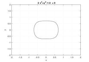
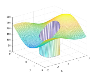
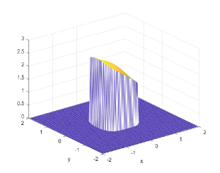
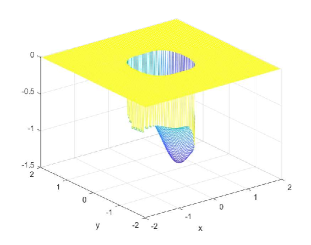
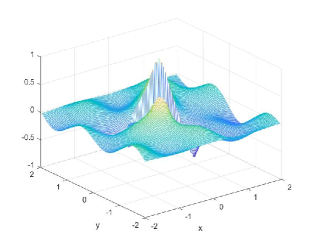
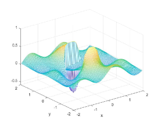
Figure 12. Top row for Example 8: the interface curve $\Gamma$ (left), the coefficient $a(x,y)$ (middle) and the numerical solution $u_{h}$ (right) with $h=2^{-7}\times 4$. Bottom row for Example 8: the numerical $(u_{h})_{x}$ (left), the numerical $a(x,y)\times(u_{h})_{x}$ (middle) and the numerical $a(x,y)\times(u_{h})_{y}$ (right) with $h=2^{-7}\times 4$.

Example 9.

Let $\Omega=(-\pi,\pi)^{2}$ and the interface curve be given by $\Gamma:=\{(x,y)\in\Omega\;:\;\psi(x,y)=0\}$ with $\psi(x,y)=x^{2}+y^{2}-2$. Note that $\Gamma\cap\partial\Omega=\emptyset$ and (1.1) is given by

$$a_{+}=a\chi_{\Omega^{+}}=\frac{10+\sin(x)\cos(y)}{100},\qquad a_{-}=a\chi_{\Omega^{-}}=10(10+\sin(x-y)),$$

$$f_{+}=f\chi_{\Omega^{+}}=\sin(2x)\sin(2y),\qquad f_{-}=f\chi_{\Omega^{-}}=\sin(2x)\sin(2y),$$

$$g_{1}=\sin(x)\sin(y)+2,\qquad g_{2}=\cos(y),\qquad g=0.$$

The numerical results are provided in Table 9 and Fig. 13.

Table 9. Performance in Example 9 of the proposed high order compact finite difference scheme in Theorems 3.1, 4.1, 3.3 and 4.2 on uniform Cartesian meshes with $h=2^{-J}\times 2\pi$. $\kappa$ is the condition number of the coefficient matrix.

$J$	$\|u_{h}-u_{h/2}\|_{2,\Lambda_{\Omega}}$	order	$|u_{h}-u_{h/2}|_{H^{1},\Lambda_{\Omega}}$	order	$|u_{h}-u_{h/2}|_{V,\Lambda_{\Omega}}$	order	$\kappa$
3	3.6443E+01	0	2.6368E+01	0	5.5413E+01	0	3.5485E+06
4	3.3319E+00	3.451	2.5138E+00	3.391	9.4984E-01	5.866	4.2304E+06
5	5.1908E-01	2.682	3.9809E-01	2.659	9.3815E-01	0.018	2.0691E+09
6	4.4040E-02	3.559	3.4551E-02	3.526	1.0907E-02	6.426	4.4599E+06
7	1.5339E-03	4.844	1.4934E-03	4.532	7.1251E-04	3.936	1.5863E+07

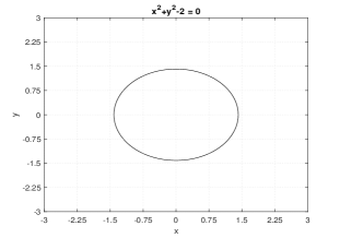
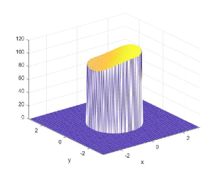
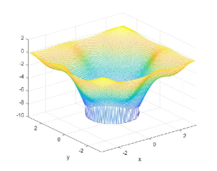
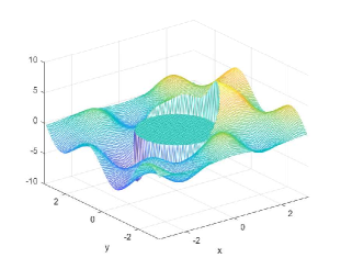
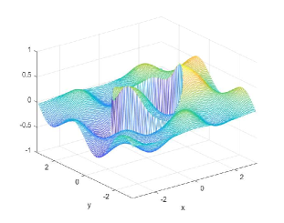
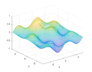
Figure 13. Top row for Example 9: the interface curve $\Gamma$ (left), the coefficient $a(x,y)$ (middle) and the numerical solution $u_{h}$ (right) with $h=2^{-7}\times 2\pi$. Bottom row for Example 9: the numerical $(u_{h})_{x}$ (left), the numerical $a(x,y)\times(u_{h})_{x}$ (middle) and the numerical $a(x,y)\times(u_{h})_{y}$ (right) with $h=2^{-7}\times 2\pi$.

Example 10.

Let $\Omega=(-2,2)^{2}$ and the interface curve be given by $\Gamma:=\{(x,y)\in\Omega\;:\;\psi(x,y)=0\}$ with $\psi(x,y)=2x^{4}+y^{2}-1/2$. Note that $\Gamma\cap\partial\Omega=\emptyset$ and (1.1) is given by

$$a_{+}=a\chi_{\Omega^{+}}=\frac{10+\sin(x)\cos(y)}{100},\qquad a_{-}=a\chi_{\Omega^{-}}=10(10+\cos(x-y)),$$

$$f_{+}=f\chi_{\Omega^{+}}=\sin(\pi x)\sin(\pi y),\qquad f_{-}=f\chi_{\Omega^{-}}=\sin(\pi x)\sin(\pi y),$$

$$g_{1}=-\sin(x)\sin(y)-2,\qquad g_{2}=-\cos(y),\qquad g=0.$$

The numerical results are provided in Table 10 and Fig. 14.

Table 10. Performance in Example 10 of the proposed high order compact finite difference scheme in Theorems 3.1, 4.1, 3.3 and 4.2 on uniform Cartesian meshes with $h=2^{-J}\times 4$. $\kappa$ is the condition number of the coefficient matrix.

$J$	$\|u_{h}-u_{h/2}\|_{2,\Lambda_{\Omega}}$	order	$|u_{h}-u_{h/2}|_{H^{1},\Lambda_{\Omega}}$	order	$|u_{h}-u_{h/2}|_{V,\Lambda_{\Omega}}$	order	$\kappa$
3	1.0502E+02	0	1.0875E+02	0	1.4944E+03	0	1.3769E+05
4	4.1249E+00	4.670	4.9993E+00	4.443	1.9580E+01	6.254	5.5506E+04
5	1.1253E+00	1.874	1.3475E+00	1.891	2.0402E-01	6.585	3.6392E+06
6	8.9752E-02	3.648	1.0730E-01	3.651	3.3886E-02	2.590	1.7678E+08
7	6.5737E-03	3.771	7.9995E-03	3.746	2.4428E-03	3.794	1.9945E+07

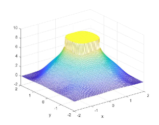
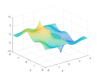
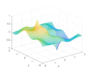
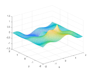
Figure 14. Top row for Example 10: the interface curve $\Gamma$ (left), the coefficient $a(x,y)$ (middle) and the numerical solution $u_{h}$ (right) with $h=2^{-7}\times 4$. Bottom row for Example 10: the numerical $(u_{h})_{x}$ (left), the numerical $a(x,y)\times(u_{h})_{x}$ (middle) and the numerical $a(x,y)\times(u_{h})_{y}$ (right) with $h=2^{-7}\times 4$.

6. Conclusion

To our best knowledge, so far there is only one fourth order compact finite difference scheme for the numerical approximated solution for the interface elliptic problems with piecewise constant coefficients, continuous source terms and two homogeneous jump conditions in [17, Section 7.2.7] and [17, Section 7.5.4] provides the numerical results with $|a_{+}-a_{-}|=99$ or 9 for the proposed fourth order compact scheme in uniform and no-nested mesh grids. The compact schemes in [17, Section 7.2.7] are based on coordinate transformations and optimization problems.

Our contributions of this paper are as follows:

1. We construct a high order compact finite difference scheme for the numerical solution on uniform meshes for (1.1) with a discontinuous, piecewise smooth and high-contrast coefficient (the ratio $\sup(a_{+})/\inf(a_{-})=10^{-3},10^{-2},10^{3},10^{4}$), discontinuous source terms and two non-homogeneous jump conditions. $a_{+}$ and $a_{-}$ can be linearly independent or dependent.

2. Since we do not need to change coordinates into the local coordinates and solve an optimization problem to derive the scheme, it is simple for readers to understand the procedure, derive the schemes, and perform the implementations.

3. For the irregular points case, Eq.(7.73) in [17, Section 7.2.7] expands the Taylor series of $u(x,y)$ to $\mathcal{O}(h^{5})$, while we only need to expand the Taylor series of $u(x,y)$ to $\mathcal{O}(h^{4})$, which significantly reduces the computational costs to calculate the coefficients of the proposed schemes. Moreover, we also prove that the maximum order of the compact finite difference schemes for the numerical approximated solutions at irregular points on uniform meshes is three.

4. Since the gradients are crucial in the real world problems to analyze the speeds of fluids, we also derive a high order compact finite difference scheme for the numerical approximated gradients. Our numerical experiments confirm the flexibility and the fourth order accuracy in numerical approximated $L^{2}$ norms for the numerical approximated solutions $u_{h}$, the numerical approximated gradients $\big{(}(u_{h})_{x},(u_{h})_{y}\big{)}$ and the numerical approximated velocities $\big{(}a(u_{h})_{x},a(u_{h})_{y}\big{)}$ of the proposed schemes.

7. Proof of Theorem 3.2

Proof of Theorem 3.2.

Similar as the proof of Theorem 2.3 in [9], by (3.23), two jump conditions in (1.1) can be written as

$$u_{+}(r(t)+x_{i}^{*},s(t)+y_{j}^{*})-u_{-}(r(t)+x_{i}^{*},s(t)+y_{j}^{*})=g_{1}(r(t)+x_{i}^{*},s(t)+y_{j}^{*}),$$ (7.1)

$$\begin{split}\big{(}(a_{+}\nabla u_{+})(r(t)+x_{i}^{*},s(t)+y_{j}^{*})-&(a_{-}\nabla u_{-})(r(t)+x_{i}^{*},s(t)+y_{j}^{*})\big{)}\cdot(s^{\prime}(t),-r^{\prime}(t))\\ &=g_{2}(r(t)+x_{i}^{*},s(t)+y_{j}^{*})\sqrt{(r^{\prime}(t))^{2}+(s^{\prime}(t))^{2}},\end{split}$$ (7.2)

for $t\in(-\epsilon,\epsilon)$. Because all involved functions in (7.1) and (7.2) are assumed to be smooth, to link the two sets $\{u_{+}^{(m,n)}:(m,n)\in\Lambda_{M+1}^{1}\}$ and $\{u_{-}^{(m,n)}:(m,n)\in\Lambda_{M+1}^{1}\}$, we now take the Taylor approximation of the above functions near the base parameter $t=0$. (3.19) implies

$$u_{\pm}(r(t)+x_{i}^{*},s(t)+y_{j}^{*}) =\sum_{(m,n)\in\Lambda_{M+1}^{1}}u_{\pm}^{(m,n)}G^{\pm}_{m,n}(r(t),s(t))+\sum_{(m,n)\in\Lambda_{M-1}}f_{\pm}^{(m,n)}H^{\pm}_{m,n}(r(t),s(t))+\mathcal{O}(t^{M+2})$$

$$=\sum_{p=0}^{M+1}\left(\sum_{(m,n)\in\Lambda_{M+1}^{1}}u_{\pm}^{(m,n)}g^{\pm}_{m,n,p}+\sum_{(m,n)\in\Lambda_{M-1}}f_{\pm}^{(m,n)}h^{\pm}_{m,n,p}\right)t^{p}+\mathcal{O}(t^{M+2}),$$

where

$$g^{\pm}_{m,n,p}:=\frac{1}{p!}\frac{d^{p}(G^{\pm}_{m,n}(r(t),s(t)))}{dt^{p}}\Big{|}_{t=0},\ \ h^{\pm}_{m,n,p}:=\frac{1}{p!}\frac{d^{p}(H^{\pm}_{m,n}(r(t),s(t)))}{dt^{p}}\Big{|}_{t=0},\quad p=0,\ldots,M+1.$$ (7.3)

Similarly,

$$g_{1}(r(t)+x_{i}^{*},s(t)+y_{j}^{*}) =\sum_{(m,n)\in\Lambda_{M+1}}\frac{g_{1}^{(m,n)}}{m!n!}(r(t))^{m}(s(t))^{n}+\mathcal{O}(t^{M+2})$$

$$=\sum_{p=0}^{M+1}\left(\sum_{(m,n)\in\Lambda_{M+1}}\frac{g_{1}^{(m,n)}}{m!n!}r_{m,n,p}\right)t^{p}+\mathcal{O}(t^{M+2}),$$

where the constants $r_{m,n,p}:=\frac{1}{p!}\frac{d^{p}((r(t))^{m}(s(t))^{n})}{dt^{p}}\Big{|}_{t=0}$ for $p=0,\ldots,M+1$. Since each entry of ${G}^{\pm}_{m,n}(x,y)$ is a homogeneous polynomial of degree $\geq m+n$ and $r(0)=s(0)=0$, we have $g^{\pm}_{m,n,p}=0$ for all $0\leq p<m+n$ by (7.3). Thus, (7.1) leads to

$$\sum_{(m,n)\in\Lambda_{M+1}^{1}}u_{+}^{(m,n)}g^{+}_{m,n,p}-u_{-}^{(m,n)}g^{-}_{m,n,p}=F_{p},\qquad p=0,\ldots,M+1,$$ (7.4)

where $F_{0}:=g_{1}^{(0,0)}$ and

$$F_{p}:=\sum_{(m,n)\in\Lambda_{M-1}}f_{-}^{(m,n)}h^{-}_{m,n,p}-f_{+}^{(m,n)}h^{+}_{m,n,p}+\sum_{(m,n)\in\Lambda_{M+1}}\frac{g_{1}^{(m,n)}}{m!n!}r_{m,n,p},\qquad p=1,\ldots,M+1.$$

Clearly, $g^{\pm}_{0,0,0}=1$ and $g^{\pm}_{m,n,p}=0$ for all $0\leq p<m+n$. We observe that the identities in (7.4) become

$$u_{-}^{(0,0)}=u_{+}^{(0,0)}-g_{1}^{(0,0)},$$ (7.5)

$$\begin{split}&u_{-}^{(0,p)}g^{-}_{0,p,p}+u_{-}^{(1,p-1)}g^{-}_{1,p-1,p}=u_{+}^{(0,p)}g^{+}_{0,p,p}+u_{+}^{(1,p-1)}g^{+}_{1,p-1,p}-F_{p}\\ &+\sum_{(m,n)\in\Lambda_{p-1}^{1}}u_{+}^{(m,n)}g^{+}_{m,n,p}-u_{-}^{(m,n)}g^{-}_{m,n,p},\qquad p=1,\ldots,M+1.\end{split}$$ (7.6)

By (2.11),

$$G^{\pm}_{m,n}(x,y):=G^{\pm,1}_{m,n}(x,y)+G^{\pm,2}_{m,n}(x,y),$$ (7.7)

where

$$G^{\pm,1}_{m,n}(x,y):=\sum_{\ell=0}^{\lfloor\frac{n}{2}\rfloor}\frac{(-1)^{\ell}x^{m+2\ell}y^{n-2\ell}}{(m+2\ell)!(n-2\ell)!},$$ (7.8)

$$G^{\pm,2}_{m,n}(x,y):=\sum_{(m^{\prime},n^{\prime})\in\Lambda_{M+1}^{2}\setminus\Lambda_{m+n}^{2}}A^{u}_{m^{\prime},n^{\prime},m,n}\frac{x^{m^{\prime}}y^{n^{\prime}}}{m^{\prime}!n^{\prime}!},\quad\forall(m,n)\in\Lambda_{M+1}^{1}.$$ (7.9)

Since each entry of $G^{\pm,2}_{m,n}(x,y)$ is a homogeneous polynomial of degree $\geq m+n+1$ and $s(0)=r(0)=0$, (7.3) leads to

$$g^{\pm}_{m,n,p}:=\frac{1}{p!}\frac{d^{p}(G^{\pm,1}_{m,n}(r(t),s(t)))}{dt^{p}}\Big{|}_{t=0},\quad(m,n)\in\{(0,p),(1,p-1)\}.$$ (7.10)

For the flux jump condition (7.2), (3.19) implies

$$\begin{split}\nabla\big{(}u_{\pm}(x+x_{i}^{*},y+y_{j}^{*}))\big{)}&=\sum_{(m,n)\in\Lambda_{M+1}^{1}}u_{\pm}^{(m,n)}\nabla\big{(}G^{\pm}_{m,n}(x,y)\big{)}+\sum_{(m,n)\in\Lambda_{M-1}}f_{\pm}^{(m,n)}\nabla\big{(}H^{\pm}_{m,n}(x,y)\big{)}+\mathcal{O}(h^{M+1}),\end{split}$$ (7.11)

for $x,y\in(-2h,2h)$ and clearly

$$a_{\pm}(x+x_{i}^{*},y+y_{j}^{*})=\sum_{(m,n)\in\Lambda_{M}}\frac{a_{\pm}^{(m,n)}}{m!n!}x^{m}y^{n}+\mathcal{O}(h^{M+1}),$$ (7.12)

for $x,y\in(-2h,2h)$. By (7.11) and (7.12),

$$a_{\pm}(x+x_{i}^{*},y+y_{j}^{*})\nabla u_{\pm}(r(t)+x_{i}^{*},s(t)+y_{j}^{*})\cdot(s^{\prime}(t),-r^{\prime}(t))$$

$$=\sum_{(m,n)\in\Lambda_{M+1}^{1}}u_{\pm}^{(m,n)}\widetilde{G}^{\pm}_{m,n}(r(t),s(t))\cdot(s^{\prime}(t),-r^{\prime}(t))+\sum_{(m,n)\in\Lambda_{M-1}}f_{\pm}^{(m,n)}\widetilde{H}^{\pm}_{m,n}(r(t),s(t))\cdot(s^{\prime}(t),-r^{\prime}(t))$$

$$=\sum_{p=0}^{M}\left(\sum_{(m,n)\in\Lambda_{M+1}^{1}}u_{\pm}^{(m,n)}\tilde{g}^{\pm}_{m,n,p}+\sum_{(m,n)\in\Lambda_{M-1}}f_{\pm}^{(m,n)}\tilde{h}^{\pm}_{m,n,p}\right)t^{p}+\mathcal{O}(t^{M+1}),$$

where

$$\widetilde{G}^{\pm}_{m,n}(x,y)=\nabla G^{\pm}_{m,n}(x,y)\Bigg{(}\sum_{(m,n)\in\Lambda_{M}}\frac{a_{\pm}^{(m,n)}}{m!n!}x^{m}y^{n}\Bigg{)},\ \ \widetilde{H}^{\pm}_{m,n}(x,y)=\nabla H^{\pm}_{m,n}(x,y)\Bigg{(}\sum_{(m,n)\in\Lambda_{M}}\frac{a_{\pm}^{(m,n)}}{m!n!}x^{m}y^{n}\Bigg{)},$$

$$\tilde{g}^{\pm}_{m,n,p}:=\frac{1}{p!}\frac{d^{p}(\widetilde{G}^{\pm}_{m,n}(r(t),s(t))\cdot(s^{\prime}(t),-r^{\prime}(t)))}{dt^{p}}\Big{|}_{t=0},\ \ \tilde{h}^{\pm}_{m,n,p}:=\frac{1}{p!}\frac{d^{p}(\widetilde{H}^{\pm}_{m,n}(r(t),s(t))\cdot(s^{\prime}(t),-r^{\prime}(t)))}{dt^{p}}\Big{|}_{t=0}.$$ (7.13)

Note that each entry of $\widetilde{G}^{\pm}_{m,n}$ is a homogeneous polynomial of degree $\geq m+n-1$. By $r(0)=s(0)=0$ and (7.13), we can say that $\tilde{g}^{\pm}_{m,n,p}=0$ for all $0\leq p<m+n-1$. Similarly, we have

$$g_{2}(r(t)+x_{i}^{*},s(t)+y_{j}^{*})\sqrt{(r^{\prime}(t))^{2}+(s^{\prime}(t))^{2}} =\sum_{(m,n)\in\Lambda_{M}}\frac{g_{2}^{(m,n)}}{m!n!}(r(t))^{m}(s(t))^{n}\sqrt{(r^{\prime}(t))^{2}+(s^{\prime}(t))^{2}}+\mathcal{O}(t^{M+1})$$

$$=\sum_{p=0}^{M}\left(\sum_{(m,n)\in\Lambda_{M}}\frac{g_{2}^{(m,n)}}{m!n!}\tilde{r}_{m,n,p}\right)t^{p}+\mathcal{O}(t^{M+1}),$$

as $t\to 0$, where

$$\tilde{r}_{m,n,p}:=\frac{1}{p!}\frac{d^{p}\Big{(}(r(t))^{m}(s(t))^{n}\sqrt{(r^{\prime}(t))^{2}+(s^{\prime}(t))^{2}}\Big{)}}{dt^{p}}\Bigg{|}_{t=0},\qquad p=0,\ldots,M.$$

Therefore, (7.2) implies

$$\sum_{(m,n)\in\Lambda_{M+1}^{1}}u_{+}^{(m,n)}\tilde{g}^{+}_{m,n,p}-u_{-}^{(m,n)}\tilde{g}^{-}_{m,n,p}=G_{p},\qquad p=0,\ldots,M,$$ (7.14)

where

$$G_{p}:=\sum_{(m,n)\in\Lambda_{M-1}}f_{-}^{(m,n)}\tilde{h}^{-}_{m,n,p}-f_{+}^{(m,n)}\tilde{h}^{+}_{m,n,p}+\sum_{(m,n)\in\Lambda_{M}}\frac{g_{2}^{(m,n)}}{m!n!}\tilde{r}_{m,n,p}.$$

Clearly, $\tilde{g}^{\pm}_{0,0,0}=0$ and $\tilde{g}^{\pm}_{m,n,p}=0$ for all $0\leq p<m+n-1$. We observe that (7.14) become

$$\begin{split}u_{-}^{(0,p)}\tilde{g}^{-}_{0,p,p-1}+u_{-}^{(1,p-1)}\tilde{g}^{-}_{1,p-1,p-1}&=u_{+}^{(0,p)}\tilde{g}^{+}_{0,p,p-1}+u_{+}^{(1,p-1)}\tilde{g}^{+}_{1,p-1,p-1}-G_{p-1}\\ &+\sum_{(m,n)\in\Lambda_{p-1}^{1}}u_{+}^{(m,n)}\tilde{g}^{+}_{m,n,p-1}-u_{-}^{(m,n)}\tilde{g}^{-}_{m,n,p-1},\quad p=1,\ldots,M+1.\end{split}$$ (7.15)

Since each entry of $G^{\pm,2}_{m,n}(x,y)$ is a homogeneous polynomial of degree $\geq m+n+1$ and $s(0)=r(0)=0$, (7.13) (7.7), (7.8) and (7.9) leads to

$$\tilde{g}^{\pm}_{m,n,p-1}:=\frac{a_{\pm}^{(0,0)}}{(p-1)!}\frac{d^{p-1}(\nabla G^{\pm,1}_{m,n}(x,y)\cdot(s^{\prime}(t),-r^{\prime}(t)))}{dt^{p-1}}\Big{|}_{t=0},\quad(m,n)\in\{(0,p),(1,p-1)\}.$$ (7.16)

According to the assumption $(r^{\prime}(0))^{2}+(s^{\prime}(0))^{2}>0$ in (3.23), $a_{\pm}^{(0,0)}\neq 0$ in (1.1) and the proof of Theorem 2.3 in [9], (7.8), (7.10) and (7.16) imply

$$g^{\pm}_{0,p,p}\tilde{g}^{\pm}_{1,p-1,p-1}-g^{\pm}_{1,p-1,p}\tilde{g}^{\pm}_{0,p,p-1}>0,\qquad\forall\;p=1,\ldots,M.$$ (7.17)

Let

$$W^{\pm}_{p}=\left[\begin{matrix}g^{\pm}_{0,p,p}&g^{\pm}_{1,p-1,p}\\ \tilde{g}^{\pm}_{0,p,p-1}&\tilde{g}^{\pm}_{1,p-1,p-1}\end{matrix}\right]\quad\mbox{and}\quad Q^{\pm}_{p}:=\frac{1}{g^{\pm}_{0,p,p}\tilde{g}^{\pm}_{1,p-1,p-1}-g^{\pm}_{1,p-1,p}\tilde{g}^{\pm}_{0,p,p-1}}\left[\begin{matrix}\tilde{g}^{\pm}_{1,p-1,p-1}&-g^{\pm}_{1,p-1,p}\\ -\tilde{g}^{\pm}_{0,p,p-1}&g^{\pm}_{0,p,p}\end{matrix}\right].$$

Then, by (7.17), we have $W^{\pm}_{p}Q^{\pm}_{p}=I_{2}$, where $I_{2}$ is a 2 by 2 identity matrix.

Therefore, the solution $\{u_{-}^{(0,p)},u_{-}^{(1,p-1)}\}_{p=1,\ldots M}$ of the linear equations in (7.6) and (7.15) can be recursively and uniquely calculated from $p=1$ to $p=M$ by $u_{-}^{(0,0)}=u_{+}^{(0,0)}-g_{1}^{(0,0)}$ due to (7.5) and

$$\begin{split}\left[\begin{matrix}u_{-}^{(0,p)}\\ u_{-}^{(1,p-1)}\end{matrix}\right]&=Q^{-}_{p}W^{+}_{p}\left[\begin{matrix}u_{+}^{(0,p)}\\ u_{+}^{(1,p-1)}\end{matrix}\right]-Q^{-}_{p}\left[\begin{matrix}F_{p}\\ G_{p-1}\end{matrix}\right]+\sum_{n=1}^{p-1}Q^{-}_{p}\left[\begin{matrix}u_{+}^{(0,n)}g^{+}_{0,n,p}+u_{+}^{(1,n-1)}g^{+}_{1,n-1,p}\\ u_{+}^{(0,n)}\tilde{g}^{+}_{0,n,p-1}+u_{+}^{(1,n-1)}\tilde{g}^{+}_{1,n-1,p-1}\end{matrix}\right]\\ &-\sum_{n=1}^{p-1}Q^{-}_{p}\left[\begin{matrix}u_{-}^{(0,n)}g^{-}_{0,n,p}+u_{-}^{(1,n-1)}g^{-}_{1,n-1,p}\\ u_{-}^{(0,n)}\tilde{g}^{-}_{0,n,p-1}+u_{-}^{(1,n-1)}\tilde{g}^{-}_{1,n-1,p-1}\end{matrix}\right],\end{split}$$ (7.18)

for $p=1,\ldots,M+1$. Note that for $p=1$, the above summation $\sum_{n=1}^{p-1}$ is empty. ∎

References

- [1] I. T. Angelova and L. G. Vulkov, High-order finite difference schemes for elliptic problems with intersecting interfaces. Appl. Math. Comput. 187 (2007), 824-843.
- [2] I. Babuška, The finite element method for elliptic equations with discontinuous coefficients. Computing. 5 (1970), 207-213.
- [3] J. H. Bramble and J. T. King, A finite element method for interface problems in domains with smooth boundaries and interfaces. Adv. Comput. Math. 6 (1996), 109-138.
- [4] G. Brandstetter and S. Govindjee, A high-order immersed boundary discontinuous-Galerkin method for Poisson’s equation with discontinuous coefficients and singular sources. Int. J. Numer. Methods. Eng. 101 (2015), no. 11, 847-869.
- [5] X. Chen, X. Feng and Z. Li, A direct method for accurate solution and gradient computations for elliptic interface problems. Numer. Algorithms. 80 (2019), 709-740.
- [6] B. Dong, X. Feng and Z. Li, An FE-FD method for anisotropic elliptic interface problems. SIAM J. Sci. Comput. 42 (2020), no. 4, B1041-B1066.
- [7] R. Ewing, Z. Li, T. Lin and Y. Lin, The immersed finite volume element methods for the elliptic interface problems. Math. Comput. Simul. 50 (1999), 63-76.
- [8] R. Ewing, O. Iliev and R. Lazarov, A modified finite volume approximation of second-order elliptic equations with discontinuous coefficients. SIAM J. Sci. Comput. 23 (2001), no. 4, 1335-1351.
- [9] Q. W. Feng, B. Han and P. Minev, Sixth order compact finite difference scheme for Poisson interface problem with singular sources. Preprint (2021).
- [10] Y. Gong, B. Li and Z. Li, Immersed-interface finite-element methods for elliptic interface problems with nonhomogeneous jump conditions. SIAM J. Numer. Anal. 46 (2008), no. 1, 472-495.
- [11] B. Guo and H. S. Oh, The h–p version of the finite element method for problems with interfaces. Int. J. Numer. Methods. Eng. 37 (1994), no. 10, 1741-1762.
- [12] B. Han, M. Michelle and Y. S. Wong, Dirac assisted tree method for 1D heterogeneous Helmholtz equations with arbitrary variable wave numbers. Preprint (2020).
- [13] A. Hansbo and P. Hansbo, An unfitted finite element method, based on Nitsche’s method, for elliptic interface problems. Comput. Methods Appl. Mech. Engrg. 191 (2002), no. 47-48, 5537-5552.
- [14] X. He, T. Lin and Y. Lin, Immersed finite element methods for elliptic interface problems with non-homogeneous jump conditions. Int. J. Numer. Anal. Model. 8 (2011), no. 2, 284-301.
- [15] K. Ito, Z. Li and Y. Kyei, Higher-Order, Cartesian Grid Based Finite Difference Schemes for Elliptic Equations on Irregular Domains. SIAM J. Sci. Comput. 27 (2005), no. 1, 346-367.
- [16] R. J. Leveque and Z. Li, The Immersed interface method for elliptic equations with discontinuous coefficients and singular sources. SIAM J. Numer. Anal. 31 (1994), no. 4, 1019-1044.
- [17] Z. Li and K. Ito, The immersed interface method: numerical solutions of PDEs involving interfaces and irregular domains. Society for Industrial and Applied Mathematics. 2006.
- [18] Z. Li, A fast iterative algorithm for elliptic interface problems. SIAM J. Numer. Anal. 35 (1998), no. 1, 230-254.
- [19] Z. Li, A note on immersed interface method for three-dimensional elliptic equations. Comput. Math. with Appl. 31 (1996), no. 3, 9-17.
- [20] T. Lin, Y. Lin and X. Zhang, Partially penalized immersed finite element methods for elliptic interface problems. SIAM J. Numer. Anal. 53 (2015), no. 2, 1121-1144.
- [21] T. Ma and Y. Ge, A higher-order blended compact difference (BCD) method for solving the general 2D linear second-order partial differential equation. Advances in Difference Equations. 98 (2019), 1-21.
- [22] T. Ma and Y. Ge, High-order blended compact difference schemes for the 3D elliptic partial differential equation with mixed derivatives and variable coefficients. Advances in Difference Equations. 525 (2020), 1-30.
- [23] A. C. Medina and R. Schmid, Solution of high order compact discretized 3D elliptic partial differential equations by an accelerated multigrid method. J. Comput. Appl. Math. 350 (2019), 343-352.
- [24] C. S. Peskin, The immersed boundary method. Acta Numerica (2002), 479-517.
- [25] S. O. Settle, C. C. Douglas, I. Kim, and D. Sheen, On the derivation of highest-order compact finite difference schemes for the one- and two-dimensional Poisson equation with Dirichlet boundary conditions. SIAM J. Numer. Anal. 51 (2013), no. 4, 2470-2490.
- [26] J. L. Vazquez, The Porous medium equation: mathematical theory. Clarendon Press. 2007. p15.
- [27] Y. Wang and J. Zhang, Sixth order compact scheme combined with multigrid method and extrapolation technique for 2D Poisson equation. J. Comput. Phys. 228 (2009), no. 1, 137-146.
- [28] Y. M. Wang, B. Y. Guo and W. J. Wu, Fourth-order compact finite difference methods and monotone iterative algorithms for semilinear elliptic boundary value problems. Comput. Math. with Appl. 68 (2014), 1671-1688.
- [29] A. Wiegmann and K. P. Bube, The explicit-jump immersed interface method: finite difference methods for PDEs with piecewise smooth solutions. SIAM J. Numer. Anal. 37 (2000), no. 3, 827-862.
- [30] S. Yu, Y. Zhou and G. W. Wei, Matched interface and boundary (MIB) method for elliptic problems with sharp-edged interfaces. J. Comput. Phys. 224 (2007), 729-756.
- [31] S. Yu and G. W. Wei, Three-dimensional matched interface and boundary (MIB) method for treating geometric singularities. J. Comput. Phys. 227 (2007), 602-632.
- [32] S. Zhai, X. Feng and Y. He, A family of fourth-order and sixth-order compact difference schemes for the three-dimensional Poisson equation. J. Sci. Comput. 54 (2013), 97-120.
- [33] J. Zhang, An explicit fourth-order compact finite difference scheme for three-dimensional convection-diffusion equation. Commun. Numer. Methods Eng. 14 (1998), 209-218.
- [34] Y. C. Zhou, S. Zhao, M. Feig and G. W. Wei, High order matched interface and boundary method for elliptic equations with discontinuous coefficients and singular sources. J. Comput. Phys. 213 (2006), no. 1, 1-30.