A Deep Dive into Conflict Generating Decisions

Abstract

Boolean Satisfiability (SAT) is a well-known NP-complete problem. Despite this theoretical hardness, SAT solvers based on Conflict Driven Clause Learning (CDCL) can solve large SAT instances from many important domains. CDCL learns clauses from conflicts, a technique that allows a solver to prune its search space. The selection heuristics in CDCL prioritize variables that are involved in recent conflicts. While only a fraction of decisions generate any conflicts, many generate multiple conflicts.

In this paper, we study conflict-generating decisions in CDCL in detail. We investigate the impact of single conflict (sc) decisions, which generate only one conflict, and multi-conflict (mc) decisions which generate two or more. We empirically characterize these two types of decisions based on the quality of the learned clauses produced by each type of decision. We also show an important connection between consecutive clauses learned within the same mc decision, where one learned clause triggers the learning of the next one forming a chain of clauses. This leads to the consideration of similarity between conflicts, for which we formulate the notion of conflictsproximity as a similarity measure. We show that conflicts in mc decisions are more closely related than consecutive conflicts generated from sc decisions. Finally, we develop Common Reason Variable Reduction (CRVR) as a new decision strategy that reduces the selection priority of some variables from the learned clauses of mc decisions. Our empirical evaluation of CRVR implemented in three leading solvers demonstrates performance gains in benchmarks from the main track of SAT Competition-2020.

1 Introduction

Boolean Satisfiability (SAT) is a fundamental problem in computer science, with strong relations to computational complexity, logic, and artificial intelligence. Given a formula $\mathcal{F}$ over boolean variables, a SAT solver either determines a variable assignment which satisfies $\mathcal{F}$, or reports unsatisfiability if no such assignment exists. In general, SAT solving is intractable [11]. Complete SAT solvers based on the framework of DPLL [12] employ heuristics-guided backtracking tree search. CDCL SAT solvers such as GRASP [27] and Chaff [22] substantially enhanced the DPLL framework by adding conflict analysis and clause learning.

Modern CDCL SAT solvers can solve very large real-world problem instances from important domains such as hardware design verification [14], software testing [8], automated planning [25], and encryption [21, 28]. The efficiency of modern solvers is the result of careful integration of their key components such as preprocessing [13, 15], inprocessing [16, 20], robust decision heuristics [17, 18, 22], efficient restart policies [7, 24], intelligent conflict analysis [27], and effective clause learning [22].

Clauses learned in CDCL can help prune the search space. As finding conflicts is the only known efficient way to learn clauses, the rate of conflict generation is critical for CDCL SAT solvers. State-of-the-art decision heuristics such as Variable State Independent Decaying Sum (VSIDS) [22] and Learning Rate Based (LRB) [18] prioritize the selection of variables which appear in recent conflicts.

It was shown empirically [19] that the most efficient CDCL decision heuristics produce about 0.5 conflicts per decision on average. The clause learning process in CDCL can generate more than one conflict for one decision. In the following, we categorize each conflict-producing decision as a single conflict (sc) or a multi-conflicts (mc) decision, depending on whether it produces one, or more than one, conflict. We label the resulting learned clauses sc and mc clauses accordingly.

Conflicts play a crucial role in CDCL search. A better understanding of conflict generating decisions is a step towards a better understanding of CDCL and may open up new directions to improve CDCL search. Motivated by this, here we study conflict producing decisions in CDCL. The contributions of this work are:

• We compare sc and mc decisions in terms of the average quality of the learned clauses. It turns out that the average LBD score is significantly lower (of better quality) for sc than for mc clauses.

• We analyze the distribution of conflicts in mc decisions, which shows that although a mc decision can produce a large number of consecutive conflicts, mc decisions with a low number of consecutive conflicts are more frequent.

• An analysis that shows how consecutive clauses learned by a mc decision are connected to each other.

• We introduce the measure of ConflictsProximity to study the relation between conflicts in a given conflict sequence. The proximity between a set of conflicts is defined in terms of literal blocks that are shared between the reason clauses of these conflicts. We show that the conflicts which are discovered during the same mc decisions are closer by this measure than conflicts discovered by consecutive sc decisions.

• We develop a CDCL decision strategy, called Common Reason Variable Reduction (CRVR), which reduces the priority of some variables that appear in mc clauses. Our empirical evaluation of CRVR on benchmarks from the maintrack of SAT Competition-2020 shows performance gains for satisfiable instances in several leading solvers.

2 Preliminaries

2.1 Background

2.1.1 Basic Operations of CDCL

Given a boolean formula $\mathcal{F}$, a CDCL SAT solver works by extending an (initially empty) partial assignment, a set of literals representing how the corresponding variables are assigned. In each branching decision (or just decision), the solver extends the current partial assignment by selecting a single variable $v$, called a decision variable, from the current set of unassigned variables, and assigns a boolean value to it. A decision is associated with a decision level $\mathit{dl}\geq 1$: the depth of the search tree when the decision was made. Then, unit propagation (UP) is invoked to simplify $\mathcal{F}$ by deducing a new set of implied variable assignments, which are added to the current partial assignment. After UP, if $\mathcal{F}$ is still unsolved and no conflict occurs, the search moves on to the next decision level and the process repeats.

Conflicts and Clause Learning UP may lead to a conflict due to a conflicting clause $C$, which cannot be satisfied under the current partial assignment. In this case, conflict analysis generates a learned clause and a backtracking level. The learned clause can help to prune the remaining search space.

Most state-of-the-art CDCL SAT solvers employ the first Unique Implication Point (fUIP) scheme to learn a clause. Starting with conflicting clause $C$, fUIP continues to resolve literals from the current decision level until it finds a clause $L=R\lor\{\lnot f\}$ such that the literal $f$ was assigned in the current decision level, while all literals in $R$ were assigned earlier. $f$ is called the fUIP literal for the current conflict and is contained in every path from the current decision variable to the current conflict. The literals in $\{r\;|\;\textnormal{literal}\;r\in R\}\cup\{f\}$ are called reason literals for the current conflict, since their assignments caused the current conflict. We call $R$ the reason clause for the current conflict with conflicting clause $C$.

After $L$ is learned, search backjumps to a backjumping level bl which is computed from $L$. Before backtracking, the clause $L=R\lor\lnot f$ is unsatisfied under the current partial assignment. After backtracking to bl, $\lnot f$ is the only unassigned literal in $L$. The search proceeds by unit-propagating $\lnot f$ from $L$. The assignment of $\lnot f$ avoids the conflict at $C$, but may create further conflicts within the same decision, making this a mc decision.

Relevant Notions The following notions have been proposed in the literature, which are relevant for our paper:
Global Learning Rate: The Global Learning Rate (GLR) [19] is defined as $\frac{c}{d}$, where $c$ is the number of conflicts generated in $d$ decisions. GLR measures the average number of conflict per decisions of a solver.

The Literal Block Distance (LBD) Score: The LBD score [6] of a learned clause $c$ is the number of distinct decision levels in $c$. If LBD$(c)\!=\!n$, then $c$ contains $n$ propagation blocks, where each block has been propagated within the same decision level. Intuitively, variables in a block are closely related. Learned clauses with lower LBD score tend to have higher quality.

Glue Clauses Glue clauses [6] have LBD score of 2 and are the most important type of learned clauses. A glue clause connects a literal from the current decision level with a block of literals assigned in a previous decision level. Glue clauses have the strongest potential to reduce the search space quickly.

Glue to Learned (G2L). This measure represents the fraction of learned clauses that are glue clauses [10]. It is defined as $\frac{g}{c}$, if there are g glue clauses among c learned clauses.

2.2 Notation

We denote a CDCL solver $\psi$ running a given SAT instance $F$ by $\psi_{F}$. Assume that this run makes $d$ decisions and generates $c$ conflicts.

sc and mc Decisions A sc decision generates exactly one conflict and learns a sc clause, while a mc decision generates more than one conflict and accordingly learns multiple mc clauses. Let $\psi_{F}$ takes $s$ sc decisions and $m$ mc decisions, learning $c_{s}$ and $c_{m}$ clauses respectively. Then $d=m+s$ and $c=c_{s}+c_{m}$.

Burst of mc Decisions We define the burst of a mc decision as the number of conflicts (i.e., learned clauses) generated within that mc decision.

For $\psi_{F}$, we define

• avgBurst, the average burst over $m$ mc decisions as $\frac{c_{m}}{m}$

• maxBurst, the maximum burst among the bursts of $m$ mc decisions.

• We define a mapping $\texttt{count}_{b}:\mathbb{Z}\longmapsto\mathbb{Z}$ which takes a burst $b\geq 2$ as input and outputs the number of mc decisions with burst $b$.

Learned Clause Quality Over sc and mc Decisions Let $lbd(L)$ be the LBD score of a learned clause $L$. For $\psi_{F}$, we define

• the average LBD score aLBD over $c$ learned clauses as $\frac{\mathtt{sumLBD}}{c}$, where $\mathtt{sumLBD}{}$ is the sum of LBD scores over $c$ learned clauses.

• the average LBD score aLBD_sc over $c_{s}$ sc clauses as $\frac{\mathtt{sumLBD}_{\texttt{sc}}}{c_{s}}$, where $\mathtt{sumLBD}_{\texttt{sc}}{}$ is the sum of LBD scores over $c_{s}$ clauses.

• the average LBD score aLBD_mc over $c_{m}$ mc clasues as $\frac{\mathtt{sumLBD}_{\texttt{mc}}}{c_{s}}$, where $\mathtt{sumLBD}_{\texttt{mc}}{}$ is the sum of LBD scores over $c_{m}$ clauses.

For mc decision $\mathcal{M}$, we denote the minimum LBD score among its learned clauses by $\texttt{min\_LBD}_{\mathcal{M}}$. For $\psi_{F}$, avg_min_LBD${}_{\texttt{mc}}$ is the average minimum LBD over $m$ mc decisions.

2.3 Test Set, Experimental Setup and Solvers Used

All our experiments use the following setup: The test set consists of 400 benchmark instances from the main-track of SAT Competition-2020 (short SAT20) [2]. The timeout is 5,000 seconds per instance. Experiments were run on a Linux workstation with 64 Gigabytes of RAM, processor clock speed of 2.4GHZ, with L2 and L3 caches of size 256K and 20480K, respectively.

We use the following solvers for evaluation: in Section 3, we use the solver MapleLCMDiscChronoBT-DL-v3 [3] (short MplDL), the winner of SAT Race-2019, and in Section 6, we extend three leading CDCL SAT solvers: MplDL and the top two solvers in the main track of SAT Competition-2020, Kissat-sc2020-sat (Kissat-sat) and Kissat-sc2020-default (Kissat-default) [2].

3 An Empirical Analysis of sc and mc Decisions

In this section, we present our empirical study of conflict-generating decisions in CDCL search. We use MplDL as CDCL solver and investigate its sc and mc decisions.

Table 1: Conflict Generating Decisions. Columns A to G shows average measures over the number of instances shown in the Count column.

Type	Count	Conflict Frequency		Clause Quality			mc Bursts
		A: PDSC	B: PDMC	C: aLBDsc	D: aLBDmc	E: avg_min_LBD${}_{\texttt{mc}}$	F: avgBurst	G: maxBurst
SAT	106	6%	10%	22.32	32.30	18.90	2.69	33.76
UNSAT	110	7%	12%	236.26	389.68	80.80	2.70	52.37
UNSOLVED	184	9%	16%	72.14	144.75	73.38	2.60	29.70
Combined	400	8%	13%	80.68	104.07	60.86	2.65	94.51

3.1 Distributions of sc and mc decisions

We denote Percentage of Decisions with Single Conflict and Percentage of Decisions with Multiple Conflicts as PDSC and PDMC, respectively. Columns A and B in Table 1 show the average PDSC and PDMC values for the test instances, under SAT, UNSAT and UNSOLVED. Overall, 8% of all decisions are sc and 13% are mc (see the bottom row). Almost two thirds of all conflict producing decisions are mc. On average, about 21% (8%+13%) of the decisions are conflict producing.

This means that on average 79% of all decisions do not create any conflict. However, since the mc decisions produce 2.65 (Column F) conflicts on average, this results in the generation of almost 1 conflict per 2 decisions, on average, which is reflected in the average GLR value of 0.49 for these instances.

3.2 Learned Clause Quality in sc and mc Decisions

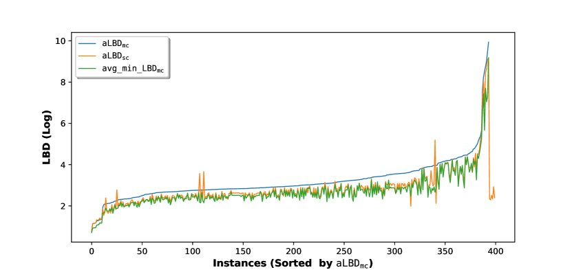
Figure 1: Clause Quality in Conflict Generating Decisions

Columns C and D in Table 1 compare LBD scores when averaged over sc and mc decisions. On average, sc decisions generate higher quality learned clauses (with lower LBD scores). However, Column E shows that in most cases, the minimum LBD score over the clauses in a single mc decision is lower on average than for sc. The exception is the UNSOLVED category. Fig. 1 shows per-instance details of these three measures in log scale. In almost all instances, LBD scores for mc (blue) are higher than for sc (orange), and minimum mc LBD (green) is lowest.

To summarize, on average mc decisions are conflict-inefficient compared to sc decisions. However, on average the best quality learned clause from a mc decision has better quality than the quality of a sc clause.

3.3 Bursts of mc Decisions

Column F in Table 1 shows the average value of avgBurst for the test set. On average, the burst of mc decisions are quite small, about 2.65. However, as shown in column G, the average value of maxBurst is very high. The left plot in Fig. 2 compares these values for each test instance in log scale. In almost all cases maxBurst (orange) is much larger than the average (blue). This indicates that while large bursts of mc decisions occur, they are rare, as indicated by the average of 2.65. To analyze this in detail, we count the number of mc decisions for each burst size from 2 to 10.

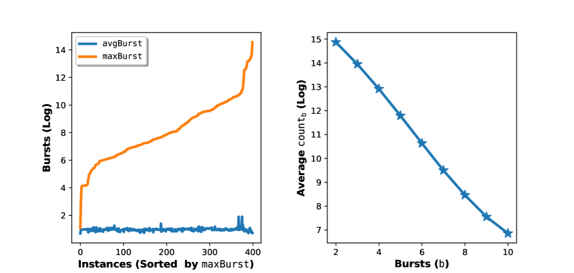
Figure 2: Analysis of Bursts of mc decisions

Distribution of mc Decisions by Burst Size Column G of Table 1 illustrates that maxBurst can be very large. To simplify our quantitative analysis we focus on counting mc decisions with bursts up to 10. The plot on the right of Fig. 2 shows the average (over the 400 instances in our test set) count (in log scale) of the number of bursts of a given size $b$, with $2\leq b\leq 10$. The frequency of bursts decreases exponentially with their size.

4 Clause Learning in mc Decisions

In this section, we establish a structural property of the learned clauses in mc decisions.

Formalization of mc Decisions Let $v$ be the decision variable for the mc decision $\mathcal{M}$ with burst $x\geq 2$. At the time when the search reaches the first conflict $C_{1}$ in $\mathcal{M}$, let $P_{0}$ be the set of literal assignments that follows from the assignment of $v$. With $1\leq i\leq x$, let $C_{i}$ be the $i^{th}$ conflicting clause, from which the clause $L_{i}=R_{i}\lor\{\lnot f_{i}\}$ is learned. Here, $R_{i}$ is the reason clause and $f_{i}$ is the fUIP literal for this $i^{th}$ conflict. After learning $L_{i}$, and after backtracking, $\lnot f_{i}$ is the only unassigned literal in $L_{i}$, and it is immediately unit-propagated from $L_{i}$. Let $P_{i}$ be the propagation block that contains literal assignments starting from the assignment of $\lnot f_{i}$ until the search reaches the conflicting clause $C_{i+1}$. Let $\mathcal{L}=(L_{1},\dots,L_{x})$ be the ordered sequence of $x$ learned clauses in $\mathcal{M}$.

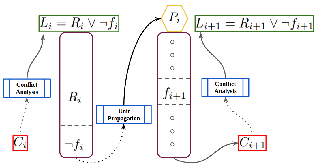
Figure 3: Connection between learned clauses in $\mathcal{M}$. After backtracking, $L_{i}$ forces $\lnot f_{i}$, the negated literal of the fUIP for the conflict at $C_{i}$. This forced assignment creates a block of assignment $P_{i}$, until the search reaches a conflict at $C_{i+1}$. $P_{i}$ contains $f_{i+1}$, which is the fUIP of the conflict at $C_{i+1}$. From $C_{i+1}$, Conflict Analysis learns $L_{i+1}$, which contains $\lnot f_{i+1}$.

Claim 1:

$\mathcal{M}$ learns a sequence of clauses $\mathcal{L}=(L_{1},\dots,L_{x})$, where a clause $L_{i}~{}(1\leq i<x)$ implicitly constructs $L_{i+1}$, by implying $f_{i+1}$, the fUIP literal for the $(i+1)^{th}$ conflict, from which $L_{i+1}$ is learned.

We justify Claim 1 as follows:

With $1\leq i<x$, after learning the $i^{th}$ clause $L_{i}=R_{i}\lor\lnot f_{i}$ and backtracking to a previous level, the literal $\lnot f_{i}$ (the negated literal of the fUIP of $i^{th}$ conflict) is forced in $L_{i}$. This forced assignment creates a propagation block $P_{i}$ and reaches the conflicting clause $C_{i+1}$. From $C_{i+1}$ the search learns the next clause $L_{i+1}=R_{i+1}\lor\lnot f_{i+1}$ within the current mc decision. Clearly, the fUIP of $i+1^{th}$ conflict, $f_{i+1}\in P_{i}$, as $\lnot f_{i+1}\in L_{i+1}$ is the only literal assigned in the current decision level. Fig. 3 shows the connection between $L_{i}$ and $L_{i+1}$.

We have $(a)(L_{i}=R_{i}\lor\lnot f_{i})\rightarrow f_{i+1},\;\;\;(b)f_{i+1}\in P_{i},\;\;\;\textnormal{and}\;\;(c)\lnot f_{i+1}\in L_{i+1}$

Hence, under the current partial assignment, the learning of $L_{i}$ is a sufficient condition for the learning of $L_{i+1}$. Any pair of consecutive clauses $(L_{i},L_{i+1})$ are connected via the pair of assignments $(\lnot f_{i},f_{i+1})$, where the first assignment in this pair is the negated literal of the fUIP literal for the $i^{th}$ conflict and the second assignment is the fUIP literal for the $(i+1)^{th}$ conflict.

Since the argument applies to all $1\leq i<x$, we have the desired result.

5 Proximity between Conflicts Sequences in CDCL

By Claim 1, we see that learned clauses in a mc decision are connected. This indicates that conflicts in a mc decision are also related, as clauses are learned from conflicts. Here, we first introduce the measure of ConflictsProximity to study proximity between conflict sequences and then present an empirical study to reveal insights on proximity between conflicts sequences in CDCL.

5.1 Conflicts Proximity

The notion of conflicts proximity uses a novel measure called Literal Block Proximity, which measures the commonality of literal blocks between a sequence of reason clauses over a sequence of conflicts.

5.1.1 Literal Block Proximity

Assume that from a conflicting clause $C$, $L=R\lor{\lnot f}$ is learned, where $R$ is the reason clause for the conflict at $C$ and $f$ is the fUIP literal of current conflict. We define a mapping

$$\mathcal{D}{}:\mathtt{Clause}\longmapsto\mathtt{\{dl_{1}\dots dl_{n}\}}$$

which maps a given reason clause $R$ to the set of distinct decision levels in $R$. Each $\mathtt{dl}\in\mathcal{D}{}(R)$ corresponds to the block of literals $\texttt{block}_{\mathtt{dl}}$ in $R$ which were assigned in $\mathtt{dl}$.

Let $\mathcal{R_{\mathcal{C}}}=(R_{1},\dots,R_{m})$ be the sequence of reason clauses for the conflicting clauses in $\mathcal{C}=(C_{1},\dots C_{m})$, where $R_{i}\in\mathcal{R}$ is the reason clause for the conflict at $C_{i}\in\mathcal{C}$. We define the set Literal Block Proximity (LBP) for $\mathcal{R}_{\mathcal{C}}$, $\mathbf{LBP_{\mathcal{R}_{\mathcal{C}}}}{}$ by

$$\mathbf{LBP_{\mathcal{R}_{\mathcal{C}}}}{}=\mathcal{D}{}(R_{1})\cap\dots\cap\mathcal{D}{}(R_{m})$$

That is, $\mathbf{LBP_{\mathcal{R}_{\mathcal{C}}}}{}$ is the set of decision levels that are common in all clauses in $\mathcal{R}$. Therefore, the assignments in $\mathtt{block_{dl}}$ with $\texttt{dl}\in\mathbf{LBP_{\mathcal{R}_{\mathcal{C}}}}{}$, contribute to the discovery of every conflicting clause in $\mathcal{C}$.

Example 1:

Let $\mathcal{R}_{\mathcal{C}}{}=(R_{a},R_{b})$ be a set of reason clauses for the conflicts at clauses in $\mathcal{C}=(C_{a},C_{b})$. Let $\mathcal{D}(R_{a})=$ {2, 9, 14, 35, 110} and $\mathcal{D}(R_{b})=$ {9, 10, 11, 35, 98, 110} be the sets of decision levels in $R_{a}$ and $R_{b}$, respectively. Then $\mathbf{LBP_{\mathcal{R}_{\mathcal{C}}}}{}=\mathcal{D}(R_{a})\cap\mathcal{D}(R_{b})$ = {9, 35, 110}. The assignments in $\texttt{block}_{9}$, $\texttt{block}_{35}$, and $\texttt{block}_{110}$ contribute to the generation of conflicts in both $C_{a}$ and $C_{b}$.

5.1.2 ConflictsProximity

For a reason clause sequence $\mathcal{R}_{\mathcal{C}}=(R_{1},\dots,R_{m})$, we define the ConflictsProximity $\mathtt{cp_{\mathcal{R}_{\mathcal{C}}}}{}$, with $0\leq\mathtt{cp_{\mathcal{R}_{\mathcal{C}}}}{}\leq 1$ as

$$\mathtt{cp_{\mathcal{R}_{\mathcal{C}}}}{}=\frac{|\mathbf{LBP_{\mathcal{R}_{\mathcal{C}}}}{}|}{|U_{\mathcal{R}_{\mathcal{C}}}|}$$

where $U_{\mathcal{R}_{\mathcal{C}}}=\mathcal{D}{}(R_{1})\cup\dots\cup\mathcal{D}{}(R_{m})$ is the set of all literal blocks in $\mathcal{R}_{\mathcal{C}}{}$. In Example 1, $\mathtt{cp_{\mathcal{R}_{\mathcal{C}}}}=\frac{|\mathbf{LBP_{\mathcal{R}_{\mathcal{C}}}}{}|}{|U_{\mathcal{R}_{\mathcal{C}}}|}=3/8$.

Intuitively, for any two given reason clause sequences $\mathcal{R}_{\mathcal{C}}{}_{p}$ and $\mathcal{R}_{\mathcal{C}}{}_{q}$, with $|\mathcal{R}_{\mathcal{C}}{}_{p}|=|\mathcal{R}_{\mathcal{C}}{}_{q}|$, if $\texttt{cp}_{\mathcal{R}_{\mathcal{C}}{}_{p}}>\texttt{cp}_{\mathcal{R}_{\mathcal{C}}{}_{q}}$, then the conflicts associated with the reason clauses in $\mathcal{R}_{\mathcal{C}}{}_{p}$ are more closely related to each other than conflicts associated with the reason clauses in $\mathcal{R}_{\mathcal{C}}{}_{q}$. If $\texttt{cp}_{\mathcal{R}_{\mathcal{C}}{}_{p}}>\texttt{cp}_{\mathcal{R}_{\mathcal{C}}{}_{q}}$, then we call the conflicts generated over the clauses in $\mathcal{C}_{p}$ more closely related than the conflicts generated over the clauses in $\mathcal{C}_{q}$.

Example 2:

Let $\mathcal{R}_{\mathcal{C}}{}_{p}=(R_{p1},R_{p2})$ and $\mathcal{R}_{\mathcal{C}}{}_{q}=(R_{q1},R_{q2})$ be two sequences of reason clauses for conflicts generated at the conflicting clauses in $\mathcal{C}_{p}=(C_{p1},C_{p2})$ and $\mathcal{C}_{q}=(C_{q1},C_{q2})$, respectively. Let $\texttt{cp}_{\mathcal{R}_{\mathcal{C}}{}_{p}}=0.65$ and $\texttt{cp}_{\mathcal{R}_{\mathcal{C}}{}_{q}}=0.35$. Then conflicts generated over the conflicting clauses in $\mathcal{C}_{p}$ are more closely related than conflicts generated over the conflicting clauses in $\mathcal{C}_{q}$.

We now study proximity of conflicts in CDCL under ConflictsProximity.

5.2 Proximity of Conflicts over sc and mc Decisions

While the learned clauses in a mc decision are connected, each learned clause in a sc decision is learned in isolation. Based on this observation, we propose the following hypothesis:

Hypothesis 1:

On average, conflicts in a mc decision with burst $x$ are more closely related than conflicts which are generated in the last $x$ sc decisions.

We support this hypothesis by comparing the ConflictsProximity of reason clauses over mc and sc decisions.

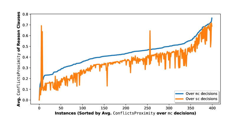
Figure 4: Comparison of average ConflictsProximity of Reason Clauses over mc and sc Decisions

Experiment We have performed an experiment with 400 instances from SAT20 with MplDL with a time-limit of 5,000 seconds. For each run of an instance, whenever the search finds a mc decision with burst $x$, we compute the LBP and ConflictsProximity for the reason clauses (i) for these $x$ conflicts and (ii) for the last $x$ conflicts in sc decisions. For this experiment, we collect data for bursts $x\leq 10$. For a run with an instance, we compute the average of ConflictsProximity of reason clauses separately over mc and sc decisions.

Fig. 4 shows that average ConflictsProximity for the reason clauses over mc decisions (blue lines, average is 0.43) are higher than ConflictsProximity of reason clauses over sc decisions (orange line, average is 0.34) for almost all instances. This validates our hypothesis that conflicts over mc decisions are more closely related than conflicts over sc decisions.

6 The Common Reason Variable Reduction Strategy

6.1 Common Reason Decision Variables

Assume that a mc decision $\mathcal{M}$ finds $x\geq 2$ consecutive conflicts within its decision. Let $\mathcal{R}=(R_{1},\dots,R_{x})$ be the sequence of reason clauses for these $x$ conflicts. $\mathbf{LBP_{\mathcal{R}}}$ is the set of common decision levels over $\mathcal{R}$. For each decision level $\mathtt{dl}\in\mathbf{LBP_{\mathcal{R}}}$, we call $\mathtt{dl}$, a common reason decision level and the decision variable $v$ at $\mathtt{dl}$, a common reason decision variable (CRV) for $\mathcal{M}$. If $|\mathbf{LBP_{\mathcal{R}}}|=z$, then there are $z$ CRVs in $\mathcal{M}$. The CRVs in $\mathcal{M}$ are the decision variables from previous decision levels, which contributed to the generation of all the conflicts in $\mathcal{M}$.

6.2 Poor mc Decisions

Recall that in Section 3 (Fig. 1), we observed that on average, mc decisions (blue line) produce lower quality clauses than sc decisions (orange line). However, the best quality clause (green line) in a mc decision has better average quality than other learned clauses. However, in a poor mc decision its best quality learned clause is worse than the average quality. A mc decision $\mathcal{M}$ is poor,

• if the quality of the best learned clause in $\mathcal{M}$ is lower than a dynamically computed threshold $\theta$, the average quality of the last $k$ learned clauses.

Table 2: The CRVR Decision Strategy

DetectPoorCRV	CRVRBranching
1. $\theta\leftarrow aLBD(k)$ 2. if ($\texttt{min\_LBD}_{\mathcal{M}}\;>\;\theta)$    a. $\mathcal{R}\leftarrow reason\_clauses\_in\_\mathcal{M}()$    b. for each $\mathtt{dl}\in\mathbf{LBP_{\mathcal{R}}}$       i. $\mathtt{v}\leftarrow dvar(\mathtt{dl})$       ii. poor_crv[v] $\leftarrow$ true	1. selected $\leftarrow$ false 2. while (not selected)     a. $\mathtt{y}\leftarrow$ select_next_free_var()     b. if (poor_crv[y])         i. activity[y] $\leftarrow$ activity[y] * (1-Q)         ii. poor_crv[y] $\leftarrow$ false         iii. reorder()      c. else          i. selected$\leftarrow$true

6.3 The CRVR Decision Strategy

We summarize the previous two subsections as follows:

• Conflicts in a poor mc decision are not likely to be helpful, as the quality of its best learned clause is lower than the recent search average.

• The CRVs in a poor mc decision combinedly contribute to the generation of these conflicts.

Does suppression of such CRVs for the future decisions help the search to achieve better efficiency? We address this question by designing a decision strategy named common reason variable score reduction (CRVR), which can be integrated with any activity based variable selection decision heuristics, such as VSIDS and LRB. The high-level idea of CRVR is as follows: Once a poor mc decision is detected, CRVR (i) finds the CRVs for that poor mc and (ii) marks those CRVs as poor CRVs, and (iii) then reduces the activity scores of those poor CRVs for future decisions. CRVR consists of the two procedures DetectPoorCRV and CRVRBranching, whose pseudo-codes are shown in Table 2.

DetectPoorCRV This procedure is invoked at the end of an mc decision $\mathcal{M}$ and just before the next decision. It computes a dynamic conflict quality threshold $\theta$, the average LBD score of last $k$ learned clauses. Then it determines if $\mathcal{M}$ is poor. by comparing min_LBD_Mwith $\theta$. In this case, DetectPoorCRV obtains the sequence of reason clauses $\mathcal{R}$ in $\mathcal{M}$ and computes $\mathbf{LBP_{\mathcal{R}}}$. For each decision level $\mathtt{dl}\in\mathbf{LBP_{\mathcal{R}}}$, any decision variable $\mathtt{v}$ at $\mathtt{dl}$ is marked as poor.

CRVRBranching is shown in the right side of Table 2. This procedure modifies a typical CDCL decision routine to lazily reduce the activity score of poor CRVs. It employs a while loop until a variable is selected, where in each iteration of the loop, it performs the following operations: (i) obtains a free variable y, where y is the free variable with largest activity score. (ii) checks if y is marked as poor. If y is poor, then it computes a fraction of activity[y], the current activity score of y, by multiplying it with (1-Q), where Q is a user defined parameter with $0<\mathtt{Q}<1$ . This fraction, which is lower than activity[y], becomes the new activity score of y. (iii) it unmarks y as poor and performs a reordering of the variables, which reorders the variables by their activity scores. The reduction of the activity score of y, followed by reordering, decreases the selection priority of y.

7 Experimental Evaluation

7.1 Implementation

We implemented CRVR in three state-of-the-art baseline solvers MplDL, Kissat-sat and Kissat-default. We call the extended solvers MplDL^crvr, Kissat-sat^crvr, and Kissat-default^crvr, respectively. The solver MplDL employs a combination of the decision heuristics DIST [29], VSIDS [22] and LRB [18], which are activated at different phases of the search, whereas Kissat-sat and Kissat-default use VSIDS and Variable Move to Front (VMTF) [26] alternately during the search.

The heuristics DIST, VSIDS and LRB share similar computational structures. All three heuristics maintain an activity score for each variable. Whenever a variable involves in a conflict, its activity score is increased. In contrast, VMTF maintains a queue of variables, where a subset of variables appearing in a learned clause are moved to the front of that queue in an arbitrary order.

CRVR is designed to be employed on top of activity-based decision heuristics. Hence in Kissat-sat^crvr and Kissat-default^crvr, we employ CRVR only when VSDIS is active.

In all of our extended solvers, we use the following parameter values: a length of window of recent conflicts $k=50$ and an activity score reduction factor Q $=0.1$. Source code of our CRVR extensions are available at [4].

Table 3: Comparison between 3 baselines and their CRVR extensions

Systems	SAT	UNSAT	Combinded	PAR-2
MplDL	106	110	216	2065
MplDLcrvr	116 (+10)	107 (-3)	223 (+7)	2001
Kissat-sat	148	118	266	1552
Kissat-satcrvr	150 (+2)	114 (-4)	264 (-2)	1565
Kissat-default	134	126	260	1624
Kissat-defaultcrvr	139 (+5)	125 (-1)	264 (+4)	1588

7.2 Experiments and Results

We conduct experiments with the same set of 400 instances with a 5,000 seconds timeout per instance. We compare the CRVR extensions and their counterpart baselines in terms of number of solved instances, solving time and PAR-2 score.

Table 3 compares MplDL^crvr, Kissat-sat^crvr, and Kissat-default^crvr with their baselines. All of these extensions show performance gains on SAT instances, but lose on UNSAT instances. The strongest gain is for MplDL^crvr, which solves 10 additional SAT instances, but solves 3 less UNSAT instances, achieves an overall gain of 7 instances compared to its baseline. Kissat-sat^crvr solves 2 more SAT instances, but looses 4 UNSAT instances, with an overall loss of 2 instances compared to its baseline. The third extension Kissat-default solves 5 more SAT instances, but solves 1 less UNSAT instance than its baseline. Overall, Kissat-default^crvr solves 4 more instances than Kissat-default.

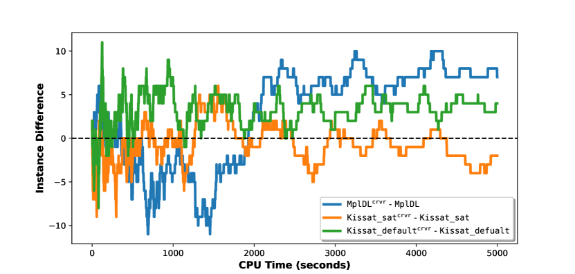
Figure 5: Solve time comparisons: For any point above 0 in the vertical axis, our extensions solve more instances than their baselines at the time point in the horizontal axis.

The PAR-2 results are consistent with the solution count results. While Kissat-sat^crvr has a slight increase (a 0.8% increase) in its PAR-2 score compared to Kissat-sat, both MplDL^crvr and Kissat-default^crvr have significantly lower PAR-2 scores (3.19% and 2.28% of reductions, respectively) compared to their baselines, which reflects overall better performance of these two systems compared to their baselines.

Fig. 5 compares the relative solving speed of MplDL^crvr (blue), Kissat-sat^crvr (orange), and Kissat-default^crvr (green) against their baselines by plotting the difference in the number of instances solved as a function of time. If that difference is above 0, then it indicates that an extended solver solves more instances than the baseline at this time point.

MplDL^crvr (blue) performs slightly worse than MplDL early on, but beats the baseline consistently after 1,900 seconds. Compared to Kissat-default, Kissat-default^crvr (green) is ahead of Kissat-default at most time-points. Kissat-sat^crvr (orange) is behind Kissat-sat at most of the time-points.

Overall, compared to their baselines, our extensions perform better on SAT instances, but loose a small number of UNSAT instances.

8 Detailed Performance Analysis of CRVR

For a run of a given solver, the metric GLR measures the overall conflict generation rate of the search, average LBD (aLBD) measures the average quality of the learned clauses and G2L measures the fraction of learned clauses which are glue. All these measures correlate well with solving efficiency [10, 19]. Here, we present an analysis that relates the performance of CRVR with these three metrics. We consider two subsets of instances, where MplDL and MplDL^crvr show opposite strengths:

• $\mathtt{CRVR\!\!-\!\!bad}$: 12 instances which are solved by MplDL, but not by MplDL^crvr.

• $\mathtt{CRVR\!\!-\!\!good}{}$: 19 instances which are solved by MplDL^crvr, but not by MplDL.

Table 4: Relating solving efficiency with three metrics average GLR, average LBD and average G2L. More efficient branching heuristics tend to achieve higher average GLR [19], higher average G2L [10] and lower average aLBD [19] than less efficient ones.

Instance Sets	Count (SAT+UNSAT)	average GLR		average aLBD		average G2L
		MplDL	MplDLcrvr	MplDL	MplDLcrvr	MplDL	MplDLcrvr
$\mathtt{CRVR\!\!-\!\!good}{}$	19 (18+1)	0.58	53	4399.91	147.69	0.003	0.018
$\mathtt{CRVR\!\!-\!\!bad}{}$	12 (8+4)	0.56	0.56	18.83	18.53	0.024	0.023

The 19 instances in $\mathtt{CRVR\!\!-\!\!good}{}$ (first row of Table 4) are solved exclusively by MplDL^crvr. For this subset, MplDL^crvr learns clauses at a slightly lower rate. However, for $\mathtt{CRVR\!\!-\!\!good}{}$, the average aLBD (resp. average G2L) is significantly lower (resp. higher) with MplDL^crvr. CRVR helps to (i) learn higher quality clauses, and (ii) learn more glue clauses relative to the number of clauses for the subset of instances in $\mathtt{CRVR\!\!-\!\!good}{}$, for which MplDL^crvr is efficient.

18 of the 19 instances in $\mathtt{CRVR\!\!-\!\!good}{}$ are SAT. The learning of significantly better quality of clauses with MplDL^crvr for these SAT instances may just explain the good performance of CRVR on SAT instances.

For the 12 instances in $\mathtt{CRVR\!\!-\!\!bad}{}$ (second row of Table 4), MplDL learns clauses at the same rate, but learns clauses which are of slightly lower quality than the clauses learned by MplDL^crvr. However, for this set, the average G2L value is slightly higher with MplDL than MplDL^crvr. This could explain the better performance of MplDL for this subset.

9 Related Work

Audemard and Simon [5] briefly studied decisions with successive conflicts, which we refer to as mc decisions in this paper. They studied number of successive conflicts in the CDCL solver Glucose on a fixed set of instances. In the current paper, we present a more formal and in-depth study of mc decisions. The authors of [19] relate conflict generation propensity and learned clause quality with the efficiency of several decision heuristics. In contrast, we study and compare the conflict quality of two types of conflict producing decisions for CDCL. Conflicts generation pattern in CDCL is studied in [9] showing that CDCL typically alternates between bursts and depression phases of conflict generation. While that work presented an in-depth study of the conflict depression phases in CDCL, here we study the the conflict bursts phases, which are opposite of conflict depression phases. Chowdhury et al. [10] studied conflict efficiency of decisions with two types of variables: those that appear in the glue clauses and those that do not. In the current paper, we compare the conflict efficiency of conflict producing decisions.

10 Conclusions and Future Work

We present a characterization of sc and mc decisions in terms of average learned clause quality that each type produces. Then we analyze how mc decisions with different bursts are distributed in CDCL search. Our theoretical analysis shows that learned clauses in a mc are connected, indicating that conflicts that occur in a mc decision are related to each other. We introduced a measure named ConflictsProximity that enables the study of proximity of conflicts in a given sequence of conflicts. Our empirical analysis shows that conflicts in mc decisions are more closely related than conflicts in sc decisions. Finally, we formulated a novel CDCL strategy CRVR that reduces the activity score of some variables that appear in the clauses learned over mc decisions. Our empirical evaluation with three modern CDCL SAT solvers shows the effectiveness of CRVR for the SAT instances from SAT20.

In the future, we intend to pursue the following research questions:

• Kissat solvers and their predecessors, such as CaDiCaL, employ VMTF as one of their decision heuristics. How to extend VMTF with CRVR is an interesting question that we plan to pursue in future.

• Currently, the user defined parameters $k$ and Q in CRVR are set to fixed values. How to adapt them dynamically during the search? We hope that a dynamic strategy to adapt these parameters will improve the performance of CRVR, specially over the UNSAT instances.

References

- [1] SAT Competition 2020, http://sat2018.forsyte.tuwien.ac.at/index-2.html, accessed date: 2021-03-06.
- [2] SAT Competition 2020, https://satcompetition.github.io/2020/downloads.html, accessed date: 2021-03-06.
- [3] SAT race 2019, http://sat-race-2019.ciirc.cvut.cz/solvers/, accessed date: 2021-03-10.
- [4] CRVR Extensions of 3 CDCL Solvers: Source Code, https://figshare.com/articles/software/CRVR_Extensions/14229065, accessed date: 2021-03-17.
- [5] Gilles Audemard and Laurent Simon. Extreme cases in SAT problems. In Proceedings of SAT 2016, pages 87–103.
- [6] Gilles Audemard and Laurent Simon. Predicting learnt clauses quality in modern SAT solvers. In Proceedings of IJCAI 2009, pages 399–404, 2009.
- [7] Gilles Audemard and Laurent Simon. Refining restarts strategies for SAT and UNSAT. In Proceedings of CP 2012, pages 118–126, 2012.
- [8] Cristian Cadar, Vijay Ganesh, Peter M. Pawlowski, David L. Dill, and Dawson R. Engler. EXE: automatically generating inputs of death. In Proceedings of CCS 2006, pages 322–335, 2006.
- [9] Md. Solimul Chowdhury, Martin Müller, and Jia You. Guiding CDCL SAT search via random exploration amid conflict depression. In Proceedings of AAAI 2020, pages 1428–1435, 2020.
- [10] Md. Solimul Chowdhury, Martin Müller, and Jia-Huai You. Exploiting glue clauses to design effective CDCL branching heuristics. In CP 2019, pages 126–143.
- [11] Stephen A. Cook. The complexity of theorem-proving procedures. In Proceedings of the 3rd Annual ACM Symposium on Theory of Computing, pages 151–158, 1971.
- [12] Martin Davis, George Logemann, and Donald W. Loveland. A machine program for theorem-proving. Commun. ACM, 5(7):394–397, 1962.
- [13] Niklas Eén and Armin Biere. Effective preprocessing in SAT through variable and clause elimination. In Proceedings of SAT 2005, pages 61–75, 2005.
- [14] Aarti Gupta, Malay K. Ganai, and Chao Wang. SAT-based verification methods and applications in hardware verification. In Proceedings of SFM 2006, pages 108–143, 2006.
- [15] Matti Järvisalo, Armin Biere, and Marijn Heule. Blocked clause elimination. In Proceedings of TACAS 2010, pages 129–144, 2010.
- [16] Matti Järvisalo, Marijn Heule, and Armin Biere. Inprocessing rules. In Proceedings of IJCAR 2012, pages 355–370, 2012.
- [17] Jia Hui Liang, Vijay Ganesh, Pascal Poupart, and Krzysztof Czarnecki. Exponential recency weighted average branching heuristic for SAT solvers. In Proceedings of AAAI 2016, pages 3434–3440, 2016.
- [18] Jia Hui Liang, Vijay Ganesh, Pascal Poupart, and Krzysztof Czarnecki. Learning rate based branching heuristic for SAT solvers. In Proceedings of SAT 2016, pages 123–140, 2016.
- [19] Jia Hui Liang, Hari Govind, Pascal Poupart, Krzysztof Czarnecki, and Vijay Ganesh. An empirical study of branching heuristics through the lens of global learning rate. In Proceedings of SAT 2017, pages 119–135, 2017.
- [20] Mao Luo, Chu-Min Li, Fan Xiao, Felip Manyá, and Zhipeng Lü. An effective learnt clause minimization approach for CDCL SAT solvers. In Proceedings of the Twenty-Sixth International Joint Conference on Artificial Intelligence, IJCAI-17, pages 703–711, 2017.
- [21] Fabio Massacci and Laura Marraro. Logical cryptanalysis as a SAT problem. J. Autom. Reasoning, 24(1/2):165–203, 2000.
- [22] Matthew W. Moskewicz, Conor F. Madigan, Ying Zhao, Lintao Zhang, and Sharad Malik. Chaff: Engineering an efficient SAT solver. In Proceedings of DAC 2001, pages 530–535, 2001.
- [23] Alexander Nadel and Vadim Ryvchin. Chronological backtracking. In Proceedings of SAT 2018, pages 111–121, 2018.
- [24] Chanseok Oh. Between SAT and UNSAT: the fundamental difference in CDCL SAT. In Proceedings of SAT 2015, pages 307–323, 2015.
- [25] Jussi Rintanen. Engineering efficient planners with SAT. In Proceedings of ECAI 2012, pages 684–689, 2012.
- [26] Lawrence Ryan. Efficient algorithms for clause-learning SAT solvers. Master’s thesis, Simon Fraser University, 2004.
- [27] João P. Marques Silva and Karem A. Sakallah. GRASP: A search algorithm for propositional satisfiability. IEEE Trans. Computers, 48(5):506–521, 1999.
- [28] Mate Soos, Karsten Nohl, and Claude Castelluccia. Extending SAT solvers to cryptographic problems. In Proceedings of SAT 2009, pages 244–257, 2009.
- [29] Fan Xiao, Mao Luo, Chu-Min Li, Felip Manyá, and Zhipeng Lu. MapleLRB_LCM, Maple_LCM, Maple_LCM_Dist, MapleLRB_LCMoccRestart and Glucose3.0+width in SAT competition 2017. In Proceedings of SAT Competition 2017, pages 22–23, 2017.