Policy Synthesis for Metric Interval Temporal Logic with Probabilistic Distributions

Abstract

Metric Temporal Logic can express temporally evolving properties with time-critical constraints or time-triggered constraints for real-time systems. This paper extends the Metric Interval Temporal Logic with a distribution eventuality operator to express time-sensitive missions for a system interacting with a dynamic, probabilistic environment. This formalism enables us to describe the probabilistic occurrences of random external events as part of the task specification and event-triggered temporal constraints for the intended system’s behavior. The main contributions of this paper are two folds: First, we propose a procedure to translate a specification into a stochastic timed automaton. Second, we develop an approximate-optimal probabilistic planning problem for synthesizing the control policy that maximizes the probability for the planning agent to achieve the task, provided that the external events satisfy the specification. The planning algorithm employs a truncation in the clocks for the timed automaton to reduce the planning in a countably infinite state space to a finite state space with a bounded error guarantee. We illustrate the method with a robot motion planning example.

I Introduction

This paper investigates a probabilistic planning problem given a time-sensitive task expressed in Metric Interval Temporal Logic with distributions. The task specifies the assumption about the probabilistic external events and the desired agent’s behavior with timing constraints related to the occurrence of the external events. Such problem is widely encountered in robotics [1, 2], and other cyber-physical systems [3].

Temporal Logic is a formal language to describe desired system properties, such as safety, reachability, obligation, stability, and liveness [4]. Recently, Metric Temporal Logic (MTL) [5], Metric Interval Temporal Logic (MITL) [6](a fragment of MTL), and Signal Temporal Logic (STL) [7] have received extensive attention in the control community, due to their capability of not only expressing the relative temporal ordering of events as Linear Temporal Logic (LTL) [8] but also defining the duration and timing constraints between these events and robustness of controlled systems. Given high-level specifications, the control synthesis for dynamic systems have been developed for linear systems [9, 10] and linear systems subject to nondeterministic inputs from the environment [11, 12], multi-agent systems [13, 14], Markov Decision Processes (MDPs) [15], and Mixed Logical Dynamical systems [16]. Mixed integer linear programming has been introduced for robust planning and control in discrete-time, linear systems [11, 12] and Mixed Logical Dynamical Systems [16], where the STL formula was translated to a set of constraints in the optimization problem. Recent work [10] utilized the Control Barrier Function to plan trajectories that satisfy the STL specifications. In particular, they utilized the lower bound of a Control Barrier Function to make the constraint on the always temporal operator to be time-invariant. In [16], authors considered specifications expressed in MTL for a Mixed Logical Dynamical System. The synthesis of provably correct timed systems has been investigated in the formal methods community using automata-theoretic approaches. The authors in [17] investigated a control synthesis problem for a timed system, and the specification was captured by an external timed automaton. They modeled the dynamic interaction between the timed system and the environment as a timed game, where the clocks in the timed automaton were assumed to be upper bounded. The authors [18] studied multi-agent control with intermittent communication. They solved the problem by developing a leader-follower formulation while the leader must satisfy a MITL formula.

Existing works assume that temporal logic specifications only describe the intended system’s behavior where the environment is either static [18, 10] or nondeterministic [17, 11, 12]. However, in practical applications, an event in the environment may follow a probability distribution. To illustrate, consider that an autonomous robot is working in a remote area and must catch a bus when a bus arrives. The robot is equipped with the knowledge that the bus’s arrival (event) follows a probability distribution. An autonomous car, stopped at a red light, may have a probability distribution of how long to wait for the light to turn green. A patrolling robot may need to interdict illegal fishing, have prior knowledge about when the illegal activities may occur at different sites, and must respond to each detected activity within a bounded time duration. How do we incorporate this knowledge into the specification and how to synthesize a policy that maximizes the probability of satisfying such a time-sensitive task?

Our approach follows from assume-guarantee reasoning: We adopt the MITL to describe the intended system’s behavior (guarantee). To capture the assumption of the environment, we consider a new class of distributional temporal logic, proposed recently in [19]. In this logic language, an operator, called “distribution eventuality” $\leavevmode\hbox to5.38pt{\vbox to9.02pt{\text{[drawing]}}}_{\mu}\varphi$, is introduced to specify that the first time when $\varphi$ evaluated true follows the distribution $\mu\colon[0,\infty)\to[0,1]$. We augment MITL with the distribution eventuality operators, called Metric Interval Temporal Logic with Probabilistic Distributions (MITLD), to specify the intended behavior of the system and the model of its environment jointly. To this end, we propose a procedure to first translate the MITLD formula to a stochastic timed automaton, which is a finite-state automaton augmented with a set of clocks to keep track of time-dependent constraints. Given the interaction between the agent and its environment modeled as a two-player game, we introduce a product operation between the game and the stochastic timed automaton in order to restrict the external events in the environment to satisfy the pre-defined distributions. This product operation reduces the game into a countably infinite Markov Decision Process (MDP) with a reachability objective. We introduce a truncation in clocks to reduce the product MDP with countably infinite states into one with finite states and ensure the solution found in the latter is at least $\epsilon$-optimal for the original product MDP, where the $\epsilon$ is dependent on the truncation points. We use a running example to demonstrate our proposed method and provide discussions for future work.

II Preliminaries

Notation

We use the notation $\Sigma$ for a finite set of symbols, also known as the alphabet. An infinite sequence of symbols $\sigma=\sigma_{0}\sigma_{1}\ldots\ldots$ with $\sigma_{i}\in\Sigma$ for all $i\geq 0$, is called an infinite word, and $\Sigma^{\omega}$ is the set of all infinite words that are obtained by concatenating the elements in alphabet $\Sigma$ infinitely many times. Given a random variable $X$, we let $\mbox{Dist}(X)$ be the set of all possible probability distributions over $X$.

We consider a probabilistic planning problem for a controllable agent, referred to as a robot. The robot aims to satisfy a task specification in an uncertain, stochastic environment. Specifically, we consider the specification of the robot’s intended behavior and the environment’s behavior is expressed in a class of Metric Interval Temporal Logic with Probability Distributions (MITLD).

II-A Metric Interval Temporal Logic with Probability Distributions

The MITLD extends MITL [6] with a new operator $\leavevmode\hbox to5.38pt{\vbox to9.02pt{\text{[drawing]}}}_{\mu}\varphi$, called distribution eventuality [19] that expresses that the time until $\varphi$ evaluated true has a probability distribution $\mu$. Formally, MITLD formulas are built on MITL formulas and defined inductively as follows.

$$\varphi\coloneqq\top\mid p\mid\neg\varphi\mid\varphi\lor\varphi\mid\varphi\mbox{$\,{\sf U}$}_{I}\varphi\mid\varphi\mbox{$\,{\sf U}$}\varphi\mid\leavevmode\hbox to5.38pt{\vbox to9.02pt{\text{[drawing]}}}_{\mu}\varphi,$$

where $p\in\mathcal{AP}$, $\mu$ is a probability distribution, $\top$ is unconditional true, and $I$ is a nonsingular time interval with integer end-points. We also define temporal operator $\Diamond\,\varphi=\top\mbox{$\,{\sf U}$}\varphi$ (eventually, $\varphi$ evaluates true in the future) and $\Diamond\,_{I}\varphi=\top\mbox{$\,{\sf U}$}_{I}\varphi$ (eventually, $\varphi$ evaluates true within interval $I$ from now). The semantics of MITL and the distribution eventuality can be found in [6, 19] and omitted.

Note that we do not allow the distribution eventuality operator $\leavevmode\hbox to5.38pt{\vbox to9.02pt{\text{[drawing]}}}_{\mu}$ to appear in the scope of any negation since $\neg\leavevmode\hbox to5.38pt{\vbox to9.02pt{\text{[drawing]}}}_{\mu}\varphi$ simply says that the time until $\varphi$ evaluated true has a distribution different from $\mu$, which is an uninformative statement. When the context is clear, we may omit the subscript $\mu$ from these formulas.

This distribution eventuality is introduced by [19] for Linear Temporal Logic formulas. We extend it to use with Metric Interval Temporal Logic and also restrict it to a subclass of MITLD formulas, termed as MITLD^- , that satisfy the following conditions: 1) The formula has countably many MITL interpretations with discrete-time semantics. 2) There exists a subset $U\subset\mathcal{AP}$ of atomic propositions called “external events” such that the distribution eventuality operator can only occur in the front of a proposition in $U$. 3) If we replace the distribution eventuality operator with eventuality operator, the resulting formula is an MITL formula that can be equivalently expressed by a deterministic timed automaton, introduced later.

We provide some preliminary about timed words and timed automata.

A (infinite) timed word [20] over $\Sigma$ is a pair $w=(\tau,\sigma)$, where $\tau=\tau_{0}\tau_{1}\ldots$ is an infinite timed sequence and $\sigma=\sigma_{0}\sigma_{1}\ldots\in\Sigma^{\omega}$ is an infinite word. The infinite timed sequence $\tau=\tau_{0}\tau_{1}\ldots$ satisfies:

• Initialization: $\tau_{0}=0$;

• Monotonicity: $\tau$ increases strictly monotonically; i.e., $\tau_{i}<\tau_{i+1}$, for all $i\geq 0$;

• Progress: For every $t\in\mathbf{R}$, there exists some $i\geq 1$, such that $\tau_{i}>t$.

The conditions ensure that there are finitely many symbols (events) in a bounded time interval, known as non-Zenoness. We also write $w=(\tau,\sigma)=(\tau_{0},\sigma_{0})(\tau_{1},\sigma_{1})\ldots$.

A fragment of MITL that can be translated into an equivalent Deterministic Timed Automaton (DTA) [6]. To define timed automata, a finite number of clock and clock constraints are needed: Let $\operatorname{X}=\{\operatorname{x}_{1},\operatorname{x}_{2},\ldots,\operatorname{x}_{M}\}$ be a finite indexed set of clocks. For each clock $\operatorname{x}_{i}\in\operatorname{X}$, we let $\mathcal{V}_{i}$ be the range of that clock. A clock vector [21] $v\in\mathcal{V}_{i}$ is the vector where the $i$-th entry $v[i]$ is the value of clock $\operatorname{x}_{i}$, for $i\in\{1,2,\ldots,M\}$. We use $\mathbf{0}$ for the clock vector $v$ where $v[i]=0$ for all $i\in\{1,2,\ldots,M\}$ and $\mathcal{V}=\mathcal{V}_{1}\times\ldots\times\mathcal{V}_{M}$ for the set of all possible clock vectors. For a clock vector $v\in\mathcal{V}$ and $t\geq 0$, $v+t$ defines a clock vector $(v+t)[i]=v[i]+t$ for $i\in\{1,2,\ldots,M\}$. Moreover, if $Z\subseteq\operatorname{X}$ is a subset of clocks and $v$ is a clock vector, $v_{[Z\leftarrow 0]}$ denotes the clock vector after resetting the clocks in $Z$, such that $v_{[Z\leftarrow 0]}[i]=v[i]$ for all $\operatorname{x}_{i}\in\operatorname{X}\setminus Z$ and $v_{[Z\leftarrow 0]}[i]=0$ for all $\operatorname{x}_{i}\in Z$.

Definition 1 (Clock Constraints [20]).

For a set $\operatorname{X}$ of clocks, the set $\mathcal{C}(\operatorname{X})$ of clock constraints is defined inductively as follows:

$$c\coloneqq\perp\mid\operatorname{x}\bowtie k\mid\operatorname{x}-\operatorname{x}^{\prime}\bowtie k\mid c\land c\mid c\lor c,$$

where $\operatorname{x},\operatorname{x}^{\prime}\in\operatorname{X}$ are clocks, $k\in\mathbb{N}$ is a non-negative integer, and $\bowtie\in\{=,\neq,<,>,\geq,\leq\}$ is a comparison operator.

Given a clock constraint $c$ over $\operatorname{X}$ and a clock vector $v$, we write $v\models c$ whenever $v$ satisfies the constraints expressed by $c$.

Let us recall the definition of the deterministic timed automaton that accepts an MITL formula $\varphi^{d}$. The translation from a MITL formula to a DTA is introduced in [6, 22].

Definition 2 (Deterministic Timed Automaton).

A Deterministic Timed Automaton associated with an MITL formula $\varphi^{d}$ is a tuple $\operatorname{\mathcal{A}}=\langle L,\Sigma,\mathsf{Init},E,\operatorname{\mathcal{I}},F\rangle$ with the following components:

• $L$ is a finite set of locations.

• $\Sigma=2^{\mathcal{AP}}$ is a set of symbols.

• $\mathsf{Init}$ is an initial location.

• $E\colon L\times\Sigma\times\mathcal{C}(\operatorname{X})\times L\times 2^{\operatorname{X}}$ is a finite set of labeled edges.

• $\operatorname{\mathcal{I}}\colon L\to\mathcal{C}(\operatorname{X})$ assigns an invariant (clock constraint) to each location.

• $F\subseteq L$ is the set of accepting locations.

A state in the timed automaton is $(\ell,v)$ consisting of a pair of location and clock vector. The initial state in the timed automaton is $(\mathsf{Init},\mathbf{0})$. The transition $(\ell,v)\xrightarrow[\tau]{\sigma}(\ell^{\prime},v^{\prime})$ occurs only if there exists a symbol $\sigma\in\Sigma$, a constraint $c\in\mathcal{C}(\operatorname{X})$, and $\operatorname{X}^{\prime}\subseteq\operatorname{X}$ such that $e=(\ell,\sigma,c,\ell^{\prime},\operatorname{X}^{\prime})$ is defined, and for every $0\leq t<\tau$, $v+t\models\operatorname{\mathcal{I}}(\ell)$, and $v+\tau\models c$. Let $v^{\prime}=(v+\tau)_{[\operatorname{X}^{\prime}\leftarrow 0]}$ and $v^{\prime}\models\operatorname{\mathcal{I}}(\ell^{\prime})$. Intuitively, the timed automaton reads the input and also checks if the clock constraint of the edge is satisfied given the clock vector. If yes, then the transition occurs and a subset of clocks will be reset to zeros. After transition, the new clock vector should satisfy the invariant condition at the new location.

By the definition of transition, a run $\rho$ in $\operatorname{\mathcal{A}}$ on a timed word $w=(\tau_{0},\sigma_{0})(\tau_{1},\sigma_{1})\ldots$ is an infinite sequence of transitions $\rho=(\mathsf{Init},\mathbf{0})\xrightarrow[\tau_{0}]{\sigma_{0}}(\ell_{1},v_{1})\xrightarrow[\tau_{1}-\tau_{0}]{\sigma_{1}}\ldots(\ell_{i},v_{i})\xrightarrow[\tau_{i+1}-\tau_{i}]{\sigma_{i+1}}(\ell_{i+1},v_{i+1})\ldots$. The word $w=(\tau,\sigma)$ is accepted by the DTA if and only if its run reaches an accepting location in $F$; that is, $\mathsf{Occ}(\rho)\cap(F\times\mathcal{V})\neq\emptyset$, where $\mathsf{Occ}(\rho)$ is the set of states in $L\times\mathcal{V}$ occurring in $\rho$. The set of timed words accepted by $\operatorname{\mathcal{A}}$ is called its language, denoted as $\mathcal{L}(\operatorname{\mathcal{A}})$.

III Problem formulation

Recall that $U\subseteq\mathcal{AP}$ is the set of atomic propositions such that for each $\alpha\in U$, $\leavevmode\hbox to5.38pt{\vbox to9.02pt{\text{[drawing]}}}_{\mu_{\alpha}}\alpha$ is a subformula of the task specification $\varphi$. We assume that the agent’s action cannot change the values of propositions in $U$. The environment player controls the values of atomic propositions in $U$, and for any $\alpha\in U$, it only evaluates true only once. During the interaction, the agent will select an action, and the environment will select a subset of external events, and the next state is reached probabilistically according to a transition function.

This interaction between agent and its dynamic world can be captured by a two-player turn-based probabilistic transition system. The factored state means that a state $s\in S$ is a vector $s=[s_{r},s_{e},Y]^{\intercal}$ of robot state $s_{r}\in S_{r}$, environment state $s_{e}\in S_{e}$, and a set $Y\subseteq U$ that is a set of external events have not occurred yet. The set $S=S_{r}\times S_{e}\times 2^{U}$ is a finite set of possible states reachable given the interaction.

Definition 3.

The interaction between the robot and its environment is modeled as a two-player probabilistic transition system that is a tuple

$$\mathcal{G}=\langle S\cup S\times A,A\cup 2^{U},P,\operatorname{\mathsf{L}},s_{0},\mathcal{AP}\rangle$$

with the following components:

• $S\cup S\times A$ is a set of states partitioned into $S$ and $S\times A$. At each state in $S$, the robot takes an action, and at each state in $S\times A$, the environment takes an action.

• $A$ is the set of robot actions. $2^{U}$ is a set of environment actions.

• At each state in $S$, $P\colon S\times A\to S\times A$ is the deterministic transition function; that is, at a state $s\in S$, given the robot action $a\in A$, the transition to the next state $(s,a)$ is with probability $P(s,a,(s,a))=1$. At each state in $S\times A$, $P\colon S\times A\times 2^{U}\to\mbox{Dist}(S)$ is the probabilistic transition function; that is, at a state $(s,a)\in S\times A$, let $s=(s_{r},s_{e},Y)$, the environment player selects an enabled action $e\in 2^{Y}$, and $P((s,a),e,s^{\prime})$ is the probability of reaching state $s^{\prime}$ given the robot action $a$ from state $s$ and the environment action $e$. In addition, the state $s^{\prime}=(s_{r}^{\prime},s_{e}^{\prime},Y^{\prime})$ in the support of $P((s,a),e)$ must satisfy $Y^{\prime}=Y\setminus e$.

  In other words, the environment can only select a subset of events that have not occurred yet. Given the choice of the external events, the state will be updated to record the occurred events.

• $\operatorname{\mathsf{L}}\colon S\to 2^{\mathcal{AP}}$ is the labeling function such that $\operatorname{\mathsf{L}}(s)$ is a set of atomic propositions evaluated true at that state. For any $s$ that is reachable with the environment action $e$ with a nonzero probability; that is, $P((s,a),e,s^{\prime})>0$, the labeling must satisfies $\operatorname{\mathsf{L}}(s^{\prime})\cap U=e$.

• $s_{0}$ is an initial state.

In this game model, the two players can make nondeterministic choices of actions. The labeling of states captures which events in $U$ have occurred in the most recent transition.

We informally state the problem to be solved.

Problem 1.

Given the game model $\mathcal{G}$ and a task formula $\varphi=\varphi_{A}\land\varphi_{G}$ where $\varphi_{G}$ is the intended robot’s behavior in MITL and $\varphi_{A}$ is the assumption about the environment dynamics expressed in a MITLD^- formula, how to synthesize a control policy for the robot that maximizes the probability of satisfying the task formula?

IV Main Results

In this section, we present our solution to the planning problem.

IV-A Translating MITLD^- formulas to Stochastic Timed Automata

We first construct a computational model that represents the given task formula $\varphi$ in MITLD^- . To do so, we first substitute the distribution eventuality operators with the bounded eventuality operators $\Diamond\,_{\geq 0}$. This substitution will allow us to obtain an MITL formula $\varphi^{d}$ and its corresponding DTA $\operatorname{\mathcal{A}}$ using the construction from [6, 22]. After the substitution, we modify transitions to construct a corresponding Stochastic Timed Automaton (STA) for the original formula with distribution eventuality operators. The following assumption is made about the external events.

Assumption 1.

The set of random variables $\{\alpha\mid\alpha\in U\}$ are mutually independent.

Recall that the time until the formula $\alpha$ is first observed has a distribution $\mu_{\alpha}\colon[0,\infty)\to[0,1]$. Next, we introduce a stochastic timed automaton to represents the MITLD^- formula $\varphi$.

Definition 4 (Stochastic Timed Automaton).

Given an MITL formula $\varphi^{d}$ with the corresponding DTA $\operatorname{\mathcal{A}}=\langle L,\Sigma,\mathsf{Init},E,\operatorname{\mathcal{I}},F\rangle$, the STA that represents the distributions of MITL formulas expressed by the MITLD^- formula $\varphi$ is a tuple $\operatorname{\mathcal{S}}=\langle L,\Sigma,\mathsf{Init},\Delta,\operatorname{\mathcal{I}},F\rangle$ with the following components:

• $L,\Sigma,\mathsf{Init},\operatorname{\mathcal{I}},F$ are the same as in the DTA $\operatorname{\mathcal{A}}$ for $\varphi^{d}$.

• $\Delta\colon L\times\mathcal{V}\times 2^{U}\times(\Sigma\times\mathcal{C}(\operatorname{X}))\times(L\times\mathcal{V}\times 2^{\operatorname{X}}\times 2^{U})\to[0,1]$ is a probabilistic transition function, constructed as follows.

A state in the stochastic time automaton $\operatorname{\mathcal{S}}$ is $(\ell,v,Y)$ which includes a location, a clock vector, and an additional set of external events. The transition $(\ell,v,Y)\xrightarrow[\tau]{\sigma,p}(\ell^{\prime},v^{\prime},Y^{\prime})$ occurs with a probability $p>0$ only if $e=(\ell,\sigma,c,\ell^{\prime},\operatorname{X}^{\prime})\in E$ is defined in the DTA, $Y^{\prime}=Y\setminus\sigma$, and for every $0\leq t<\tau$, $v+t\models\operatorname{\mathcal{I}}(\ell)$, $v+\tau\models c$, $v^{\prime}=(v+\tau)_{[\operatorname{X}^{\prime}\leftarrow 0]}$, and $v^{\prime}\models\operatorname{\mathcal{I}}(\ell^{\prime})$. In addition, the clocks for occurred events, i.e., propositions in $U\setminus Y^{\prime}$, will be reset and stopped. To define probability $p$ of this transition, we distinguish four cases:

Case 1: if $Y=\emptyset$, then $p=1$. This is the case when all external events has occurred.

Case 2: if $Y\neq\emptyset$ and $\sigma\cap Y\neq\emptyset$ and $Y\setminus\sigma\neq\emptyset$, then

$$p=\prod_{\alpha\in\sigma\cap Y}\mu_{\alpha}(v(\operatorname{x}_{\alpha})+\tau)\prod_{\beta\in Y\setminus\sigma}(1-\mu_{\beta}(v(\operatorname{x}_{\beta})+\tau)).$$

Case 3: if $Y\neq\emptyset$ and $\sigma\cap Y\neq\emptyset$ and $Y\setminus\sigma=\emptyset$, then

$$p=\prod_{\alpha\in\sigma\cap Y}\mu_{\alpha}(v(\operatorname{x}_{\alpha})+\tau).$$

Case 4: if $Y\neq\emptyset$ and $\sigma\cap Y=\emptyset$ and $Y\setminus\sigma\neq\emptyset$, then

$$p=\prod_{\beta\in Y\setminus\sigma}(1-\mu_{\beta}(v(\operatorname{x}_{\beta})+\tau)).$$

Note that we have augmented the timed automaton’s state with a set $Y$ that records a subset of propositions in $U$ that has not been observed given the history. This is because it is known that the external events only occur once, and the distribution eventuality operator only describes the probability of the first occurrence. However, if $\alpha$ is in $Y$, then $\alpha$ has not been observed yet, and the occurrence of $\alpha$ follows its probability distribution.

For ease of understanding, we provide an example.

Example 1.

Let’s consider a MITLD^- formula $\varphi=(\leavevmode\hbox to5.38pt{\vbox to9.02pt{\text{[drawing]}}}_{\mu_{1}}b_{1}\land\Diamond\,(b_{1}\land\Diamond\,_{\leq 3}(b_{3}))\lor\leavevmode\hbox to5.38pt{\vbox to9.02pt{\text{[drawing]}}}_{\mu_{2}}b_{2}\land\Diamond\,(b_{2}\land\Diamond\,_{\leq 3}(b_{4}))$, where the random variables $b_{1},b_{2}$ occur following distributions $\mu_{1}$ and $\mu_{2}$. The atomic propositions $\mathcal{AP}$ are defined as follows:

• $b_{1}$: bus $1$ arrives.

• $b_{2}$: bus $2$ arrives.

• $b_{3}$: robot arrives at bus $1$’s station.

• $b_{4}$: robot arrives at bus $2$’s station.

Note that $U=\{b_{1},b_{2}\}$. The bus $1$ and bus $2$’s arrivals follow probability distributions $\mu_{1}$ and $\mu_{2}$. If either bus arrives, then the robot needs to reach the respective bus station within $3$ steps. Note that in this case, we have a set $\operatorname{X}=\{\operatorname{x}_{1},\operatorname{x}_{2},\operatorname{x}_{3},\operatorname{x}_{4}\}$ of clocks, where $\operatorname{x}_{1}$ and $\operatorname{x}_{2}$ reset when $b_{1}$ and $b_{2}$ occur, receptively; the clocks $\operatorname{x}_{3}$ and $\operatorname{x}_{4}$ are clocks on $b_{3}$ and $b_{4}$ triggered after seeing $b_{1}$ and $b_{2}$, respectively.

First, the DTA for the $\varphi^{d}=\Diamond\,_{\geq 0}(b_{1}\land\Diamond\,_{\leq 3}(b_{3}))\lor\Diamond\,_{\geq 0}(b_{2}\land\Diamond\,_{\leq 3}(b_{4}))$ is shown in Fig. 1 that is obtained by simplifying the formula after replacing distribution eventuality operators with bounded eventuality operators $\Diamond\,_{\geq 0}$.

Figure 1: Deterministic timed automaton $\operatorname{\mathcal{A}}$ for $\varphi^{d}$, where transitions going to a sink state are omitted.

Given the DTA in Fig. 1, we have the corresponding STA $\operatorname{\mathcal{S}}$ that augments the locations $L$ with $2^{U}$. The locations are revised as follows (with the arrow means “changes into”): $\mathsf{Init}\to(\mathsf{Init},\{b_{1},b_{2}\})$; $\ell_{1}\to(\ell_{1},\{b_{2}\})$ (for the event $b_{1}$ occurred upon reaching $\ell_{1}$); $\ell_{2}\to(\ell_{2},\{b_{1}\})$; $\ell_{4}\to(\ell_{4},\emptyset)$. The accepting state $\ell_{3}$ will be modified into $(\ell_{3},\{b_{1}\})$, $(\ell_{3},\{b_{2}\})$, and $(\ell_{3},\emptyset)$. Also, it is noted that the transitions are probabilistic and non-stationary.

We show a run on the STA $\operatorname{\mathcal{S}}$ given a timed word $w=(\tau,\sigma)=(0,\sigma_{0}=\emptyset)(1,\sigma_{1}=\{b_{1}\})(2,\sigma_{2}=\emptyset)(3,\sigma_{3}=\{b_{3}\})\ldots$ as follows:

$$(\mathsf{Init},[\overset{\operatorname{x}_{1}}{0},\overset{\operatorname{x}_{2}}{0},\overset{\operatorname{x}_{3}}{0},\overset{\operatorname{x}_{4}}{0}],\{b_{1},b_{2}\})$$

$$\xrightarrow[0]{\emptyset,p_{0}}(\mathsf{Init},[\overset{\operatorname{x}_{1}}{0},\overset{\operatorname{x}_{2}}{0},\overset{\operatorname{x}_{3}}{0},\overset{\operatorname{x}_{4}}{0}],\{b_{1},b_{2}\})$$

$$\xrightarrow[1]{\{b_{1}\},p_{1}}(\ell_{1},[\overset{\operatorname{x}_{1}}{0},\overset{\operatorname{x}_{2}}{1},\overset{\operatorname{x}_{3}}{0},\overset{\operatorname{x}_{4}}{1}],\{b_{2}\})$$

$$\xrightarrow[1]{\emptyset,p_{2}}(\ell_{1},[\overset{\operatorname{x}_{1}}{0},\overset{\operatorname{x}_{2}}{2},\overset{\operatorname{x}_{3}}{1},\overset{\operatorname{x}_{4}}{2}],\{b_{2}\})$$

$$\xrightarrow[1]{\{b_{3}\},p_{3}}(\ell_{3},[\overset{\operatorname{x}_{1}}{0},\overset{\operatorname{x}_{2}}{3},\overset{\operatorname{x}_{3}}{2},\overset{\operatorname{x}_{4}}{3}],\{b_{2}\})\ldots.$$

When the automaton transits from state $(\mathsf{Init},[0,0,0,0],\{b_{1},b_{2}\})$ to state $(\ell_{1},[1,1,0,1],\{b_{2}\})$ after $1$ time unit, the event $b_{1}$ occurs and thus we reset the clocks $\operatorname{x}_{1}$ and $\operatorname{x}_{3}$. After that transition the clock $\operatorname{x}_{1}$ remains to be $0$, and other clocks continue to increase without being reset. We list probabilities of transitions about this execution as follows:

$$p_{0}=(1-\mu_{b_{1}}(0))(1-\mu_{b_{2}}(0)),$$

$$p_{1}=\mu_{b_{1}}(1)(1-\mu_{b_{2}}(1)),$$

$$p_{2}=(1-\mu_{b_{2}}(2)),$$

$$p_{3}=(1-\mu_{b_{2}}(3)).$$

IV-B Approximate-optimal planning with MITLD^- formulas

Note that $\mu$ is defined over $[0,\infty)$. Due to the difficulty of solving an infinite-state planning problem, we want to convert the infinite-state model to a finite-state model. This conversion can be made for a subclass of distributions for $\mu_{\alpha},\alpha\in U$; that is, all the probability distributions associated with distribution eventuality operators are with a subclass of probability distributions, where given a small constant $\xi$ there always exists a $T$ such that $\sum_{k=T+1}^{\infty}\mu(k)<\xi$. For instance, probability distributions within the exponential family probability distributions [23] satisfy this property. We define a truncation point as follows.

Definition 5 (Truncation point).

For a given formula $\varphi$, we let $tr(\varphi)[i]$ be the truncation point for clock $\operatorname{x}_{i}$ given the error bound $\epsilon$ and $tr(\varphi)=[tr(\varphi)[i]\mid i\in\{1,2,\ldots,M\}]$ be the vector of truncation points for a set $\operatorname{X}=\{\operatorname{x}_{1},\operatorname{x}_{2},\ldots,\operatorname{x}_{M}\}$ of clocks. The truncated vector for a formula $\varphi$ is computed recursively as follows

• If $\varphi=\leavevmode\hbox to5.38pt{\vbox to9.02pt{\text{[drawing]}}}_{\mu}\alpha$ and clock $\operatorname{x}_{i}$ is defined for expressing the distribution eventuality operator, then $tr(\varphi)[i]=T$ such that $\sum_{k=T+1}^{\infty}\mu(k)<\epsilon$; that is, the cumulative probability of first time observing $\alpha$ after truncation point $T$ is smaller than $\epsilon$.

• If $\varphi=\varphi_{1}\mbox{$\,{\sf U}$}_{[l,u]}\varphi_{2}$ and clock $\operatorname{x}_{i}$ is defined for expressing the bounded until operator $\mbox{$\,{\sf U}$}_{[l,u]}$, then $tr(\varphi)[i]=u$, which is the upper bound on the time interval.

• If $\varphi=\varphi_{1}\land\varphi_{2}$, then $tr(\varphi)=\max\{tr(\varphi_{1}),tr(\varphi_{2})\}$ where the maximum is element-wise given the vectors $tr(\varphi_{1}),tr(\varphi_{2})$ for common clocks. For a clock that is in $\varphi_{1}$ but not in $\varphi_{2}$, $tr(\varphi)$ will include for that clock, and the truncation point is the same as the truncation point for that clock in $tr(\varphi_{1})$.

• If $\varphi=\neg\varphi$, then $tr(\varphi)=tr(\varphi)$.

It is noted that the truncation points depend on the error bound $\epsilon$, $tr(\varphi)$ means $tr(\varphi,\epsilon)$. For notation convenience, we just write $tr(\varphi)$ whenever the bound is clear from the context. Given the truncated vector $tr(\varphi)$, we denote the set of all possible clock values after the truncation as $\mathcal{V}^{tr}$, where for any $v\in\mathcal{V}^{tr}$, we have $v[i]\leq tr(\varphi)[i]$ for all $i\in\{1,2,\ldots,M\}$.

Definition 6.

Given a stochastic timed automaton $\operatorname{\mathcal{S}}=\langle L,\Sigma,\mathsf{Init},\Delta,\operatorname{\mathcal{I}},F\rangle$, a STA with truncated clocks $\mathcal{V}^{tr}$ is a tuple $\operatorname{\mathcal{S}}^{tr}=\langle L,\Sigma,\mathsf{Init},\Delta^{tr},\operatorname{\mathcal{I}},F\rangle$ with the following components:

• $L$, $\Sigma$, $\mathsf{Init}$, $\operatorname{\mathcal{I}}$, $F$ are the same as in the stochastic timed automaton for $\varphi$.

• For a transition $(\ell,v,Y)\xrightarrow[\tau]{\sigma,p}(\ell^{\prime},v^{\prime},Y^{\prime})$ defined in $\operatorname{\mathcal{S}}$, if $v,v^{\prime}\in\mathcal{V}^{tr}$, then the same transition occurs in $\operatorname{\mathcal{S}}^{tr}$. If $v\in\mathcal{V}^{tr}$ but $v^{\prime}\notin\mathcal{V}^{tr}$, then $(\ell,v,Y)\xrightarrow[\tau]{\sigma,p}\mathsf{sink}$ where $\mathsf{sink}$ is an absorbing state.

Due to the finite clock vectors in $\mathcal{V}^{tr}$, the states in the STA with truncated clocks are finite.

Lemma 1.

For a given formula $\varphi$, there exist $\operatorname{\mathcal{S}}$ and $\operatorname{\mathcal{S}}^{tr}$ with truncated vector $tr(\varphi)$. For a timed word $w$, we have $P(w\in\mathcal{L}(\operatorname{\mathcal{S}}_{\varphi})\land w\not\in\mathcal{L}(\operatorname{\mathcal{S}}^{tr}_{\varphi}))<\epsilon$.

Proof (Sketch).

We first prove for the base case, where there is at most one clock in any subformula $\varphi$.

• Given $\varphi=\leavevmode\hbox to5.38pt{\vbox to9.02pt{\text{[drawing]}}}_{\mu}\alpha$ where $\alpha\in U$, a timed word $w=(\tau_{0},\sigma_{0})(\tau_{1},\sigma_{1})\ldots(\tau_{n},\sigma_{n})\ldots\models\varphi$ if there exists an index $n>0$, such that $\alpha\in\sigma_{n}$, then we have $P(w\in\mathcal{L}(\operatorname{\mathcal{S}}_{\varphi})\land w\not\in\mathcal{L}(\operatorname{\mathcal{S}}^{tr}_{\varphi}))=P(n>T)$, where $T=tr(\varphi,\epsilon)$. Given the definition of the truncation point $tr(\varphi,\epsilon)$, we have $P(n>T)=\sum_{k=T+1}^{\infty}\mu(k)<\epsilon$.

• If $\varphi=p_{1}\mbox{$\,{\sf U}$}_{[l,u]}p_{2}$, then $tr(\varphi)=u$, a word $w$ accepted in $\operatorname{\mathcal{S}}$ will be accepted in $\operatorname{\mathcal{S}}^{tr}$ as the clock is upper bounded and the maximal value is used as the truncation point.

• If $\varphi=\neg\varphi$, due to the choice of the truncated vector $tr(\varphi)=tr(\neg\varphi)$, there is no error introduced by the negation operator.

• If $\varphi=\varphi_{1}\land\varphi_{2}$, assume that we have ${P(w\in\mathcal{L}(\operatorname{\mathcal{S}}_{\varphi_{1}})\land w\not\in\mathcal{L}(\operatorname{\mathcal{S}}^{tr}_{\varphi_{1}}))}<\epsilon$ and ${P(w\in\mathcal{L}(\operatorname{\mathcal{S}}_{\varphi_{2}})\land w\not\in\mathcal{L}(\operatorname{\mathcal{S}}^{tr}_{\varphi_{2}}))}<\epsilon$. We assume events in $\varphi_{1}$ and $\varphi_{2}$ are independent, and we distinguish three cases:

  • Case 1: If $w\in\mathcal{L}(\operatorname{\mathcal{S}}^{tr}_{\varphi_{1}})$ and $w\not\in\mathcal{L}(\operatorname{\mathcal{S}}^{tr}_{\varphi_{2}})$, then we have ${P(w\in\mathcal{L}(\operatorname{\mathcal{S}}_{\varphi})\land w\not\in\mathcal{L}(\operatorname{\mathcal{S}}^{tr}_{\varphi}))}<\epsilon\cdot(1-\epsilon)$

  • Case 2: If $w\not\in\mathcal{L}(\operatorname{\mathcal{S}}^{tr}_{\varphi_{1}})$ and $w\in\mathcal{L}(\operatorname{\mathcal{S}}^{tr}_{\varphi_{2}})$, then we have ${P(w\in\mathcal{L}(\operatorname{\mathcal{S}}_{\varphi})\land w\not\in\mathcal{L}(\operatorname{\mathcal{S}}^{tr}_{\varphi}))}<(1-\epsilon)\cdot\epsilon$

  • Case 3: If $w\not\in\mathcal{L}(\operatorname{\mathcal{S}}^{tr}_{\varphi_{1}})$ and $w\not\in\mathcal{L}(\operatorname{\mathcal{S}}^{tr}_{\varphi_{2}})$, then we have ${P(w\in\mathcal{L}(\operatorname{\mathcal{S}}_{\varphi})\land w\not\in\mathcal{L}(\operatorname{\mathcal{S}}^{tr}_{\varphi}))}<\epsilon^{2}$

  There only one case can be true for every timed word $w$, so we have ${P(w\in\mathcal{L}(\operatorname{\mathcal{S}}_{\varphi})\land w\not\in\mathcal{L}(\operatorname{\mathcal{S}}^{tr}_{\varphi}))}<\max\{\epsilon(1-\epsilon),\epsilon^{2}\}<\epsilon$ as $\epsilon\leq 1$.

• If $\varphi=\varphi_{1}\mbox{$\,{\sf U}$}_{[l,u]}\varphi_{2}$, we can write the timed word $w$ as $w_{1}w_{2}$ and use the same technique to prove ${P(w_{1}w_{2}\in\mathcal{L}(\operatorname{\mathcal{S}}_{\varphi})\land w_{1}w_{2}\not\in\mathcal{L}(\operatorname{\mathcal{S}}^{tr}_{\varphi}))}<\epsilon$. Due to the space limitation, we omit the proof.

The vector of truncation points is computed recursively in Def. 5, we can conclude that ${P(w\in\mathcal{L}(\operatorname{\mathcal{S}}_{\varphi})\land w\not\in\mathcal{L}(\operatorname{\mathcal{S}}^{tr}_{\varphi}))}<\epsilon$. ∎

IV-C Composition: Product Markov Decision Processes

Given that the specification of the environment informs us that the events in $U$ are not nondeterministic but following given distributions, we now introduce a product operation between the two-player transition system and the stochastic timed automaton with truncated clocks. With this product, we reduce the game to a one-player stochastic game, also known as a MDP with a reachability objective.

Definition 7 (Product MDP).

Given a two-player turn-based probabilistic transition system $\mathcal{G}=\langle S\cup S\times A,A\cup 2^{U},P,\operatorname{\mathsf{L}},s_{0},\mathcal{AP}\rangle$ and a STA with truncated clocks $\operatorname{\mathcal{S}}^{tr}=\langle L,\Sigma,\mathsf{Init},\Delta^{tr},\operatorname{\mathcal{I}},F\rangle$ associated with the MITLD^- formula $\varphi$, a product Markov Decision Process is a tuple

$$\operatorname{\mathcal{M}}=\mathcal{G}\times\operatorname{\mathcal{S}}^{tr}=\langle Z,A,\operatorname{\bar{\Delta}},z_{0},\operatorname{\mathcal{F}}\rangle$$

with the following components:

• $Z=S\times(L\times\mathcal{V}^{tr}\times 2^{U}\cup\{\mathsf{sink}\})$ is the set of product states. For notation convince, we denote $H\coloneqq(L\times\mathcal{V}^{tr}\times 2^{U}\cup\{\mathsf{sink}\})$.

• $A$ is the set of robot actions. $\operatorname{\bar{\Delta}}:Z\times A\rightarrow\mbox{Dist}(Z)$ is defined as follows. At a state $(s,h)$, the robot selects action $a\in A$, $\operatorname{\bar{\Delta}}((s,h),a,(s^{\prime},h^{\prime}))=P((s,a),e,s^{\prime})\cdot p$, where $p$ is the probability of the transition $h\xrightarrow[1]{\operatorname{\mathsf{L}}(s^{\prime}),p}h^{\prime}$.

• $z_{0}=(s_{0},(\ell_{0},\mathbf{0},U))$ is the initial state that includes the initial state $s_{0}$ in the two-player turn-based probabilistic transition system, and $(\mathsf{Init},\mathbf{0},U)\xrightarrow[0]{\operatorname{\mathsf{L}}(s_{0}),1}(\ell_{0},\mathbf{0},U)$.

• $\operatorname{\mathcal{F}}=S\times F\times\mathcal{V}^{tr}\times 2^{U}$ is the set of final states, where $F$ denotes the set of accepting states in the STA. The states in $\operatorname{\mathcal{F}}$ are absorbing states.

We define a reward function over the product MDP as follows. For a product state $z\in Z$, an action $a\in A$, and the next product state $z^{\prime}\in Z$,

$$R(z,a,z^{\prime})=\mathbf{1}(z\in Z\setminus\operatorname{\mathcal{F}})\mathbf{1}(z^{\prime}\in\operatorname{\mathcal{F}}).$$

This reward function describes that a reward of one is received only if the robot transits from a product state not in $\operatorname{\mathcal{F}}$ to a product state in $\operatorname{\mathcal{F}}$, and we have the expected reward by choosing action $a$ at state $z$, i.e., $R(z,a)=\sum_{z^{\prime}}\operatorname{\bar{\Delta}}(z^{\prime}\mid z,a)R(z,a,z^{\prime})$.

Given the product MDP $\operatorname{\mathcal{M}}$, to maximize the probability of satisfying the MITLD^- formula $\varphi$ starting at an initial product state $z_{0}$ is equivalent to maximize the total rewards: $\pi^{\ast}=\mathop{\mathrm{argmax}}_{\pi}\mathop{\bf E{}}\nolimits[\sum_{t=0}^{\infty}R(Z_{t},A_{t})\mid Z_{0}=z_{0},\pi]$. Given the product $\operatorname{\mathcal{M}}=\langle Z,A,\operatorname{\bar{\Delta}},z_{0},\operatorname{\mathcal{F}}\rangle$, we adopt the model-based value iteration to solve for the optimal value function and policy.

V Case Study

We consider a motion planning problem inspired by the running example 1, a robot catching buses problem. As shown in Fig. 2, there exists a robot whose goal is to maximize the probability of catching buses within a $4\times 4$ grid world. A bouncing wall surrounds the grid world, i.e., if the robot hits the wall, it stays at the previous cell. The robot has the action set $\{\text{N, W, E, S}\}$ for moving in four compass directions, and all actions have probabilistic outcomes (see Fig. 2). There are two bus stations, namely, region $A$ and region $B$, where bus $1$ and bus $2$ arrive according to two independent probability distributions. In this example, we consider two cases: case $1$, $b_{1}$ and $b_{2}$ follows geometric probability distributions $\mu_{1}$ and $\mu_{2}$ with parameters $0.8$ and $0.3$; case $2$, $b_{1}$ and $b_{2}$ follows geometric distributions $\bar{\mu}_{1}$ and $\bar{\mu}_{2}$ with parameters with $0.4$ and $0.7$. For the atomic proposition $\alpha\in U$ following a geometric probability distribution $\mu$ with parameter $p$, we have the probability $p$ that $\alpha$ evaluates true and the probability $1-p$ that $\alpha$ evaluates false every time step until the first time $\alpha$ is observed.

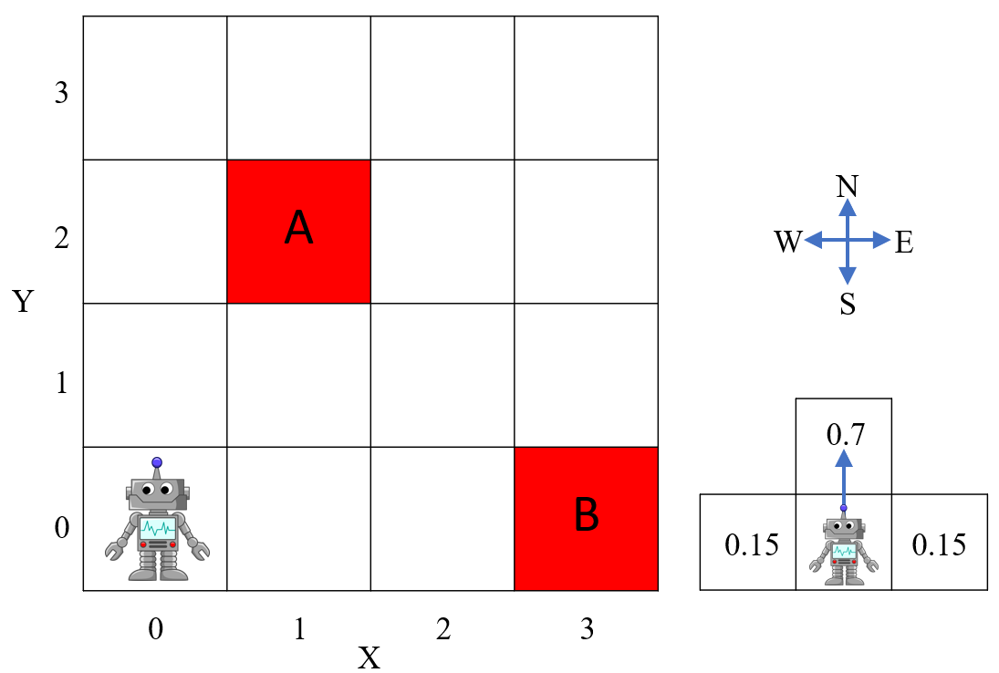
Figure 2: The $4\times 4$ grid world.

TABLE I: Initial state’s value versus error bounds $\epsilon_{1},\epsilon_{2}$ under different probability distributions $\mu_{1},\mu_{2}$ and $\bar{\mu}_{1},\bar{\mu}_{2}$.

	State size	518400	921600	1440000
Case 1: $\mu_{1},\mu_{2}$	$\epsilon_{1}$	0.343	0.2401	0.16807
	Value	0.43264	0.60645	0.60645
Case 2: $\bar{\mu}_{1},\bar{\mu}_{2}$	$\epsilon_{2}$	0.216	0.1296	0.07776
	Value	0.51411	0.62313	0.62313

Given different error bounds associated with corresponding of truncated vectors, we list the initial state’ values; that is, the probabilities of robot satisfying the given specification, in Table. I. The initial state’s value increases with decreasing error bounds $\epsilon_{1},\epsilon_{2}$ for both cases. However, the state space in the product MDP increases as the error bounds decrease too.

Given the error bound $\epsilon_{2}=0.07776$, we simulate trajectories in the case $2$ using the obtained policy. One trajectory is as follows:

$$(((0,0),\emptyset,\{b_{1},b_{2}\}),(\mathsf{Init},(0,0,0,0),\{b_{1},b_{2}\}))$$

$$\xrightarrow{\text{E}}((((0,0),\emptyset,\{b_{1},b_{2}\}),\text{E}),(\mathsf{Init},(0,0,0,0),\{b_{1},b_{2}\})))$$

$$\xrightarrow{b_{2}}((((1,0),\{b_{2}\},\{b_{1}\}),(\ell_{2},(1,0,1,0),\{b_{1}\}))$$

$$\xrightarrow{\text{E}}((((1,0),\{b_{2}\},\{b_{1}\}),\text{E}),(\ell_{2},(1,0,1,0),\{b_{1}\}))$$

$$\xrightarrow{b_{1}}(((1,1),\{b_{1}\},\emptyset),(\ell_{4},(0,0,0,1),\emptyset))$$

$$\xrightarrow{\text{N}}((((1,1),\{b_{1}\},\emptyset),\text{N}),(\ell_{4},(0,0,0,1),\emptyset))$$

$$\xrightarrow{\emptyset}(((1,2),\emptyset,\emptyset),(\ell_{3},(0,0,1,2),\emptyset))$$

The state is understood as, for example, $(((0,0),\emptyset,\{b_{1},b_{2}\})$ means that the robot is at position $(0,0)$, no external events happen in the most recent transition, and $b_{1},b_{2}$ have not been observed. Since in case 2 the atomic proposition $b_{2}$ has a higher probability of evaluating true every step until the first time $b_{2}$ is observed, the robot initially takes two consecutive actions E to go to the region $B$, and the bus 2 arrives after it took the first action E. However, due to the stochastic dynamics, the robot reaches state $(1,1)$ by taking action E at state $(1,0)$ while bus 1 arrives ($b_{1}$ evaluates true). Seeing it has more chance to reach bus 1, the robot takes action N to reach region $A$ instead of going to region $B$.

VI Conclusion

We investigated how to synthesize an optimal control policy for a new class of formal specifications which extend the Metric Interval Temporal Logic with a distribution eventuality operator . This new operator allows us to incorporate prior information of uncontrollable events in the interacting environments for decision-making with time-sensitive and event-triggered temporal constraints. We introduce a truncation of clocks to reduce the countably infinite MDP into a finite-state model and provide the error bound on the solution. In the future, we will investigate the scalability of our method. With abstraction methods such as region automaton [20], we can potentially reduce the size of the approximated finite-state model. We are also considering incorporating approximate dynamic programming [1] for large-scale MDPs to handle the issue of scalability.

References

• [1] L. Li and J. Fu, “Approximate dynamic programming with probabilistic temporal logic constraints,” in 2019 American Control Conference (ACC).   IEEE, 2019, pp. 1696–1703.
• [2] X. Ding, S. L. Smith, C. Belta, and D. Rus, “Optimal control of markov decision processes with linear temporal logic constraints,” IEEE Transactions on Automatic Control, vol. 59, no. 5, pp. 1244–1257, 2014.
• [3] E. A. Lee, “Cyber physical systems: Design challenges,” in 2008 11th IEEE international symposium on object and component-oriented real-time distributed computing (ISORC).   IEEE, 2008, pp. 363–369.
• [4] Z. Manna and A. Pnueli, Temporal Verification of Reactive Systems: Safety.   Berlin, Heidelberg: Springer-Verlag, 1995.
• [5] R. Koymans, “Specifying real-time properties with metric temporal logic,” Real-time systems, vol. 2, no. 4, pp. 255–299, 1990.
• [6] R. Alur, T. Feder, and T. A. Henzinger, “The benefits of relaxing punctuality,” Journal of the ACM (JACM), vol. 43, no. 1, pp. 116–146, 1996.
• [7] O. Maler and D. Nickovic, “Monitoring temporal properties of continuous signals,” in Formal Techniques, Modelling and Analysis of Timed and Fault-Tolerant Systems.   Springer, 2004, pp. 152–166.
• [8] A. Pnueli, “The temporal logic of programs,” in 18th Annual Symposium on Foundations of Computer Science (sfcs 1977).   IEEE, 1977, pp. 46–57.
• [9] L. Lindemann and D. V. Dimarogonas, “Robust motion planning employing signal temporal logic,” in 2017 American Control Conference (ACC).   IEEE, 2017, pp. 2950–2955.
• [10] G. Yang, C. Belta, and R. Tron, “Continuous-time signal temporal logic planning with control barrier functions,” in 2020 American Control Conference (ACC).   IEEE, 2020, pp. 4612–4618.
• [11] V. Raman, A. Donzé, D. Sadigh, R. M. Murray, and S. A. Seshia, “Reactive synthesis from signal temporal logic specifications,” in Proceedings of the 18th international conference on hybrid systems: Computation and control, 2015, pp. 239–248.
• [12] S. S. Farahani, V. Raman, and R. M. Murray, “Robust model predictive control for signal temporal logic synthesis,” IFAC-PapersOnLine, vol. 48, no. 27, pp. 323–328, 2015.
• [13] Z. Liu, J. Dai, B. Wu, and H. Lin, “Communication-aware motion planning for multi-agent systems from signal temporal logic specifications,” in 2017 American Control Conference (ACC).   IEEE, 2017, pp. 2516–2521.
• [14] A. Nikou, J. Tumova, and D. V. Dimarogonas, “Cooperative task planning of multi-agent systems under timed temporal specifications,” in American Control Conference.   IEEE, 2016, pp. 7104–7109.
• [15] P. Kapoor, A. Balakrishnan, and J. V. Deshmukh, “Model-based reinforcement learning from signal temporal logic specifications,” arXiv preprint arXiv:2011.04950, 2020.
• [16] S. Saha and A. A. Julius, “An milp approach for real-time optimal controller synthesis with metric temporal logic specifications,” in 2016 American Control Conference (ACC).   IEEE, 2016, pp. 1105–1110.
• [17] D. D’souza and P. Madhusudan, “Timed control synthesis for external specifications,” in Annual Symposium on Theoretical Aspects of Computer Science.   Springer, 2002, pp. 571–582.
• [18] Z. Xu, F. M. Zegers, B. Wu, W. Dixon, and U. Topcu, “Controller synthesis for multi-agent systems with intermittent communication. a metric temporal logic approach,” in 57th Annual Allerton Conference on Communication, Control, and Computing (Allerton).   IEEE, 2019, pp. 1015–1022.
• [19] A. Kovtunova and R. Peñaloza, “Cutting diamonds: A temporal logic with probabilistic distributions,” in Sixteenth International Conference on Principles of Knowledge Representation and Reasoning, 2018.
• [20] R. Alur and D. L. Dill, “A theory of timed automata,” Theoretical computer science, vol. 126, no. 2, pp. 183–235, 1994.
• [21] N. Bertrand, P. Bouyer, T. Brihaye, Q. Menet, C. Baier, M. Groesser, and M. Jurdzinski, “Stochastic Timed Automata,” Logical Methods in Computer Science, vol. 10, no. 4, p. 6, Dec. 2014.
• [22] O. Maler, D. Nickovic, and A. Pnueli, “From mitl to timed automata,” in International conference on formal modeling and analysis of timed systems.   Springer, 2006, pp. 274–289.
• [23] P. W. Holland and S. Leinhardt, “An exponential family of probability distributions for directed graphs,” Journal of the american Statistical association, vol. 76, no. 373, pp. 33–50, 1981.