Optimization of Graph Neural Networks:
Implicit Acceleration by Skip Connections and More Depth

Abstract

Graph Neural Networks (GNNs) have been studied through the lens of expressive power and generalization. However, their optimization properties are less well understood. We take the first step towards analyzing GNN training by studying the gradient dynamics of GNNs. First, we analyze linearized GNNs and prove that despite the non-convexity of training, convergence to a global minimum at a linear rate is guaranteed under mild assumptions that we validate on real-world graphs. Second, we study what may affect the GNNs’ training speed. Our results show that the training of GNNs is implicitly accelerated by skip connections, more depth, and/or a good label distribution. Empirical results confirm that our theoretical results for linearized GNNs align with the training behavior of nonlinear GNNs. Our results provide the first theoretical support for the success of GNNs with skip connections in terms of optimization, and suggest that deep GNNs with skip connections would be promising in practice.

1 Introduction

Graph Neural Networks (GNNs) (Gori et al., 2005; Scarselli et al., 2009) are an effective framework for learning with graphs. GNNs learn node representations on a graph by extracting high-level features not only from a node itself but also from a node’s surrounding subgraph. Specifically, the node representations are recursively aggregated and updated using neighbor representations  (Merkwirth & Lengauer, 2005; Duvenaud et al., 2015; Defferrard et al., 2016; Kearnes et al., 2016; Gilmer et al., 2017; Hamilton et al., 2017; Velickovic et al., 2018; Liao et al., 2020).

Recently, there has been a surge of interest in studying the theoretical aspects of GNNs to understand their success and limitations. Existing works have studied GNNs’ expressive power (Keriven & Peyré, 2019; Maron et al., 2019; Chen et al., 2019; Xu et al., 2019; Sato et al., 2019; Loukas, 2020), generalization capability (Scarselli et al., 2018; Du et al., 2019b; Xu et al., 2020; Garg et al., 2020), and extrapolation properties (Xu et al., 2021). However, the understanding of the optimization properties of GNNs has remained limited. For example, researchers working on the fundamental problem of designing more expressive GNNs hope and often empirically observe that more powerful GNNs better fit the training set (Xu et al., 2019; Sato et al., 2020; Vignac et al., 2020). Theoretically, given the non-convexity of GNN training, it is still an open question whether better representational power always translates into smaller training loss. This motivates the more general questions:

Can gradient descent find a global minimum for GNNs? What affects the speed of convergence in training?

In this work, we take an initial step towards answering the questions above by analyzing the trajectory of gradient descent, i.e., gradient dynamics or optimization dynamics. A complete understanding of the dynamics of GNNs, and deep learning in general, is challenging. Following prior works on gradient dynamics (Saxe et al., 2014; Arora et al., 2019a; Bartlett et al., 2019), we consider the linearized regime, i.e., GNNs with linear activation. Despite the linearity, key properties of nonlinear GNNs are present: The objective function is non-convex and the dynamics are nonlinear (Saxe et al., 2014; Kawaguchi, 2016). Moreover, we observe the learning curves of linear GNNs and ReLU GNNs are surprisingly similar, both converging to nearly zero training loss at the same linear rate (Figure 1). Similarly, prior works report comparable performance in node classification benchmarks even if we remove the non-linearities (Thekumparampil et al., 2018; Wu et al., 2019). Hence, understanding the dynamics of linearized GNNs is a valuable step towards understanding the general GNNs.

Our analysis leads to an affirmative answer to the first question. We establish that gradient descent training of a linearized GNN with squared loss converges to a global minimum at a linear rate. Experiments confirm that the assumptions of our theoretical results for global convergence hold on real-world datasets. The most significant contribution of our convergence analysis is on multiscale GNNs, i.e., GNN architectures that use skip connections to combine graph features at various scales (Xu et al., 2018; Li et al., 2019; Abu-El-Haija et al., 2020; Chen et al., 2020; Li et al., 2020). The skip connections introduce complex interactions among layers, and thus the resulting dynamics are more intricate. To our knowledge, our results are the first convergence results for GNNs with more than one hidden layer, with or without skip connections.

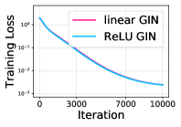
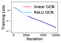
Figure 1: Training curves of linearized GNNs vs. ReLU GNNs on the Cora node classification dataset.

We then study what may affect the training speed of GNNs. First, for any fixed depth, GNNs with skip connections train faster. Second, increasing the depth further accelerates the training of GNNs. Third, faster training is obtained when the labels are more correlated with the graph features, i.e., labels contain “signal” instead of “noise”. Overall, experiments for nonlinear GNNs agree with the prediction of our theory for linearized GNNs.

Our results provide the first theoretical justification for the empirical success of multiscale GNNs in terms of optimization, and suggest that deeper GNNs with skip connections may be promising in practice. In the GNN literature, skip connections are initially motivated by the “over-smoothing” problem (Xu et al., 2018): via the recursive neighbor aggregation, node representations of a deep GNN on expander-like subgraphs would be mixing features from almost the entire graph, and may thereby “wash out” relevant local information. In this case, shallow GNNs may perform better. Multiscale GNNs with skip connections can combine and adapt to the graph features at various scales, i.e., the output of intermediate GNN layers, and such architectures are shown to help with this over-smoothing problem (Xu et al., 2018; Li et al., 2019, 2020; Abu-El-Haija et al., 2020; Chen et al., 2020). However, the properties of multiscale GNNs have mostly been understood at a conceptual level. Xu et al. (2018) relate the learned representations to random walk distributions and Oono & Suzuki (2020) take a boosting view, but they do not consider the optimization dynamics. We give an explanation from the lens of optimization. The training losses of deeper GNNs may be worse due to over-smoothing. In contrast, multiscale GNNs can express any shallower GNNs and fully exploit the power by converging to a global minimum. Hence, our results suggest that deeper GNNs with skip connections are guaranteed to train faster with smaller training losses.

We present our results on global convergence in Section 3, after introducing relevant background (Section 2). In Section 4, we compare the training speed of GNNs as a function of skip connections, depth, and the label distribution. All proofs are deferred to the Appendix.

2 Preliminaries

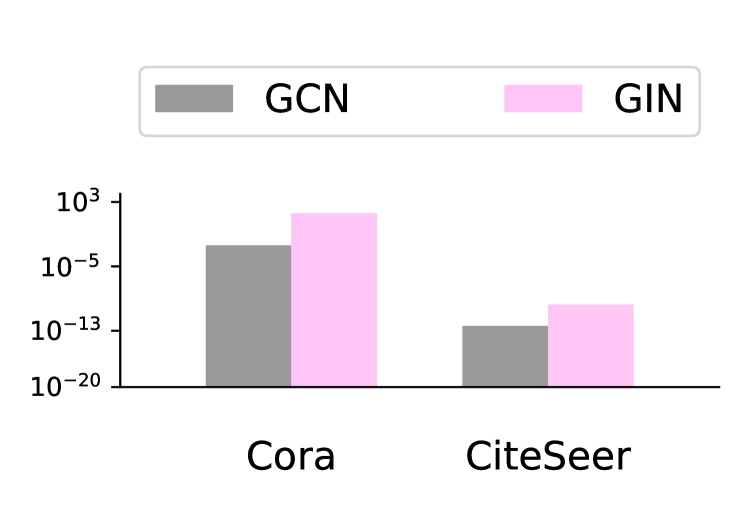
(a) Graph $\sigma^{2}_{\min}(X(S^{H})_{*\mathcal{I}})$

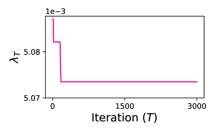
(b) Time-dependent $\lambda_{T}^{(H)}$

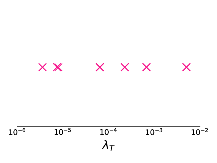
(c) $\lim_{T\rightarrow\infty}\lambda_{T}^{(H)}$ across training settings

Figure 2: Empirical validation of assumptions for global convergence of linear GNNs. Left panel confirms the graph condition $\sigma^{2}_{\min}(X(S^{H})_{*\mathcal{I}})>0$ for datasets Cora and Citeseer, and for models GCN and GIN. Middle panel shows the time-dependent $\lambda_{T}^{(H)}$ for one training setting (linear GCN on Cora). Each point in right panel is $\lambda_{T}^{(H)}>0$ at the last iteration for different training settings.

2.1 Notation and Background

We begin by introducing our notation. Let $G=\left(V,E\right)$ be a graph with $n$ vertices $V=\{v_{1},v_{2},\cdots,v_{n}\}$. Its adjacency matrix $A\in\mathbb{R}^{n\times n}$ has entries $A_{ij}=1$ if $(v_{i},v_{j})\in E$ and $0$ otherwise. The degree matrix associated with $A$ is $D=\mathop{\mathrm{diag}}\left(d_{1},d_{2},\dots,d_{n}\right)$ with $d_{i}=\sum_{j=1}^{n}A_{ij}$. For any matrix $M\in\mathbb{R}^{m\times m^{\prime}}$, we denote its $j$-th column vector by $M_{*j}\in\mathbb{R}^{m}$, its $i$-th row vector by $M_{i*}\in\mathbb{R}^{m^{\prime}}$, and its largest and smallest (i.e., $\min(m,m^{\prime})$-th largest) singular values by $\sigma_{\max}(M)$ and $\sigma_{\min}(M)$, respectively. The data matrix $X\in\mathbb{R}^{m_{x}\times n}$ has columns $X_{\ast j}$ corresponding to the feature vector of node $v_{j}$, with input dimension $m_{x}$.

The task of interest is node classification or regression. Each node $v_{i}\in V$ has an associated label $y_{i}\in\mathbb{R}^{m_{y}}$. In the transductive (semi-supervised) setting, we have access to training labels for only a subset $\mathcal{I}\subseteq[n]$ of nodes on $G$, and the goal is to predict the labels for the other nodes in $[n]\setminus\mathcal{I}$. Our problem formulation easily extends to the inductive setting by letting $\mathcal{I}=[n]$, and we can use the trained model for prediction on unseen graphs. Hence, we have access to $\bar{n}=|\mathcal{I}|\leq n$ training labels $Y=[y_{i}]_{i\in\mathcal{I}}\in\mathbb{R}^{m_{y}\times\bar{n}}$, and we train the GNN using $X,Y,G$. Additionally, for any $M\in\mathbb{R}^{m\times m^{\prime}}$, $\mathcal{I}$ may index sub-matrices $M_{*\mathcal{I}}=[M_{*i}]_{i\in\mathcal{I}}\in\mathbb{R}^{m\times\bar{n}}$ (when $m^{\prime}\geq n$) and $M_{\mathcal{I}*}=[M_{i*}]_{i\in\mathcal{I}}\in\mathbb{R}^{\bar{n}\times m}$ (when $m\geq n$).

Graph Neural Networks (GNNs) use the graph structure and node features to learn representations of nodes (Scarselli et al., 2009). GNNs maintain hidden representations $h^{v}_{(l)}\in\mathbb{R}^{m_{l}}$ for each node $v$, where $m_{l}$ is the hidden dimension on the $l$-th layer. We let $X_{(l)}=\big{[}h^{1}_{(l)},h^{2}_{(l)},\cdots,h^{n}_{(l)}\big{]}\in\mathbb{R}^{m_{l}\times n}$, and set $X_{(0)}$ as the input features $X$. The node hidden representations $X_{(l)}$ are updated by aggregating and transforming the neighbor representations:

$$X_{(l)}=\sigma\big{(}B_{(l)}X_{(l-1)}S\big{)}\in\mathbb{R}^{m_{l}\times n},$$ (1)

where $\sigma$ is a nonlinearity such as ReLU, $B_{(l)}\in\mathbb{R}^{m_{l}\times m_{l-1}}$ is the weight matrix, and $S\in\mathbb{R}^{n\times n}$ is the GNN aggregation matrix, whose formula depends on the exact variant of GNN. In Graph Isomorphism Networks (GIN) (Xu et al., 2019), $S=A+I_{n}$ is the adjacency matrix of $G$ with self-loop, where $I_{n}\in\mathbb{R}^{n\times n}$ is an identity matrix. In Graph Convolutional Networks (GCN) (Kipf & Welling, 2017), $S=\hat{D}^{-\frac{1}{2}}(A+I_{n})\hat{D}^{-\frac{1}{2}}$ is the normalized adjacency matrix, where $\hat{D}$ is the degree matrix of $A+I_{n}$.

2.2 Problem Setup

We first formally define linearized GNNs.

Definition 1.

(Linear GNN). Given data matrix $X\in\mathbb{R}^{m_{x}\times n}$, aggregation matrix $S\in\mathbb{R}^{n\times n}$, weight matrices $W\in\mathbb{R}^{m_{y}\times m_{H}}$, $B_{(l)}\in\mathbb{R}^{m_{l}\times m_{l-1}}$, and their collection $B=(B_{(1)},\dots,B_{(H)})$, a linear GNN with $H$ layers $f(X,W,B)\in\mathbb{R}^{m_{y}\times n}$ is defined as

$$f(X,W,B)=WX_{(H)},\quad X_{(l)}=B_{(l)}X_{(l-1)}S.$$ (2)

Throughout this paper, we refer multiscale GNNs to the commonly used Jumping Knowledge Network (JK-Net) (Xu et al., 2018), which connects the output of all intermediate GNN layers to the final layer with skip connections:

Definition 2.

(Multiscale linear GNN). Given data $X\in\mathbb{R}^{m_{x}\times n}$, aggregation matrix $S\in\mathbb{R}^{n\times n}$, weight matrices $W_{(l)}\in\mathbb{R}^{m_{y}\times m_{l}}$, $B_{(l)}\in\mathbb{R}^{m_{l}\times m_{l-1}}$ with $W=(W_{(0)},W_{(1)},\dots,W_{(H)})$, a multiscale linear GNN with $H$ layers $f(X,W,B)\in\mathbb{R}^{m_{y}\times n}$ is defined as

$$f(X,W,B) =\sum_{l=0}^{H}W_{(l)}X_{(l)},$$ (3)

$$X_{(l)} =B_{(l)}X_{(l-1)}S.$$ (4)

Given a GNN $f(\cdot)$ and a loss function $\ell(\cdot,Y)$, we can train the GNN by minimizing the training loss $L(W,B)$:

$$L(W,B)=\ell\big{(}f(X,W,B)_{*\mathcal{I}},Y\big{)},$$ (5)

where $f(X,W,B)_{*\mathcal{I}}$ corresponds to the GNN’s predictions on nodes that have training labels and thus incur training losses. The pair $(W,B)$ represents the trainable weights:

$$L(W,B)=L(W_{(1)},\dots,W_{(H)},B_{(1)},\dots,B_{(H)})$$

For completeness, we define the global minimum of GNNs.

Definition 3.

(Global minimum). For any $H\in\mathbb{N}_{0}$, $L^{*}_{H}$ is the global minimum value of the $H$-layer linear GNN $f$:

$$L^{*}_{H}=\inf_{W,B}\ell\big{(}f(X,W,B)_{*\mathcal{I}},Y\big{)}.$$ (6)

Similarly, we define $L^{*}_{1:H}$ as the global minimum value of the multiscale linear GNN $f$ with $H$ layers.

We are ready to present our main results on global convergence for linear GNNs and multiscale linear GNNs.

3 Convergence Analysis

In this section, we show that gradient descent training a linear GNN with squared loss, with or without skip connections, converges linearly to a global minimum. Our conditions for global convergence hold on real-world datasets and provably hold under assumptions, e.g., initialization.

In linearized GNNs, the loss $L(W,B)$ is non-convex (and non-invex) despite the linearity. The graph aggregation $S$ creates interaction among the data and poses additional challenges in the analysis. We show a fine-grained analysis of the GNN’s gradient dynamics can overcome these challenges. Following previous works on gradient dynamics (Saxe et al., 2014; Huang & Yau, 2020; Ji & Telgarsky, 2020; Kawaguchi, 2021), we analyze the GNN learning process via the gradient flow, i.e., gradient descent with infinitesimal steps: $\forall t\geq 0,$ the network weights evolve as

$$\frac{d}{dt}W_{t}=-\frac{\partial L}{\partial W}(W_{t},B_{t}),\quad\frac{d}{dt}B_{t}=-\frac{\partial L}{\partial B}(W_{t},B_{t}),$$ (7)

where $(W_{t},B_{t})$ represents the trainable parameters at time $t$ with initialization $(W_{0},B_{0})$.

3.1 Linearized GNNs

Theorem 1 states our result on global convergence for linearized GNNs without skip connections.

Theorem 1.

Let $f$ be an $H$-layer linear GNN and $\ell(q,Y)=\|q-Y\|^{2}_{F}$ where $q,Y\in\mathbb{R}^{m_{y}\times\bar{n}}$. Then, for any $T>0$,

$$L(W_{T},B_{T})-L^{*}_{H}$$ (8)

$$\leq(L(W_{0},B_{0})-L^{*}_{H})e^{-4\lambda_{T}^{(H)}\sigma^{2}_{\min}(X(S^{H})_{*\mathcal{I}})T},$$

where $\lambda_{T}^{(H)}$ is the smallest eigenvalue $\lambda_{T}^{(H)}:=\inf_{t\in[0,T]}\lambda_{\min}((\bar{B}^{(1:H)}_{t})^{\top}\bar{B}^{(1:H)}_{t})$ and $\bar{B}^{(1:l)}:=B_{(l)}B_{(l-1)}\cdots B_{(1)}$ for any $l\in\{0,\dots,H\}$ with $\bar{B}^{(1:0)}:=I$.

Proof.

(Sketch) We decompose the gradient dynamics into three components: the graph interaction, non-convex factors, and convex factors. We then bound the effects of the graph interaction and non-convex factors through $\sigma^{2}_{\min}(X(S^{H})_{*\mathcal{I}})$ and $\lambda_{\min}((\bar{B}^{(1:H)}_{t})^{\top}\bar{B}^{(1:H)}_{t})$ respectively. The complete proof is in Appendix A.1. ∎

Theorem 1 implies that convergence to a global minimum at a linear rate is guaranteed if $\sigma^{2}_{\min}(X(S^{H})_{*\mathcal{I}})>0$ and $\lambda_{T}>0$. The first condition on the product of $X$ and $S^{H}$ indexed by $\mathcal{I}$ only depends on the node features $X$ and the GNN aggregation matrix $S$. It is satisfied if $\mathop{\mathrm{rank}}(X(S^{H})_{*\mathcal{I}})=\min(m_{x},\bar{n})$, because $\sigma_{\min}(X(S^{H})_{*\mathcal{I}})$ is the $\min(m_{x},\bar{n})$-th largest singular value of $X(S^{H})_{*\mathcal{I}}\in\mathbb{R}^{m_{x}\times\bar{n}}$. The second condition $\lambda_{T}^{(H)}>0$ is time-dependent and requires a more careful treatment. Linear convergence is implied as long as $\lambda_{\min}((\bar{B}^{(1:H)}_{t})^{\top}\bar{B}^{(1:H)}_{t})\geq\epsilon>0$ for all times $t$ before stopping.

Empirical validation of conditions. We verify both the graph condition $\sigma^{2}_{\min}(X(S^{H})_{*\mathcal{I}})>0$ and the time-dependent condition $\lambda_{T}^{(H)}>0$ for (discretized) $T>0$. First, on the popular graph datasets, Cora and Citeseer (Sen et al., 2008), and the GNN models, GCN (Kipf & Welling, 2017) and GIN (Xu et al., 2019), we have $\sigma^{2}_{\min}(X(S^{H})_{*\mathcal{I}})>0$ (Figure 2(a)). Second, we train linear GCN and GIN on Cora and Citeseer to plot an example of how the $\lambda_{T}^{(H)}=\inf_{t\in[0,T]}\lambda_{\min}((\bar{B}^{(1:H)}_{t})^{\top}\bar{B}^{(1:H)}_{t})$ changes with respect to time $T$ (Figure 2(b)). We further confirm that $\lambda_{T}^{(H)}>0$ until convergence, $\lim_{T\rightarrow\infty}\lambda_{T}^{(H)}>0$ across different settings, e.g., datasets, depths, models (Figure 2(c)). Our experiments use the squared loss, random initialization, learning rate 1e-4, and set the hidden dimension to the input dimension (note that Theorem 1 assumes the hidden dimension is at least the input dimension). Further experimental details are in Appendix C. Along with Theorem 1, we conclude that linear GNNs converge linearly to a global minimum. Empirically, we indeed see both linear and ReLU GNNs converging at the same linear rate to nearly zero training loss in node classification tasks (Figure 1).

Guarantee via initialization. Besides the empirical verification, we theoretically show that a good initialization guarantees the time-dependent condition $\lambda_{T}>0$ for any $T>0$. Indeed, like other neural networks, GNNs do not converge to a global optimum with certain initializations: e.g., initializing all weights to zero leads to zero gradients and $\lambda_{T}^{(H)}=0$ for all $T$, and hence no learning. We introduce a notion of singular margin and say an initialization is good if it has a positive singular margin. Intuitively, a good initialization starts with an already small loss.

Definition 4.

(Singular margin). The initialization $(W_{0},B_{0})$ is said to have singular margin $\gamma>0$ with respect to a layer $l\in\{1,\dots,H\}$ if $\sigma_{\min}(B_{(l)}B_{(l-1)}\cdots B_{(1)})\geq\gamma$ for all $(W,B)$ such that $L(W,B)\leq L(W_{0},B_{0})$.

Proposition 1 then states that an initialization with positive singular margin $\gamma$ guarantees $\lambda_{T}^{(H)}\geq\gamma^{2}>0$ for all $T$:

Proposition 1.

Let $f$ be a linear GNN with $H$ layers and $\ell(q,Y)=\|q-Y\|^{2}_{F}$. If the initialization $(W_{0},B_{0})$ has singular margin $\gamma>0$ with respect to the layer $H$ and $m_{H}\geq m_{x}$, then $\lambda_{T}^{(H)}\geq\gamma^{2}$ for all $T\in[0,\infty)$.

Proposition 1 follows since $L(W_{t},B_{t})$ is non-increasing with respect to time $t$ (proof in Appendix A.2).

Relating to previous works, our singular margin is a generalized variant of the deficiency margin of linear feedforward networks (Arora et al., 2019a, Definition 2 and Theorem 1):

Proposition 2.

(Informal) If initialization $(W_{0},B_{0})$ has deficiency margin $c>0$, then it has singular margin $\gamma>0$.

The formal version of Proposition 2 is in Appendix A.3.

To summarize, Theorem 1 along with Proposition 1 implies that we have a prior guarantee of linear convergence to a global minimum for any graph with $\mathop{\mathrm{rank}}(X(S^{H})_{*\mathcal{I}})=\min(m_{x},\bar{n})$ and initialization $(W_{0},B_{0})$ with singular margin $\gamma>0$: i.e., for any desired $\epsilon>0$, we have that $L(W_{T},B_{T})-L^{*}_{H}\leq\epsilon$ for any $T$ such that

$$\quad\text{ }T\geq\frac{1}{4\gamma^{2}\sigma_{\min}^{2}(X(S^{H})_{*\mathcal{I}})}\log\frac{L(A_{0},B_{0})-L^{*}_{H}}{\epsilon}.$$ (9)

While the margin condition theoretically guarantees linear convergence, empirically, we have already seen that the convergence conditions of across different training settings for widely used random initialization.

Theorem 1 suggests that the convergence rate depends on a combination of data features $X$, the GNN architecture and graph structure via $S$ and $H$, the label distribution and initialization via $\lambda_{T}$. For example, GIN has better such constants than GCN on the Cora dataset with everything else held equal (Figure 2(a)). Indeed, in practice, GIN converges faster than GCN on Cora (Figure 1). In general, the computation and comparison of the rates given by Theorem 1 requires computation such as those in Figure 2. In Section 4, we will study an alternative way of comparing the speed of training by directly comparing the gradient dynamics.

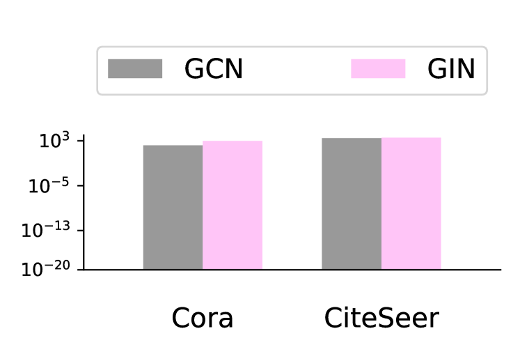
(a) Graph $\sigma^{2}_{\min}((G_{H})_{*\mathcal{I}})$

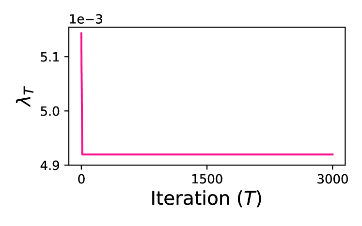
(b) Time-dependent $\lambda_{T}^{(1:H)}$

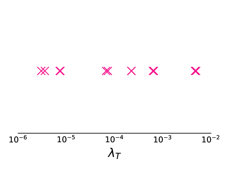
(c) $\lim_{T\rightarrow\infty}\lambda_{T}^{(1:H)}$ across training settings

Figure 3: Empirical validation of assumptions for global convergence of multiscale linear GNNs. Left panel confirms the graph condition $\sigma^{2}_{\min}((G_{H})_{*\mathcal{I}})>0$ for Cora and Citeseer, and for GCN and GIN. Middle panel shows the time-dependent $\lambda_{T}^{(1:H)}$ for one training setting (multiscale linear GCN on Cora). Each point in right panel is $\lambda_{T}^{(1:H)}>0$ at the last iteration for different training settings.

3.2 Multiscale Linear GNNs

Without skip connections, the GNNs under linearization still behave like linear feedforward networks with augmented graph features. With skip connections, the dynamics and analysis become much more intricate. The expressive power of multiscale linear GNNs changes significantly as depth increases. Moreover, the skip connections create complex interactions among different layers and graph structures of various scales in the optimization dynamics. Theorem 2 states our convergence results for multiscale linear GNNs in three cases: (i) a general form; (ii) a weaker condition for boundary cases that uses $\lambda_{T}^{H^{\prime}}$ instead of $\lambda_{T}^{1:H}$; (iii) a faster rate if we have monotonic expressive power as depth increases.

Theorem 2.

Let $f$ be a multiscale linear GNN with $H$ layers and $\ell(q,Y)=\|q-Y\|^{2}_{F}$ where $q,Y\in\mathbb{R}^{m_{y}\times\bar{n}}$. Let $\lambda_{T}^{(1:H)}:=\min_{0\leq l\leq H}\lambda_{T}^{(l)}$. For any $T>0$, the following hold:

1. (General). Let $G_{H}:=[X^{\top},(XS)^{\top},\dots,(XS^{H})^{\top}]^{\top}$ $\in\mathbb{R}^{(H+1)m_{x}\times n}$. Then

   $$L(W_{T},B_{T})-L^{*}_{1:H}$$ (10)

   $$\leq(L(W_{0},B_{0})-L^{*}_{1:H})e^{-4\lambda_{T}^{(1:H)}\sigma^{2}_{\min}((G_{H})_{*\mathcal{I}})T}.$$

2. (Boundary cases). For any $H^{\prime}\in\{0,1,\dots,H\}$,

   $$L(W_{T},B_{T})-L^{*}_{H^{\prime}}$$ (11)

   $$\leq(L(W_{0},B_{0})-L^{*}_{H^{\prime}})e^{-4\lambda_{T}^{(H^{\prime})}\sigma^{2}_{\min}(X(S^{H^{\prime}})_{*\mathcal{I}})T}.$$

3. (Monotonic expressive power). If there exist $l,l^{\prime}\in\{0,\dots,H\}$ with $l<l^{\prime}$ such that $L^{*}_{l}\geq L^{*}_{l+1}\geq\cdots\geq L^{*}_{l^{\prime}}$ or $L^{*}_{l}\leq L^{*}_{l+1}\leq\cdots\leq L^{*}_{l^{\prime}}$, then

   $$L(W_{T},B_{T})-L^{*}_{l^{\prime\prime}}$$ (12)

   $$\leq(L(W_{0},B_{0})-L^{*}_{l^{\prime\prime}})e^{-4\sum_{k=l}^{l^{\prime}}\lambda_{T}^{(k)}\sigma^{2}_{\min}(X(S^{k})_{*\mathcal{I}})T},$$

   where $l^{\prime\prime}=l$ if $L^{*}_{l}\geq L^{*}_{l+1}\geq\cdots\geq L^{*}_{l^{\prime}}$, and $l^{\prime\prime}=l^{\prime}$ if $L^{*}_{l}\leq L^{*}_{l+1}\leq\cdots\leq L^{*}_{l^{\prime}}$.

Proof.

(Sketch) A key observation in our proof is that the interactions of different scales cancel out to point towards a specific direction in the gradient dynamics induced in a space of the loss value. The complete proof is in Appendix A.4. ∎

Similar to Theorem 1 for linear GNNs, the most general form (i) of Theorem 2 implies that convergence to the global minimum value of the entire multiscale linear GNN $L_{1:H}^{*}$ at linear rate is guaranteed when $\sigma^{2}_{\min}((G_{H})_{*\mathcal{I}})>0$ and $\lambda_{T}^{(1:H)}>0$. The graph condition $\sigma^{2}_{\min}((G_{H})_{*\mathcal{I}})>0$ is satisfied if $\mathop{\mathrm{rank}}((G_{H})_{*\mathcal{I}})=\min(m_{x}(H+1),\bar{n})$. The time-dependent condition $\lambda_{T}^{(1:H)}>0$ is guaranteed if the initialization $(W_{0},B_{0})$ has singular margin $\gamma>0$ with respect to every layer (Proposition 3 is proved in Appendix A.5):

Proposition 3.

Let $f$ be a multiscale linear GNN and $\ell(q,Y)=\|q-Y\|^{2}_{F}$. If the initialization $(W_{0},B_{0})$ has singular margin $\gamma>0$ with respect to every layer $l\in[H]$ and $m_{l}\geq m_{x}$ for $l\in[H]$, then $\lambda_{T}^{(1:H)}\geq\gamma^{2}$ for all $T\in[0,\infty)$.

We demonstrate that the conditions of Theorem 2 (i) hold for real-world datasets, suggesting in practice multiscale linear GNNs converge linearly to a global minimum.

Empirical validation of conditions. On datasets Cora and Citeseer and for GNN models GCN and GIN, we confirm that $\sigma^{2}_{\min}((G_{H})_{*\mathcal{I}})>0$ (Figure 3(a)). Moreover, we train multiscale linear GCN and GIN on Cora and Citeseer to plot an example of how the $\lambda_{T}^{(1:H)}$ changes with respect to time $T$ (Figure 3(b)), and we confirm that at convergence, $\lambda_{T}^{(1:H)}>0$ across different settings (Figure 3(c)). Experimental details are in Appendix C.

Boundary cases. Because the global minimum value of multiscale linear GNNs $L_{1:H}^{*}$ can be smaller than that of linear GNNs $L_{H}^{*}$, the conditions in Theorem 2(i) may sometimes be stricter than those of Theorem 1. For example, in Theorem 2(i), we require $\lambda_{T}^{(1:H)}:=\min_{0\leq l\leq H}\lambda_{T}^{(l)}$ rather than $\lambda_{T}^{(H)}$ to be positive. If $\lambda_{T}^{(l)}=0$ for some $l$, then Theorem 2(i) will not guarantee convergence to $L_{1:H}^{*}$.

Although the boundary cases above did not occur on the tested real-world graphs (Figure 3), for theoretical interest, Theorem 2(ii) guarantees that in such cases, multiscale linear GNNs still converge to a value no worse than the global minimum value of non-multiscale linear GNNs. For any intermediate layer $H^{\prime}$, assuming $\sigma^{2}_{\min}(X(S^{H^{\prime}})_{*\mathcal{I}})>0$ and $\lambda_{T}^{(H^{\prime})}>0$, Theorem 2(ii) bounds the loss of the multiscale linear GNN $L(W_{T},B_{T})$ at convergence by the global minimum value $L^{*}_{H^{\prime}}$ of the corresponding linear GNN with $H^{\prime}$ layers.

Faster rate under monotonic expressive power. Theorem 2(iii) considers a special case that is likely in real graphs: the global minimum value of the non-multiscale linear GNN $L^{*}_{H^{\prime}}$ is monotonic as $H^{\prime}$ increases. Then (iii) gives a faster rate than (ii) and linear GNNs. For example, if the globally optimal value decreases as linear GNNs get deeper. i.e., $L^{*}_{0}\geq L^{*}_{1}\geq\cdots\geq L^{*}_{H}$, or vice versa, $L^{*}_{0}\leq L^{*}_{1}\leq\cdots\leq L^{*}_{H}$, then Theorem 2 (i) implies that

$$L(W_{T},B_{T})-L^{*}_{l}$$ (13)

$$\leq(L(W_{0},B_{0})-L^{*}_{l})e^{-4\sum_{k=0}^{H}\lambda_{T}^{(k)}\sigma^{2}_{\min}(X(S^{k})_{*\mathcal{I}})T},$$

where $l=0$ if $L^{*}_{0}\geq L^{*}_{1}\geq\cdots\geq L^{*}_{H}$, and $l=H$ if $L^{*}_{0}\leq L^{*}_{1}\leq\cdots\leq L^{*}_{H}$. Moreover, if the globally optimal value does not change with respect to the depth as $L^{*}_{1:H}=L^{*}_{1}=L^{*}_{2}=\cdots=L^{*}_{H}$, then we have

$$L(W_{T},B_{T})-L^{*}_{1:H}$$ (14)

$$\leq(L(W_{0},B_{0})-L^{*}_{1:H})e^{-4\sum_{k=0}^{H}\lambda_{T}^{(k)}\sigma^{2}_{\min}(X(S^{k})_{*\mathcal{I}})T}.$$

We obtain a faster rate for multiscale linear GNNs than for linear GNNs, as $e^{-4\sum_{k=0}^{H}\lambda_{T}^{(k)}\sigma^{2}_{\min}(X(S^{k})_{*\mathcal{I}})T}\leq e^{-4\lambda_{T}^{(H)}\sigma^{2}_{\min}(X(S^{H})_{*\mathcal{I}})T}$. Interestingly, unlike linear GNNs, multiscale linear GNNs in this case do not require any condition on initialization to obtain a prior guarantee on global convergence since $e^{-4\sum_{k=0}^{H}\lambda_{T}^{(k)}\sigma^{2}_{\min}(X(S^{k})_{*\mathcal{I}})T}\leq e^{-4\lambda_{T}^{(0)}\sigma^{2}_{\min}(X(S^{0})_{*\mathcal{I}})T}$ with $\lambda_{T}^{(0)}=1$ and $X(S^{0})_{*\mathcal{I}}=X_{*\mathcal{I}}$.

To summarize, we prove global convergence rates for multiscale linear GNNs (Thm. 2(i)) and experimentally validate the conditions. Part (ii) addresses boundary cases where the conditions of Part (i) do not hold. Part (iii) gives faster rates assuming monotonic expressive power with respect to depth. So far, we have shown multiscale linear GNNs converge faster than linear GNNs in the case of (iii). Next, we compare the training speed for more general cases.

4 Implicit Acceleration

(a) Multiscale vs. non-multiscale.

(b) Depth.

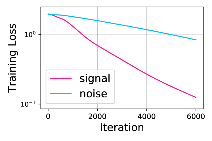
(c) Signal vs. noise.

Figure 4: Comparison of the training speed of GNNs. Left: Multiscale GNNs train faster than non-multiscale GNNs. Middle: Deeper GNNs train faster. Right: GNNs train faster when the labels have signals instead of random noise. The patterns above hold for both ReLU and linear GNNs. Additional results are in Appendix B.

In this section, we study how the skip connections, depth of GNN, and label distribution may affect the speed of training for GNNs. Similar to previous works (Arora et al., 2018), we compare the training speed by comparing the per step loss reduction $\frac{d}{dt}L(W_{t},B_{t})$ for arbitrary differentiable loss functions $\ell(\cdot,Y):\mathbb{R}^{m_{y}}\rightarrow\mathbb{R}$. Smaller $\frac{d}{dt}L(W_{t},B_{t})$ implies faster training. Loss reduction offers a complementary view to the convergence rates in Section 3, since it is instant and not an upper bound.

We present an analytical form of the loss reduction $\frac{d}{dt}L(W_{t},B_{t})$ for linear GNNs and multiscale linear GNNs. The comparison of training speed then follows from our formula for $\frac{d}{dt}L(W_{t},B_{t})$. For better exposition, we first introduce several notations. We let $\bar{B}^{(l^{\prime}:l)}=B_{(l)}B_{(l-1)}\cdots B_{(l^{\prime})}$ for all $l^{\prime}$ and $l$ where $\bar{B}^{(l^{\prime}:l)}=I$ if $l^{\prime}>l$. We also define

$$J_{(i,l),t}:=[\bar{B}^{(1:i-1)}_{t}\otimes(W_{(l),t}\bar{B}^{(i+1:l)}_{t})^{\top}],$$

$$F_{(l),t}:=[(\bar{B}^{(1:l)}_{t})^{\top}\bar{B}^{(1:l)}_{t}\otimes I_{m_{y}}]\succeq 0,$$

$$V_{t}:=\frac{\partial L(W_{t},B_{t})}{\partial\hat{Y}_{t}},$$

where $\hat{Y}_{t}:=f(X,W_{t},B_{t})_{*\mathcal{I}}$. For any vector $v\in\mathbb{R}^{m}$ and positive semidefinite matrix $M\in\mathbb{R}^{m\times m}$, we use $\|v\|_{M}^{2}:=v^{\top}Mv$. Intuitively, $V_{t}$ represents the derivative of the loss $L(W_{t},B_{t})$ with respect to the model output $\hat{Y}=f(X,W_{t},B_{t})_{*\mathcal{I}}$. $J_{(i,l),t}$ and $F_{(l),t}$ represent matrices that describe how the errors are propagated through the weights of the networks.

Theorem 3, proved in Appendix A.6, gives an analytical formula of loss reduction for linear GNNs and multiscale linear GNNs.

Theorem 3.

For any differentiable loss function $q\mapsto\ell(q,Y)$, the following hold for any $H\geq 0$ and $t\geq 0$:

1. (Non-multiscale) For $f$ as in Definition 1:

   $$\frac{d}{dt}L_{1}(W_{t},B_{t}) =-\scalebox{0.95}{$\displaystyle\left\|\operatorname{vec}\left[V_{t}(X(S^{H})_{*\mathcal{I}})^{\top}\right]\right\|_{F_{(H),t}}^{2}$}$$ (15)

2. (Multiscale) For $f$ as in Definition 2:

   $$\frac{d}{dt}L_{2}(W_{t},B_{t}) =\scalebox{0.95}{$\displaystyle-\sum_{l=0}^{H}\left\|\operatorname{vec}\left[V_{t}(X(S^{l})_{*\mathcal{I}})^{\top}\right]\right\|_{F_{(l),t}}^{2}$}$$ (16)

In what follows, we apply Theorem 3 to predict how different factors affect the training speed of GNNs.

4.1 Acceleration with Skip Connections

We first show that multiscale linear GNNs tend to achieve faster loss reduction $\frac{d}{dt}L_{2}(W_{t},B_{t})$ compared to the corresponding linear GNN without skip connections, $\frac{d}{dt}L_{1}(W_{t},B_{t})$. It follows from Theorem 3 that

$$\frac{d}{dt}L_{2}(W_{t},B_{t})-\frac{d}{dt}L_{1}(W_{t},B_{t})$$ (17)

$$\leq-\sum_{l=0}^{H-1}\left\|\operatorname{vec}\left[V_{t}(X(S^{l})_{*\mathcal{I}})^{\top}\right]\right\|_{F_{(l),t}}^{2},$$

if $\sum_{i=1}^{H}(\|a_{i}\|_{2}^{2}+2b_{i}^{\top}a_{i})\geq 0$, where $a_{i}=\sum_{l=i}^{H-1}J_{(i,l),t}\operatorname{vec}[V_{t}(X(S^{l})_{*\mathcal{I}})^{\top}]$, and $b_{i}=J_{(i,H),t}\operatorname{vec}[\allowbreak V_{t}(X(S^{H})_{*\mathcal{I}})^{\top}]$. The assumption of $\sum_{i=1}^{H}(\|a_{i}\|_{2}^{2}+\allowbreak 2b_{i}^{\top}a_{i})\allowbreak\geq\allowbreak 0$ is satisfied in various ways: for example, it is satisfied if the last layer’s term $b_{i}$ and the other layers’ terms $a_{i}$ are aligned as $b_{i}^{\top}a_{i}\geq 0$, or if the last layer’s term $b_{i}$ is dominated by the other layers’ terms $a_{i}$ as $2\|b_{i}\|_{2}\leq\|a_{i}\|_{2}$. Then equation (17) shows that the multiscale linear GNN decreases the loss value with strictly many more negative terms, suggesting faster training.

Empirically, we indeed observe that multiscale GNNs train faster (Figure 4(a)), both for (nonlinear) ReLU and linear GNNs. We verify this by training multiscale and non-multiscale, ReLU and linear GCNs on the Cora and Citeseer datasets with cross-entropy loss, learning rate 5e-5, and hidden dimension $32$. Results are in Appendix B.

4.2 Acceleration with More Depth

Our second finding is that deeper GNNs, with or without skip connections, train faster. For any differentiable loss function $q\mapsto\ell(q,Y)$, Theorem 3 states that the loss of the multiscale linear GNN decreases as

$$\frac{d}{dt}L(W_{t},B_{t}) =\scalebox{0.95}{$\displaystyle-\underbrace{\sum_{l=0}^{H}\underbrace{\left\|\operatorname{vec}\left[V_{t}(X(S^{l})_{*\mathcal{I}})^{\top}\right]\right\|_{F_{(l),t}}^{2}}_{\geq 0}}_{\begin{subarray}{c}\text{ further improvement as depth $H$ increases}\\ \end{subarray}}$}$$ (18)

In equation (18), we can see that the multiscale linear GNN achieves faster loss reduction as depth $H$ increases. A similar argument applies to non-multiscale linear GNNs.

Empirically too, deeper GNNs train faster (Figure 4(b)). Again, the acceleration applies to both (nonlinear) ReLU GNNs and linear GNNs. We verify this by training multiscale and non-multiscale, ReLU and linear GCNs with 2, 4, and 6 layers on the Cora and Citeseer datasets with learning rate 5e-5, hidden dimension $32$, and cross-entropy loss. Results are in Appendix B.

4.3 Label Distribution: Signal vs. Noise

Finally, we study how the labels affect the training speed. For the loss reduction (15) and (16), we argue that the norm of $V_{t}(X(S^{l})_{*\mathcal{I}})^{\top}$ tends to be larger for labels $Y$ that are more correlated with the graph features $X(S^{l})_{*\mathcal{I}}$, e.g., labels are signals instead of “noise”.

Without loss of generality, we assume $Y$ is normalized, e.g., one-hot labels. Here, $V_{t}=\frac{\partial L(A_{t},B_{t})}{\partial\hat{Y}_{t}}$ is the derivative of the loss with respect to the model output, e.g., $V_{t}=2(\hat{Y}_{t}-Y)$ for squared loss. If the rows of $Y$ are random noise vectors, then so are the rows of $V_{t}$, and they are expected to get more orthogonal to the columns of $(X(S^{l})_{*\mathcal{I}})^{\top}$ as $n$ increases. In contrast, if the labels $Y$ are highly correlated with the graph features $(X(S^{l})_{*\mathcal{I}})^{\top}$, i.e., the labels have signal, then the norm of $V_{t}(X(S^{l})_{*\mathcal{I}})^{\top}$ will be larger, implying faster training.

Our argument above focuses on the first term of the loss reduction, $\|V_{t}(X(S^{l})_{*\mathcal{I}})^{\top}\|_{\mathrm{F}}^{2}$. We empirically demonstrate that the scale of the second term, $\left\|\sum_{l=i}^{H}J_{(i,l),t}\operatorname{vec}\left[V_{t}(X(S^{l})_{*\mathcal{I}})^{\top}\right]\right\|_{2}^{2}$, is dominated by that of the first term (Figure 5). Thus, we can expect GNNs to train faster with signals than noise.

We train GNNs with the original labels of the dataset and random labels (i.e., selecting a class with uniform probability), respectively. The prediction of our theoretical analysis aligns with practice: training is much slower for random labels (Figure 4(c)). We verify this for mutliscale and non-multiscale, ReLU and linear GCNs on the Cora and Citseer datasets with learning rate 1e-4, hidden dimension $32$, and cross-entropy loss. Results are in Appendix B.

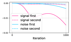
Figure 5: The scale of the first term dominates the second term of the loss reduction $\frac{d}{dt}L(W_{t},B_{t})$ for linear GNNs trained with the original labels vs. random labels on Cora.

5 Related Work

Theoretical analysis of linearized networks. The theoretical study of neural networks with some linearized components has recently drawn much attention. Tremendous efforts have been made to understand linear feedforward networks, in terms of their loss landscape (Kawaguchi, 2016; Hardt & Ma, 2017; Laurent & Brecht, 2018) and optimization dynamics (Saxe et al., 2014; Arora et al., 2019a; Bartlett et al., 2019; Du & Hu, 2019; Zou et al., 2020). Recent works prove global convergence rates for deep linear networks under certain conditions (Bartlett et al., 2019; Du & Hu, 2019; Arora et al., 2019a; Zou et al., 2020). For example, Arora et al. (2019a) assume the data to be whitened. Zou et al. (2020) fix the weights of certain layers during training. Our work is inspired by these works but differs in that our analysis applies to all learnable weights and does not require these specific assumptions, and we study the more complex GNN architecture with skip connections. GNNs consider the interaction of graph structures via the recursive message passing, but such structured, locally varying interaction is not present in feedforward networks. Furthermore, linear feedforward networks, even with skip connections, have the same expressive power as shallow linear models, a crucial condition in previous proofs (Bartlett et al., 2019; Du & Hu, 2019; Arora et al., 2019a; Zou et al., 2020). In contrast, the expressive power of multiscale linear GNNs can change significantly as depth increases. Accordingly, our proofs significantly differ from previous studies.

Another line of works studies the gradient dynamics of neural networks in the neural tangent kernel (NTK) regime (Jacot et al., 2018; Li & Liang, 2018; Allen-Zhu et al., 2019; Arora et al., 2019b; Chizat et al., 2019; Du et al., 2019a, c; Kawaguchi & Huang, 2019; Nitanda & Suzuki, 2021). With over-parameterization, the NTK remains almost constant during training. Hence, the corresponding neural network is implicitly linearized with respect to random features of the NTK at initialization (Lee et al., 2019; Yehudai & Shamir, 2019; Liu et al., 2020). On the other hand, our work needs to address nonlinear dynamics and changing expressive power.

Learning dynamics and optimization of GNNs. Closely related to our work, Du et al. (2019b); Xu et al. (2021) study the gradient dynamics of GNNs via the Graph NTK but focus on GNNs’ generalization and extrapolation properties. We instead analyze optimization. Only Zhang et al. (2020) also prove global convergence for GNNs, but for the one-hidden-layer case, and they assume a specialized tensor initialization and training algorithms. In contrast, our results work for any finite depth with no assumptions on specialized training. Other works aim to accelerate and stabilize the training of GNNs through normalization techniques (Cai et al., 2020) and importance sampling (Chen et al., 2018a, b; Huang et al., 2018; Chiang et al., 2019; Zou et al., 2019). Our work complements these practical works with a better theoretical understanding of GNN training.

6 Conclusion

This work studies the training properties of GNNs through the lens of optimization dynamics. For linearized GNNs with or without skip connections, despite the non-convex objective, we show that gradient descent training is guaranteed to converge to a global minimum at a linear rate. The conditions for global convergence are validated on real-world graphs. We further find out that skip connections, more depth, and/or a good label distribution implicitly accelerate the training of GNNs. Our results suggest deeper GNNs with skip connections may be promising in practice, and serve as a first foundational step for understanding the optimization of general GNNs.

Appendix A Proofs

In this section, we complete the proofs of our theoretical results. We show the proofs of Theorem 1 in Appendix A.1, Proposition 1 in Appendix A.2, Proposition 2 in Appendix A.3, Theorem 2 in Appendix A.4, Proposition 3 in Appendix A.5, and Theorem 3 in Appendix A.6.

Before starting our proofs, we first introduce additional notation used in the proofs. We define the corner cases on the products of $B$ as:

$$B_{(H)}B_{(H-1)}\cdots B_{(l+1)}:=I_{m_{l}}\quad\text{ if }H=l$$ (19)

$$B_{(H)}B_{(H-1)}\dots B_{(1)}:=I_{m_{x}}\quad\text{ if }H=0$$ (20)

$$B_{(l-1)}B_{(l-2)}\dots B_{(1)}:=I_{m_{x}}\quad\text{ if }l=1$$ (21)

Similarly, for any matrices $M_{(l)}$, we define $M_{(l)}M_{(l-1)}\cdots M_{(k)}:=I_{m}\text{ if }l<k,$ and $M_{(l)}M_{(l-1)}\cdots M_{(k)}:=M_{(k)}=M_{(l)}\text{ if }l=k.$ Given a scalar-valued variable $a\in\mathbb{R}$ and a matrix $M\in\mathbb{R}^{d\times d^{\prime}}$, we define

$$\frac{\partial a}{\partial M}=\begin{bmatrix}\frac{\partial a}{\partial M_{11}}&\cdots&\frac{\partial a}{\partial M_{1d^{\prime}}}\\ \vdots&\ddots&\vdots\\ \frac{\partial a}{\partial M_{d1}}&\cdots&\frac{\partial a}{\partial M_{dd^{\prime}}}\\ \end{bmatrix}\in\mathbb{R}^{d\times d^{\prime}},$$ (22)

where $M_{ij}$ represents the $(i,j)$-th entry of the matrix $M$. Given a vector-valued variable $a\in\mathbb{R}^{d}$ and a column vector $b\in\mathbb{R}^{d^{\prime}}$, we let

$$\frac{\partial a}{\partial b}=\begin{bmatrix}\frac{\partial a_{1}}{\partial b_{1}}&\cdots&\frac{\partial a_{1}}{\partial b_{d^{\prime}}}\\ \vdots&\ddots&\vdots\\ \frac{\partial a_{d}}{\partial b_{1}}&\cdots&\frac{\partial a_{d}}{\partial b_{d^{\prime}}}\\ \end{bmatrix}\in\mathbb{R}^{d\times d^{\prime}},$$ (23)

where $b_{i}$ represents the $i$-th entry of the column vector $b$. Similarly, given a vector-valued variable $a\in\mathbb{R}^{d}$ and a row vector $b\in\mathbb{R}^{1\times d^{\prime}}$, we write

$$\frac{\partial a}{\partial b}=\begin{bmatrix}\frac{\partial a_{1}}{\partial b_{11}}&\cdots&\frac{\partial a_{1}}{\partial b_{1d^{\prime}}}\\ \vdots&\ddots&\vdots\\ \frac{\partial a_{d}}{\partial b_{11}}&\cdots&\frac{\partial a_{d}}{\partial b_{1d^{\prime}}}\\ \end{bmatrix}\in\mathbb{R}^{d\times d^{\prime}},$$ (24)

where $b_{1i}$ represents the $i$-th entry of the row vector $b$. Finally, we recall the definition of the Kronecker product product of two matrices: for matrices $M\in\mathbb{R}^{d_{M}\times d_{M}^{\prime}}$ and $\bar{M}\in\mathbb{R}^{d_{\bar{M}}\times d^{\prime}_{\bar{M}}}$,

$$M\otimes\bar{M}=\begin{bmatrix}M_{11}\bar{M}&\cdots&M_{1d_{M}^{\prime}}\bar{M}\\ \vdots&\ddots\ &\vdots\\ M_{d_{M}1}\bar{M}&\cdots&M_{d_{M}d_{M}^{\prime}}\bar{M}\\ \end{bmatrix}\in\mathbb{R}^{d_{M}d_{\bar{M}}\times d_{M}^{\prime}d_{\bar{M}}^{\prime}}.$$ (25)

A.1 Proof of Theorem 1

We begin with a proof overview of Theorem 1. We first relate the gradients $\nabla_{W_{(H)}}L$ and $\nabla_{B_{(l)}}L$ to the gradient $\nabla_{(H)}L$, which is defined by

$$\nabla_{(H)}L(W,B):=\frac{\partial L(W,B)}{\partial\hat{Y}}(X(S^{H})_{*\mathcal{I}})^{\top}\in\mathbb{R}^{m_{y}\times m_{x}}.$$

Using the proven relation of $(\nabla_{W_{(H)}}L,\nabla_{B_{(l)}}L)$ and $\nabla_{(H)}L$, we first analyze the dynamics induced in the space of $W_{(l)}B_{(l)}B_{(l-1)}\cdots B_{(1)}$ in Appendix A.1.1, and then the dynamics induced int the space of loss value $L(W,B)$ in Appendix A.1.2. Finally, we complete the proof by using the assumption of employing the square loss in Appendix A.1.3.

Let $W_{(H)}=W$ (during the proof of Theorem 1). We first prove the relationship of the gradients $\nabla_{W_{(H)}}L$, $\nabla_{B_{(l)}}L$ and $\nabla_{(H)}L$ in the following lemma:

Lemma 1.

Let $f$ be an $H$-layer linear GNN and $\ell(q,Y)=\|q-Y\|^{2}_{F}$ where $q,Y\in\mathbb{R}^{m_{y}\times\bar{n}}$. Then, for any $(W,B)$,

$$\nabla_{W_{(H)}}L(W,B) =\nabla_{(H)}L(W,B)(B_{(H)}B_{(H-1)}\dots B_{(1)})^{\top}\in\mathbb{R}^{m_{y}\times m_{l}},$$ (26)

and

$$\nabla_{B_{(l)}}L(W,B) =(W_{(H)}B_{(H)}B_{(H-1)}\cdots B_{(l+1)})^{\top}\nabla_{(H)}L(W,B)(B_{(l-1)}B_{(l-2)}\dots B_{(1)})^{\top}\in\mathbb{R}^{m_{l}\times m_{l-1}},$$ (27)

Proof of Lemma 1.

From Definition 1, we have $\hat{Y}=f(X,W,B)_{*\mathcal{I}}=W_{(H)}(X_{(H)})_{*\mathcal{I}}$ where $X_{(l)}=B_{(l)}X_{(l-1)}S$. Using this definition, we can derive the formula of $\frac{\partial\operatorname{vec}[\hat{Y}]}{\partial\operatorname{vec}[W_{(H)}]}\in\mathbb{R}^{m_{y}n\times m_{y}m_{\bar{H}}}$ as:

$$\frac{\partial\operatorname{vec}[\hat{Y}]}{\partial\operatorname{vec}[W_{(H)}]} =\frac{\partial}{\partial\operatorname{vec}[W_{(H)}]}\operatorname{vec}[W_{(H)}(X_{(H)})_{*\mathcal{I}}]$$

$$=\frac{\partial}{\partial\operatorname{vec}[W_{(H)}]}[((X_{(H)})_{*\mathcal{I}})^{\top}\otimes I_{m_{y}}]\operatorname{vec}[W_{(H)}]=[((X_{(H)})_{*\mathcal{I}})^{\top}\otimes I_{m_{y}}]\in\mathbb{R}^{m_{y}n\times m_{y}m_{\bar{H}}}$$ (28)

We will now derive the formula of $\frac{\partial\operatorname{vec}[\hat{Y}]}{\partial\operatorname{vec}[B_{(l)}]}\in\mathbb{R}^{m_{y}n\times m_{l}m_{l-1}}$:

$$\frac{\partial\operatorname{vec}[\hat{Y}]}{\partial\operatorname{vec}[B_{(l)}]} =\frac{\partial}{\partial\operatorname{vec}[B_{(l)}]}\operatorname{vec}[W_{(H)}(X_{(H)})_{*\mathcal{I}}]$$

$$=\frac{\partial}{\partial\operatorname{vec}[B_{(l)}]}[I_{n}\otimes W_{(H)}]\operatorname{vec}[(X_{(H)})_{*\mathcal{I}}]$$

$$=[I_{n}\otimes W_{(H)}]\frac{\partial\operatorname{vec}[(X_{(H)})_{*\mathcal{I}}]}{\partial\operatorname{vec}[B_{(l)}]}$$

$$=[I_{n}\otimes W_{(H)}]\frac{\partial\operatorname{vec}[(X_{(H)})_{*\mathcal{I}}]}{\partial\operatorname{vec}[X_{(l)}]}\frac{\partial\operatorname{vec}[X_{(l)}]}{\partial\operatorname{vec}[B_{(l)}]}$$

$$=[I_{n}\otimes W_{(H)}]\frac{\partial\operatorname{vec}[(X_{(H)})_{*\mathcal{I}}]}{\partial\operatorname{vec}[X_{(l)}]}\frac{\partial\operatorname{vec}[B_{(l)}X_{(l-1)}S]}{\partial\operatorname{vec}[B_{(l)}]}$$

$$=[I_{n}\otimes W_{(H)}]\frac{\partial\operatorname{vec}[(X_{(H)})_{*\mathcal{I}}]}{\partial\operatorname{vec}[X_{(l)}]}\frac{\partial[(X_{(l-1)}S)^{\top}\otimes I_{m_{l}}]\operatorname{vec}[B_{(l)}]}{\partial\operatorname{vec}[B_{(l)}]}$$

$$=[I_{n}\otimes W_{(H)}]\frac{\partial\operatorname{vec}[(X_{(H)})_{*\mathcal{I}}]}{\partial\operatorname{vec}[X_{(l)}]}[(X_{(l-1)}S)^{\top}\otimes I_{m_{l}}]$$ (29)

Here, we have that

$$\operatorname{vec}[(X_{(H)})_{*\mathcal{I}}]=\operatorname{vec}[B_{(H)}X_{(H-1)}S_{*\mathcal{I}}]=\operatorname{vec}[(S^{\top})_{\mathcal{I}*}\otimes B_{(H)}]\operatorname{vec}[X_{(H-1)}].$$ (30)

and

$$\operatorname{vec}[X_{(H)}]=\operatorname{vec}[B_{(H)}X_{(H-1)}S_{*\mathcal{I}}]=\operatorname{vec}[S\otimes B_{(H)}]\operatorname{vec}[X_{(H-1)}].$$ (31)

By recursively applying (31), we have that

$$\operatorname{vec}[(X_{(H)})_{*\mathcal{I}}] =\operatorname{vec}[(S^{\top})_{\mathcal{I}*}\otimes B_{(H)}]\operatorname{vec}[S^{\top}\otimes B_{(H-1)}]\cdots\operatorname{vec}[S^{\top}\otimes B_{(l+1)}]\operatorname{vec}[X_{(l)}]$$

$$=\operatorname{vec}[((S^{H-l})^{\top})_{\mathcal{I}*}\otimes B_{(H)}B_{(H-1)}\cdots B_{(l+1)}]\operatorname{vec}[X_{(l)}],$$

where

$$B_{(H)}B_{(H-1)}\cdots B_{(l+1)}:=I_{m_{l}}\quad\text{ if $H=l$.}$$

Therefore,

$$\frac{\partial\operatorname{vec}[(X_{(H)})_{*\mathcal{I}}]}{\partial\operatorname{vec}[X_{(l)}]} =\operatorname{vec}[((S^{H-l})^{\top})_{\mathcal{I}*}\otimes B_{(H)}B_{(H-1)}\cdots B_{(l+1)}].$$ (32)

Combining (A.1) and (32) yields

$$\frac{\partial\operatorname{vec}[\hat{Y}]}{\partial\operatorname{vec}[B_{(l)}]} =[I_{n}\otimes W_{(H)}]\frac{\partial\operatorname{vec}[(X_{(H)})_{*\mathcal{I}}]}{\partial\operatorname{vec}[X_{(l)}]}[(X_{(l-1)}S)^{\top}\otimes I_{m_{l}}]$$

$$=[I_{n}\otimes W_{(H)}]\operatorname{vec}[((S^{H-l})^{\top})_{\mathcal{I}*}\otimes B_{(H)}B_{(H-1)}\cdots B_{(l+1)}][(X_{(l-1)}S)^{\top}\otimes I_{m_{l}}]$$

$$=[(X_{(l-1)}(S^{H-l+1})_{*\mathcal{I}})^{\top}\otimes W_{(H)}B_{(H)}B_{(H-1)}\cdots B_{(l+1)}]\in\mathbb{R}^{m_{y}n\times m_{l}m_{l-1}}.$$ (33)

Using (A.1), we will now derive the formula of $\nabla_{W_{(H)}}L(W,B)\in\mathbb{R}^{m_{y}\times m_{H}}$:

$$\frac{\partial L(W,B)}{\partial\operatorname{vec}[W_{(H)}]}=\frac{\partial L(W,B)}{\partial\operatorname{vec}[\hat{Y}]}\frac{\partial\operatorname{vec}[\hat{Y}]}{\partial\operatorname{vec}[W_{(H)}]}=\frac{\partial L(W,B)}{\partial\operatorname{vec}[\hat{Y}]}[(X_{(H)})_{*\mathcal{I}}^{\top}\otimes I_{m_{y}}]$$

Thus, with $\frac{\partial L(W,B)}{\partial\hat{Y}}\in\mathbb{R}^{m_{y}\times n}$,

$$\nabla_{\operatorname{vec}[W_{(H)}]}L(W,B) =\left(\frac{\partial L(W,B)}{\partial\operatorname{vec}[W_{(H)}]}\right)^{\top}$$

$$=[(X_{(H)})_{*\mathcal{I}}\otimes I_{m_{y}}]\left(\frac{\partial L(W,B)}{\partial\operatorname{vec}[\hat{Y}]}\right)^{\top}$$

$$=[(X_{(H)})_{*\mathcal{I}}\otimes I_{m_{y}}]\operatorname{vec}\left[\frac{\partial L(W,B)}{\partial\hat{Y}}\right]$$

$$=\operatorname{vec}\left[\frac{\partial L(W,B)}{\partial\hat{Y}}(X_{(H)})_{*\mathcal{I}}^{\top}\right]\in\mathbb{R}^{m_{y}m_{H}}.$$

Therefore,

$$\nabla_{W_{(H)}}L(W,B) =\frac{\partial L(W,B)}{\partial\hat{Y}}(X_{(H)})_{*\mathcal{I}}^{\top}\in\mathbb{R}^{m_{y}\times m_{H}}.$$ (34)

Using (A.1), we will now derive the formula of $\nabla_{B_{(l)}}L(W,B)\in\mathbb{R}^{m_{l}\times m_{l-1}}$:

$$\frac{\partial L(W,B)}{\partial\operatorname{vec}[B_{(l)}]}=\frac{\partial L(W,B)}{\partial\operatorname{vec}[\hat{Y}]}\frac{\partial\operatorname{vec}[\hat{Y}]}{\partial\operatorname{vec}[B_{(l)}]}=\frac{\partial L(W,B)}{\partial\operatorname{vec}[\hat{Y}]}[(X_{(l-1)}(S^{H-l+1})_{*\mathcal{I}})^{\top}\otimes W_{(H)}B_{(H)}B_{(H-1)}\cdots B_{(l+1)}].$$

Thus, with $\frac{\partial L(W,B)}{\partial\hat{Y}}\in\mathbb{R}^{m_{y}\times n}$,

$$\nabla_{\operatorname{vec}[B_{(l)}]}L(W,B) =\left(\frac{\partial L(W,B)}{\partial\operatorname{vec}[B_{(l)}]}\right)^{\top}$$

$$=[X_{(l-1)}(S^{H-l+1})_{*\mathcal{I}}\otimes(W_{(H)}B_{(H)}B_{(H-1)}\cdots B_{(l+1)})^{\top}]\left(\frac{\partial L(W,B)}{\partial\operatorname{vec}[\hat{Y}]}\right)^{\top}$$

$$=[X_{(l-1)}(S^{H-l+1})_{*\mathcal{I}}\otimes(W_{(H)}B_{(H)}B_{(H-1)}\cdots B_{(l+1)})^{\top}]\operatorname{vec}\left[\frac{\partial L(W,B)}{\partial\hat{Y}}\right]$$

$$=\operatorname{vec}\left[(W_{(H)}B_{(H)}B_{(H-1)}\cdots B_{(l+1)})^{\top}\frac{\partial L(W,B)}{\partial\hat{Y}}(X_{(l-1)}(S^{H-l+1})_{*\mathcal{I}})^{\top}\right]\in\mathbb{R}^{m_{l}m_{l-1}}.$$

Therefore,

$$\nabla_{B_{(l)}}L(W,B)=(W_{(H)}B_{(H)}B_{(H-1)}\cdots B_{(l+1)})^{\top}\frac{\partial L(W,B)}{\partial\hat{Y}}(X_{(l-1)}(S^{H-l+1})_{*\mathcal{I}})^{\top}\in\mathbb{R}^{m_{l}\times m_{l-1}}.$$ (35)

With (34) and (35), we are now ready to prove the statement of this lemma by introducing the following notation:

$$\nabla_{(l)}L(W,B):=\frac{\partial L(W,B)}{\partial\hat{Y}}(X(S^{l})_{*\mathcal{I}})^{\top}\in\mathbb{R}^{m_{y}\times m_{x}}.$$

Using this notation along with (34)

$$\nabla_{W_{(H)}}L(W,B) =\frac{\partial L(W,B)}{\partial\hat{Y}}(X_{(H)})_{*\mathcal{I}}^{\top}$$

$$=\frac{\partial L(W,B)}{\partial\hat{Y}}(B_{(H)}X_{(H-1)}(S)_{*\mathcal{I}})^{\top}$$

$$=\frac{\partial L(W,B)}{\partial\hat{Y}}(B_{(H)}B_{(H-1)}\dots B_{(1)}X(S^{H})_{*\mathcal{I}})^{\top}$$

$$=\nabla_{(H)}L(W,B)(B_{(H)}B_{(H-1)}\dots B_{(1)})^{\top},$$

Similarly, using (35),

$$\nabla_{B_{(l)}}L(W,B) =(W_{(H)}B_{(H)}B_{(H-1)}\cdots B_{(l+1)})^{\top}\frac{\partial L(W,B)}{\partial\hat{Y}}(X_{(l-1)}(S^{H-l+1})_{*\mathcal{I}})^{\top}$$

$$=(W_{(H)}B_{(H)}B_{(H-1)}\cdots B_{(l+1)})^{\top}\frac{\partial L(W,B)}{\partial\hat{Y}}(B_{(l-1)}B_{(l-2)}\dots B_{(1)}X(S^{l-1}S^{H-l+1})_{*\mathcal{I}})^{\top}$$

$$=(W_{(H)}B_{(H)}B_{(H-1)}\cdots B_{(l+1)})^{\top}\frac{\partial L(W,B)}{\partial\hat{Y}}(B_{(l-1)}B_{(l-2)}\dots B_{(1)}X(S^{H})_{*\mathcal{I}})^{\top}$$

$$=(W_{(H)}B_{(H)}B_{(H-1)}\cdots B_{(l+1)})^{\top}\nabla_{(H)}L(W,B)(B_{(l-1)}B_{(l-2)}\dots B_{(1)})^{\top}$$

where $B_{(l-1)}B_{(l-2)}\dots B_{(1)}:=I_{m_{x}}$ if $l=1$.

∎

By using Lemma 1, we complete the proof of Theorem 1 in the following.

A.1.1 Dynamics induced in the space of $W_{(l)}B_{(l)}B_{(l-1)}\cdots B_{(1)}$

We now consider the dynamics induced in the space of $W_{(l)}B_{(l)}B_{(l-1)}\cdots B_{(1)}$. We first consider the following discrete version of the dynamics:

$$W_{(H)}^{\prime}=W_{(H)}-\alpha\nabla_{W_{(H)}}L(W,B)$$

$$B_{(l)}^{\prime}=B_{(l)}-\alpha\nabla_{B_{(l)}}L(W,B).$$

This dynamics induces the following dynamics:

$$W_{(H)}^{\prime}B_{(H)}^{\prime}B_{(H-1)}^{\prime}\cdots B_{(1)}^{\prime}=(W_{(H)}-\alpha\nabla_{W_{(H)}}L(W,B))(B_{(H)}-\alpha\nabla_{B_{(H)}}L(W,B))\cdots(B_{(1)}-\alpha\nabla_{B_{(1)}}L(W,B)).$$

Define

$$Z_{(H)}:=W_{(H)}B_{(H)}B_{(H-1)}\cdots B_{(1)},$$

and

$$Z_{(H)}^{\prime}:=W_{(H)}^{\prime}B_{(H)}^{\prime}B_{(H-1)}^{\prime}\cdots B_{(1)}^{\prime}.$$

Then, we can rewrite

$$Z_{(H)}^{\prime}=(W_{(H)}-\alpha\nabla_{W_{(H)}}L(W,B))(B_{(H)}-\alpha\nabla_{B_{(H)}}L(W,B))\cdots(B_{(1)}-\alpha\nabla_{B_{(1)}}L(W,B)).$$

By expanding the multiplications, this can be written as:

$$Z_{(H)}^{\prime}=Z_{(H)}-\alpha\nabla_{W_{(H)}}L(W,B)B_{(H)}\cdots B_{(1)}-\alpha\sum_{i=1}^{H}W_{(H)}B_{(H)}\cdots B_{(i+1)}\nabla_{B_{(i)}}L(W,B)B_{(i-1)}\cdots B_{(1)}+O(\alpha^{2}).$$

By vectorizing both sides,

$$\operatorname{vec}[Z_{(H)}^{\prime}]-\operatorname{vec}[Z_{(H)}]$$

$$=-\alpha\operatorname{vec}[\nabla_{W_{(H)}}L(W,B)B_{(H)}\cdots B_{(1)}]-\alpha\sum_{i=1}^{H}\operatorname{vec}[W_{(H)}B_{(H)}\cdots B_{(i+1)}\nabla_{B_{(i)}}L(W,B)B_{(i-1)}\cdots B_{(1)}]+O(\alpha^{2}).$$

Here, using the formula of $\nabla_{W_{(H)}}L(W,B)$ and $\nabla_{B_{(H)}}L(W,B)$, we have that

$$\operatorname{vec}[\nabla_{W_{(H)}}L(W,B)B_{(H)}\cdots B_{(1)}] =\operatorname{vec}[\nabla_{(H)}L(W,B)(B_{(H)}\dots B_{(1)})^{\top}B_{(H)}\cdots B_{(1)}]$$

$$=[(B_{(H)}\dots B_{(1)})^{\top}B_{(H)}\cdots B_{(1)}\otimes I_{m_{y}}]\operatorname{vec}[\nabla_{(H)}L(W,B)],$$

and

$$\sum_{i=1}^{H}\operatorname{vec}[W_{(H)}B_{(H)}\cdots B_{(i+1)}\nabla_{B_{(i)}}L(W,B)B_{(i-1)}\cdots B_{(1)}]$$

$$=\sum_{i=1}^{H}\operatorname{vec}\left[W_{(H)}B_{(H)}\cdots B_{(i+1)}(W_{(H)}B_{(H)}\cdots B_{(i+1)})^{\top}\nabla_{(H)}L(W,B)(B_{(i-1)}\dots B_{(1)})^{\top}B_{(i-1)}\cdots B_{(1)}\right]$$

$$=\sum_{i=1}^{H}[(B_{(i-1)}\dots B_{(1)})^{\top}B_{(i-1)}\cdots B_{(1)}\otimes W_{(H)}B_{(H)}\cdots B_{(i+1)}(W_{(H)}B_{(H)}\cdots B_{(i+1)})^{\top}]\operatorname{vec}\left[\nabla_{(H)}L(W,B)\right].$$

Summarizing above,

$$\operatorname{vec}[Z_{(H)}^{\prime}]-\operatorname{vec}[Z_{(H)}]$$

$$=-\alpha[(B_{(H)}\dots B_{(1)})^{\top}B_{(H)}\cdots B_{(1)}\otimes I_{m_{y}}]\operatorname{vec}[\nabla_{(H)}L(W,B)]$$

$$\hskip 12.0pt-\alpha\sum_{i=1}^{H}[(B_{(i-1)}\dots B_{(1)})^{\top}B_{(i-1)}\cdots B_{(1)}\otimes W_{(H)}B_{(H)}\cdots B_{(i+1)}(W_{(H)}B_{(H)}\cdots B_{(i+1)})^{\top}]\operatorname{vec}\left[\nabla_{(H)}L(W,B)\right]$$

$$\hskip 12.0pt+O(\alpha^{2})$$

Therefore, the induced continuous dynamics of $Z_{(H)}=W_{(H)}B_{(H)}B_{(H-1)}\cdots B_{(1)}$ is

$$\frac{d}{dt}\operatorname{vec}[Z_{(H)}]=-F_{(H)}\operatorname{vec}[\nabla_{(H)}L(W,B)]-\left(\sum_{i=1}^{H}J_{(i,H)}^{\top}J_{(i,H)}\right)\operatorname{vec}\left[\nabla_{(H)}L(W,B)\right],$$

where

$$F_{(H)}=[(B_{(H)}\dots B_{(1)})^{\top}B_{(H)}\cdots B_{(1)}\otimes I_{m_{y}}],$$

and

$$J_{(i,H)}=[B_{(i-1)}\dots B_{(1)}\otimes(W_{(H)}B_{(H)}\cdots B_{(i+1)})^{\top}].$$

This is because

$$J_{(i,H)}^{\top}J_{(i,H)} =[(B_{(i-1)}\dots B_{(1)})^{\top}\otimes W_{(H)}B_{(H)}\cdots B_{(i+1)}][B_{(i-1)}\dots B_{(1)}\otimes(W_{(H)}B_{(H)}\cdots B_{(i+1)})^{\top}]$$

$$=[(B_{(i-1)}\dots B_{(1)})^{\top}B_{(i-1)}\dots B_{(1)}\otimes W_{(H)}B_{(H)}\cdots B_{(i+1)}(W_{(H)}B_{(H)}\cdots B_{(i+1)})^{\top}].$$

A.1.2 Dynamics induced int the space of loss value $L(W,B)$

We now analyze the dynamics induced int the space of loss value $L(W,B)$. Using chain rule,

$$\frac{d}{dt}L(W,B) =\frac{d}{dt}L_{0}(Z_{(H)})$$

$$=\frac{\partial L_{0}(Z_{(H)})}{\partial\operatorname{vec}[Z_{(H)}]}\frac{d\operatorname{vec}[Z_{(H)}]}{dt},$$

where

$$L_{0}(Z_{(H)})=\ell(f_{0}(X,Z_{(H)})_{*\mathcal{I}},Y),\ \ f_{0}(X,Z_{(H)})=Z_{(H)}XS^{H},\ \text{ and }Z_{(H)}=W_{(H)}B_{(H)}B_{(H-1)}\cdots B_{(1)}.$$

Since $f_{0}(X,Z_{(H)})=f(X,W,B)=\hat{Y}$ and $L_{0}(Z_{(H)})=L(W,B)$, we have that

$$\left(\frac{\partial L_{0}(Z_{(H)})}{\partial\operatorname{vec}[Z_{(H)}]}\right)^{\top} =\left(\frac{\partial L(W,B)}{\partial\operatorname{vec}[\hat{Y}]}\frac{\partial\operatorname{vec}[\hat{Y}]}{\partial\operatorname{vec}[Z_{(H)}]}\right)^{\top}$$

$$=\left(\frac{\partial L(W,B)}{\partial\operatorname{vec}[\hat{Y}]}\left(\frac{\partial}{\partial\operatorname{vec}[Z_{(H)}]}[(X(S^{H})_{*\mathcal{I}})^{\top}\otimes I_{m_{y}}]\operatorname{vec}[Z_{(H)}]\right)\right)^{\top}$$

$$=[X(S^{H})_{*\mathcal{I}}\otimes I_{m_{y}}]\operatorname{vec}\left[\frac{\partial L(W,B)}{\partial\hat{Y}}\right]$$

$$=\operatorname{vec}\left[\frac{\partial L(W,B)}{\partial\hat{Y}}(X(S^{H})_{*\mathcal{I}})^{\top}\right]$$

$$=\operatorname{vec}[\nabla_{(H)}L(W,B)]$$

Combining these,

$$\frac{d}{dt}L(W,B)$$

$$=\operatorname{vec}[\nabla_{(H)}L(W,B)]^{\top}\frac{d\operatorname{vec}[Z_{(H)}]}{dt}$$

$$=-\operatorname{vec}[\nabla_{(H)}L(W,B)]^{\top}F_{(H)}\operatorname{vec}[\nabla_{(H)}L(W,B)]-\sum_{i=1}^{H}\operatorname{vec}[\nabla_{(H)}L(W,B)]^{\top}J_{(i,H)}^{\top}J_{(i,H)}\operatorname{vec}\left[\nabla_{(H)}L(W,B)\right]$$

$$=-\operatorname{vec}[\nabla_{(H)}L(W,B)]^{\top}F_{(H)}\operatorname{vec}[\nabla_{(H)}L(W,B)]-\sum_{i=1}^{H}\|J_{(i,H)}\operatorname{vec}\left[\nabla_{(H)}L(W,B)\right]\|_{2}^{2}$$

Therefore,

$$\frac{d}{dt}L(W,B) =-\operatorname{vec}[\nabla_{(H)}L(W,B)]^{\top}F_{(H)}\operatorname{vec}[\nabla_{(H)}L(W,B)]-\sum_{i=1}^{H}\left\|J_{(i,H)}\operatorname{vec}[\nabla_{(H)}L(W,B)]\right\|_{2}^{2}$$ (36)

Since $F_{(H)}$ is real symmetric and positive semidefinite,

$$\frac{d}{dt}L(W,B) \leq-\lambda_{\min}(F_{(H)})\|\operatorname{vec}[\nabla_{(H)}L(W,B)]\|_{2}^{2}-\sum_{i=1}^{H}\left\|J_{(i,H)}\operatorname{vec}[\nabla_{(H)}L(W,B)]\right\|_{2}^{2}.$$

With $\lambda_{W,B}=\lambda_{\min}(F_{(H)})$,

$$\frac{d}{dt}L(W,B) \leq-\lambda_{W,B}\|\operatorname{vec}[\nabla_{(H)}L(W,B)]\|_{2}^{2}-\sum_{i=1}^{H}\left\|J_{(i,H)}\operatorname{vec}[\nabla_{(H)}L(W,B)]\right\|_{2}^{2}$$ (37)

A.1.3 Completing the proof by using the assumption of the square loss

Using the assumption that $L(W,B)=\ell(f(X,W,B)_{*\mathcal{I}},Y)=\|f(X,W,B)_{*\mathcal{I}}-Y\|^{2}_{F}$ with $\hat{Y}=f(X,W,B)_{*\mathcal{I}}$, we have

$$\frac{\partial L(W,B)}{\partial\hat{Y}}=\frac{\partial}{\partial\hat{Y}}\|\hat{Y}-Y\|^{2}_{F}=2(\hat{Y}-Y)\in\mathbb{R}^{m_{y}\times n},$$

and

$$\operatorname{vec}[\nabla_{(H)}L(W,B)]=\operatorname{vec}\left[\frac{\partial L(W,B)}{\partial\hat{Y}}(X(S^{H})_{*\mathcal{I}})^{\top}\right] =2\operatorname{vec}\left[(\hat{Y}-Y)(X(S^{H})_{*\mathcal{I}})^{\top}\right]$$

$$=2[X(S^{H})_{*\mathcal{I}}\otimes I_{m_{y}}]\operatorname{vec}[\hat{Y}-Y].$$

Therefore,

$$\|\operatorname{vec}[\nabla_{(H)}L(W,B)]\|_{2}^{2}=4\operatorname{vec}[\hat{Y}-Y]^{\top}[(X(S^{H})_{*\mathcal{I}})^{\top}X(S^{H})_{*\mathcal{I}}\otimes I_{m_{y}}]\operatorname{vec}[\hat{Y}-Y]$$ (38)

Using (37) and (38),

$$\frac{d}{dt}L(W,B) \leq-\lambda_{W,B}\|\operatorname{vec}[\nabla_{(H)}L(W,B)]\|_{2}^{2}-\sum_{i=1}^{H}\left\|J_{(i,H)}\operatorname{vec}[\nabla_{(H)}L(W,B)]\right\|_{2}^{2}$$

$$\leq-4\lambda_{W,B}\operatorname{vec}[\hat{Y}-Y]^{\top}[(X(S^{H})_{*\mathcal{I}})^{\top}X(S^{H})_{*\mathcal{I}}\otimes I_{m_{y}}]\operatorname{vec}[\hat{Y}-Y]-\sum_{i=1}^{H}\left\|J_{(i,H)}\operatorname{vec}[\nabla_{(H)}L(W,B)]\right\|_{2}^{2}$$

$$=-4\lambda_{W,B}\operatorname{vec}[\hat{Y}-Y]^{\top}\left[\tilde{G}_{H}^{\top}\tilde{G}_{H}\otimes I_{m_{y}}\right]\operatorname{vec}[\hat{Y}-Y]-\sum_{i=1}^{H}\left\|J_{(i,H)}\operatorname{vec}[\nabla_{(H)}L(W,B)]\right\|_{2}^{2}$$

where the last line follows from the following definition:

$$\tilde{G}_{H}:=X(S^{H})_{*\mathcal{I}}.$$

Decompose $\operatorname{vec}[\hat{Y}-Y]$ as $\operatorname{vec}[\hat{Y}-Y]=v+v^{\perp}$, where $v=\mathbf{P}_{\tilde{G}_{H}^{\top}\otimes I_{m_{y}}}\operatorname{vec}[\hat{Y}-Y]$, $v^{\perp}=(I_{m_{y}n}-\mathbf{P}_{\tilde{G}_{H}^{\top}\otimes I_{m_{y}}})\operatorname{vec}[\hat{Y}-Y]$, and $\mathbf{P}_{\tilde{G}_{H}^{\top}\otimes I_{m_{y}}}\in\mathbb{R}^{m_{y}n\times m_{y}n}$ represents the orthogonal projection onto the column space of $\tilde{G}_{H}^{\top}\otimes I_{m_{y}}\in\mathbb{R}^{m_{y}n\times m_{y}m_{x}}$. Then,

$$\operatorname{vec}[\hat{Y}-Y]^{\top}\left[\tilde{G}_{H}^{\top}\tilde{G}_{H}\otimes I_{m_{y}}\right]\operatorname{vec}[\hat{Y}-Y] =(v+v^{\perp})^{\top}\left[\tilde{G}_{H}^{\top}\otimes I_{m_{y}}\right]\left[\tilde{G}_{H}\otimes I_{m_{y}}\right](v+v^{\perp})$$

$$=v^{\top}\left[\tilde{G}_{H}^{\top}\otimes I_{m_{y}}\right]\left[\tilde{G}_{H}\otimes I_{m_{y}}\right]v$$

$$\geq\sigma^{2}_{\min}(\tilde{G}_{H})\|\mathbf{P}_{\tilde{G}_{H}^{\top}\otimes I_{m_{y}}}\operatorname{vec}[\hat{Y}-Y]\|^{2}_{2}$$

$$=\sigma^{2}_{\min}(\tilde{G}_{H})\|\mathbf{P}_{\tilde{G}_{H}^{\top}\otimes I_{m_{y}}}\operatorname{vec}[\hat{Y}]-\mathbf{P}_{\tilde{G}_{H}^{\top}\otimes I_{m_{y}}}\operatorname{vec}[Y]\|^{2}_{2}$$

$$=\sigma^{2}_{\min}(\tilde{G}_{H})\|\operatorname{vec}[\hat{Y}]-\mathbf{P}_{\tilde{G}_{H}^{\top}\otimes I_{m_{y}}}\operatorname{vec}[Y]\pm\operatorname{vec}[Y]\|^{2}_{2}$$

$$=\sigma^{2}_{\min}(\tilde{G}_{H})\|\operatorname{vec}[\hat{Y}]-\operatorname{vec}[Y]+(I_{m_{y}n}-\mathbf{P}_{\tilde{G}_{H}^{\top}\otimes I_{m_{y}}})\operatorname{vec}[Y]\|^{2}_{2}$$

$$\geq\sigma^{2}_{\min}(\tilde{G}_{H})(\|\operatorname{vec}[\hat{Y}-Y]\|_{2}-\|(I_{m_{y}n}-\mathbf{P}_{\tilde{G}_{H}^{\top}\otimes I_{m_{y}}})\operatorname{vec}[Y]\|_{2})^{2}$$

$$\geq\sigma^{2}_{\min}(\tilde{G}_{H})(\|\operatorname{vec}[\hat{Y}-Y]\|_{2}^{2}-\|(I_{m_{y}n}-\mathbf{P}_{\tilde{G}_{H}^{\top}\otimes I_{m_{y}}})\operatorname{vec}[Y]\|_{2}^{2},$$

where we used the fact that the singular values of $\left[\tilde{G}_{H}^{\top}\otimes I_{m_{y}}\right]$ are products of singular values of $\tilde{G}_{H}$ and $I_{m_{y}}$.

By noticing that $L(W,B)=\|\operatorname{vec}[\hat{Y}-Y]\|_{2}^{2}$ and $L^{*}_{H}=\|(I_{m_{y}n}-\mathbf{P}_{\tilde{G}_{H}^{\top}\otimes I_{m_{y}}})\operatorname{vec}[Y]\|_{2}^{2}$ ,

$$\operatorname{vec}[\hat{Y}-Y]^{\top}\left[\tilde{G}_{H}^{\top}\tilde{G}_{H}\otimes I_{m_{y}}\right]\operatorname{vec}[\hat{Y}-Y]\geq\sigma^{2}_{\min}(\tilde{G}_{H})(L(W,B)-L^{*}_{H}).$$

Therefore,

$$\frac{d}{dt}L(W,B) \leq-4\lambda_{W,B}\operatorname{vec}[\hat{Y}-Y]^{\top}\left[\tilde{G}_{H}^{\top}\tilde{G}_{H}\otimes I_{m_{y}}\right]\operatorname{vec}[\hat{Y}-Y]-\sum_{i=1}^{H}\left\|J_{(i,H)}\operatorname{vec}[\nabla_{(H)}L(W,B)]\right\|_{2}^{2}$$

$$\leq-4\lambda_{W,B}\sigma^{2}_{\min}(\tilde{G}_{H})(L(W,B)-L^{*}_{H})-\sum_{i=1}^{H}\left\|J_{(i,H)}\operatorname{vec}[\nabla_{(H)}L(W,B)]\right\|_{2}^{2}$$

Since $\frac{d}{dt}L^{*}_{H}=0$,

$$\frac{d}{dt}(L(W,B)-L^{*}_{H})\leq-4\lambda_{W,B}\sigma^{2}_{\min}(\tilde{G}_{H})(L(W,B)-L^{*}_{H})-\sum_{i=1}^{H}\left\|J_{(i,H)}\operatorname{vec}[\nabla_{(H)}L(W,B)]\right\|_{2}^{2}$$

By defining $\mathbf{L}=L(W,B)-L^{*}_{H}$,

$$\frac{d\mathbf{L}}{dt}\leq-4\lambda_{W,B}\sigma^{2}_{\min}(\tilde{G}_{H})\mathbf{L}-\sum_{i=1}^{H}\left\|J_{(i,H)}\operatorname{vec}[\nabla_{(H)}L(W,B)]\right\|_{2}^{2}$$ (39)

Since $\frac{d}{dt}\mathbf{L}\leq 0$ and $\mathbf{L}\geq 0$, if $\mathbf{L}=0$ at some time $\bar{t}$, then $\mathbf{L}=0$ for any time $t\geq\bar{t}$. Therefore, if $\mathbf{L}=0$ at some time $\bar{t}$, then we have the desired statement of this theorem for any time $t\geq\bar{t}$. Thus, we can focus on the time interval $[0,\bar{t}]$ such that $\mathbf{L}>0$ for any time $t\in[0,\bar{t}]$ (here, it is allowed to have $\bar{t}=\infty$). Thus, focusing on the time interval with $\mathbf{L}>0$ , equation (39) implies that

$$\frac{1}{\mathbf{L}}\frac{d\mathbf{L}}{dt}\leq-4\lambda_{W,B}\sigma^{2}_{\min}(\tilde{G}_{H})-\frac{1}{\mathbf{L}}\sum_{i=1}^{H}\left\|J_{(i,H)}\operatorname{vec}[\nabla_{(H)}L(W,B)]\right\|_{2}^{2}$$

By taking integral over time

$$\int_{0}^{T}\frac{1}{\mathbf{L}}\frac{d\mathbf{L}}{dt}dt\leq-\int_{0}^{T}4\lambda_{W,B}\sigma^{2}_{\min}(\tilde{G}_{H})dt-\int_{0}^{T}\frac{1}{\mathbf{L}}\sum_{i=1}^{H}\left\|J_{(i,H)}\operatorname{vec}[\nabla_{(H)}L(W,B)]\right\|_{2}^{2}dt$$

By using the substitution rule for integrals, $\int_{0}^{T}\frac{1}{\mathbf{L}}\frac{d\mathbf{L}}{dt}dt=\int_{\mathbf{L}_{0}}^{\mathbf{L}_{T}}\frac{1}{\mathbf{L}}d\mathbf{L}=\log(\mathbf{L}_{T})-\log(\mathbf{L}_{0})$, where $\mathbf{L}_{0}=L(W_{0},B_{0})-L^{*}$ and $\mathbf{L}_{T}=L(W_{T},B_{T})-L^{*}_{H}$. Thus,

$$\log(\mathbf{L}_{T})-\log(\mathbf{L}_{0})\leq-4\sigma^{2}_{\min}(\tilde{G}_{H})\int_{0}^{T}\lambda_{W,B}dt-\int_{0}^{T}\frac{1}{\mathbf{L}}\sum_{i=1}^{H}\left\|J_{(i,H)}\operatorname{vec}[\nabla_{(H)}L(W,B)]\right\|_{2}^{2}dt$$

which implies that

$$\mathbf{L}_{T} \leq e^{\log(\mathbf{L}_{0})-4\sigma^{2}_{\min}(\tilde{G}_{H})\int_{0}^{T}\lambda_{W,B}dt-\int_{0}^{T}\frac{1}{\mathbf{L}}\sum_{i=1}^{H}\left\|J_{(i,H)}\operatorname{vec}[\nabla_{(H)}L(W,B)]\right\|_{2}^{2}dt}$$

$$=\mathbf{L}_{0}e^{-4\sigma^{2}_{\min}(\tilde{G}_{H})\int_{0}^{T}\lambda_{W,B}dt-\int_{0}^{T}\frac{1}{\mathbf{L}}\sum_{i=1}^{H}\left\|J_{(i,H)}\operatorname{vec}[\nabla_{(H)}L(W,B)]\right\|_{2}^{2}dt}$$

By recalling the definition of $\mathbf{L}=L(W,B)-L^{*}_{H}$ and that $\frac{d}{dt}\mathbf{L}\leq 0$, we have that if $L(W_{T},B_{T})-L^{*}_{H}>0$, then $L(W_{t},B_{t})-L^{*}_{H}>0$ for all $t\in[0,T]$, and

$$L(W_{T},B_{T})-L^{*}_{H}\leq(L(W_{0},B_{0})-L^{*}_{H})e^{-4\sigma^{2}_{\min}(\tilde{G}_{H})\int_{0}^{T}\lambda_{W_{t},B_{t}}dt-\int_{0}^{T}\frac{1}{L(W_{t},B_{t})-L^{*}_{H}}\sum_{i=1}^{H}\left\|J_{(i,H)}\operatorname{vec}[\nabla_{(H)}L(W_{t},B_{t})]\right\|_{2}^{2}dt}.$$ (40)

Using the property of Kronecker product,

$$\lambda_{\min}([(B_{(H),t}\dots B_{(1),t})^{\top}B_{(H),t}\cdots B_{(1),t}\otimes I_{m_{y}}])=\lambda_{\min}((B_{(H),t}\dots B_{(1),t})^{\top}B_{(H),t}\cdots B_{(1),t}),$$

which implies that $\lambda^{(H)}_{T}=\inf_{t\in[0,T]}\lambda_{W_{t},B_{t}}$. Thus, by noticing that $\int_{0}^{T}\frac{1}{L(W_{t},B_{t})-L^{*}_{H}}\sum_{i=1}^{H}\left\|J_{(i,H)}\operatorname{vec}[\nabla_{(H)}L(W_{t},B_{t})]\right\|_{2}^{2}dt\geq 0$, equation (40) implies that

$$L(W_{T},B_{T})-L^{*}_{H} \leq(L(W_{0},B_{0})-L^{*}_{H})e^{-4\lambda^{(H)}_{T}\sigma^{2}_{\min}(\tilde{G}_{H})T-\int_{0}^{T}\frac{1}{L(W_{t},B_{t})-L^{*}_{H}}\sum_{i=1}^{H}\left\|J_{(i,H)}\operatorname{vec}[\nabla_{(H)}L(W_{t},B_{t})]\right\|_{2}^{2}dt}$$

$$\leq(L(W_{0},B_{0})-L^{*}_{H})e^{-4\lambda^{(H)}_{T}\sigma^{2}_{\min}(\tilde{G}_{H})T}$$

$$=(L(W_{0},B_{0})-L^{*}_{H})e^{-4\lambda^{(H)}_{T}\sigma^{2}_{\min}(X(S^{H})_{*\mathcal{I}})T}$$

∎

A.2 Proof of Proposition 1

From Definition 4, we have that $\sigma_{\min}(\bar{B}^{(1:H)})=\sigma_{\min}(B_{(H)}B_{(H-1)}\cdots B_{(1)})\geq\gamma$ for all $(W,B)$ such that $L(W,B)\leq L(W_{0},B_{0})$. From equation (37) in the proof of Theorem 1, it holds that $\frac{d}{dt}L(W_{t},B_{t})\leq 0$ for all $t$. Thus, we have that $L(W_{t},B_{t})\leq L(W_{0},B_{0})$ and hence $\sigma_{\min}(\bar{B}^{(1:H)}_{t})\geq\gamma$ for all $t$. Under this problem setting ($m_{H}\geq m_{x}$), this implies that $\lambda_{\min}((\bar{B}^{(1:H)}_{t})^{\top}\bar{B}^{(1:H)}_{t})\geq\gamma^{2}$ for all $t$ and thus $\lambda_{T}^{(H)}\geq\gamma^{2}$.

A.3 Proof of Proposition 2

We first give the complete version of Proposition 2. Proposition 4 is the formal version of Proposition 2 and shows that our singular margin generalizes deficiency margin proposed in Arora et al. (2019a). Using the deficiency margin assumption, Arora et al. (2019a) analyzed the following optimization problem:

$$\mathop{\mathrm{minimize}}_{\tilde{W}}\tilde{L}(\tilde{W}_{(1)},\dots,\tilde{W}_{(H+1)}): =\frac{1}{2}\|\tilde{W}_{(H+1)}\tilde{W}_{(H)}\cdots\tilde{W}_{(1)}-\tilde{\Phi}\|^{2}_{F}$$ (41)

$$=\frac{1}{2}\|\tilde{W}_{(1)}^{\top}\tilde{W}_{(2)}^{\top}\cdots\tilde{W}_{(H+1)}^{\top}\ -\tilde{\Phi}^{\top}\|^{2}_{F},$$ (42)

where $\tilde{\Phi}\in\mathbb{R}^{\tilde{m}_{y}\times\tilde{m}_{x}}$ is a target matrix and the last equality follows from $\|M\|_{F}=\|M^{\top}\|_{F}$ for any matrix $M$ by the definition of the Frobenius norm. Therefore, this optimization problem (41) from the previous work is equivalent to the following optimization problem in our notation:

$$\mathop{\mathrm{minimize}}_{W,B}L(W,B):=\frac{1}{2}\|WB_{(H)}B_{(H-1)}\cdots B_{(1)}-\Phi\|^{2}_{F},$$ (43)

where $WB_{(H)}B_{(H-1)}\cdots B_{(1)}=\tilde{W}_{(H+1)}\tilde{W}_{(H)}\cdots\tilde{W}_{(1)}$ (i.e., $W=\tilde{W}_{(H+1)}$ with $B_{(l)}=\tilde{W}_{(l)}$) and $\Phi=\tilde{\Phi}$ if $\tilde{m}_{y}\geq\tilde{m}_{x}$, and $WB_{(H)}B_{(H-1)}\cdots B_{(1)}=\tilde{W}_{(1)}^{\top}\tilde{W}_{(2)}^{\top}\cdots\tilde{W}_{(H+1)}^{\top}$ (i.e., $W=\tilde{W}_{(1)}^{\top}$ with $B_{(l)}=\tilde{W}_{(H+2-l)}^{\top}$) and $\Phi=\tilde{\Phi}^{\top}$ if $\tilde{m}_{y}<\tilde{m}_{x}$. That is, we have $\Phi\in\mathbb{R}^{m_{y}\times m_{x}}$ where $m_{y}=\tilde{m}_{y}$ with $m_{x}=\tilde{m}_{x}$ if $\tilde{m}_{y}\geq\tilde{m}_{x}$, and $m_{y}=\tilde{m}_{x}$ with $m_{x}=\tilde{m}_{y}$ if $\tilde{m}_{y}<\tilde{m}_{x}$. Therefore, our general problem framework with graph structures can be reduced and applicable to the previous optimization problem without graph structures by setting $\frac{1}{n}XX^{\top}=I$, $S=I$, $\mathcal{I}=[n]$, $f(X,W,B)=WB_{(H)}B_{(H-1)}\cdots B_{(1)}$, and $\ell(q,\Phi)=\frac{1}{2}\|q-\Phi\|^{2}_{F}$ where $\Phi\in\mathbb{R}^{m_{y}\times m_{x}}$ is a target matrix with $m_{y}\geq m_{x}$ without loss of generality. An initialization $(W_{0},B_{0})$ is said to have deficiency margin $c>0$ if the end-to-end matrix $W_{0}\bar{B}^{(1:H)}_{0}$ of the initialization $(W_{0},B_{0})$ has deficiency margin $c>0$ with respect to the target $\Phi$ (Arora et al., 2019a, Definition 2): i.e., Arora et al. (2019a) assumed that the initialization $(W_{0},B_{0})$ has deficiency margin $c>0$ (as it is also invariant to the transpose of $\tilde{W}_{(H+1)}\tilde{W}_{(H)}\cdots\tilde{W}_{(1)}-\tilde{\Phi}$).

Proposition 4.

Consider the optimization problem in (Arora et al., 2019a) by setting $\frac{1}{n}XX^{\top}=I$, $S=I$, $\mathcal{I}=[n]$, $f(X,W,B)=WB_{(H)}B_{(H-1)}\cdots B_{(1)}$, and $\ell(q,\Phi)=\frac{1}{2}\|q-\Phi\|^{2}_{F}$ where $\Phi\in\mathbb{R}^{m_{y}\times m_{x}}$ is a target matrix with $m_{y}\geq m_{x}$ without loss of generality (since the transpose of these two dimensions leads to the equivalent optimization problem under this setting: see above). Then, if an initialization $(W_{0},B_{0})$ has deficiency margin $c>0$, it has singular margin $\gamma>0$.

Proof of Proposition 4.

By the definition of the deficiency margin (Arora et al., 2019a, Definition 2) and its consequence (Arora et al., 2019a, Claim 1), if an initialization $(W_{0},B_{0})$ has deficiency margin $c>0$, then any pair $(W,B)$ for which $L(W,B)\leq L(W_{0},B_{0})$ satisfies $\sigma_{\min}(WB_{(H)}B_{(H-1)}\cdots B_{(1)})\geq c>0$. Since the number of nonzero singular values is equal to the matrix rank, this implies that $\mathop{\mathrm{rank}}(WB_{(H)}B_{(H-1)}\cdots B_{(1)})\geq\min(m_{y},m_{x})$ for any pair $(W,B)$ for which $L(W,B)\leq L(W_{0},B_{0})$. Since $\mathop{\mathrm{rank}}(MM^{\prime})\leq\min(\mathop{\mathrm{rank}}(M),\mathop{\mathrm{rank}}(M^{\prime}))$, this implies that

$$m_{H}\geq\min(m_{y},m_{x})=m_{x},$$ (44)

(as well as $m_{l}\geq\min(m_{y},m_{x})$ for all $l$), and that for any pair $(W,B)$ for which $L(W,B)\leq L(W_{0},B_{0})$,

$$m_{x}=\min(m_{y},m_{x})\leq\mathop{\mathrm{rank}}(WB_{(H)}B_{(H-1)}\cdots B_{(1)}) \leq\min(\mathop{\mathrm{rank}}(W),\mathop{\mathrm{rank}}(B_{(H)}B_{(H-1)}\cdots B_{(1)}))$$ (45)

$$\leq\mathop{\mathrm{rank}}(B_{(H)}B_{(H-1)}\cdots B_{(1)})\leq m_{x}.$$ (46)

This shows that $\mathop{\mathrm{rank}}(B_{(H)}B_{(H-1)}\cdots B_{(1)})=m_{x}$ for any pair $(W,B)$ for which $L(W,B)\leq L(W_{0},B_{0})$. Since $m_{H}\geq m_{x}$ from (44) and the number of nonzero singular values is equal to the matrix rank, this implies that $\sigma_{\min}(B_{(H)}B_{(H-1)}\cdots B_{(1)})\geq\gamma$ for some $\gamma>0$ for any pair $(W,B)$ for which $L(W,B)\leq L(W_{0},B_{0})$. Thus, if an initialization $(W_{0},B_{0})$ has deficiency margin $c>0$, then it has singular margin $\gamma>0$.

∎

A.4 Proof of Theorem 2

This section completes the proof of Theorem 2. We compute the derivatives of the output of multiscale linear GNN with respect to the parameters $W_{(l)}$ and $B_{(l)}$ in Appendix A.4.1. Then using these derivatives, we compute the gradient of the loss with respect to $W_{(l)}$ in Appendix A.4.2 and $B_{(l)}$ in Appendix A.4.3. We then rearrange the formula of the gradients such that they are related to the formula of $\nabla_{(l)}L(W,B)$ in Appendices A.4.4. Using the proven relation, we first analyze the dynamics induced in the space of $W_{(l)}B_{(l)}B_{(l-1)}\cdots B_{(1)}$ in Appendix A.4.5, and then the dynamics induced int the space of loss value $L(W,B)$ in Appendix A.4.6. Finally, we complete the proof by using the assumption of using the square loss in Appendices A.4.7–A.4.10. In the following, we first prove the statement for the case of $\mathcal{I}=[n]$ for the simplicity of notation and then prove the statement for the general case afterwards.

A.4.1 Derivation of formula for $\frac{\partial\operatorname{vec}[\hat{Y}]}{\partial\operatorname{vec}[W_{(l)}]}\in\mathbb{R}^{m_{y}n\times m_{y}m_{l}}$ and $\frac{\partial\operatorname{vec}[\hat{Y}]}{\partial\operatorname{vec}[B_{(l)}]}\in\mathbb{R}^{m_{y}n\times m_{l}m_{l-1}}$

We can easily compute $\frac{\partial\operatorname{vec}[\hat{Y}]}{\partial\operatorname{vec}[W_{(l)}]}$ by using the property of the Kronecker product as follows:

$$\frac{\partial\operatorname{vec}[\hat{Y}]}{\partial\operatorname{vec}[W_{(l)}]}=\frac{\partial}{\partial\operatorname{vec}[W_{(l)}]}\sum_{k=0}^{H}\operatorname{vec}[W_{(k)}X_{(k)}] =\frac{\partial}{\partial\operatorname{vec}[W_{(l)}]}\sum_{k=0}^{H}[X_{(k)}^{\top}\otimes I_{m_{y}}]\operatorname{vec}[W_{(k)}]$$

$$=[X_{(l)}^{\top}\otimes I_{m_{y}}]\in\mathbb{R}^{m_{y}n\times m_{y}m_{l}}$$ (47)

We now compute $\frac{\partial\operatorname{vec}[\hat{Y}]}{\partial\operatorname{vec}[B_{(l)}]}$ by using the chain rule and the property of the Kronecker product as follows:

$$\frac{\partial\operatorname{vec}[\hat{Y}]}{\partial\operatorname{vec}[B_{(l)}]} =\frac{\partial}{\partial\operatorname{vec}[B_{(l)}]}\sum_{k=0}^{H}\operatorname{vec}[W_{(k)}X_{(k)}]$$

$$=\frac{\partial}{\partial\operatorname{vec}[B_{(l)}]}\sum_{k=0}^{H}[I_{n}\otimes W_{(k)}]\operatorname{vec}[X_{(k)}]$$

$$=\sum_{k=0}^{H}[I_{n}\otimes W_{(k)}]\frac{\partial\operatorname{vec}[X_{(k)}]}{\partial\operatorname{vec}[B_{(l)}]}$$

$$=\sum_{k=l}^{H}[I_{n}\otimes W_{(k)}]\frac{\partial\operatorname{vec}[X_{(k)}]}{\partial\operatorname{vec}[X_{(l)}]}\frac{\partial\operatorname{vec}[X_{(l)}]}{\partial\operatorname{vec}[B_{(l)}]}$$

$$=\sum_{k=l}^{H}[I_{n}\otimes W_{(k)}]\frac{\partial\operatorname{vec}[X_{(k)}]}{\partial\operatorname{vec}[X_{(l)}]}\frac{\partial\operatorname{vec}[B_{(l)}X_{(l-1)}S]}{\partial\operatorname{vec}[B_{(l)}]}$$

$$=\sum_{k=l}^{H}[I_{n}\otimes W_{(k)}]\frac{\partial\operatorname{vec}[X_{(k)}]}{\partial\operatorname{vec}[X_{(l)}]}\frac{\partial[(X_{(l-1)}S)^{\top}\otimes I_{m_{l}}]\operatorname{vec}[B_{(l)}]}{\partial\operatorname{vec}[B_{(l)}]}$$

$$=\sum_{k=l}^{H}[I_{n}\otimes W_{(k)}]\frac{\partial\operatorname{vec}[X_{(k)}]}{\partial\operatorname{vec}[X_{(l)}]}[(X_{(l-1)}S)^{\top}\otimes I_{m_{l}}]$$

Here, for any $k\geq 1$,

$$\operatorname{vec}[X_{(k)}]=\operatorname{vec}[B_{(k)}X_{(k-1)}S]=\operatorname{vec}[S^{\top}\otimes B_{(k)}]\operatorname{vec}[X_{(k-1)}].$$

By recursively applying this, we have that for any $k\geq l$,

$$\operatorname{vec}[X_{(k)}] =\operatorname{vec}[S^{\top}\otimes B_{(k)}]\operatorname{vec}[S^{\top}\otimes B_{(k-1)}]\cdots\operatorname{vec}[S^{\top}\otimes B_{(l+1)}]\operatorname{vec}[X_{(l)}]$$

$$=\operatorname{vec}[(S^{k-l})^{\top}\otimes B_{(k)}B_{(k-1)}\cdots B_{(l+1)}]\operatorname{vec}[X_{(l)}],$$

where $S^{0}:=I_{n}$ and

$$B_{(k)}B_{(k-1)}\cdots B_{(l+1)}:=I_{m_{l}}\quad\text{ if $k=l$.}$$

Therefore,

$$\frac{\partial\operatorname{vec}[X_{(k)}]}{\partial\operatorname{vec}[X_{(l)}]} =\operatorname{vec}[(S^{k-l})^{\top}\otimes B_{(k)}B_{(k-1)}\cdots B_{(l+1)}].$$

Combining the above equations yields

$$\frac{\partial\operatorname{vec}[\hat{Y}]}{\partial\operatorname{vec}[B_{(l)}]} =\sum_{k=l}^{H}[I_{n}\otimes W_{(k)}]\frac{\partial\operatorname{vec}[X_{(k)}]}{\partial\operatorname{vec}[X_{(l)}]}[(X_{(l-1)}S)^{\top}\otimes I_{m_{l}}]$$

$$=\sum_{k=l}^{H}[I_{n}\otimes W_{(k)}]\operatorname{vec}[(S^{k-l})^{\top}\otimes B_{(k)}B_{(k-1)}\cdots B_{(l+1)}][(X_{(l-1)}S)^{\top}\otimes I_{m_{l}}]$$

$$=\sum_{k=l}^{H}[(X_{(l-1)}S^{k-l+1})^{\top}\otimes W_{(k)}B_{(k)}B_{(k-1)}\cdots B_{(l+1)}]\in\mathbb{R}^{m_{y}n\times m_{l}m_{l-1}}.$$ (48)

A.4.2 Derivation of a formula of $\nabla_{W_{(l)}}L(W,B)\in\mathbb{R}^{m_{y}\times m_{l}}$

Using the chain rule and (A.4.1), we have that

$$\frac{\partial L(W,B)}{\partial\operatorname{vec}[W_{(l)}]}=\frac{\partial L(W,B)}{\partial\operatorname{vec}[\hat{Y}]}\frac{\partial\operatorname{vec}[\hat{Y}]}{\partial\operatorname{vec}[W_{(l)}]}=\frac{\partial L(W,B)}{\partial\operatorname{vec}[\hat{Y}]}[X_{(l)}^{\top}\otimes I_{m_{y}}].$$

Thus, with $\frac{\partial L(W,B)}{\partial\hat{Y}}\in\mathbb{R}^{m_{y}\times n}$, by using

$$\nabla_{\operatorname{vec}[W_{(l)}]}L(W,B) =\left(\frac{\partial L(W,B)}{\partial\operatorname{vec}[W_{(l)}]}\right)^{\top}$$

$$=[X_{(l)}\otimes I_{m_{y}}]\left(\frac{\partial L(W,B)}{\partial\operatorname{vec}[\hat{Y}]}\right)^{\top}$$

$$=[X_{(l)}\otimes I_{m_{y}}]\operatorname{vec}\left[\frac{\partial L(W,B)}{\partial\hat{Y}}\right]$$

$$=\operatorname{vec}\left[\frac{\partial L(W,B)}{\partial\hat{Y}}X_{(l)}^{\top}\right]\in\mathbb{R}^{m_{y}m_{l}}.$$

Therefore,

$$\nabla_{W_{(l)}}L(W,B) =\frac{\partial L(W,B)}{\partial\hat{Y}}X_{(l)}^{\top}\in\mathbb{R}^{m_{y}\times m_{l}}.$$ (49)

A.4.3 Derivation of a formula of $\nabla_{B_{(l)}}L(W,B)\in\mathbb{R}^{m_{l}\times m_{l-1}}$

Using the chain rule and (A.4.1), we have that

$$\frac{\partial L(W,B)}{\partial\operatorname{vec}[B_{(l)}]}=\frac{\partial L(W,B)}{\partial\operatorname{vec}[\hat{Y}]}\frac{\partial\operatorname{vec}[\hat{Y}]}{\partial\operatorname{vec}[B_{(l)}]}=\frac{\partial L(W,B)}{\partial\operatorname{vec}[\hat{Y}]}\sum_{k=l}^{H}[(X_{(l-1)}S^{k-l+1})^{\top}\otimes W_{(k)}B_{(k)}B_{(k-1)}\cdots B_{(l+1)}].$$

Thus, with $\frac{\partial L(W,B)}{\partial\hat{Y}}\in\mathbb{R}^{m_{y}\times n}$,

$$\nabla_{\operatorname{vec}[B_{(l)}]}L(W,B) =\left(\frac{\partial L(W,B)}{\partial\operatorname{vec}[B_{(l)}]}\right)^{\top}$$

$$=\sum_{k=l}^{H}[X_{(l-1)}S^{k-l+1}\otimes(W_{(k)}B_{(k)}B_{(k-1)}\cdots B_{(l+1)})^{\top}]\left(\frac{\partial L(W,B)}{\partial\operatorname{vec}[\hat{Y}]}\right)^{\top}$$

$$=\sum_{k=l}^{H}[X_{(l-1)}S^{k-l+1}\otimes(W_{(k)}B_{(k)}B_{(k-1)}\cdots B_{(l+1)})^{\top}]\operatorname{vec}\left[\frac{\partial L(W,B)}{\partial\hat{Y}}\right]$$

$$=\sum_{k=l}^{H}\operatorname{vec}\left[(W_{(k)}B_{(k)}B_{(k-1)}\cdots B_{(l+1)})^{\top}\frac{\partial L(W,B)}{\partial\hat{Y}}(X_{(l-1)}S^{k-l+1})^{\top}\right]\in\mathbb{R}^{m_{l}m_{l-1}}.$$

Therefore,

$$\nabla_{B_{(l)}}L(W,B)=\sum_{k=l}^{H}(W_{(k)}B_{(k)}B_{(k-1)}\cdots B_{(l+1)})^{\top}\frac{\partial L(W,B)}{\partial\hat{Y}}(X_{(l-1)}S^{k-l+1})^{\top}\in\mathbb{R}^{m_{l}\times m_{l-1}}.$$ (50)

A.4.4 Relating gradients to $\nabla_{(l)}L$

We now relate the gradients of the loss to $\nabla_{(l)}L$, which is defined by

$$\nabla_{(l)}L(W,B):=\frac{\partial L(W,B)}{\partial\hat{Y}}(XS^{l})^{\top}\in\mathbb{R}^{m_{y}\times m_{x}}.$$

By using this definition and (49), we have that

$$\nabla_{W_{(l)}}L(W,B) =\frac{\partial L(W,B)}{\partial\hat{Y}}X_{(l)}^{\top}$$

$$=\frac{\partial L(W,B)}{\partial\hat{Y}}(B_{(l)}X_{(l-1)}S)^{\top}$$

$$=\frac{\partial L(W,B)}{\partial\hat{Y}}(B_{(l)}B_{(l-1)}\dots B_{(1)}XS^{l})^{\top}$$

$$=\nabla_{(l)}L(W,B)(B_{(l)}B_{(l-1)}\dots B_{(1)})^{\top},$$

where $B_{(l)}B_{(l-1)}\dots B_{(1)}:=I_{m_{x}}$ if $l=0$. Similarly, by using the definition and (50),

$$\nabla_{B_{(l)}}L(W,B) =\sum_{k=l}^{H}(W_{(k)}B_{(k)}B_{(k-1)}\cdots B_{(l+1)})^{\top}\frac{\partial L(W,B)}{\partial\hat{Y}}(X_{(l-1)}S^{k-l+1})^{\top}$$

$$=\sum_{k=l}^{H}(W_{(k)}B_{(k)}B_{(k-1)}\cdots B_{(l+1)})^{\top}\frac{\partial L(W,B)}{\partial\hat{Y}}(B_{(l-1)}B_{(l-2)}\dots B_{(1)}XS^{l-1}S^{k-l+1})^{\top}$$

$$=\sum_{k=l}^{H}(W_{(k)}B_{(k)}B_{(k-1)}\cdots B_{(l+1)})^{\top}\frac{\partial L(W,B)}{\partial\hat{Y}}(B_{(l-1)}B_{(l-2)}\dots B_{(1)}XS^{k})^{\top}$$

$$=\sum_{k=l}^{H}(W_{(k)}B_{(k)}B_{(k-1)}\cdots B_{(l+1)})^{\top}\nabla_{(k)}L(W,B)(B_{(l-1)}B_{(l-2)}\dots B_{(1)})^{\top}$$

where $B_{(l-1)}B_{(l-2)}\dots B_{(1)}:=I_{m_{x}}$ if $l=1$. In summary thus far, we have that

$$\nabla_{W_{(l)}}L(W,B) =\nabla_{(l)}L(W,B)(B_{(l)}B_{(l-1)}\dots B_{(1)})^{\top}\in\mathbb{R}^{m_{y}\times m_{l}},$$ (51)

and

$$\nabla_{B_{(l)}}L(W,B) =\sum_{k=l}^{H}(W_{(k)}B_{(k)}B_{(k-1)}\cdots B_{(l+1)})^{\top}\nabla_{(k)}L(W,B)(B_{(l-1)}B_{(l-2)}\dots B_{(1)})^{\top}\in\mathbb{R}^{m_{l}\times m_{l-1}},$$ (52)

where $\nabla_{(l)}L(W,B):=\frac{\partial L(W,B)}{\partial\hat{Y}}(XS^{l})^{\top}\in\mathbb{R}^{m_{y}\times m_{x}}$, $B_{(k)}B_{(k-1)}\cdots B_{(l+1)}:=I_{m_{l}}$ if $k=l$, $B_{(l)}B_{(l-1)}\dots B_{(1)}:=I_{m_{x}}$ if $l=0$, and $B_{(l-1)}B_{(l-2)}\dots B_{(1)}:=I_{m_{x}}$ if $l=1$.

A.4.5 Dynamics induced in the space of $W_{(l)}B_{(l)}B_{(l-1)}\cdots B_{(1)}$

We now consider the Dynamics induced in the space of $W_{(l)}B_{(l)}B_{(l-1)}\cdots B_{(1)}$. We first consider the following discrete version of the dynamics:

$$W_{(l)}^{\prime}=W_{(l)}-\alpha\nabla_{W_{(l)}}L(W,B)$$

$$B_{(l)}^{\prime}=B_{(l)}-\alpha\nabla_{B_{(l)}}L(W,B).$$

This dynamics induces the following dynamics:

$$W_{(l)}^{\prime}B_{(l)}^{\prime}B_{(l-1)}^{\prime}\cdots B_{(1)}^{\prime}=(W_{(l)}-\alpha\nabla_{W_{(l)}}L(W,B))(B_{(l)}-\alpha\nabla_{B_{(l)}}L(W,B))\cdots(B_{(1)}-\alpha\nabla_{B_{(1)}}L(W,B)).$$

Define

$$Z_{(l)}:=W_{(l)}B_{(l)}B_{(l-1)}\cdots B_{(1)}$$

and

$$Z_{(l)}^{\prime}:=W_{(l)}^{\prime}B_{(l)}^{\prime}B_{(l-1)}^{\prime}\cdots B_{(1)}^{\prime}.$$

Then, we can rewrite

$$Z_{(l)}^{\prime}=(W_{(l)}-\alpha\nabla_{W_{(l)}}L(W,B))(B_{(l)}-\alpha\nabla_{B_{(l)}}L(W,B))\cdots(B_{(1)}-\alpha\nabla_{B_{(1)}}L(W,B)).$$

By expanding the multiplications, this can be written as:

$$Z_{(l)}^{\prime}=Z_{(l)}-\alpha\nabla_{W_{(l)}}L(W,B)B_{(l)}\cdots B_{(1)}-\alpha\sum_{i=1}^{l}W_{(l)}B_{(l)}\cdots B_{(i+1)}\nabla_{B_{(i)}}L(W,B)B_{(i-1)}\cdots B_{(1)}+O(\alpha^{2})$$

By vectorizing both sides,

$$\operatorname{vec}[Z_{(l)}^{\prime}]-\operatorname{vec}[Z_{(l)}]$$

$$=-\alpha\operatorname{vec}[\nabla_{W_{(l)}}L(W,B)B_{(l)}\cdots B_{(1)}]-\alpha\sum_{i=1}^{l}\operatorname{vec}[W_{(l)}B_{(l)}\cdots B_{(i+1)}\nabla_{B_{(i)}}L(W,B)B_{(i-1)}\cdots B_{(1)}]+O(\alpha^{2})$$

Here, using the formula of $\nabla_{W_{(l)}}L(W,B)$ and $\nabla_{B_{(l)}}L(W,B)$, we have that

$$\operatorname{vec}[\nabla_{W_{(l)}}L(W,B)B_{(l)}\cdots B_{(1)}] =\operatorname{vec}[\nabla_{(l)}L(W,B)(B_{(l)}\dots B_{(1)})^{\top}B_{(l)}\cdots B_{(1)}]$$

$$=[(B_{(l)}\dots B_{(1)})^{\top}B_{(l)}\cdots B_{(1)}\otimes I_{m_{y}}]\operatorname{vec}[\nabla_{(l)}L(W,B)],$$

and

$$\sum_{i=1}^{l}\operatorname{vec}[W_{(l)}B_{(l)}\cdots B_{(i+1)}\nabla_{B_{(i)}}L(W,B)B_{(i-1)}\cdots B_{(1)}]$$

$$=\sum_{i=1}^{l}\operatorname{vec}\left[W_{(l)}B_{(l)}\cdots B_{(i+1)}\sum_{k=i}^{H}(W_{(k)}B_{(k)}\cdots B_{(i+1)})^{\top}\nabla_{(k)}L(W,B)(B_{(i-1)}\dots B_{(1)})^{\top}B_{(i-1)}\cdots B_{(1)}\right]$$

$$=\sum_{i=1}^{l}\sum_{k=i}^{H}\operatorname{vec}\left[W_{(l)}B_{(l)}\cdots B_{(i+1)}(W_{(k)}B_{(k)}\cdots B_{(i+1)})^{\top}\nabla_{(k)}L(W,B)(B_{(i-1)}\dots B_{(1)})^{\top}B_{(i-1)}\cdots B_{(1)}\right]$$

$$=\sum_{i=1}^{l}\sum_{k=i}^{H}[(B_{(i-1)}\dots B_{(1)})^{\top}B_{(i-1)}\cdots B_{(1)}\otimes W_{(l)}B_{(l)}\cdots B_{(i+1)}(W_{(k)}B_{(k)}\cdots B_{(i+1)})^{\top}]\operatorname{vec}\left[\nabla_{(k)}L(W,B)\right].$$

Summarizing above,

$$\operatorname{vec}[Z_{(l)}^{\prime}]-\operatorname{vec}[Z_{(l)}]$$

$$=-\alpha[(B_{(l)}\dots B_{(1)})^{\top}B_{(l)}\cdots B_{(1)}\otimes I_{m_{y}}]\operatorname{vec}[\nabla_{(l)}L(W,B)]$$

$$\hskip 12.0pt-\alpha\sum_{i=1}^{l}\sum_{k=i}^{H}[(B_{(i-1)}\dots B_{(1)})^{\top}B_{(i-1)}\cdots B_{(1)}\otimes W_{(l)}B_{(l)}\cdots B_{(i+1)}(W_{(k)}B_{(k)}\cdots B_{(i+1)})^{\top}]\operatorname{vec}\left[\nabla_{(k)}L(W,B)\right]$$

$$\hskip 12.0pt+O(\alpha^{2})$$

Therefore, the induced continuous dynamics of $Z_{(l)}=W_{(l)}B_{(l)}B_{(l-1)}\cdots B_{(1)}$ is

$$\frac{d}{dt}\operatorname{vec}[Z_{(l)}]=-F_{(l)}\operatorname{vec}[\nabla_{(l)}L(W,B)]-\sum_{i=1}^{l}\sum_{k=i}^{H}J_{(i,l)}^{\top}J_{(i,k)}\operatorname{vec}\left[\nabla_{(k)}L(W,B)\right]$$

where

$$F_{(l)}=[(B_{(l)}\dots B_{(1)})^{\top}B_{(l)}\cdots B_{(1)}\otimes I_{m_{y}}],$$

and

$$J_{(i,l)}=[B_{(i-1)}\dots B_{(1)}\otimes(W_{(l)}B_{(l)}\cdots B_{(i+1)})^{\top}].$$

This is because

$$J_{(i,k)}^{\top}J_{(i,k)} =[(B_{(i-1)}\dots B_{(1)})^{\top}\otimes W_{(l)}B_{(l)}\cdots B_{(i+1)}][B_{(i-1)}\dots B_{(1)}\otimes(W_{(k)}B_{(k)}\cdots B_{(i+1)})^{\top}]$$

$$=[(B_{(i-1)}\dots B_{(1)})^{\top}B_{(i-1)}\dots B_{(1)}\otimes W_{(l)}B_{(l)}\cdots B_{(i+1)}(W_{(k)}B_{(k)}\cdots B_{(i+1)})^{\top}].$$

A.4.6 Dynamics induced int the space of loss value $L(W,B)$

We now analyze the dynamics induced int the space of loss value $L(W,B)$. Define

$$L(W,B):=\ell(f(X,W,B),Y),$$

where $\ell$ is chosen later. Using chain rule,

$$\frac{d}{dt}L(W,B) =\frac{d}{dt}L_{0}(Z_{(H)},\dots,Z_{(0)})$$

$$=\sum_{l=0}^{H}\frac{\partial L_{0}(Z_{(l)},\dots,Z_{(0)})}{\partial\operatorname{vec}[Z_{(l)}]}\frac{d\operatorname{vec}[Z_{(l)}]}{dt},$$

where

$$L_{0}(Z_{(H)},\dots,Z_{(0)})=\ell(f_{0}(X,Z),Y),\ \ f_{0}(X,Z)=\sum_{l=0}^{H}Z_{(l)}XS^{l},\ \text{ and }Z_{(l)}=W_{(l)}B_{(l)}B_{(l-1)}\cdots B_{(1)}.$$

Since $f_{0}(X,Z)=f(X,W,B)=\hat{Y}$ and $L_{0}(Z_{(H)},\dots,Z_{(0)})=L(W,B)$,

$$\left(\frac{\partial L_{0}(Z_{(l)},\dots,Z_{(0)})}{\partial\operatorname{vec}[Z_{(l)}]}\right)^{\top} =\left(\frac{\partial L(W,B)}{\partial\operatorname{vec}[\hat{Y}]}\frac{\partial\operatorname{vec}[\hat{Y}]}{\partial\operatorname{vec}[Z_{(l)}]}\right)^{\top}$$

$$=\left(\frac{\partial L(W,B)}{\partial\operatorname{vec}[\hat{Y}]}\left(\frac{\partial}{\partial\operatorname{vec}[Z_{(l)}]}\sum_{k=0}^{H}[(XS^{k})^{\top}\otimes I_{m_{y}}]\operatorname{vec}[Z_{(k)}]\right)\right)^{\top}$$

$$=[XS^{l}\otimes I_{m_{y}}]\operatorname{vec}\left[\frac{\partial L(W,B)}{\partial\hat{Y}}\right]$$

$$=\operatorname{vec}\left[\frac{\partial L(W,B)}{\partial\hat{Y}}(XS^{l})^{\top}\right]$$

$$=\operatorname{vec}[\nabla_{(l)}L(W,B)]$$

Therefore,

$$\frac{d}{dt}L(W,B)$$

$$=\sum_{l=0}^{H}\operatorname{vec}[\nabla_{(l)}L(W,B)]^{\top}\frac{d\operatorname{vec}[Z_{(l)}]}{dt}$$

$$=-\sum_{l=0}^{H}\operatorname{vec}[\nabla_{(l)}L(W,B)]^{\top}F_{(l)}\operatorname{vec}[\nabla_{(l)}L(W,B)]-\sum_{l=1}^{H}\sum_{i=1}^{l}\sum_{k=i}^{H}\operatorname{vec}[\nabla_{(l)}L(W,B)]^{\top}J_{(i,l)}^{\top}J_{(i,k)}\operatorname{vec}\left[\nabla_{(k)}L(W,B)\right]$$

To simplify the second term, define $M_{(l,i)}=\sum_{k=i}^{H}\operatorname{vec}[\nabla_{(l)}L(W,B)]^{\top}J_{(i,l)}^{\top}J_{(i,k)}\operatorname{vec}\left[\nabla_{(k)}L(W,B)\right]$ and note that we can expand the double sums and regroup terms as follows:

$$\sum_{l=1}^{H}\sum_{i=1}^{l}M_{(l,i)}=\sum_{l=1}^{H}M_{(l,1)}+\sum_{l=2}^{H}M_{(l,2)}+\cdots+\sum_{l=H}^{H}M_{(l,H)}=\sum_{i=1}^{H}\sum_{l=i}^{H}M_{(l,i)}.$$

Moreover, for each $i\in\{1,\dots,H\}$,

$$\sum_{l=i}^{H}M_{(l,i)} =\sum_{l=i}^{H}\sum_{k=i}^{H}\operatorname{vec}[\nabla_{(l)}L(W,B)]^{\top}J_{(i,l)}^{\top}J_{(i,k)}\operatorname{vec}\left[\nabla_{(k)}L(W,B)\right]$$

$$=\left(\sum_{l=i}^{H}J_{(i,l)}\operatorname{vec}[\nabla_{(l)}L(W,B)]\right)^{\top}\left(\sum_{k=i}^{H}J_{(i,k)}\operatorname{vec}\left[\nabla_{(k)}L(W,B)\right]\right)$$

$$=\left\|\sum_{l=i}^{H}J_{(i,l)}\operatorname{vec}[\nabla_{(l)}L(W,B)]\right\|_{2}^{2}$$

Using these facts, the second term can be simplified as

$$\sum_{l=1}^{H}\sum_{i=1}^{l}\sum_{k=i}^{H}\operatorname{vec}[\nabla_{(l)}L(W,B)]^{\top}J_{(i,l)}^{\top}J_{(i,k)}\operatorname{vec}\left[\nabla_{(k)}L(W,B)\right]$$

$$=\sum_{l=1}^{H}\sum_{i=1}^{l}M_{(l,i)}$$

$$=\sum_{i=1}^{H}\sum_{l=i}^{H}M_{(l,i)}$$

$$=\sum_{i=1}^{H}\left\|\sum_{l=i}^{H}J_{(i,l)}\operatorname{vec}[\nabla_{(l)}L(W,B)]\right\|_{2}^{2}$$

Combining these,

$$\frac{d}{dt}L(W,B) =-\sum_{l=0}^{H}\operatorname{vec}[\nabla_{(l)}L(W,B)]^{\top}F_{(l)}\operatorname{vec}[\nabla_{(l)}L(W,B)]-\sum_{i=1}^{H}\left\|\sum_{l=i}^{H}J_{(i,l)}\operatorname{vec}[\nabla_{(l)}L(W,B)]\right\|_{2}^{2}$$ (53)

Since $F_{(l)}$ is real symmetric and positive semidefinite,

$$\frac{d}{dt}L(W,B) \leq-\sum_{l=0}^{H}\lambda_{\min}(F_{(l)})\|\operatorname{vec}[\nabla_{(l)}L(W,B)]\|_{2}^{2}-\sum_{i=1}^{H}\left\|\sum_{l=i}^{H}J_{(i,l)}\operatorname{vec}[\nabla_{(l)}L(W,B)]\right\|_{2}^{2}$$ (54)

A.4.7 Completing the proof by using the assumption of the square loss

Using the assumption that $L(W,B)=\ell(f(X,W,B),Y)=\|f(X,W,B)-Y\|^{2}_{F}$ with $\hat{Y}=f(X,W,B)$, we have

$$\frac{\partial L(W,B)}{\partial\hat{Y}}=\frac{\partial}{\partial\hat{Y}}\|\hat{Y}-Y\|^{2}_{F}=2(\hat{Y}-Y)\in\mathbb{R}^{m_{y}\times n},$$

and hence

$$\operatorname{vec}[\nabla_{(l)}L(W,B)]=\operatorname{vec}\left[\frac{\partial L(W,B)}{\partial\hat{Y}}(XS^{l})^{\top}\right]=2\operatorname{vec}\left[(\hat{Y}-Y)(XS^{l})^{\top}\right]=2[XS^{l}\otimes I_{m_{y}}]\operatorname{vec}[\hat{Y}-Y].$$

Therefore,

$$\|\operatorname{vec}[\nabla_{(l)}L(W,B)]\|_{2}^{2}=4\operatorname{vec}[\hat{Y}-Y]^{\top}[(XS^{l})^{\top}XS^{l}\otimes I_{m_{y}}]\operatorname{vec}[\hat{Y}-Y].$$ (55)

We are now ready to complete the proof of Theorem 2 for each cases (i), (ii) and (iii).

A.4.8 Case (I): Completing The Proof of Theorem 2 (i)

Using equation (54) and (55) with $\lambda_{W,B}=\min_{0\leq l\leq H}\lambda_{\min}(F_{(l)})$, we have that

$$\frac{d}{dt}L(W,B) \leq-\lambda_{W,B}\sum_{l=0}^{H}\|\operatorname{vec}[\nabla_{(l)}L(W,B)]\|_{2}^{2}-\sum_{i=1}^{H}\left\|\sum_{l=i}^{H}J_{(i,l)}\operatorname{vec}[\nabla_{(l)}L(W,B)]\right\|_{2}^{2}$$

$$\leq-4\lambda_{W,B}\sum_{l=0}^{H}\operatorname{vec}[\hat{Y}-Y]^{\top}[(XS^{l})^{\top}XS^{l}\otimes I_{m_{y}}]\operatorname{vec}[\hat{Y}-Y]-\sum_{i=1}^{H}\left\|\sum_{l=i}^{H}J_{(i,l)}\operatorname{vec}[\nabla_{(l)}L(W,B)]\right\|_{2}^{2}$$

$$\leq-4\lambda_{W,B}\operatorname{vec}[\hat{Y}-Y]^{\top}\left[\left(\sum_{l=0}^{H}(XS^{l})^{\top}XS^{l}\right)\otimes I_{m_{y}}\right]\operatorname{vec}[\hat{Y}-Y]-\sum_{i=1}^{H}\left\|\sum_{l=i}^{H}J_{(i,l)}\operatorname{vec}[\nabla_{(l)}L(W,B)]\right\|_{2}^{2}$$

$$=-4\lambda_{W,B}\operatorname{vec}[\hat{Y}-Y]^{\top}\left[G_{H}^{\top}G_{H}\otimes I_{m_{y}}\right]\operatorname{vec}[\hat{Y}-Y]-\sum_{i=1}^{H}\left\|\sum_{l=i}^{H}J_{(i,l)}\operatorname{vec}[\nabla_{(l)}L(W,B)]\right\|_{2}^{2}$$

where the last line follows from the following fact:

$$G_{H}^{\top}G_{H}=\begin{bmatrix}X\\ XS\\ \vdots\\ XS^{H}\\ \end{bmatrix}^{\top}\begin{bmatrix}X\\ XS\\ \vdots\\ XS^{H}\\ \end{bmatrix}=\sum_{l=0}^{H}(XS^{l})^{\top}XS^{l}.$$

Decompose $\operatorname{vec}[\hat{Y}-Y]$ as $\operatorname{vec}[\hat{Y}-Y]=v+v^{\perp}$, where $v=\mathbf{P}_{G_{H}^{\top}\otimes I_{m_{y}}}\operatorname{vec}[\hat{Y}-Y]$, $v^{\perp}=(I_{m_{y}n}-\mathbf{P}_{G_{H}^{\top}\otimes I_{m_{y}}})\operatorname{vec}[\hat{Y}-Y]$, and $\mathbf{P}_{G_{H}^{\top}\otimes I_{m_{y}}}\in\mathbb{R}^{m_{y}n\times m_{y}n}$ represents the orthogonal projection onto the column space of $G_{H}^{\top}\otimes I_{m_{y}}\in\mathbb{R}^{m_{y}n\times(H+1)m_{y}m_{x}}$. Then,

$$\operatorname{vec}[\hat{Y}-Y]^{\top}\left[G_{H}^{\top}G_{H}\otimes I_{m_{y}}\right]\operatorname{vec}[\hat{Y}-Y] =(v+v^{\perp})^{\top}\left[G_{H}^{\top}\otimes I_{m_{y}}\right]\left[G_{H}\otimes I_{m_{y}}\right](v+v^{\perp})$$

$$=v^{\top}\left[G_{H}^{\top}\otimes I_{m_{y}}\right]\left[G_{H}\otimes I_{m_{y}}\right]v$$

$$\geq\sigma^{2}_{\min}(G_{H})\|\mathbf{P}_{G_{H}^{\top}\otimes I_{m_{y}}}\operatorname{vec}[\hat{Y}-Y]\|^{2}_{2}$$

$$=\sigma^{2}_{\min}(G_{H})\|\mathbf{P}_{G_{H}^{\top}\otimes I_{m_{y}}}\operatorname{vec}[\hat{Y}]-\mathbf{P}_{G_{H}^{\top}\otimes I_{m_{y}}}\operatorname{vec}[Y]\|^{2}_{2}$$

$$=\sigma^{2}_{\min}(G_{H})\|\operatorname{vec}[\hat{Y}]-\mathbf{P}_{G_{H}^{\top}\otimes I_{m_{y}}}\operatorname{vec}[Y]\pm\operatorname{vec}[Y]\|^{2}_{2}$$

$$=\sigma^{2}_{\min}(G_{H})\|\operatorname{vec}[\hat{Y}]-\operatorname{vec}[Y]+(I_{m_{y}n}-\mathbf{P}_{G_{H}^{\top}\otimes I_{m_{y}}})\operatorname{vec}[Y]\|^{2}_{2}$$

$$\geq\sigma^{2}_{\min}(G_{H})(\|\operatorname{vec}[\hat{Y}-Y]\|_{2}-\|(I_{m_{y}n}-\mathbf{P}_{G_{H}^{\top}\otimes I_{m_{y}}})\operatorname{vec}[Y]\|_{2})^{2}$$

$$\geq\sigma^{2}_{\min}(G_{H})(\|\operatorname{vec}[\hat{Y}-Y]\|_{2}^{2}-\|(I_{m_{y}n}-\mathbf{P}_{G_{H}^{\top}\otimes I_{m_{y}}})\operatorname{vec}[Y]\|_{2}^{2},$$

where we used the fact that the singular values of $\left[G_{H}^{\top}\otimes I_{m_{y}}\right]$ are products of singular values of $G_{H}$ and $I_{m_{y}}$.

By noticing that $L(W,B)=\|\operatorname{vec}[\hat{Y}-Y]\|_{2}^{2}$ and $L^{*}_{1:H}=\|(I_{m_{y}n}-\mathbf{P}_{G_{H}^{\top}\otimes I_{m_{y}}})\operatorname{vec}[Y]\|_{2}^{2}$ ,

$$\operatorname{vec}[\hat{Y}-Y]^{\top}\left[G_{H}^{\top}G_{H}\otimes I_{m_{y}}\right]\operatorname{vec}[\hat{Y}-Y]\geq\sigma^{2}_{\min}(G_{H})(L(W,B)-L^{*}_{1:H}).$$

Therefore,

$$\frac{d}{dt}L(W,B) \leq-4\lambda_{W,B}\operatorname{vec}[\hat{Y}-Y]^{\top}\left[G_{H}^{\top}G_{H}\otimes I_{m_{y}}\right]\operatorname{vec}[\hat{Y}-Y]-\sum_{i=1}^{H}\left\|\sum_{l=i}^{H}J_{(i,l)}\operatorname{vec}[\nabla_{(l)}L(W,B)]\right\|_{2}^{2}$$

$$\leq-4\lambda_{W,B}\sigma^{2}_{\min}(G_{H})(L(W,B)-L^{*}_{1:H})-\sum_{i=1}^{H}\left\|\sum_{l=i}^{H}J_{(i,l)}\operatorname{vec}[\nabla_{(l)}L(W,B)]\right\|_{2}^{2}$$

Since $\frac{d}{dt}L^{*}_{1:H}=0$,

$$\frac{d}{dt}(L(W,B)-L^{*}_{1:H})\leq-4\lambda_{W,B}\sigma^{2}_{\min}(G_{H})(L(W,B)-L^{*}_{1:H})-\sum_{i=1}^{H}\left\|\sum_{l=i}^{H}J_{(i,l)}\operatorname{vec}[\nabla_{(l)}L(W,B)]\right\|_{2}^{2}$$

By defining $\mathbf{L}=L(W,B)-L^{*}_{1:H}$,

$$\frac{d\mathbf{L}}{dt}\leq-4\lambda_{W,B}\sigma^{2}_{\min}(G_{H})\mathbf{L}-\sum_{i=1}^{H}\left\|\sum_{l=i}^{H}J_{(i,l)}\operatorname{vec}[\nabla_{(l)}L(W,B)]\right\|_{2}^{2}$$ (56)

Since $\frac{d}{dt}\mathbf{L}\leq 0$ and $\mathbf{L}\geq 0$, if $\mathbf{L}=0$ at some time $\bar{t}$, then $\mathbf{L}=0$ for any time $t\geq\bar{t}$. Therefore, if $\mathbf{L}=0$ at some time $\bar{t}$, then we have the desired statement of this theorem for any time $t\geq\bar{t}$. Thus, we can focus on the time interval $[0,\bar{t}]$ such that $\mathbf{L}>0$ for any time $t\in[0,\bar{t}]$ (here, it is allowed to have $\bar{t}=\infty$). Thus, focusing on the time interval with $\mathbf{L}>0$ , equation (56) implies that

$$\frac{1}{\mathbf{L}}\frac{d\mathbf{L}}{dt}\leq-4\lambda_{W,B}\sigma^{2}_{\min}(G_{H})-\frac{1}{\mathbf{L}}\sum_{i=1}^{H}\left\|\sum_{l=i}^{H}J_{(i,l)}\operatorname{vec}[\nabla_{(l)}L(W,B)]\right\|_{2}^{2}$$

By taking integral over time

$$\int_{0}^{T}\frac{1}{\mathbf{L}}\frac{d\mathbf{L}}{dt}dt\leq-\int_{0}^{T}4\lambda_{W,B}\sigma^{2}_{\min}(G_{H})dt-\int_{0}^{T}\frac{1}{\mathbf{L}}\sum_{i=1}^{H}\left\|\sum_{l=i}^{H}J_{(i,l)}\operatorname{vec}[\nabla_{(l)}L(W,B)]\right\|_{2}^{2}dt$$

By using the substitution rule for integrals, $\int_{0}^{T}\frac{1}{\mathbf{L}}\frac{d\mathbf{L}}{dt}dt=\int_{\mathbf{L}_{0}}^{\mathbf{L}_{T}}\frac{1}{\mathbf{L}}d\mathbf{L}=\log(\mathbf{L}_{T})-\log(\mathbf{L}_{0})$, where $\mathbf{L}_{0}=L(W_{0},B_{0})-L^{*}_{1:H}$ and $\mathbf{L}_{T}=L(W_{T},B_{T})-L^{*}_{1:H}$. Thus,

$$\log(\mathbf{L}_{T})-\log(\mathbf{L}_{0})\leq-4\sigma^{2}_{\min}(G_{H})\int_{0}^{T}\lambda_{W,B}dt-\int_{0}^{T}\frac{1}{\mathbf{L}}\sum_{i=1}^{H}\left\|\sum_{l=i}^{H}J_{(i,l)}\operatorname{vec}[\nabla_{(l)}L(W,B)]\right\|_{2}^{2}dt$$

which implies that

$$\mathbf{L}_{T} \leq e^{\log(\mathbf{L}_{0})-4\sigma^{2}_{\min}(G_{H})\int_{0}^{T}\lambda_{W,B}dt-\int_{0}^{T}\frac{1}{\mathbf{L}}\sum_{i=1}^{H}\left\|\sum_{l=i}^{H}J_{(i,l)}\operatorname{vec}[\nabla_{(l)}L(W,B)]\right\|_{2}^{2}dt}$$

$$=\mathbf{L}_{0}e^{-4\sigma^{2}_{\min}(G_{H})\int_{0}^{T}\lambda_{W,B}dt-\int_{0}^{T}\frac{1}{\mathbf{L}}\sum_{i=1}^{H}\left\|\sum_{l=i}^{H}J_{(i,l)}\operatorname{vec}[\nabla_{(l)}L(W,B)]\right\|_{2}^{2}dt}$$

By recalling the definition of $\mathbf{L}=L(W,B)-L^{*}_{1:H}$ and that $\frac{d}{dt}\mathbf{L}\leq 0$, we have that if $L(W_{T},B_{T})-L^{*}_{1:H}>0$, then $L(W_{t},B_{t})-L^{*}_{1:H}>0$ for all $t\in[0,T]$, and

$$L(W_{T},B_{T})-L^{*}_{1:H}\leq(L(W_{0},B_{0})-L^{*}_{1:H})e^{-4\sigma^{2}_{\min}(G_{H})\int_{0}^{T}\lambda_{W_{t},B_{t}}dt-\int_{0}^{T}\frac{1}{L(W_{t},B_{t})-L^{*}}\sum_{i=1}^{H}\left\|\sum_{l=i}^{H}J_{(i,l)}\operatorname{vec}[\nabla_{(l)}L(W_{t},B_{t})]\right\|_{2}^{2}dt}.$$

By noticing that $\lambda_{T}^{(1:H)}=\inf_{t\in[0,T]}\lambda_{W_{t},B_{t}}$ and that $\int_{0}^{T}\frac{1}{L(W_{t},B_{t})-L^{*}}\sum_{i=1}^{H}\left\|\sum_{l=i}^{H}J_{(i,l)}\operatorname{vec}[\nabla_{(l)}L(W_{t},B_{t})]\right\|_{2}^{2}dt\geq 0$, this implies that

$$L(W_{T},B_{T})-L^{*}_{1:H} \leq(L(W_{0},B_{0})-L^{*}_{1:H})e^{-4\lambda_{T}^{(1:H)}\sigma^{2}_{\min}(G_{H})T-\int_{0}^{T}\frac{1}{L(W_{t},B_{t})-L^{*}}\sum_{i=1}^{H}\left\|\sum_{l=i}^{H}J_{(i,l)}\operatorname{vec}[\nabla_{(l)}L(W_{t},B_{t})]\right\|_{2}^{2}dt}$$

$$\leq(L(W_{0},B_{0})-L^{*}_{1:H})e^{-4\lambda_{T}^{(1:H)}\sigma^{2}_{\min}(G_{H})T}.$$

This completes the proof of Theorem 2 (i) for the case of $\mathcal{I}=[n]$. Since every step in this proof is valid when we replace $f(X,W,B)$ by $f(X,W,B)_{*\mathcal{I}}$ and $XS^{l}$ by $X(S^{l})_{*\mathcal{I}}$ without using any assumption on $S$ or the relation between $S^{l-1}$ and $S$, our proof also yields for the general case of $\mathcal{I}$ that

$$L(W_{T},B_{T})-L^{*}_{1:H} \leq(L(W_{0},B_{0})-L^{*}_{1:H})e^{-4\lambda_{T}^{(1:H)}\sigma^{2}_{\min}((G_{H})_{*\mathcal{I}})T}.$$

∎

A.4.9 Case (ii): Completing The Proof of Theorem 2 (ii)

Using equation (54) and (55) , we have that for any $H^{\prime}\in\{0,1,\dots,H\}$,

$$\frac{d}{dt}L(W,B) \leq-\lambda_{\min}(F_{(H^{\prime})})\|\operatorname{vec}[\nabla_{(H^{\prime})}L(W,B)]\|_{2}^{2}$$

$$\leq-4\lambda_{\min}(F_{(H^{\prime})})\operatorname{vec}[\hat{Y}-Y]^{\top}[(XS^{H^{\prime}})^{\top}XS^{H^{\prime}}\otimes I_{m_{y}}]\operatorname{vec}[\hat{Y}-Y]$$

$$=-4\lambda_{W,B}\operatorname{vec}[\hat{Y}-Y]^{\top}\left[\tilde{G}_{H^{\prime}}^{\top}\tilde{G}_{H^{\prime}}\otimes I_{m_{y}}\right]\operatorname{vec}[\hat{Y}-Y],$$

where

$$\lambda_{W,B}:=\lambda_{\min}(F_{(H^{\prime})}),$$

and

$$\tilde{G}_{H^{\prime}}:=XS^{H^{\prime}}.$$

Decompose $\operatorname{vec}[\hat{Y}-Y]$ as $\operatorname{vec}[\hat{Y}-Y]=v+v^{\perp}$, where $v=\mathbf{P}_{\tilde{G}_{H^{\prime}}^{\top}\otimes I_{m_{y}}}\operatorname{vec}[\hat{Y}-Y]$, $v^{\perp}=(I_{m_{y}n}-\mathbf{P}_{\tilde{G}_{H^{\prime}}^{\top}\otimes I_{m_{y}}})\operatorname{vec}[\hat{Y}-Y]$, and $\mathbf{P}_{\tilde{G}_{H^{\prime}}^{\top}\otimes I_{m_{y}}}\in\mathbb{R}^{m_{y}n\times m_{y}n}$ represents the orthogonal projection onto the column space of $\tilde{G}_{H^{\prime}}^{\top}\otimes I_{m_{y}}\in\mathbb{R}^{m_{y}n\times m_{y}m_{x}}$. Then,

$$\operatorname{vec}[\hat{Y}-Y]^{\top}\left[\tilde{G}_{H^{\prime}}^{\top}\tilde{G}_{H^{\prime}}\otimes I_{m_{y}}\right]\operatorname{vec}[\hat{Y}-Y] =(v+v^{\perp})^{\top}\left[\tilde{G}_{H^{\prime}}^{\top}\otimes I_{m_{y}}\right]\left[\tilde{G}_{H^{\prime}}\otimes I_{m_{y}}\right](v+v^{\perp})$$

$$=v^{\top}\left[\tilde{G}_{H^{\prime}}^{\top}\otimes I_{m_{y}}\right]\left[\tilde{G}_{H^{\prime}}\otimes I_{m_{y}}\right]v$$

$$\geq\sigma^{2}_{\min}(\tilde{G}_{H^{\prime}})\|\mathbf{P}_{\tilde{G}_{H^{\prime}}^{\top}\otimes I_{m_{y}}}\operatorname{vec}[\hat{Y}-Y]\|^{2}_{2}$$

$$=\sigma^{2}_{\min}(\tilde{G}_{H^{\prime}})\|\mathbf{P}_{\tilde{G}_{H^{\prime}}^{\top}\otimes I_{m_{y}}}\operatorname{vec}[\hat{Y}]-\mathbf{P}_{\tilde{G}_{H^{\prime}}^{\top}\otimes I_{m_{y}}}\operatorname{vec}[Y]\|^{2}_{2}$$

$$=\sigma^{2}_{\min}(\tilde{G}_{H^{\prime}})\|\operatorname{vec}[\hat{Y}]-\mathbf{P}_{\tilde{G}_{H^{\prime}}^{\top}\otimes I_{m_{y}}}\operatorname{vec}[Y]\pm\operatorname{vec}[Y]\|^{2}_{2}$$

$$=\sigma^{2}_{\min}(\tilde{G}_{H^{\prime}})\|\operatorname{vec}[\hat{Y}]-\operatorname{vec}[Y]+(I_{m_{y}n}-\mathbf{P}_{\tilde{G}_{H^{\prime}}^{\top}\otimes I_{m_{y}}})\operatorname{vec}[Y]\|^{2}_{2}$$

$$\geq\sigma^{2}_{\min}(\tilde{G}_{H^{\prime}})(\|\operatorname{vec}[\hat{Y}-Y]\|_{2}-\|(I_{m_{y}n}-\mathbf{P}_{\tilde{G}_{H^{\prime}}^{\top}\otimes I_{m_{y}}})\operatorname{vec}[Y]\|_{2})^{2}$$

$$\geq\sigma^{2}_{\min}(\tilde{G}_{H^{\prime}})(\|\operatorname{vec}[\hat{Y}-Y]\|_{2}^{2}-\|(I_{m_{y}n}-\mathbf{P}_{\tilde{G}_{H^{\prime}}^{\top}\otimes I_{m_{y}}})\operatorname{vec}[Y]\|_{2}^{2},$$

where we used the fact that the singular values of $\left[\tilde{G}_{H^{\prime}}^{\top}\otimes I_{m_{y}}\right]$ are products of singular values of $\tilde{G}_{H^{\prime}}$ and $I_{m_{y}}$.

By noticing that $L(W,B)=\|\operatorname{vec}[\hat{Y}-Y]\|_{2}^{2}$ and $L^{*}_{{H^{\prime}}}=\|(I_{m_{y}n}-\mathbf{P}_{\tilde{G}_{H^{\prime}}^{\top}\otimes I_{m_{y}}})\operatorname{vec}[Y]\|_{2}^{2}$ , we have that for any $H^{\prime}\in\{0,1,\dots,H\}$,

$$\operatorname{vec}[\hat{Y}-Y]^{\top}\left[\tilde{G}_{H^{\prime}}^{\top}\tilde{G}_{H^{\prime}}\otimes I_{m_{y}}\right]\operatorname{vec}[\hat{Y}-Y]\geq\sigma^{2}_{\min}(\tilde{G}_{H^{\prime}})(L(W,B)-L^{*}_{{H^{\prime}}}).$$ (57)

Therefore,

$$\frac{d}{dt}L(W,B) \leq-4\lambda_{W,B}\operatorname{vec}[\hat{Y}-Y]^{\top}\left[\tilde{G}_{H^{\prime}}^{\top}\tilde{G}_{H^{\prime}}\otimes I_{m_{y}}\right]\operatorname{vec}[\hat{Y}-Y]$$

$$\leq-4\lambda_{W,B}\sigma^{2}_{\min}(\tilde{G}_{H^{\prime}})(L(W,B)-L^{*}_{{H^{\prime}}})$$

Since $\frac{d}{dt}L^{*}_{{H^{\prime}}}=0$,

$$\frac{d}{dt}(L(W,B)-L^{*}_{{H^{\prime}}})\leq-4\lambda_{W,B}\sigma^{2}_{\min}(\tilde{G}_{H^{\prime}})(L(W,B)-L^{*}_{{H^{\prime}}})$$

By defining $\mathbf{L}=L(W,B)-L^{*}_{{H^{\prime}}}$,

$$\frac{d\mathbf{L}}{dt}\leq-4\lambda_{W,B}\sigma^{2}_{\min}(\tilde{G}_{H^{\prime}})\mathbf{L}$$ (58)

Since $\frac{d}{dt}\mathbf{L}\leq 0$ and $\mathbf{L}\geq 0$, if $\mathbf{L}=0$ at some time $\bar{t}$, then $\mathbf{L}=0$ for any time $t\geq\bar{t}$. Therefore, if $\mathbf{L}=0$ at some time $\bar{t}$, then we have the desired statement of this theorem for any time $t\geq\bar{t}$. Thus, we can focus on the time interval $[0,\bar{t}]$ such that $\mathbf{L}>0$ for any time $t\in[0,\bar{t}]$ (here, it is allowed to have $\bar{t}=\infty$). Thus, focusing on the time interval with $\mathbf{L}>0$ , equation (58) implies that

$$\frac{1}{\mathbf{L}}\frac{d\mathbf{L}}{dt}\leq-4\lambda_{W,B}\sigma^{2}_{\min}(\tilde{G}_{H^{\prime}})$$

By taking integral over time

$$\int_{0}^{T}\frac{1}{\mathbf{L}}\frac{d\mathbf{L}}{dt}dt\leq-\int_{0}^{T}4\lambda_{W,B}\sigma^{2}_{\min}(\tilde{G}_{H^{\prime}})dt$$

By using the substitution rule for integrals, $\int_{0}^{T}\frac{1}{\mathbf{L}}\frac{d\mathbf{L}}{dt}dt=\int_{\mathbf{L}_{0}}^{\mathbf{L}_{T}}\frac{1}{\mathbf{L}}d\mathbf{L}=\log(\mathbf{L}_{T})-\log(\mathbf{L}_{0})$, where $\mathbf{L}_{0}=L(W_{0},B_{0})-L^{*}$ and $\mathbf{L}_{T}=L(W_{T},B_{T})-L^{*}_{{H^{\prime}}}$. Thus,

$$\log(\mathbf{L}_{T})-\log(\mathbf{L}_{0})\leq-4\sigma^{2}_{\min}(\tilde{G}_{H^{\prime}})\int_{0}^{T}\lambda_{W,B}dt$$

which implies that

$$\mathbf{L}_{T} \leq e^{\log(\mathbf{L}_{0})-4\sigma^{2}_{\min}(\tilde{G}_{H^{\prime}})\int_{0}^{T}\lambda_{W,B}dt}$$

$$=\mathbf{L}_{0}e^{-4\sigma^{2}_{\min}(\tilde{G}_{H^{\prime}})\int_{0}^{T}\lambda_{W,B}dt}$$

By recalling the definition of $\mathbf{L}=L(W,B)-L^{*}_{{H^{\prime}}}$ and that $\frac{d}{dt}\mathbf{L}\leq 0$, we have that if $L(W_{T},B_{T})-L^{*}_{{H^{\prime}}}>0$, then $L(W_{t},B_{t})-L^{*}_{{H^{\prime}}}>0$ for all $t\in[0,T]$, and

$$L(W_{T},B_{T})-L^{*}_{{H^{\prime}}}\leq(L(W_{0},B_{0})-L^{*}_{{H^{\prime}}})e^{-4\sigma^{2}_{\min}(\tilde{G}_{H^{\prime}})\int_{0}^{T}\lambda_{W_{t},B_{t}}dt}.$$

By noticing that $\lambda^{({H^{\prime}})}_{T}=\inf_{t\in[0,T]}\lambda_{W_{t},B_{t}}$, this implies that for any $H^{\prime}\in\{0,1,\dots,H\}$,

$$L(W_{T},B_{T})-L^{*}_{{H^{\prime}}} \leq(L(W_{0},B_{0})-L^{*}_{{H^{\prime}}})e^{-4\lambda^{({H^{\prime}})}_{T}\sigma^{2}_{\min}(\tilde{G}_{H^{\prime}})T}$$

$$=(L(W_{0},B_{0})-L^{*}_{H^{\prime}})e^{-4\lambda^{(H)}_{T}\sigma^{2}_{\min}(XS^{H^{\prime}})T}$$

This completes the proof of Theorem 2 (ii) for the case of $\mathcal{I}=[n]$. Since every step in this proof is valid when we replace $f(X,W,B)$ by $f(X,W,B)_{*\mathcal{I}}$ and $XS^{l}$ by $X(S^{l})_{*\mathcal{I}}$ without using any assumption on $S$ or the relation between $S^{l-1}$ and $S$, our proof also yields for the general case of $\mathcal{I}$ that

$$L(W_{T},B_{T})-L^{*}_{{H^{\prime}}} \leq(L(W_{0},B_{0})-L^{*}_{H^{\prime}})e^{-4\lambda^{(H)}_{T}\sigma^{2}_{\min}(X(S^{H^{\prime}})_{*\mathcal{I}})T}$$

∎

A.4.10 Case (iii): Completing The Proof of Theorem 2 (iii)

In this case, we have the following assumption: there exist $l,l^{\prime}\in\{0,\dots,H\}$ with $l<l^{\prime}$ such that $L^{*}_{l}\geq L^{*}_{l+1}\geq\cdots\geq L^{*}_{l^{\prime}}$ or $L^{*}_{l}\leq L^{*}_{l+1}\leq\cdots\leq L^{*}_{l^{\prime}}$. Using equation (54) and (55) with $\tilde{G}_{l}=XS^{l}$, we have that

$$\frac{d}{dt}L(W,B) \leq-\sum_{l=0}^{H}\lambda_{\min}(F_{(l)})\|\operatorname{vec}[\nabla_{(l)}L(W,B)]\|_{2}^{2}$$

$$\leq-4\sum_{l=0}^{H}\lambda_{\min}(F_{(l)})\operatorname{vec}[\hat{Y}-Y]^{\top}[(XS^{l})^{\top}XS^{l}\otimes I_{m_{y}}]\operatorname{vec}[\hat{Y}-Y]$$

$$=-4\sum_{l=0}^{H}\lambda_{\min}(F_{(l)})\operatorname{vec}[\hat{Y}-Y]^{\top}[\tilde{G}_{l}^{\top}\tilde{G}_{l}\otimes I_{m_{y}}]\operatorname{vec}[\hat{Y}-Y]$$

Using (57), since $\operatorname{vec}[\hat{Y}-Y]^{\top}\left[\tilde{G}_{l}^{\top}\tilde{G}_{l}\otimes I_{m_{y}}\right]\operatorname{vec}[\hat{Y}-Y]\geq\sigma^{2}_{\min}(\tilde{G}_{l})(L(W,B)-L^{*}_{{l}})$ for any $l\in\{0,1,\dots,H\}$,

$$\frac{d}{dt}L(W,B) \leq-4\sum_{l=0}^{H}\lambda_{\min}(F_{(l)})\sigma^{2}_{\min}(\tilde{G}_{l})(L(W,B)-L^{*}_{{l}}).$$ (59)

Let $l^{\prime\prime}=l$ if $L^{*}_{l}\geq L^{*}_{l+1}\geq\cdots\geq L^{*}_{l^{\prime}}$, and $l^{\prime\prime}=l^{\prime}$ if $L^{*}_{l}\leq L^{*}_{l+1}\leq\cdots\leq L^{*}_{l^{\prime}}$. Then, using (59) and the assumption of $L^{*}_{l}\geq L^{*}_{l+1}\geq\cdots\geq L^{*}_{l^{\prime}}$ or $L^{*}_{l}\leq L^{*}_{l+1}\leq\cdots\leq L^{*}_{l^{\prime}}$ for some $l,l^{\prime}\in\{0,\dots,H\}$, we have that

$$\frac{d}{dt}L(W,B) \leq-4(L(W,B)-L^{*}_{{l^{\prime\prime}}})\sum_{k=l}^{l^{\prime}}\lambda_{\min}(F_{(k)})\sigma^{2}_{\min}(\tilde{G}_{k}).$$ (60)

Since $\frac{d}{dt}L^{*}_{{l^{\prime\prime}}}=0$,

$$\frac{d}{dt}(L(W,B)-L^{*}_{{l^{\prime\prime}}})\leq-4(L(W,B)-L^{*}_{{l^{\prime\prime}}})\sum_{k=l}^{l^{\prime}}\lambda_{\min}(F_{(k)})\sigma^{2}_{\min}(\tilde{G}_{k}).$$

By taking integral over time in the same way as that in the proof for the case of (i) and (ii), we have that

$$L(W_{T},B_{T})-L^{*}_{{l^{\prime\prime}}}\leq(L(W_{0},B_{0})-L^{*}_{{l^{\prime\prime}}})e^{-4\sum_{k=l}^{l^{\prime}}\sigma^{2}_{\min}(\tilde{G}_{k})\int_{0}^{T}\lambda_{\min}(F_{(k),t})dt}$$ (61)

Using the property of Kronecker product,

$$\lambda_{\min}(F_{(l),t})=\lambda_{\min}([(B_{(l),t}\dots B_{(1),t})^{\top}B_{(l),t}\cdots B_{(1),t}\otimes I_{m_{y}}])=\lambda_{\min}((B_{(l),t}\dots B_{(1),t})^{\top}B_{(l),t}\cdots B_{(1),t}),$$

which implies that $\lambda_{T}^{(k)}=\inf_{t\in[0,T]}\lambda_{\min}(F_{(k),t})$. Therefore, equation (61) with $\lambda_{T}^{(k)}=\inf_{t\in[0,T]}\lambda_{\min}(F_{(k),t})$ yields that

$$L(W_{T},B_{T})-L^{*}_{{l^{\prime\prime}}} \leq(L(W_{0},B_{0})-L^{*}_{{l^{\prime\prime}}})e^{-4\sum_{k=l}^{l^{\prime}}\lambda_{T}^{(k)}\sigma^{2}_{\min}(\tilde{G}_{k})T}$$

$$=(L(W_{0},B_{0})-L^{*}_{{l^{\prime\prime}}})e^{-4\sum_{k=l}^{l^{\prime}}\lambda_{T}^{(k)}\sigma^{2}_{\min}(XS^{k})T}$$ (62)

This completes the proof of Theorem 2 (iii) for the case of $\mathcal{I}=[n]$. Since every step in this proof is valid when we replace $f(X,W,B)$ by $f(X,W,B)_{*\mathcal{I}}$ and $XS^{l}$ by $X(S^{l})_{*\mathcal{I}}$ without using any assumption on $S$ or the relation between $S^{l-1}$ and $S$, our proof also yields for the general case of $\mathcal{I}$ that

$$L(W_{T},B_{T})-L^{*}_{{l^{\prime\prime}}} \leq(L(W_{0},B_{0})-L^{*}_{{l^{\prime\prime}}})e^{-4\sum_{k=l}^{l^{\prime}}\lambda_{T}^{(k)}\sigma^{2}_{\min}(X(S^{k})_{*\mathcal{I}})T}.$$

∎

A.5 Proof of Proposition 3

From Definition 4, for any $l\in\{1,2,\dots,H\}$, we have that $\sigma_{\min}(\bar{B}^{(1:l)})=\sigma_{\min}(B_{(l)}B_{(l-1)}\cdots B_{(1)})\geq\gamma$ for all $(W,B)$ such that $L(W,B)\leq L(W_{0},B_{0})$. From equation (54) in the proof of Theorem 2, it holds that $\frac{d}{dt}L(W_{t},B_{t})\leq 0$ for all $t$. Thus, we have that $L(W_{t},B_{t})\leq L(W_{0},B_{0})$ and hence $\sigma_{\min}(\bar{B}^{(1:l)}_{t})\geq\gamma$ for all $t$. Under this problem setting ($m_{l}\geq m_{x}$), this implies that $\lambda_{\min}((\bar{B}^{(1:l)}_{t})^{\top}\bar{B}^{(1:l)}_{t})\geq\gamma^{2}$ for all $t$ and thus $\lambda_{T}^{(1:H)}\geq\gamma^{2}$.

A.6 Proof of Theorem 3

The proof of Theorem 3 follows from the intermediate results of the proofs of Theorem 1 and Theorem 2 as we show in the following. For the non-multiscale case, from equation (36) in the proof of Theorem 1, we have that

$$\frac{d}{dt}L_{1}(W,B) =-\|\operatorname{vec}[\nabla_{(H)}L(W,B)]\|_{F_{(H)}}^{2}-\sum_{i=1}^{H}\left\|J_{(i,H)}\operatorname{vec}[\nabla_{(H)}L(W,B)]\right\|_{2}^{2}$$

where

$$\|\operatorname{vec}[\nabla_{(H)}L(W,B)]\|_{F_{(H)}}^{2}:=\operatorname{vec}[\nabla_{(H)}L(W,B)]^{\top}F_{(H)}\operatorname{vec}[\nabla_{(H)}L(W,B)].$$

Since equation (36) in the proof of Theorem 2 is derived without the assumption on the square loss, this holds for any differentiable loss $\ell$. By noticing that $\nabla_{(H)}L(W,B)=V(X(S^{H})_{*\mathcal{I}})^{\top}$, we have that

$$\frac{d}{dt}L_{1}(W,B) =-\|\operatorname{vec}[V(X(S^{H})_{*\mathcal{I}})^{\top}]\|_{F_{(H)}}^{2}-\sum_{i=1}^{H}\left\|J_{(i,H)}\operatorname{vec}[V(X(S^{H})_{*\mathcal{I}})^{\top}]\right\|_{2}^{2}.$$

This proves the statement of Theorem 3 (i).

For the multiscale case, from equation (53) in the proof of Theorem 2, we have that

$$\frac{d}{dt}L_{2}(W,B) =-\sum_{l=0}^{H}\|\operatorname{vec}[\nabla_{(l)}L(W,B)]\|_{F_{(l)}}^{2}-\sum_{i=1}^{H}\left\|\sum_{l=i}^{H}J_{(i,l)}\operatorname{vec}[\nabla_{(l)}L(W,B)]\right\|_{2}^{2}$$ (63)

where

$$\|\operatorname{vec}[\nabla_{(l)}L(W,B)]\|_{F_{(l)}}^{2}:=\operatorname{vec}[\nabla_{(l)}L(W,B)]^{\top}F_{(l)}\operatorname{vec}[\nabla_{(l)}L(W,B)].$$

Since equation (53) in the proof of Theorem 2 is derived without the assumption on the square loss, this holds for any differentiable loss $\ell$. Since every step to derive equation (53) is valid when we replace $f(X,W,B)$ by $f(X,W,B)_{*\mathcal{I}}$ and $XS^{l}$ by $X(S^{l})_{*\mathcal{I}}$ without using any assumption on $S$ or the relation between $S^{l-1}$ and $S$, the steps to derive equation (53) also yields this for the general case of $\mathcal{I}$: i.e., $\nabla_{(l)}L(W,B)=V(X(S^{l})_{*\mathcal{I}})^{\top}$. Thus, we have that

$$\frac{d}{dt}L_{1}(W,B) =-\sum_{l=0}^{H}\|\operatorname{vec}[V(X(S^{l})_{*\mathcal{I}})^{\top}]\|_{F_{(l)}}^{2}-\sum_{i=1}^{H}\left\|\sum_{l=i}^{H}J_{(i,l)}\operatorname{vec}[V(X(S^{l})_{*\mathcal{I}})^{\top}]\right\|_{2}^{2}$$

This completes the proof of Theorem 3 (ii).

Appendix B Additional Experimental Results

In this section, we present additional experimental results.

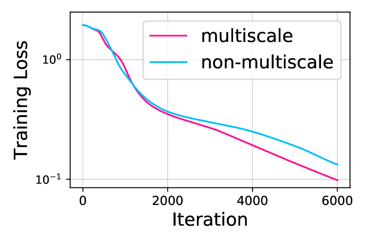
(a) Linear and Cora.

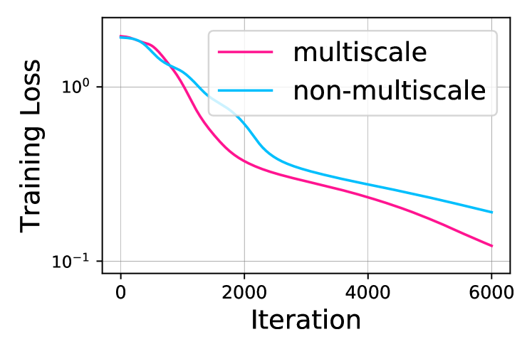
(b) ReLU and Cora.

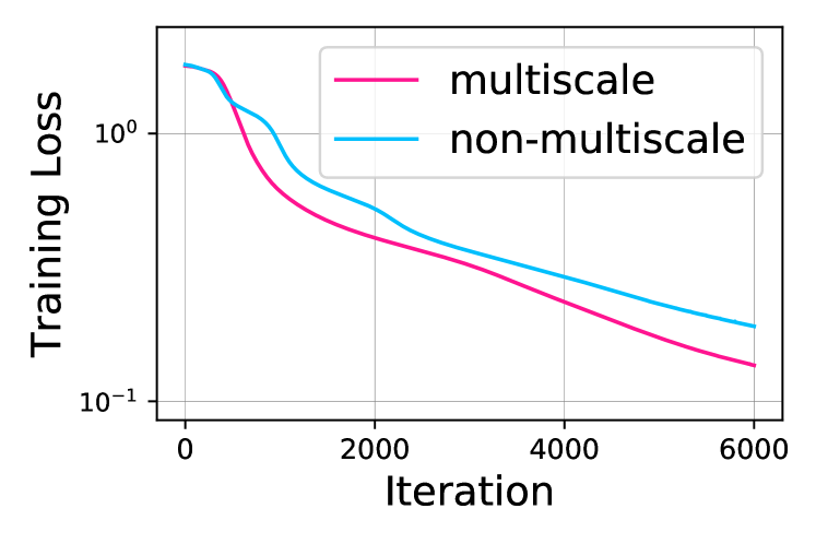
(c) Linear and Citeseer.

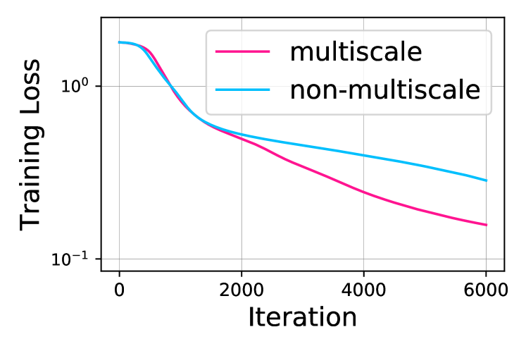
(d) ReLU and Citeseer.

Figure 6: Multiscale skip connection accelerates GNN training. We plot the training curves of GNNs with ReLU and linear activation on the Cora and Citeseer dataset. We use the GCN model with learning rate $5e-5$, six layers, and hidden dimension $32$.

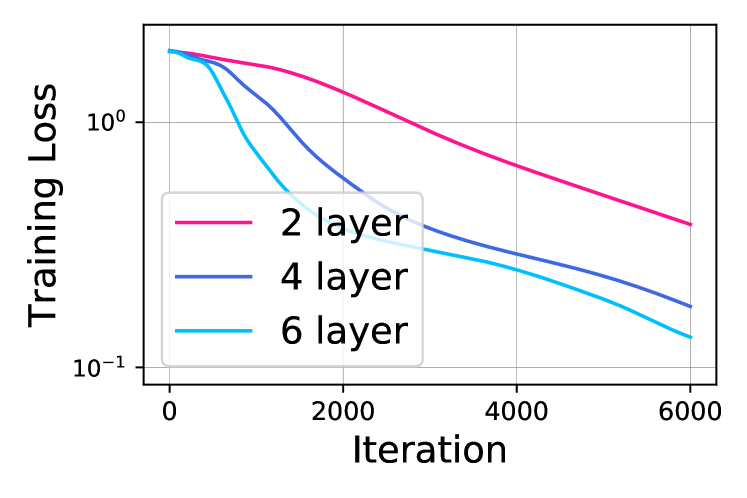
(a) Linear and non-multiscale.

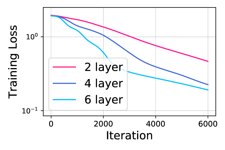
(b) ReLU and non-multiscale.

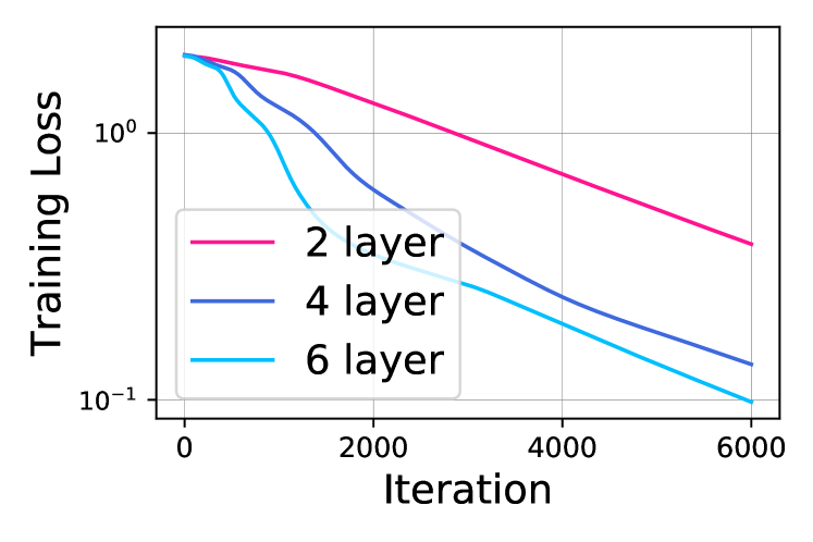
(c) Linear and multiscale.

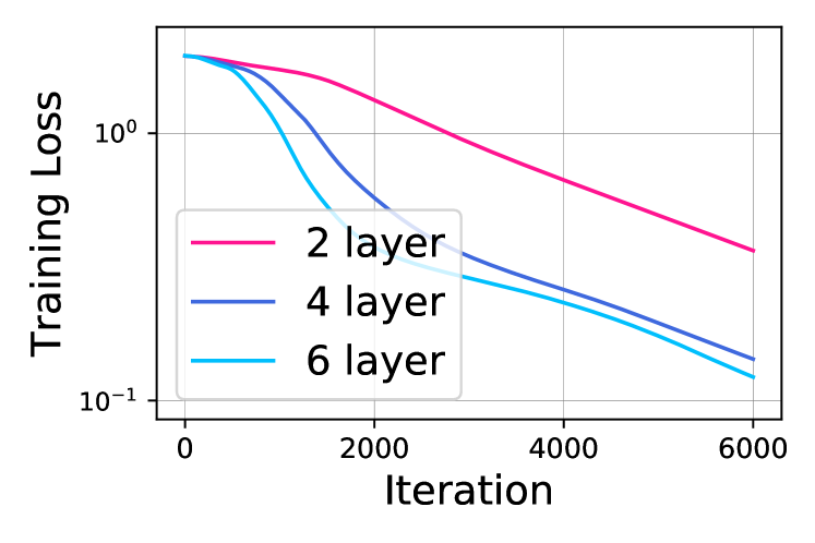
(d) ReLU and multiscale.

Figure 7: Depth accelerates GNN training. We plot the training curves of GNNs with ReLU and linear activation, multiscale and non-multiscale on the Cora dataset. We use the GCN model with learning rate $5e-5$ and hidden dimension $32$.

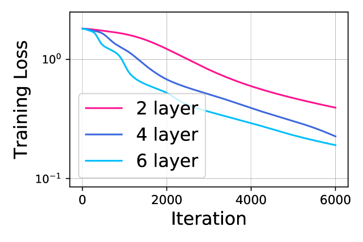
(a) Linear and non-multiscale.

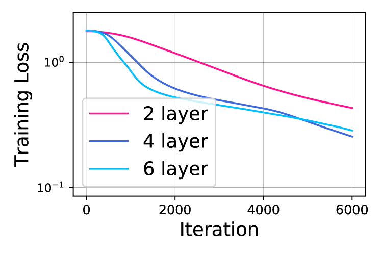
(b) ReLU and non-multiscale.

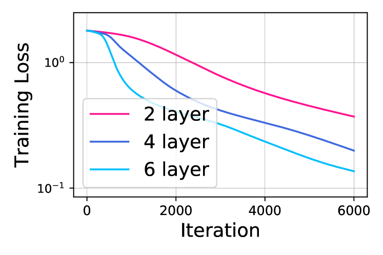
(c) Linear and multiscale.

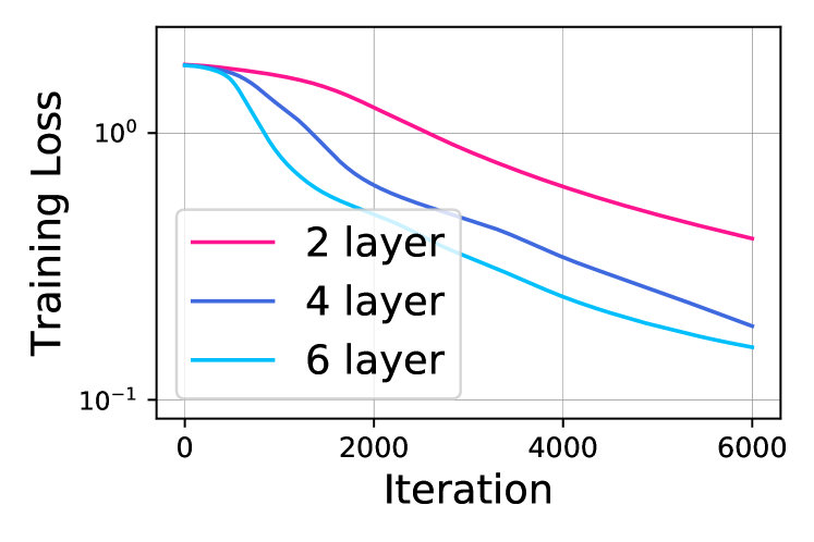
(d) ReLU and multiscale.

Figure 8: Depth accelerates GNN training. We plot the training curves of GNNs with ReLU and linear activation, multiscale and non-multiscale on the Citeseer dataset. We use the GCN model with learning rate $5e-5$ and hidden dimension $32$.

(a) Linear and non-multiscale.

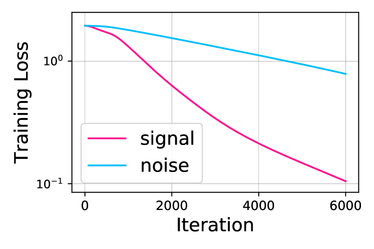
(b) ReLU and non-multiscale.

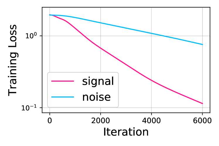
(c) Linear and multiscale.

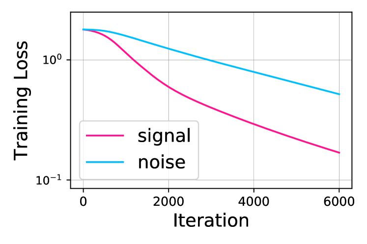
(d) ReLU and multiscale.

Figure 9: GNNs train faster when the labels have signal instead of random noise. We plot the training curves of multiscale and non-multiscale GNNs with ReLU and linear activation, on the Cora dataset. We use the two-layer GCN model with learning rate $1e-4$ and hidden dimension $32$.

(a) Linear and non-multiscale.

(b) ReLU and non-multiscale.

(c) Linear and multiscale.

(d) ReLU and multiscale.

Figure 10: GNNs train faster when the labels have signal instead of random noise. We plot the training curves of multiscale and non-multiscale GNNs with ReLU and linear activation, on the Citeseer dataset. We use the two-layer GCN model with learning rate $1e-4$ and hidden dimension $32$.

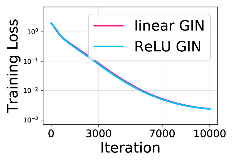
(a) Linear GIN vs. ReLU GIN.

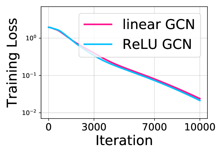
(b) Linear GCN vs. ReLU GCN.

Figure 11: Linear GNNs vs. ReLU GNNs. We plot the training curves of GCN and GIN with ReLU and linear activation on the Cora dataset. The training curves of linear GNNs and ReLU GNNs are similar, both converging to nearly zero training loss with the same linear rate. Moreover, GIN trains faster than GCN, which agrees with our bound in Theorem 1. We use the learning rate $1e-4$, two layers, and hidden dimension $32$.

Appendix C Experimental Setup

In this section, we describe the experimental setup for reproducing our experiments.

Dataset.

We perform all experiments on the Cora and Citeseer datasets (Sen et al., 2008). Cora and Citeer are citation networks and the goal is to classify academic documents into different subjects. The dataset contains bag-of-words features for each document (node) and citation links (edges) between documents. The tasks are semi-supervised node classification. Only a subset of nodes have training labels. In our experiments, we use the default dataset split, i.e., which nodes have training labels, and minimize the training loss accordingly. Tabel 1 shows an overview of the dataset statistics.

Dataset	Nodes	Edges	Classes	Features
Citeseer	3,327	4,732	6	3,703
Cora	2,708	5,429	7	1,433

Table 1: Dataset statistics

Training details.

We describe the training settings for our experiments. Let us first describe some common hyperparameters and settings, and then for each experiment or figure we describe the other hyperparameters. For our experiments, to more closely align with the common practice in GNN training, we use the Adam optimizer and keep optimizer-specific hyperparameters except initial learning rate default. We set weight decay to zero. Next, we describe the settings for each experiment respectively.

For the experiment in Figure 1, i.e., the training curves of linear vs. ReLU GNNs, we train the GCN and GIN with two layers on Cora with cross-entropy loss and learning rate 1e-4. We set the hidden dimension to $32$.

For the experiment in Figure 2(a), i.e., computing the graph condition for linear GNNs, we use the linear GCN and GIN model with three layers on Cora and Citeseer. For linear GIN, we set $\epsilon$ to zero and MLP layer to one.

For the experiment in Figure 2(b), i.e., computing and plotting the time-dependent condition for linear GNNs, we train a linear GCN with two layers on Cora with squared loss and learning rate 1e-4. We set the hidden dimension the input dimension for both Cora and for CiteSeer, because the global convergence theorem requires the hidden dimension to be at least the same as input dimension. Note that this requirement is standard in previous works as well, such as Arora et al. (2019a). We use the default random initialization of PyTorch. The formula for computing the time-dependent $\lambda_{T}$ is given in the main paper.

For the experiment in Figure 2(c), i.e., computing and plotting the time-dependent condition for linear GNNs across multiple training settings, we consider the following settings:

1. Dataset: Cora and Citeseer.

2. Model: GCN and GIN.

3. Depth: Two and four layers.

4. Activation: Linear and ReLU.

We train the GNN with the settings above with squared loss and learning rate 1e-4. We set the hidden dimension to input dimension for Cora and CiteSeer. We use the default random initialization of PyTorch. The formula for computing the time-dependent $\lambda_{T}$ is given in the main paper. For each point, we report the $\lambda_{T}$ at last epoch.

For the experiment in Figure 3(a), i.e., computing the graph condition for multiscale linear GNNs, we use the linear GCN and GIN model with three layers on Cora and Citeseer. For linear GIN, we set $\epsilon$ to zero and MLP layer to one.

For the experiment in Figure 3(b), i.e., computing and plotting the time-dependent condition for multiscale linear GNNs, we train a linear GCN with two layers on Cora with squared loss and learning rate 1e-4. We set the hidden dimension to 2000 for Cora and 4000 for CiteSeer. We use the default random initialization of PyTorch. The formula for computing the time-dependent $\lambda_{T}$ is given in the main paper.

For the experiment in Figure 3(c), i.e., computing and plotting the time-dependent condition for multiscale linear GNNs across multiple training settings, we consider the following settings:

1. Dataset: Cora and Citeseer.

2. Model: Multiscale GCN and GIN.

3. Depth: Two and four layers.

4. Activation: Linear and ReLU.

We train the multiscale GNN with the settings above with squared loss and learning rate 1e-4. We set the hidden dimension to 2000 for Cora and 4000 for CiteSeer. We use the default random initialization of PyTorch. The formula for computing the time-dependent $\lambda_{T}$ is given in the main paper. For each point, we report the $\lambda_{T}$ at last epoch.

For the experiment in Figure 4(a), i.e., multiscale vs. non-multiscale, we train the GCN with six layers and ReLU activation on Cora with cross-entropy loss and learning rate 5e-5. We set the hidden dimension to $32$.

We perform more extensive experiments to verify the conclusion for multiscale vs. non-multiscale in Figure 11. There, we train the GCN with six layers with both ReLU and linear activation on both Cora and Citeseer with cross-entropy loss and learning rate 5e-5. We set the hidden dimension to $32$.

For the experiment in Figure 4(b), i.e., acceleration with depth, we train the non-multiscale GCN with two, four, six layers and ReLU activation on Cora with cross-entropy loss and learning rate 5e-5. We set the hidden dimension to $32$.

We perform more extensive experiments to verify the conclusion for acceleration with depth in Figure 7 and Figure 8. There, we train both multiscale and non-multiscale GCN with $2$, $4$, $6$ layers with both ReLU and linear activation on both Cora and Citeseer with cross-entropy loss and learning rate 5e-5. We set the hidden dimension to $32$.

For the experiment in Figure 4(c), i.e., signal vs. noise, we train the non-multiscale GCN with two layers and ReLU activation on Cora with cross-entropy loss and learning rate 1e-4. We set the hidden dimension to $32$. For signal, we use the default labels of Cora. For noise, we randomly choose a class as the label.

We perform more extensive experiments to verify the conclusion for signal vs. noise in Figure 9 and Figure 10. There, we train both multiscale and non-multiscale GCN with two layers with both ReLU and linear activation on both Cora and Citeseer with cross-entropy loss and learning rate 1e-4. We set the hidden dimension to $32$.

For the experiment in Figure 5, i.e., first term vs. second term, we use the same setting as in Figure 4(c). We use the formula of our Theorem in the main paper.

Computing resources.

The computing hardware is based on the CPU and the NVIDIA GeForce RTX 1080 Ti GPU. The software implementation is based on PyTorch and PyTorch Geometric (Fey & Lenssen, 2019). For all experiments, we train the GNNs with CPU and compute the eigenvalues with GPU.

References

- Abu-El-Haija et al. (2020) Abu-El-Haija, S., Kapoor, A., Perozzi, B., and Lee, J. N-gcn: Multi-scale graph convolution for semi-supervised node classification. In Uncertainty in Artificial Intelligence, pp. 841–851. PMLR, 2020.
- Allen-Zhu et al. (2019) Allen-Zhu, Z., Li, Y., and Song, Z. A convergence theory for deep learning via over-parameterization. In International Conference on Machine Learning, pp. 242–252, 2019.
- Arora et al. (2018) Arora, S., Cohen, N., and Hazan, E. On the optimization of deep networks: Implicit acceleration by overparameterization. In International Conference on Machine Learning, pp. 244–253. PMLR, 2018.
- Arora et al. (2019a) Arora, S., Cohen, N., Golowich, N., and Hu, W. A convergence analysis of gradient descent for deep linear neural networks. In International Conference on Learning Representations, 2019a.
- Arora et al. (2019b) Arora, S., Du, S., Hu, W., Li, Z., and Wang, R. Fine-grained analysis of optimization and generalization for overparameterized two-layer neural networks. In International Conference on Machine Learning, pp. 322–332, 2019b.
- Bartlett et al. (2019) Bartlett, P. L., Helmbold, D. P., and Long, P. M. Gradient descent with identity initialization efficiently learns positive-definite linear transformations by deep residual networks. Neural computation, 31(3):477–502, 2019.
- Cai et al. (2020) Cai, T., Luo, S., Xu, K., He, D., Liu, T.-y., and Wang, L. Graphnorm: A principled approach to accelerating graph neural network training. arXiv preprint arXiv:2009.03294, 2020.
- Chen et al. (2018a) Chen, J., Ma, T., and Xiao, C. FastGCN: Fast learning with graph convolutional networks via importance sampling. In International Conference on Learning Representations, 2018a.
- Chen et al. (2018b) Chen, J., Zhu, J., and Song, L. Stochastic training of graph convolutional networks with variance reduction. In International Conference on Machine Learning, pp. 942–950, 2018b.
- Chen et al. (2020) Chen, M., Wei, Z., Huang, Z., Ding, B., and Li, Y. Simple and deep graph convolutional networks. In International Conference on Machine Learning, pp. 1725–1735. PMLR, 2020.
- Chen et al. (2019) Chen, Z., Villar, S., Chen, L., and Bruna, J. On the equivalence between graph isomorphism testing and function approximation with gnns. In Advances in Neural Information Processing Systems, pp. 15894–15902, 2019.
- Chiang et al. (2019) Chiang, W.-L., Liu, X., Si, S., Li, Y., Bengio, S., and Hsieh, C.-J. Cluster-gcn: An efficient algorithm for training deep and large graph convolutional networks. In Proceedings of the 25th ACM SIGKDD International Conference on Knowledge Discovery & Data Mining, pp. 257–266, 2019.
- Chizat et al. (2019) Chizat, L., Oyallon, E., and Bach, F. On lazy training in differentiable programming. In Advances in Neural Information Processing Systems, pp. 2937–2947, 2019.
- Defferrard et al. (2016) Defferrard, M., Bresson, X., and Vandergheynst, P. Convolutional neural networks on graphs with fast localized spectral filtering. In Advances in Neural Information Processing Systems, pp. 3844–3852, 2016.
- Du & Hu (2019) Du, S. and Hu, W. Width provably matters in optimization for deep linear neural networks. In International Conference on Machine Learning, pp. 1655–1664, 2019.
- Du et al. (2019a) Du, S., Lee, J., Li, H., Wang, L., and Zhai, X. Gradient descent finds global minima of deep neural networks. In International Conference on Machine Learning, pp. 1675–1685, 2019a.
- Du et al. (2019b) Du, S. S., Hou, K., Salakhutdinov, R. R., Poczos, B., Wang, R., and Xu, K. Graph neural tangent kernel: Fusing graph neural networks with graph kernels. In Advances in Neural Information Processing Systems, pp. 5724–5734, 2019b.
- Du et al. (2019c) Du, S. S., Zhai, X., Poczos, B., and Singh, A. Gradient descent provably optimizes over-parameterized neural networks. In International Conference on Learning Representations, 2019c.
- Duvenaud et al. (2015) Duvenaud, D. K., Maclaurin, D., Iparraguirre, J., Bombarell, R., Hirzel, T., Aspuru-Guzik, A., and Adams, R. P. Convolutional networks on graphs for learning molecular fingerprints. In Advances in neural information processing systems, pp. 2224–2232, 2015.
- Fey & Lenssen (2019) Fey, M. and Lenssen, J. E. Fast graph representation learning with pytorch geometric. arXiv preprint arXiv:1903.02428, 2019.
- Garg et al. (2020) Garg, V. K., Jegelka, S., and Jaakkola, T. Generalization and representational limits of graph neural networks. In International Conference on Machine Learning, 2020.
- Gilmer et al. (2017) Gilmer, J., Schoenholz, S. S., Riley, P. F., Vinyals, O., and Dahl, G. E. Neural message passing for quantum chemistry. In International Conference on Machine Learning, pp. 1273–1272, 2017.
- Gori et al. (2005) Gori, M., Monfardini, G., and Scarselli, F. A new model for learning in graph domains. In Proceedings. 2005 IEEE International Joint Conference on Neural Networks, 2005., volume 2, pp. 729–734. IEEE, 2005.
- Hamilton et al. (2017) Hamilton, W. L., Ying, R., and Leskovec, J. Inductive representation learning on large graphs. In Advances in Neural Information Processing Systems, pp. 1025–1035, 2017.
- Hardt & Ma (2017) Hardt, M. and Ma, T. Identity matters in deep learning. In International Conference on Learning Representations, 2017.
- Huang & Yau (2020) Huang, J. and Yau, H.-T. Dynamics of deep neural networks and neural tangent hierarchy. In International conference on machine learning, 2020.
- Huang et al. (2018) Huang, W., Zhang, T., Rong, Y., and Huang, J. Adaptive sampling towards fast graph representation learning. Advances in neural information processing systems, 31:4558–4567, 2018.
- Jacot et al. (2018) Jacot, A., Gabriel, F., and Hongler, C. Neural tangent kernel: Convergence and generalization in neural networks. In Advances in neural information processing systems, pp. 8571–8580, 2018.
- Ji & Telgarsky (2020) Ji, Z. and Telgarsky, M. Directional convergence and alignment in deep learning. arXiv preprint arXiv:2006.06657, 2020.
- Kawaguchi (2016) Kawaguchi, K. Deep learning without poor local minima. In Advances in Neural Information Processing Systems, pp. 586–594, 2016.
- Kawaguchi (2021) Kawaguchi, K. On the theory of implicit deep learning: Global convergence with implicit layers. In International Conference on Learning Representations (ICLR), 2021.
- Kawaguchi & Huang (2019) Kawaguchi, K. and Huang, J. Gradient descent finds global minima for generalizable deep neural networks of practical sizes. In 2019 57th Annual Allerton Conference on Communication, Control, and Computing (Allerton), pp. 92–99. IEEE, 2019.
- Kearnes et al. (2016) Kearnes, S., McCloskey, K., Berndl, M., Pande, V., and Riley, P. Molecular graph convolutions: moving beyond fingerprints. Journal of computer-aided molecular design, 30(8):595–608, 2016.
- Keriven & Peyré (2019) Keriven, N. and Peyré, G. Universal invariant and equivariant graph neural networks. In Advances in Neural Information Processing Systems, pp. 7092–7101, 2019.
- Kipf & Welling (2017) Kipf, T. N. and Welling, M. Semi-supervised classification with graph convolutional networks. In International Conference on Learning Representations, 2017.
- Laurent & Brecht (2018) Laurent, T. and Brecht, J. Deep linear networks with arbitrary loss: All local minima are global. In International conference on machine learning, pp. 2902–2907. PMLR, 2018.
- Lee et al. (2019) Lee, J., Xiao, L., Schoenholz, S., Bahri, Y., Novak, R., Sohl-Dickstein, J., and Pennington, J. Wide neural networks of any depth evolve as linear models under gradient descent. In Advances in neural information processing systems, pp. 8572–8583, 2019.
- Li et al. (2019) Li, G., Muller, M., Thabet, A., and Ghanem, B. Deepgcns: Can gcns go as deep as cnns? In Proceedings of the IEEE International Conference on Computer Vision, pp. 9267–9276, 2019.
- Li et al. (2020) Li, G., Xiong, C., Thabet, A., and Ghanem, B. Deepergcn: All you need to train deeper gcns. arXiv preprint arXiv:2006.07739, 2020.
- Li & Liang (2018) Li, Y. and Liang, Y. Learning overparameterized neural networks via stochastic gradient descent on structured data. In Advances in Neural Information Processing Systems, pp. 8157–8166, 2018.
- Liao et al. (2020) Liao, P., Zhao, H., Xu, K., Jaakkola, T., Gordon, G., Jegelka, S., and Salakhutdinov, R. Graph adversarial networks: Protecting information against adversarial attacks. arXiv preprint arXiv:2009.13504, 2020.
- Liu et al. (2020) Liu, C., Zhu, L., and Belkin, M. On the linearity of large non-linear models: when and why the tangent kernel is constant. Advances in Neural Information Processing Systems, 33, 2020.
- Loukas (2020) Loukas, A. How hard is to distinguish graphs with graph neural networks? In Advances in neural information processing systems, 2020.
- Maron et al. (2019) Maron, H., Ben-Hamu, H., Serviansky, H., and Lipman, Y. Provably powerful graph networks. In Advances in Neural Information Processing Systems, pp. 2156–2167, 2019.
- Merkwirth & Lengauer (2005) Merkwirth, C. and Lengauer, T. Automatic generation of complementary descriptors with molecular graph networks. J. Chem. Inf. Model., 45(5):1159–1168, 2005.
- Nitanda & Suzuki (2021) Nitanda, A. and Suzuki, T. Optimal rates for averaged stochastic gradient descent under neural tangent kernel regime. In International Conference on Learning Representations, 2021.
- Oono & Suzuki (2020) Oono, K. and Suzuki, T. Optimization and generalization analysis of transduction through gradient boosting and application to multi-scale graph neural networks. Advances in Neural Information Processing Systems, 33, 2020.
- Sato et al. (2019) Sato, R., Yamada, M., and Kashima, H. Approximation ratios of graph neural networks for combinatorial problems. In Advances in Neural Information Processing Systems, pp. 4083–4092, 2019.
- Sato et al. (2020) Sato, R., Yamada, M., and Kashima, H. Random features strengthen graph neural networks. arXiv preprint arXiv:2002.03155, 2020.
- Saxe et al. (2014) Saxe, A. M., McClelland, J. L., and Ganguli, S. Exact solutions to the nonlinear dynamics of learning in deep linear neural networks. In International Conference on Learning Representations, 2014.
- Scarselli et al. (2009) Scarselli, F., Gori, M., Tsoi, A. C., Hagenbuchner, M., and Monfardini, G. The graph neural network model. IEEE Transactions on Neural Networks, 20(1):61–80, 2009.
- Scarselli et al. (2018) Scarselli, F., Tsoi, A. C., and Hagenbuchner, M. The vapnik–chervonenkis dimension of graph and recursive neural networks. Neural Networks, 108:248–259, 2018.
- Sen et al. (2008) Sen, P., Namata, G., Bilgic, M., Getoor, L., Galligher, B., and Eliassi-Rad, T. Collective classification in network data. AI magazine, 29(3):93, 2008.
- Thekumparampil et al. (2018) Thekumparampil, K. K., Wang, C., Oh, S., and Li, L.-J. Attention-based graph neural network for semi-supervised learning. arXiv preprint arXiv:1803.03735, 2018.
- Velickovic et al. (2018) Velickovic, P., Cucurull, G., Casanova, A., Romero, A., Lio, P., and Bengio, Y. Graph attention networks. In International Conference on Learning Representations, 2018.
- Vignac et al. (2020) Vignac, C., Loukas, A., and Frossard, P. Building powerful and equivariant graph neural networks with message-passing. Advances in neural information processing systems, 2020.
- Wu et al. (2019) Wu, F., Souza, A., Fifty, C., Yu, T., and Weinberger, K. Simplifying graph convolutional networks. In International Conference on Machine Learning, 2019.
- Xu et al. (2018) Xu, K., Li, C., Tian, Y., Sonobe, T., Kawarabayashi, K.-i., and Jegelka, S. Representation learning on graphs with jumping knowledge networks. In International Conference on Machine Learning, pp. 5453–5462, 2018.
- Xu et al. (2019) Xu, K., Hu, W., Leskovec, J., and Jegelka, S. How powerful are graph neural networks? In International Conference on Learning Representations, 2019.
- Xu et al. (2020) Xu, K., Li, J., Zhang, M., Du, S. S., ichi Kawarabayashi, K., and Jegelka, S. What can neural networks reason about? In International Conference on Learning Representations, 2020.
- Xu et al. (2021) Xu, K., Zhang, M., Li, J., Du, S. S., Kawarabayashi, K.-I., and Jegelka, S. How neural networks extrapolate: From feedforward to graph neural networks. In International Conference on Learning Representations, 2021.
- Yehudai & Shamir (2019) Yehudai, G. and Shamir, O. On the power and limitations of random features for understanding neural networks. In Advances in Neural Information Processing Systems, pp. 6598–6608, 2019.
- Zhang et al. (2020) Zhang, S., Wang, M., Liu, S., Chen, P.-Y., and Xiong, J. Fast learning of graph neural networks with guaranteed generalizability: One-hidden-layer case. In International Conference on Machine Learning, pp. 11268–11277, 2020.
- Zou et al. (2019) Zou, D., Hu, Z., Wang, Y., Jiang, S., Sun, Y., and Gu, Q. Layer-dependent importance sampling for training deep and large graph convolutional networks. In Advances in Neural Information Processing Systems, pp. 11249–11259, 2019.
- Zou et al. (2020) Zou, D., Long, P. M., and Gu, Q. On the global convergence of training deep linear resnets. In International Conference on Learning Representations, 2020.