Learning High-Dimensional Distributions with
Latent Neural Fokker-Planck Kernels

Abstract

Learning high-dimensional distributions is an important yet challenging problem in machine learning with applications in various domains. In this paper, we introduce new techniques to formulate the problem as solving Fokker-Planck equation in a lower-dimensional latent space, aiming to mitigate challenges in high-dimensional data space. Our proposed model consists of latent-distribution morphing, a generator and a parameterized Fokker-Planck kernel function. One fascinating property of our model is that it can be trained with arbitrary steps of latent distribution morphing or even without morphing, which makes it flexible and as efficient as Generative Adversarial Networks (GANs). Furthermore, this property also makes our latent-distribution morphing an efficient plug-and-play scheme, thus can be used to improve arbitrary GANs, and more interestingly, can effectively correct failure cases of the GAN models. Extensive experiments illustrate the advantages of our proposed method over existing models.

1 Introduction

Learning a complex distribution from high-dimensional data is an important and challenging problem in machine learning with a variety of real-world applications such as synthesizing high-fidelity data. Some representative approaches for solving this problem include generative adversarial networks (GANs) (Goodfellow et al., 2014), variational auto-encoder (VAEs) (Kingma & Welling, 2014), normalizing flows (Rezende & Mohamed, 2015; Kingma & Dhariwal, 2018), enegy-based models (EBMs) (Du & Mordatch, 2019), etc. Despite their tremendous successes, each of them also suffers from its own intrinsic limitations which are partially caused by the complex nature of the high-dimensional data space.

GAN (Goodfellow et al., 2014) is perhaps one of the most popular generative models due to its ability to generate high-fidelity data. In recent years, there has been a surge of interest in developing various types of GANs by designing new objectives (Li et al., 2017; Arjovsky et al., 2017; Genevay et al., 2018; Wang et al., 2018) or stabilizing the training process (Miyato et al., 2018; Gulrajani et al., 2017; Arbel et al., 2018). A common and well-known issue of all such GANs is the seemingly unavoidable mode collapse. We conjecture that this is partially due to the following two reasons: 1) GAN directly optimizes its objective function in the often complicated high-dimensional data space, and thus is more likely to get stuck at some sub-optimal solutions; and 2) GAN aims to learn a mapping from a flat and single-mode latent distribution (e.g., Gaussian) to a complex, high dimensional and possibly multi-mode data distribution. This complicated mapping could impose a tremendous challenge to learn all modes in the optimization process.

VAE and Normalizing Flow based methods are likelihood-driven models, making them more tractable but potentially less expressive compared to GANs. A consequence is that the generated data from these models are smoother and less real-looking. EBM assumes that the data distribution follows an unnormalized energy-based form, making it more tractable than GANs and more flexible than VAEs. However, its training requires samples generated from the model distribution, which is typically done via Langevin dynamics (Roberts et al., 1996; Welling & Teh, 2011), which could be time-consuming in practice and could suffer considerably from the high domensionality of the data space. Recently, some works have been proposed to alleviate this problem, by combining a generator with the EBM (Kumar et al., 2019; Grathowhl et al., 2020; Xie et al., 2020; Arbel et al., 2020), we will discuss the major difference between our proposed method with theirs and provide experimental comparisons in later sections.

To deal with the aforementioned issues, we propose, in this paper, a new framework to learn the implicit distribution of high dimensional data via deep generative models (DGMs). Our framework aims to achieve the following goals: 1) define the problem in the space of probability measure and avoid learning the complicated and possibly single-to-multi-mode matching from the latent space to the data space as in GAN; and 2) relieve from the requirement of sampling from data space for learning as in EBM. To realize these goals,

• we formulate the problem of learning high-dimensional distribution as one that learns a neural Fokker-Planck kernel, inspired by the Fokker-Planck (FP) equation (Risken, 1996);

• we define the Fokker-Planck kernel in a much lower dimensional latent space so that learning becomes morphing a flat latent distribution into a more complex one in the same latent space. Consequently, mapping from the latent space to the data space is carried out by a multi-mode distribution matching scheme, implemented by a parameterized generator.

In summary, our framework consists of three components: 1) a parameterized kernel function representing the FP kernel; 2) a latent-distribution morphing scheme implemented via gradient flows in the latent space; and 3) a generator mapping samples in the latent space to samples in the data space. The connection between the three components is illustrated in Figure 1. A remarkable feature of our framework is that the latent-distribution morphing scheme allows us to develop a plug-and-play mechanism directly from pre-trained GAN models, where we use our latent-distribution morphing scheme to optimize their flat latent distributions. This gives us a fine-tuning mechanism independent of the original GAN models, which can lead to significant improvement over the original GANs. In experiments, we show that our latent-distribution morphing scheme can be used to mitigate the mode collapses problem, indicating that mode collapse is indeed partially caused by the mis-matching between the simple latent distribution and the complex data distribution. Moreover, based on a number of state-of-the-art architecture settings and extensive experiments, we demonstrate the advantages of our proposed framework over existing models on a number of tasks, including high-fidelity image generation and image translation.

2 The Proposed Framework

In this paper, we follow the commonly adopted assumption that the observed data are sampled from a lower-dimensional manifold embedded in the high-dimensional space. Let $\mathcal{Z}$ be the low-dimensional latent space, $\mathcal{X}$ be the data space, and $g:\mathcal{Z}\rightarrow\mathcal{X}$ be a mapping from the latent representations to data samples. Let $p(\operatorname{\mathbf{z}}),q(\operatorname{\mathbf{z}}),\operatorname{\mathbf{z}}\in\mathcal{Z}$, be two distributions in the latent space, and $P(\operatorname{\mathbf{x}})$ and $Q(\operatorname{\mathbf{x}})$, $\operatorname{\mathbf{x}}\in\mathcal{X}$, be their corresponding distributions in the data space induced by the mapping $g$ ($g$ is also called the generator).

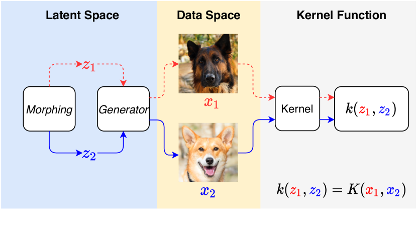
Figure 1: An overview of the proposed framework. The key components include a latent-distribution morphing mechanism, a parameterized generator and a neural Fokker-Planck kernel.

Assume that $P$ is the target distribution to be learned from a set of observed data. Instead of directly learning $P$, we propose to learn its associated latent distribution $p$ first. To this end, by the variational principle, we will learn a distribution $q$ such that it is close to $p$ under some metric. A natural way to obtain $q$ is to formulate the problem in $\mathcal{P}_{2}$, the space of probability measures endowed with the 2-Wasserstein distance (Santambrogio, 2016), as:

$$q^{*}=\arg\min_{q\in\mathcal{P}_{2}}F(q,p)~{},$$ (1)

where $F(q,p)$ is a functional measuring the difference between $p$ and $q$. A popular choice of $F$ is the KL-divergence, which would make (1) equivalent to maximizing the negative log-likelihood $-\mathbb{E}_{p(\operatorname{\mathbf{z}})}\left[\log(q(\operatorname{\mathbf{z}}))\right]$. For a more general setting, we instead focus on the $f$-divergence $D_{f}(p_{D}\|q)$, defined as

$$D_{f}(p\|q)=\int_{\mathcal{Z}}q(\operatorname{\mathbf{z}})f(p(\operatorname{\mathbf{z}})/q(\operatorname{\mathbf{z}}))\text{d}\operatorname{\mathbf{z}}~{},$$

where $f:(0,\infty)\rightarrow R$ is a convex function with $f(1)=0$. Many distribution metrics are special cases of $f$-divergence, including the Kullback-Leibler (KL) divergence and the Jensen-Shannon (JS) divergence. An important property of $f$-divergence is its convexity, i.e., $p\rightarrow D_{f}(p\|q)$ and $q\rightarrow D_{f}(p\|q)$ are both convex.

Default solutions via Wasserstein gradient flows (WGFs)

With the convexity of the $f$-divergence, a default solution to problem (1) is by applying the method of WGF (Ambrosio et al., 2008; Santambrogio, 2016). Specifically, (1) is re-written as a WGF in the space of probability measures, which is represented by a partial differential equation (PDE):

$$\dfrac{\partial q}{\partial t}=-\nabla_{W_{2}}F(q,p)\triangleq-\nabla_{W_{2}}D_{f}(p\|q)~{},$$ (2)

The following lemma ensures the convergence of the $f$-divergence under WGF.

Lemma 1

Assume that $(q^{t})_{t\geq 0}$ evolves according to the WGF of $f$-divergence, $F(q^{t},p)=D_{f}(p\|q^{t})$, with initialization $q^{0}$. Let $d_{W_{2}}(\cdot,\cdot)$ be the 2-Wasserstein distance. Assume that $F(q^{0},p)<\infty$ and $d_{W_{2}}(q^{0},p)<\infty$. Then, the following holds:
1) $F(q^{t},p)$ is non-increasing and converges to the global optimum as $t\rightarrow\infty$;
2) If $\|\nabla_{W_{2}}F(q^{t},p)\|^{2}\geq\lambda F(q^{t},p)$ with some constant $\lambda>0$, then $F(q^{t},p)\leq\exp(-\lambda t)F(q^{0},p)$;
3) If $F(q^{t},p)$ is $\lambda$-geodesically convex with some constant $\lambda>0$, then $d_{W_{2}}(q^{t},p)\leq\exp(-\lambda t)d_{W_{2}}(q^{0},p)$;
4) If mapping $g$ is Lipschitz continuous, then $d_{W_{2}}(Q^{t},P)$ converges with the same convergence rate as $d_{W_{2}}(q^{t},p)$.

To solve the WGF problem (2), a popular way is to use the Jordan-Kinderlehrer-Otto (JKO) scheme (Jordan et al., 1998), which derive the solution of the PDE via solving a sequence of optimization problems: $q^{k+1}(\operatorname{\mathbf{z}})=\operatorname*{arg\,min}_{q}D_{f}(p\|q)+d^{2}_{W_{2}}(q^{k},q)/(2h)$, where $k=0,1,2...$, $h$ is a hyper-parameter. In practice, $d^{2}_{W}$ is computationally infeasible, and thus can be approximated with different methods (Cuturi, 2013; Chizat et al., 2020). However, a potential issue of previous works using this method is that optimization is performed directly on the high-dimensional data space, which could be severely impacted by the curse of dimensionality.

2.1 Reformulation with Latent Neural FP Kernels

It is known that $\nabla_{W_{2}}F(q,p)=-div(q\nabla_{\operatorname{\mathbf{z}}}\delta F/\delta q)$ (Santambrogio, 2016), where $\delta F/\delta q$ denotes the first variation of functional $F$ at $q$, and $div$ denotes the divergence operator. With this, we can re-write (2) as:

$$\dfrac{\partial q}{\partial t}=div(q\nabla_{\operatorname{\mathbf{z}}}\psi(\operatorname{\mathbf{z}})),\text{where }\psi(\operatorname{\mathbf{z}})=\dfrac{\delta D_{f}(p\|q)}{\delta q}~{}.$$ (3)

(3) is a special case of the well-known FP equation. In the following, we propose a kernel based parameterization inspired by the FP kernel (Risken, 1996; Carrillo & Toscani, 1998; Bilal, 2020) to solve (3). One advantage of the FP kernel is that it can be solved efficiently with simple and mesh-free methods, which can be applied on irregular and complicated spaces.

Following (Bilal, 2020), we denote the FP kernel as $k(t,\operatorname{\mathbf{x}},s,\operatorname{\mathbf{y}})$, with $t$ and $s$ being the time indexes. For the FP equation (3), the theory of FP kernels reveals that the density function $q^{t}(\operatorname{\mathbf{z}})$ at any time $t$ is characterized by a convolutional form as (Bilal, 2020):

$$q^{t}(\operatorname{\mathbf{z}})=\int_{\mathcal{Z}}k(t,\operatorname{\mathbf{z}},s,\operatorname{\mathbf{z}}^{\prime})q^{s}(\operatorname{\mathbf{z}}^{\prime})\exp(V^{s}(\operatorname{\mathbf{z}}^{\prime}))\text{d}\operatorname{\mathbf{z}}^{\prime}~{},$$ (4)

where $V$ is an arbitrary priori function, and $s$ indexes arbitrary time. According to Lemma 1, we expect $q(\operatorname{\mathbf{z}})$ to converge to $p(\operatorname{\mathbf{z}})$ at the infinite-time limit, i.e., $q^{\infty}(\operatorname{\mathbf{z}})=p(\operatorname{\mathbf{z}})$. Consequently, taking $s\rightarrow\infty$ in (4), our implicit latent distribution $q(\operatorname{\mathbf{z}})$ can be written as

$$q(\operatorname{\mathbf{z}})=\dfrac{\int_{\mathcal{Z}}k(\operatorname{\mathbf{z}},\operatorname{\mathbf{z}}^{\prime})p(\operatorname{\mathbf{z}}^{\prime})\text{d}\operatorname{\mathbf{z}}^{\prime}}{Z}\triangleq\dfrac{\tilde{q}(\operatorname{\mathbf{z}})}{Z},$$

where $Z=\int\tilde{q}(\operatorname{\mathbf{x}})d\operatorname{\mathbf{x}}$ is the normalizer, and the $V$ function in (4) has been defined as a special constant function. Furthermore, we will not directly describe the dependency of $k$ on $t$ in the following as it corresponds to the optimization process. Due to the fact that we have access only to the real samples in the data space but not in the latent space, we propose to construct a deep kernel via the generator $g$ as $k=K\circ g$ with $K$ being a kernel function in the data space:

$$k(\operatorname{\mathbf{z}},\operatorname{\mathbf{z}}^{\prime})=K(g(\operatorname{\mathbf{z}}),g(\operatorname{\mathbf{z}}^{\prime}))=K(g(\operatorname{\mathbf{z}}),\operatorname{\mathbf{x}}^{\prime})~{},$$ (5)

where $\operatorname{\mathbf{x}}^{\prime}$ corresponds to a training data sample from $P(\operatorname{\mathbf{x}}^{\prime})$. We will construct $K$ to be a deep kernel (see (7) below) to mitigate challenges in the high-dimensional data space. With such as kernel construction, $q(\operatorname{\mathbf{z}})$ can be written as

$$q(\operatorname{\mathbf{z}})=\dfrac{\mathbb{E}_{P(\operatorname{\mathbf{x}}^{\prime})}\left[K(g(\operatorname{\mathbf{z}}),\operatorname{\mathbf{x}}^{\prime})\right]}{Z}~{}.$$ (6)

Remark 2

Our parameterization (6) is related to EBM (Du & Mordatch, 2019). To see this, re-write our parameterization as $q(\operatorname{\mathbf{z}})\propto\exp(\log\mathbb{E}_{P(\operatorname{\mathbf{x}}^{\prime})}\left[K(g(\operatorname{\mathbf{z}}),\operatorname{\mathbf{x}}^{\prime})\right])$. An EBM defined in the latent space with the form $q(\operatorname{\mathbf{z}})\propto\exp(-E(\operatorname{\mathbf{z}}))$ is recovered if the energy function $E$ is defined as $E(\operatorname{\mathbf{z}})\triangleq-\log\mathbb{E}_{P(\operatorname{\mathbf{x}}^{\prime})}\left[K(g(\operatorname{\mathbf{z}}),\operatorname{\mathbf{x}}^{\prime})\right]$ in the latent space.

In practice, we parameterize $k$ and $g$ with neural networks, written as $f_{\boldsymbol{\phi}}$ and $g_{{\bm{\theta}}}$ with parameters $\boldsymbol{\phi}$ and ${\bm{\theta}}$, respectively. This leads to re-writing (5) as

$$k_{\boldsymbol{\phi},{\bm{\theta}}}(\operatorname{\mathbf{z}},\operatorname{\mathbf{z}}^{\prime})=K_{\boldsymbol{\phi}}(\operatorname{\mathbf{x}},\operatorname{\mathbf{x}}^{\prime})=\exp(-\|f_{\boldsymbol{\phi}}(\operatorname{\mathbf{x}})-f_{\boldsymbol{\phi}}(\operatorname{\mathbf{x}}^{\prime})\|^{2}),$$ (7)

where $\operatorname{\mathbf{z}}\sim q(\operatorname{\mathbf{z}}),\operatorname{\mathbf{z}}^{\prime}\sim p(\operatorname{\mathbf{z}}^{\prime}),\operatorname{\mathbf{x}}=g_{{\bm{\theta}}}(\operatorname{\mathbf{z}})$, and $\operatorname{\mathbf{x}}^{\prime}$ is the data sample corresponding to latent code $\operatorname{\mathbf{z}}^{\prime}$. Note that $K$ and $k$ are valid, positive semi-definite kernels (Shawe-Taylor et al., 2004; Li et al., 2017) by construction. There are other methods to construct potentially more expressive kernels (Rahimi & Recht, 2007; Samo & Roberts, 2015; Remes et al., 2017; Li et al., 2019; Zhou et al., 2019). For simiplicity, we only consider the parameterization in (7).

2.2 Latent-Distribution Morphing

We now discuss how to generate latent codes following $q(\operatorname{\mathbf{z}})$. Starting from a simple latent distribution, we define a new WGF in the latent space whose stationary solution is $q(\operatorname{\mathbf{z}})$. With this, morphing the latent distribution corresponds to solving the WGF to make it converge to $q(\operatorname{\mathbf{z}})$. We implement this by deriving particle update rules for each latent code $\operatorname{\mathbf{z}}$.

Specifically, let $r(\operatorname{\mathbf{z}})$ be the distribution to be updated, implemented by minimizing the $f$-divergence $D_{f}(r\|q)$. This corresponds to the following WGF:

$$\dfrac{\partial r}{\partial t}=-\nabla_{W_{2}}D_{f}(r\|q)=div(r\nabla_{\operatorname{\mathbf{z}}}\dfrac{\delta D_{f}(r\|q)}{\delta r})~{}.$$ (8)

According to (Itô, 1951; Risken, 1996), the corresponding particle optimization can be described by the following ordinary differential equation (ODE):

$$\text{d}\operatorname{\mathbf{z}}=-\nabla_{\operatorname{\mathbf{z}}}\dfrac{\delta D_{f}(r\|q)}{\delta r}\text{d}t~{}.$$ (9)

Note that this WGF (8) is different from (3), which has a different ”target distribution” $q(\operatorname{\mathbf{z}})$ instead of $p(\operatorname{\mathbf{z}})$. We propose to use kernel density estimator (Wasserman, 2006) to estimate $r(\operatorname{\mathbf{z}})$, i.e., $r(\operatorname{\mathbf{z}})=\mathbb{E}_{r(\operatorname{\mathbf{z}}^{\prime})}\left[K_{\boldsymbol{\phi}}(g_{{\bm{\theta}}}(\operatorname{\mathbf{z}}),g_{{\bm{\theta}}}(\operatorname{\mathbf{z}}^{\prime}))\right]\approx\sum_{i=1}^{n}K_{\boldsymbol{\phi}}(g_{{\bm{\theta}}}(\operatorname{\mathbf{z}}),g_{{\bm{\theta}}}(\operatorname{\mathbf{z}}^{\prime}_{i}))/n$. We solve $\operatorname{\mathbf{z}}$ iteratively by substituting the above $r(\operatorname{\mathbf{z}})$ into ODE (9). Using superscript $m$ to index the iteration number and solving (9) result in

$$\operatorname{\mathbf{z}}^{m+1}=\operatorname{\mathbf{z}}^{m}-\lambda\nabla_{\operatorname{\mathbf{z}}}\dfrac{\delta D_{f}(r\|q)}{\delta r},$$ (10)

where $\lambda$ is the step size; and $\operatorname{\mathbf{z}}^{0}\sim\text{Uniform}\left[-1,1\right]^{dim(\operatorname{\mathbf{z}})}$. We consider different forms of $D_{f}$, including reverse Kullback-Leibler (RKL), Jensen-Shannon (JS), and Squared Hellinger (SH) divergence. Table 1 provides different update equations for $\operatorname{\mathbf{z}}$. Detailed derivations are provided in the Appendix.

Remark 3

Our kernel representation can also be applied to the standard Langevin sampling (Roberts et al., 1996; Welling & Teh, 2011) to derive an update equation for $\operatorname{\mathbf{z}}$. Recall that $q(\operatorname{\mathbf{z}})\propto\mathbb{E}_{P(\operatorname{\mathbf{x}}^{\prime})}\left[K(g(\operatorname{\mathbf{z}}),\operatorname{\mathbf{x}}^{\prime})\right]$. Given $\{\operatorname{\mathbf{x}}^{\prime}_{i}\}_{i=1}^{n}$ from $P(\operatorname{\mathbf{x}}^{\prime})$, we can simply apply Langevin sampling based on the above $q(\operatorname{\mathbf{z}})$, resulting in

$$\operatorname{\mathbf{z}}^{m+1}=\operatorname{\mathbf{z}}^{m}+\lambda\nabla_{\operatorname{\mathbf{z}}}\log\sum_{i=1}^{n}K_{\boldsymbol{\phi}}(g_{{\bm{\theta}}}(\operatorname{\mathbf{z}}^{m}),\operatorname{\mathbf{x}}^{\prime}_{i})+{\bm{\epsilon}}^{m},$$ (11)

where ${\bm{\epsilon}}^{m}\sim\mathcal{N}(0,2\lambda)$. Compared to the formulas in Table 1, our method represents an interacting particle system that considers the relationships between $\{\operatorname{\mathbf{z}}_{i}\}_{i=1}^{n}$. Specifically, $\sum_{i=1}^{n}K_{\boldsymbol{\phi}}(g_{{\bm{\theta}}}(\operatorname{\mathbf{z}}),g_{{\bm{\theta}}}(\operatorname{\mathbf{z}}_{i}))$ is jointly minimized w.r.t. to all $\operatorname{\mathbf{z}}_{i}$’s during the sampling, leading to diverse representations. Performance comparisons with different update equations in Table 1 are provided in the experiment section, our proposed morphing (10) is shown to outperform the standard Langevin sampling method in (11).

Table 1: Different update gradient of different $f$-divergence

Functional Update Gradient $\nabla_{\operatorname{\mathbf{z}}}\dfrac{\delta D_{f}(r\|q)}{\delta r}$ Langevin $-\nabla_{\operatorname{\mathbf{z}}}\log\sum_{i}^{n}K(g(\operatorname{\mathbf{z}}),\operatorname{\mathbf{x}}^{\prime}_{i})$ KL $-\nabla_{\operatorname{\mathbf{z}}}\log\sum_{i}^{n}K(g(\operatorname{\mathbf{z}}),\operatorname{\mathbf{x}}^{\prime}_{i})+\nabla_{\operatorname{\mathbf{z}}}\log\sum_{i}^{n}K(g(\operatorname{\mathbf{z}}),g(\operatorname{\mathbf{z}}_{i}))$ RKL $-\nabla_{\operatorname{\mathbf{z}}}\left[\sum_{i}^{n}K(g(\operatorname{\mathbf{z}}),\operatorname{\mathbf{x}}^{\prime}_{i})/\sum_{i}^{n}K(g(\operatorname{\mathbf{z}}),g(\operatorname{\mathbf{z}}_{i}))\right]$ SH $-\nabla_{\operatorname{\mathbf{z}}}\sqrt{\sum_{i}^{n}K(g(\operatorname{\mathbf{z}}),\operatorname{\mathbf{x}}^{\prime}_{i})/\sum_{i}^{n}K(g(\operatorname{\mathbf{z}}),g(\operatorname{\mathbf{z}}_{i}))}$ JS $-\dfrac{1}{2}\{\nabla_{\operatorname{\mathbf{x}}}\log\left[\sum_{i}^{n}K(g(\operatorname{\mathbf{z}}),g(\operatorname{\mathbf{z}}_{i}))+\sum_{i}^{n}K(g(\operatorname{\mathbf{z}}),\operatorname{\mathbf{x}}^{\prime}_{i})\right]$ $-\nabla_{\operatorname{\mathbf{z}}}\log 2\sum_{i}^{n}K(g(\operatorname{\mathbf{z}}),g(\operatorname{\mathbf{z}}_{i}))\}$

2.3 Parameter Optimization

Our optimization procedure aims to learn the parameters $(\boldsymbol{\phi},{\bm{\theta}})$ for the kernel and the generator. We first derive update equations under the assumption that the latent distribution is globally optimized, i.e., $r$ converges to $q$ in (8). We then consider the case where no latent-distribution morphing is implemented, combining with which we derive our solution for the case when $r$ does not fully converge to $q$.

Optimization under a globally-optimal latent distribution

In this case, latent samples are assumed to follow $q(\operatorname{\mathbf{z}})$. Our goal is then to minimize the difference between $q(\operatorname{\mathbf{z}})$ and $p(\operatorname{\mathbf{z}})$, which requires computation of the gradients of $f$-divergence w.r.t the kernel parameters $\boldsymbol{\phi}$ and the generator parameter ${\bm{\theta}}$.

To derive gradient formulas for an arbitrary $f$-divergence, we will use its variational form (Nguyen et al., 2010): $D_{f}(p\|q)=\sup_{v\in\mathcal{V}}\mathbb{E}_{p(\operatorname{\mathbf{z}})}\left[v(\operatorname{\mathbf{z}})\right]-\mathbb{E}_{q(\operatorname{\mathbf{z}})}\left[f^{*}(v(\operatorname{\mathbf{z}}))\right]$, where $f^{*}$ is the Fenchel conjugate function of $f$ defined as $f^{*}(v)=\sup_{u\in R}uv-f(u)$; $\mathcal{V}$ is the function space such that an element of $\mathcal{V}$ is contained in the sub-differential of $f$ at $p/q$. Let $v^{*}\in\mathcal{V}$ be the function when the supremum is attained. A discussion on how to compute $f^{*}$ and $v^{*}$ is provided in the Appendix. Based on the variational form, we have the following result.

Theorem 4

With $q(\operatorname{\mathbf{z}})$ parameterized by (6), the gradient of arbitrary $f$-divergence $D_{f}(p\|q)=\mathbb{E}_{q(\operatorname{\mathbf{z}})}\left[f(p(\operatorname{\mathbf{z}})/q(\operatorname{\mathbf{z}}))\right]$ w.r.t. $\boldsymbol{\phi}$ can be written as:

$$\nabla_{\boldsymbol{\phi}}D_{f}(p\|q)$$ (12)

$$= -\mathbb{E}_{q(\operatorname{\mathbf{z}})}\Big{\{}f^{*}(v^{*}(\operatorname{\mathbf{z}}))\nabla_{\boldsymbol{\phi}}\log\{\mathbb{E}_{P(\operatorname{\mathbf{x}}^{\prime})}\left[K_{\boldsymbol{\phi}}(g_{{\bm{\theta}}}(\operatorname{\mathbf{z}}),\operatorname{\mathbf{x}}^{\prime})\right]\}\Big{\}}$$

$$+ \mathbb{E}_{q(\operatorname{\mathbf{z}})}\left[f^{*}(v^{*}(\operatorname{\mathbf{z}}))\right]\mathbb{E}_{q(\operatorname{\mathbf{z}})}\big{\{}\nabla_{\boldsymbol{\phi}}\log\{\mathbb{E}_{P(\operatorname{\mathbf{x}}^{\prime})}\left[K_{\boldsymbol{\phi}}(g_{{\bm{\theta}}}(\operatorname{\mathbf{z}}),\operatorname{\mathbf{x}}^{\prime})\right]\}\big{\}}.$$

In particular, for the KL divergence $D_{KL}(p\|q)$, the gradient w.r.t. $\boldsymbol{\phi}$ is:

$$\nabla_{\boldsymbol{\phi}} D_{KL}(p\|q)=-\mathbb{E}_{P(\operatorname{\mathbf{x}})}\{\nabla_{\boldsymbol{\phi}}\log\{\mathbb{E}_{P(\operatorname{\mathbf{x}}^{\prime})}\left[K_{\boldsymbol{\phi}}(\operatorname{\mathbf{x}},\operatorname{\mathbf{x}}^{\prime})\right]\}\}$$

$$+\mathbb{E}_{q(\operatorname{\mathbf{z}})}\{\nabla_{\boldsymbol{\phi}}\log\{\mathbb{E}_{P(\operatorname{\mathbf{x}}^{\prime})}\left[K_{\boldsymbol{\phi}}(g_{{\bm{\theta}}}(\operatorname{\mathbf{z}}),\operatorname{\mathbf{x}}^{\prime})\right]\}\}~{}.$$ (13)

Optimization without latent-distribution morphing

In this case, we will have a fixed prior distribution for $\operatorname{\mathbf{z}}$, denoted as $r(\operatorname{\mathbf{z}})$. In practice, as in GAN, we usually define $r(\operatorname{\mathbf{z}})$ as a uniform distribution: $\text{Uniform}\left[-1,1\right]^{dim(\operatorname{\mathbf{z}})}$. With a set of samples $\{\operatorname{\mathbf{z}}_{i}\}_{i=1}^{n}$ from $r$, we propose the following objective function to optimize the kernel:

$$\mathcal{L}_{kde}= \dfrac{\sum_{j=1}^{n}}{n}\Big{\|}\tilde{r}(\operatorname{\mathbf{z}}_{j})-\dfrac{1}{n}\Big{\|}^{2}+\alpha\dfrac{\sum_{i,j=1}^{n}}{n^{2}}K_{\boldsymbol{\phi}}(g_{{\bm{\theta}}}(\operatorname{\mathbf{z}}_{j}),\operatorname{\mathbf{x}}^{\prime}_{i}),$$

where $\tilde{r}(\operatorname{\mathbf{z}}_{j})\triangleq\sum_{i\neq j}K_{\boldsymbol{\phi}}(g_{{\bm{\theta}}}(\operatorname{\mathbf{z}}_{j}),g_{{\bm{\theta}}}(\operatorname{\mathbf{z}}_{i}))/(n-1)$ is the kernel density estimator, which is expected to be close to the uniform distribution (the first term); similar to adversarial learning, the second term regularizes the kernel to distinguish generated samples with real samples. Interestingly, we find that only performing latent-distribution morphing in testing is usually good enough to improve the quality of the generated images.

Optimization under a potentially sub-optimal latent distribution

Due to the numerical errors and limited iterations to solve (9) in practice, $r(\operatorname{\mathbf{z}})$ is likely to converge to a sub-optimum. Since this can be considered as the case between the previous two cases, we propose to combine the two objective functions to learn the latent neural FP kernel:

$$\nabla_{\boldsymbol{\phi}}\mathcal{L}\triangleq\nabla_{\boldsymbol{\phi}}\mathcal{L}_{kde}+\beta\nabla_{\boldsymbol{\phi}}D_{f}(p\|r)~{},$$ (14)

where $\beta$ is a hyper-parameter.

Optimization for the generator

With the learned latent neural FP kernel, we then use the maximum mean discrepancy (MMD) to optimize the generator, which essentially minimizes the difference between $P(\operatorname{\mathbf{x}})$ and $R(\operatorname{\mathbf{x}})$ .

2.4 Plug-and-Play on Pre-trained Models

Extension to arbitrary GAN

We describe how to apply our latent-distribution morphing to arbitrary GAN model, independent of training objectives and model architectures. Given a pre-trained GAN with generator $g_{{\bm{\theta}}}(\operatorname{\mathbf{z}})$ and discriminator $d_{\boldsymbol{\phi}}(\operatorname{\mathbf{x}})$, we can simply construct a kernel using $g_{{\bm{\theta}}}(\operatorname{\mathbf{z}})$ and $d_{\boldsymbol{\phi}}(\operatorname{\mathbf{x}})$,

$$K_{\boldsymbol{\phi}}(\operatorname{\mathbf{x}},\operatorname{\mathbf{y}})=\exp(-\|d_{\boldsymbol{\phi}}(\operatorname{\mathbf{x}})-d_{\boldsymbol{\phi}}(\operatorname{\mathbf{y}})\|^{2})~{},$$

and only perform latent-distribution morphing via (10) during testing. The kernel in this case can be regarded as a sub-optimal solution to the Fokker-Planck equation. Our experiment results indicate that all GANs can be improved with the latent-distribution morphing. In particular, we show that most failure cases of GANs can be recovered, indicating that mode collapse can be caused by mis-matching between the latent space and the data space, and better generation can be achieved by learning a better matching between the two spaces. Furthermore, we also find that adding $\mathcal{L}_{kde}$ as a regularizer to train or fine-tune arbitrary GAN can also lead to performance improvement.

Extension to EBMs

Our proposed method can also be applied to construct new EBMs, including standard EBM (Du & Mordatch, 2019) and its variants (Yu et al., 2020). From Remark 2, it is easy to see that if we remove the generator component in our framework, the model is essentially a kernel-based variant of the vanilla EBM, with the distribution morphing performing in the data space. If we keep the generator, then our method is related to some works on combining the generators with EBMs (Kumar et al., 2019; Xie et al., 2020; Grathowhl et al., 2020; Arbel et al., 2020). Different from these methods, sample energy in our model is evaluated by considering the similarities with the real samples via the kernel function. We have demonstrated in experiments that our kernel-based EBM obtains better performance than others.

3 Comparison with Related Works

Different from related works which try to combine generators with EBMs (Kumar et al., 2019; Xie et al., 2020; Grathowhl et al., 2020; Arbel et al., 2020), our proposed method not only achieves much better results on image generation tasks, it can also be extended to improve arbitrary pre-trained GAN models. Consequently, our method can be applied in many tasks where GAN-based models are applicable, e.g. image translation, while none of other works can be extended to these tasks.

Different from other techniques which tries to improve GANs by the idea of manipulating the latent distribution with signal from the discriminator (Tanaka, 2019; Che et al., 2020; Ansari et al., 2020), our propose method can significantly improve the performance of not only GANs, but also EBMs, while none of the aforementioned methods can be extended to EBMs. More importantly, most of previous works can only be applied to those GANs whose discriminator outputs scalar values. Although (Ansari et al., 2020) claims that DG$f$low is capable of improving GANs with discriminators that output vector values, it requires an extra pre-trained discriminator and some fine-tuning, which could be inefficient. On the contrary, our proposed method can be directly applied to any pre-trained GANs, with no need of any extra network or fine-tuning.

4 Experiments

4.1 Toy Experiments

We first use toy experiments to demonstrate the effectiveness of our proposed framework in dealing with mode collapse, as well as to illustrate the latent-distribution morphing scheme. Our target is a weighted mixture of eight 2-D Gaussian distributions. The input (latent) noise to the generator are sampled from $\text{Uniform}\left[-1,1\right]$. All the networks consist of 2 fully-connected layers with 16 hidden units.

We compare our method with standard GAN, MMD-GAN, and EBM. We also test the plug-and-play functionality of our framework to improve the performance of standard GAN and MMD-GAN. Some results are provided in Figure 2, from which we can see that our proposed model and EBM (trained with 30-step sampling) can recover all the modes, and our method learns a better approximation. Unexpectedly, GAN-based models fail to capture all the modes. However, after the plug-and-play refinement, they are able to capture all the modes.

Figure 3 shows the latent distribution after morphing, which, interestingly, also consists of 8 modes, with each corresponding to one mode in the data space. With such a correspondence, the mapping from the latent space to data space become much more smooth and easier to be learned.

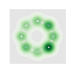
(a) Target

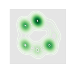
(b) GAN

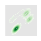
(c) MMD

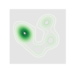
(d) EBM-10

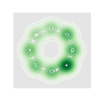
(e) Ours

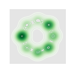
(f) GAN-m

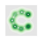
(g) MMD-m

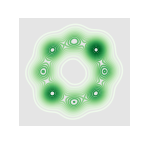
(h) EBM-30

Figure 2: Results of toy experiments. EBM-$n$ ($n=10,30$) means EBM trained with $n$-step sampling; methods appended with “-m” mean that these methods are improved with latent morphing.

We also evaluate the training time of different models, which are provided in Table 9 in the Appendix. Although EBM trained with 30-step sampling can capture all the modes, it is much more time-consuming compared to others. When the EBM is trained with a short sampling procedure, it fails to learning all the modes of the target distribution. By contrast, our proposed model and GANs are much more efficient.

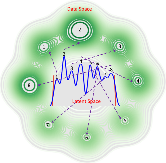
Figure 3: Latent-distribution morphing can learn an eight-mode distribution, with each mode corresponding to one mode of the target distribution.

Table 2: Comparisons of our model with related baselines.

CIFAR-10 ($32\times 32$) STL-10 ($48\times 48$) Morphing/Sampling Generator FID $(\downarrow)$ IS $(\uparrow)$ FID $(\downarrow)$ IS $(\uparrow)$ CNN-based WGAN-GP (Gulrajani et al., 2017) ✓ $28.42\pm 0.06$ $7.14\pm 0.09$ $39.88\pm 0.06$ $8.85\pm 0.09$ SN-GAN (Miyato et al., 2018) ✓ $22.30\pm 0.12$ $7.54\pm 0.09$ $40.45\pm 0.17$ $8.45\pm 0.08$ SN-SMMD-GAN (Arbel et al., 2018) ✓ $25.0\pm 0.3$ $7.3\pm 0.1$ $40.6\pm 0.1$ $8.5\pm 0.1$ CR-GAN (Zhang et al., 2019) ✓ $18.72$ $7.93$ – – Improved MMD-GAN (Wang et al., 2018) ✓ $16.21$ $8.29$ $36.67$ $9.36$ DOT (Tanaka, 2019) ✓ ✓ $15.78$ $8.50\pm 0.01$ $34.84$ $10.30\pm 0.21$ DG$f$low (Ansari et al., 2020) ✓ ✓ $15.30\pm 0.08$ $8.14\pm 0.03$ $34.60\pm 0.11$ $10.41\pm 0.02$ Ours (trained w/o morphing) ✓ ✓ $9.71\pm 0.05$ $9.24\pm 0.10$ $22.15\pm 0.12$ $11.12\pm 0.10$ Ours ✓ ✓ $\mathbf{9.01\pm 0.07}$ $\mathbf{9.38\pm 0.13}$ $\mathbf{21.40\pm 0.05}$ $\mathbf{11.17\pm 0.09}$ ResNet-based EBM (Du & Mordatch, 2019) ✓ $40.58$ $6.02$ - - NCSN (Song & Ermon, 2019) ✓ $25.32$ $8.87\pm 0.12$ - - SN-GAN (Miyato et al., 2018) ✓ $21.70\pm 0.21$ $8.22\pm 0.05$ $40.10\pm 0.50$ $9.10\pm 0.04$ CR-GAN (Zhang et al., 2019) ✓ $14.56$ $8.40$ – – BigGAN (Brock et al., 2018) ✓ $14.73$ $9.22$ – – Auto-GAN (Gong et al., 2019) ✓ $12.42$ $8.56\pm 0.10$ $31.01$ $9.16\pm 0.12$ AdversarialNAS-GAN (Gao et al., 2020) ✓ $10.87$ $8.74\pm 0.07$ $26.98$ $9.63\pm 0.19$ DOT (Tanaka, 2019) ✓ ✓ $19.71$ $8.50\pm 0.12$ $39.48$ $10.03\pm 0.14$ DDLS (Che et al., 2020) ✓ ✓ $15.42$ $9.09\pm 0.10$ - - DG$f$low (Ansari et al., 2020) ✓ ✓ $9.62\pm 0.03$ $\mathbf{9.35\pm 0.03}$ - - Ours ✓ ✓ $\mathbf{7.95\pm 0.02}$ $9.24\pm 0.11$ $\mathbf{21.23\pm 0.05}$ $\mathbf{11.17\pm 0.12}$ StyleGAN2-based StyleGAN2 (Karras et al., 2020b) ✓ $8.32\pm 0.09$ $9.21\pm 0.09$ - - StyleGAN2+ADA (Karras et al., 2020a) ✓ $2.92\pm 0.05$ $9.83\pm 0.04$ - - Ours ✓ ✓ $\mathbf{2.82\pm 0.04}$ $\mathbf{10.07\pm 0.09}$ - -

4.2 Image Generation

Main results

Following previous works (Miyato et al., 2018; Karras et al., 2020b), we conduct image generation experiments on three model achitectures: CNN-based, ResNet-based, and StyleGAN2-based models. The CNN-based model and ResNet-based model follow the architecture design as (Miyato et al., 2018), while the StyleGAN2-based model follows (Karras et al., 2020b). For fair comparisons, we use the KL divergence as the functional for optimization in (14), as other functionals will need an extra network as the variational function. Meanwhile, the functional used in (10) can be freely chosen from Table 1. Fréchet inception distance (FID) and Inception Score (IS) are reported following previous works. We compare our method with popular baselines, some of the baselines such as DG$f$low, StyleGAN2+ADA represent the state-of-the-arts in their settings.

The quantitative results are reported in Table 2. Results of the CNN-based model are from two settings: training without latent-distribution morphing and with a 5-step morphing. The ResNet-based model is trained without morphing, and the StyleGAN2-based model is based on the pre-trained model by (Karras et al., 2020a). Our proposed method obtains the best results under different architectures, which outperforms the CNN-based generative model by a large margin, and is also better than other ResNet-based generative models including the ones with Neural Architecture Search (Auto-GAN and AdversarialNAS-GAN).

Table 3: Plug-and-play on GAN-based models.

CIFAR-10 ($32\times 32$) STL-10 ($48\times 48$) Models FID $(\downarrow)$ IS $(\uparrow)$ FID $(\downarrow)$ IS $(\uparrow)$ SN-MMD-GAN $28.49\pm 0.17$ $7.18\pm 0.10$ $49.59\pm 0.06$ $7.92\pm 0.07$    + morphing $23.91\pm 0.10$ $8.26\pm 0.06$ $42.05\pm 0.11$ $9.19\pm 0.08$    + regularizer $14.60\pm 0.05$ $\mathbf{8.61\pm 0.11}$ $38.89\pm 0.06$ $9.22\pm 0.04$ SN-GAN $22.30\pm 0.12$ $7.54\pm 0.09$ $40.45\pm 0.17$ $8.45\pm 0.08$    + morphing $14.91\pm 0.09$ $8.28\pm 0.11$ $34.10\pm 0.12$ $9.13\pm 0.10$    + regularizer $\mathbf{14.45\pm 0.04}$ $8.38\pm 0.06$ $\mathbf{33.79\pm 0.05}$ $9.25\pm 0.07$ WGAN-GP $28.42\pm 0.06$ $7.14\pm 0.09$ $39.88\pm 0.06$ $8.85\pm 0.09$    + morphing $21.78\pm 0.13$ $7.89\pm 0.08$ $35.57\pm 0.05$ $9.33\pm 0.09$    + regularizer $19.15\pm 0.07$ $8.09\pm 0.11$ $34.24\pm 0.12$ $\mathbf{9.38\pm 0.05}$ SN-Sinkhorn-GAN $26.36\pm 0.15$ $7.08\pm 0.08$ $53.27\pm 0.14$ $7.58\pm 0.07$    + morphing $23.08\pm 0.07$ $7.77\pm 0.09$ $49.40\pm 0.12$ $8.14\pm 0.08$    + regularizer $21.15\pm 0.09$ $7.83\pm 0.11$ $45.44\pm 0.11$ $8.32\pm 0.10$

Plug-and-play on pre-trained GANs

We show how to improve pre-trained GANs with our latent-distribution morphing scheme for plug-and-play during testing. All the models are constructed using a 4-layer CNN generator and a 7-layer CNN discriminator as in (Miyato et al., 2018). The discriminator output dimensions of SN-MMD-GAN and SN-Sinkhorn-GAN (Genevay et al., 2018) are set to 16, while the dimensions are set to 1 for others. Quantitative results are provided in Table 3. Our proposed method indeed improves the performance, which is better than related works (Tanaka, 2019; Che et al., 2020; Ansari et al., 2020). Our plug-and-play scheme can also improve the current state-of-the-arts model trained on high-resolution images. For example, although StyleGAN2+ADA (Karras et al., 2020a) is able to generate high-resolution images with impressive details, there also exist many failure cases as shown in Figure 4. With our latent-distribution morphing scheme, many of these failure cases can be recovered, as shown in Figure 4. More results are provided in the Appendix. Specifically, the morphing process gradually refines the details while preserving some global information such as the position, foreground and background colors, etc. Some quantitative results are also provided in Table 10.

Table 4: Extension to EBMs.

CIFAR-10 ($32\times 32$) Models FID $(\downarrow)$ IS $(\uparrow)$ without generator EBM (Du & Mordatch, 2019) $37.90$ $8.30$ $f$-EBM (Yu et al., 2020) $30.86$ $8.61\pm 0.06$ Ours (EBM) $35.50\pm 0.03$ $8.60\pm 0.09$ Ours ($f$-EBM) $\mathbf{28.84\pm 0.04}$ $\mathbf{8.82\pm 0.07}$ with generator MEG (Kumar et al., 2019) $33.18$ $7.31\pm 0.06$ VERA (Grathowhl et al., 2020) $27.5$ $8.00$ GEBM (Arbel et al., 2020) $19.32$ – Ours $\mathbf{7.95\pm 0.02}$ $\mathbf{9.24\pm 0.11}$

Kernel-based EBMs

As described previously, we can construct a kernel-based variant of vanilla EBM (Du & Mordatch, 2019) or $f$-EBM (Yu et al., 2020) by removing the generator. We adopt the network architecture in (Du & Mordatch, 2019) for fairness. We can either train an EBM from scratch or directly improve the pre-trained EBM with our morphing scheme. The comparisons are provided in Table 4, we also compare our model with other methods which combine EBMs with generators. As expected, our kernel-based EBM obtains better results than the standard EBM and $f$-EBM.

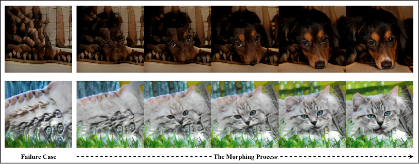
Figure 4: Failure cases mitigation with our latent-distribution morphing on the state-of-the-art StyleGAN2+ADA. First column: failure case on AFHQ Dog ($512\times 512$) and AFHQ Cat ($512\times 512$), respectively.

Table 5: FID results of the proposed method on CIFAR-10.

Steps Functional Langevin KL RKL JS SH Trained without morphing 0 $16.78\pm 0.08$ 10 $11.72\pm 0.07$ $10.45\pm 0.06$ $12.37\pm 0.08$ $11.09\pm 0.04$ $11.08\pm 0.08$ 20 $11.84\pm 0.10$ $10.12\pm 0.10$ $11.16\pm 0.10$ $10.44\pm 0.11$ $10.37\pm 0.07$ 30 $11.69\pm 0.15$ $9.81\pm 0.04$ $10.75\pm 0.06$ $9.89\pm 0.03$ $9.95\pm 0.06$ 40 $11.56\pm 0.14$ $9.88\pm 0.09$ $10.51\pm 0.07$ $9.84\pm 0.05$ $\mathbf{9.71\pm 0.05}$ Trained with 5-step morphing 0 $16.85\pm 0.05$ 10 $11.30\pm 0.08$ $9.60\pm 0.05$ $10.89\pm 0.06$ $10.45\pm 0.04$ $10.00\pm 0.04$ 20 $11.26\pm 0.03$ $9.18\pm 0.03$ $9.92\pm 0.03$ $9.56\pm 0.06$ $9.54\pm 0.04$ 30 $11.15\pm 0.06$ $9.06\pm 0.11$ $9.71\pm 0.10$ $9.28\pm 0.07$ $9.49\pm 0.05$ 40 $11.50\pm 0.05$ $\mathbf{9.01\pm 0.07}$ $9.63\pm 0.03$ $9.27\pm 0.05$ $9.32\pm 0.04$

Ablation studies

We conduct ablation studies to investigate the following questions: How do different $f$-divergence forms in latent-distribution morphing impact the model performance, and how does the number of updates in morphing during testing influence the model performance? The main results are provided in Table 5 (also Table 11 in the Appendix). From 5, we can conclude that latent-distribution morphing during training can indeed improve the model performance. However, the morphing could cost a little time overhead. Fortunately, we see from Table 5 that only performing latent-distribution morphing in testing can also improve the performance by a large margin. Empirically, we find that morphing according to the KL divergence seems to be less sensitive to hyper-parameters, which is our recommendation for practical use.

4.3 Image Translation

We apply our model for image translation based on the StarGAN v2 model (Choi et al., 2020). StarGAN v2 is able to perform high-resolution image translation over multiple domains, which consists of a generator, a mapping network, a style encoder, and a discriminator. The generator consists of an encoder and a decoder. To translate an image from a source domain to a target domain, the encoder takes the source image as input and outputs a latent feature $\operatorname{\mathbf{z}}$. Then $\operatorname{\mathbf{z}}$ and a style code $\operatorname{\mathbf{s}}$ are fed into the decoder to generate a translated image. Specifically, the style code $\operatorname{\mathbf{s}}$ is extracted by two means, corresponding to the so-called latent-guided synthesis and reference-guided synthesis.

We apply the latent-distribution morphing to StarGAN v2 to update both the style code $\operatorname{\mathbf{s}}$ and latent code $\operatorname{\mathbf{z}}$. Following (Choi et al., 2020), we conduct image translation experiment on CelebA-HQ and AFHQ by evaluating the Fréchet inception distance (FID) and learned perceptual image patch similarity (LPIPS). All images are resized to $256\times 256$. The main results are provided in Table 6 and Table 7, in which MUNIT (Huang et al., 2018), DRIT (Lee et al., 2018), MSGAN (Mao et al., 2019), StarGAN v2 serve as the baseline models. Again, our method achieves the best results. More results are provided in the Appendix.

Table 6: Results of latent-guided synthesis.

CelebA-HQ ($256\times 256$) AFHQ ($256\times 256$) Models FID $(\downarrow)$ LPIPS $(\uparrow)$ FID $(\downarrow)$ LPIPS $(\uparrow)$ MUNIT $31.4$ $0.363$ $41.5$ $0.511$ DRIT $52.1$ $0.178$ $95.6$ $0.326$ MSGAN $33.1$ $0.389$ $61.4$ $0.517$ StarGAN v2 $13.7$ $0.452$ $16.2$ $0.450$ Ours $\mathbf{13.3}$ $\mathbf{0.480}$ $\mathbf{15.8}$ 0.472

Table 7: Results of reference-guided synthesis.

CelebA-HQ ($256\times 256$) AFHQ ($256\times 256$) Models FID $(\downarrow)$ LPIPS $(\uparrow)$ FID $(\downarrow)$ LPIPS $(\uparrow)$ MUNIT $107.1$ $0.176$ $223.9$ $0.199$ DRIT $53.3$ $0.311$ $114.8$ $0.156$ MSGAN $39.6$ $0.312$ $69.8$ $0.375$ StarGAN v2 $23.8$ $0.388$ $19.8$ $0.432$ Ours $\mathbf{17.9}$ $\mathbf{0.488}$ $\mathbf{19.2}$ $\mathbf{0.457}$

5 Conclusion

We propose a new framework to learn high-dimensional distributions via a parameterized latent FP kernel. Our model not only achieves better performance than related models, but also improves arbitrary GAN and EBM by a plug-and-play mechanism. Extensive experiments have shown the effectiveness of our proposed method on various tasks.

Appendix A Proof of Lemma 1

Assume that $(q^{t})_{t\geq 0}$ evolves according to the WGF of $f$-divergence, $F(q^{t},p)=D_{f}(p\|q^{t})$, with initialization $q^{0}$. Let $d_{W_{2}}(\cdot,\cdot)$ be the 2-Wasserstein distance. Assume that $F(q^{0},p)<\infty$ and $d_{W_{2}}(q^{0},p)<\infty$. Then, the following holds:
1) $F(q^{t},p)$ is non-increasing and converges to the global optimum as $t\rightarrow\infty$;
2) If $\|\nabla_{W_{2}}F(q^{t},p)\|^{2}\geq\lambda F(q^{t},p)$ with some constant $\lambda>0$, then $F(q^{t},p)\leq\exp(-\lambda t)F(q^{0},p)$;
3) If $F(q^{t},p)$ is $\lambda$-geodesically convex with some constant $\lambda>0$, then $d_{W_{2}}(q^{t},p)\leq\exp(-\lambda t)d_{W_{2}}(q^{0},p)$;
4) If mapping $g$ is Lipschitz continuous, then $d_{W_{2}}(Q^{t},P)$ converges with the same convergence rate as $d_{W_{2}}(q^{t},p)$.

Proof 
1)

$$\dfrac{\partial F(q^{t},p)}{\partial t}=\langle\nabla_{W_{2}}F(q^{t},p),\dfrac{\partial q^{t}}{\partial t}\rangle.$$

According to the definition of Wasserstein gradient flow, we have $\dfrac{\partial q^{t}}{\partial t}=-\nabla_{W_{2}}F(q^{t},p)$. Thus, we get

$$\dfrac{\partial F(q^{t},p)}{\partial t}=-\|\nabla_{W_{2}}F(q^{t},p)\|^{2}\leq 0,$$

which means that $F(q^{t},p)$ is non-increasing. Since $F(q^{t},p)$ is $f$-divergence, we know that it will converge to a global optimum due to the convexity property, in which case $q^{\infty}=q^{*}=p,F(q^{*})=0$.

2)
For simplicity, we let $F(q^{t},p)=\mathcal{F}(t)$. Define $v(t)=\exp(\int_{0}^{t}-\lambda s\text{d}s)=\exp(-\lambda t)$. Then, we have

$$v^{\prime}(t)=\exp(-\lambda t)\cdot(-\lambda t)^{\prime}=-\lambda v(t).$$

We also know that $v(t)>0$. Thus, $v^{\prime}(t)<0$ for all $t$. Hence, we have

$$\dfrac{\text{d}}{\text{d}t}\dfrac{\mathcal{F}(t)}{v(t)} =\dfrac{\mathcal{F}^{\prime}(t)v(t)-v^{\prime}(t)\mathcal{F}(t)}{(v(t))^{2}}$$

$$=\dfrac{\mathcal{F}^{\prime}(t)v(t)+\lambda v(t)\mathcal{F}(t)}{(v(t))^{2}}$$

$$\leq\dfrac{-\lambda\mathcal{F}(t)v(t)+\lambda v(t)\mathcal{F}(t)}{(v(t))^{2}}$$

$$=0,$$

which means that $\dfrac{\mathcal{F}(t)}{v(t)}$ is non-increasing and bounded by $\dfrac{\mathcal{F}(0)}{v(0)}=\mathcal{F}(0)$. Thus, we have

$$F(q^{t},p)=\mathcal{F}(t)\leq v(t)\mathcal{F}(0)=\exp(-\lambda t)F(q^{0},p).$$

3)

Definition 5 ($\lambda$-geodesically convex)

Let $d(\cdot,\cdot)$ be the distance. A functional $\mathcal{F}$ is $\lambda$-geodesically convex if for any $v_{0},v_{1}\in\text{Domain}(\mathcal{F})$, there exists a geodesics $\gamma$ with $\gamma_{0}=v_{0},\gamma_{1}=v_{1},d(\gamma_{s},\gamma_{t})=d(\gamma_{0},\gamma_{1})(t-s),\forall 0\leq t\leq s\leq 1$ such that

$$\mathcal{F}(\gamma_{t})\leq(1-t)\mathcal{F}(\gamma_{0})+t\mathcal{(}F)(\gamma_{1})-\dfrac{1}{2}\lambda t(1-t)d^{2}(\gamma_{0},\gamma_{1}).$$

If $F(q^{t},p)$ is a $\lambda$-geodesically convex functional, we can directly apply Theorem 11.1.4 in (Ambrosio et al., 2008), by setting one of the probability measure in Theorem 11.1.4 to be the measure associated with $p$, i.e. global optimum.

4)
We have

$$d_{W_{2}}(P,Q)\leq\sqrt{\int\|\operatorname{\mathbf{x}}-\operatorname{\mathbf{x}}^{\prime}\|^{2}\text{d}\Pi}=\sqrt{\int\|g(\operatorname{\mathbf{z}})-g(\operatorname{\mathbf{z}}^{\prime})\|^{2}\text{d}\pi}\leq\sqrt{\int L^{2}\|\operatorname{\mathbf{z}}-\operatorname{\mathbf{z}}^{\prime}\|^{2}\text{d}\pi}=Ld_{W_{2}}(p,q),$$

where $\pi$ denotes the optimal transportation plan on $\mathcal{Z}^{2}$ with marginal $p,q$, $\Pi$ denotes the corresponding plan in $\mathcal{X}^{2}$, $L$ is a constant. $\Pi$ may not be the optimal plan in $\mathcal{X}^{2}$, thus we have the first inequality. By the Lipchistz continuity, we have the second inequality. The last equality comes from the definition of Wasserstein distance. Now we can easily conclude the convergence rate.  

Appendix B Details on Table 1

We would like to introduce some examples on the first variation of some functionals (Santambrogio, 2016), which will be used to help us get Table 1.

Assume that $f:R\rightarrow R$, $V:\Omega\rightarrow R$ and $W:R^{d}\rightarrow R$ are regular enough, while $W$ is symmetric. Then, the first variation of the following functionals:

$$\mathcal{F}(\rho)=\int(f(\rho)))\text{d}\operatorname{\mathbf{x}},\mathcal{V}(\rho)=\int V(\operatorname{\mathbf{x}})\text{d}\rho,\mathcal{W}(\rho)=\dfrac{1}{2}\int\int W(\operatorname{\mathbf{x}}-\operatorname{\mathbf{y}})\text{d}\rho(\operatorname{\mathbf{x}})\text{d}\rho(\operatorname{\mathbf{y}})$$

are

$$\dfrac{\delta\mathcal{F}}{\delta\rho}(\rho)=f^{\prime}(\rho),\dfrac{\delta\mathcal{V}}{\delta\rho}(\rho)=V,\dfrac{\delta\mathcal{W}}{\delta\rho}(\rho)=W*\rho.$$

Recall that in the morphing, we are trying to match the latent distribution $r(\operatorname{\mathbf{z}})$ with target parametric distribution $q(\operatorname{\mathbf{z}})$ (not $p(\operatorname{\mathbf{z}})$), and we approximate $r(\operatorname{\mathbf{z}})$ by $\sum_{i=1}^{n}K(g(\operatorname{\mathbf{z}}),g(\operatorname{\mathbf{z}}_{i}))$, and $q(\operatorname{\mathbf{z}})\propto\int K(g(\operatorname{\mathbf{z}}),\operatorname{\mathbf{x}}^{\prime})P(\operatorname{\mathbf{x}}^{\prime})\text{d}(\operatorname{\mathbf{x}}^{\prime})\approx\sum_{i=1}^{n}K(g(\operatorname{\mathbf{z}}),\operatorname{\mathbf{x}}^{\prime}_{i})/n$.

1) In the case of KL-divergence, $F(r)=\int r\log(r/q)\text{d}\operatorname{\mathbf{x}}$. We have

$$\dfrac{\delta F(r)}{\delta r}=\log(r/q).$$

Thus,

$$\nabla_{\operatorname{\mathbf{z}}}\dfrac{\delta F(r)}{\delta r}=\nabla_{\operatorname{\mathbf{z}}}\log\sum_{i=1}^{n}K(g(\operatorname{\mathbf{z}}),g(\operatorname{\mathbf{z}}_{i}))-\nabla_{\operatorname{\mathbf{z}}}\log\sum_{i=1}^{n}K(g(\operatorname{\mathbf{z}}),\operatorname{\mathbf{x}}^{\prime}_{i}).$$

2) In the case of reverse KL-divergence, $F(r)=\int q\log(q/r)\text{d}\operatorname{\mathbf{x}}$. We have

$$\dfrac{\delta F(r)}{\delta r}=-\dfrac{q}{r}.$$

Thus,

$$\nabla_{\operatorname{\mathbf{z}}}\dfrac{\delta F(r)}{\delta r}\propto-\nabla_{\operatorname{\mathbf{z}}}\left[\sum_{i}^{n}K(g(\operatorname{\mathbf{z}}),\operatorname{\mathbf{x}}^{\prime}_{i})/\sum_{i}^{n}K(g(\operatorname{\mathbf{z}}),g(\operatorname{\mathbf{z}}_{i}))\right].$$

We use ”$\propto$” instead of ”$=$” due to the existence of normalization constant of $q(\operatorname{\mathbf{z}})$ and $r(\operatorname{\mathbf{z}})$. This will not influence our method because we will choose a hyper-parameter: step size $\lambda$, which will scale the gradient and cancel the impact of the unknown constant.

3) In the case of JS-divergence, $F(r)=\dfrac{1}{2}\int r\log\dfrac{2r}{r+q}+q\log\dfrac{2q}{r+q}\text{d}\operatorname{\mathbf{x}}$. We have

$$\dfrac{\delta F(r)}{\delta r}=\dfrac{1}{2}\log\dfrac{2r}{r+q}-\dfrac{1}{4}.$$

Thus,

$$\nabla_{\operatorname{\mathbf{z}}}\dfrac{\delta F(r)}{\delta r}=-\dfrac{1}{2}\Big{\{}\nabla_{\operatorname{\mathbf{x}}}\log\left[\sum_{i}^{n}K(g(\operatorname{\mathbf{z}}),g(\operatorname{\mathbf{z}}_{i}))+\sum_{i}^{n}\alpha K(g(\operatorname{\mathbf{z}}),\operatorname{\mathbf{x}}^{\prime}_{i})\right]-\nabla_{\operatorname{\mathbf{z}}}\log 2\sum_{i}^{n}K(g(\operatorname{\mathbf{z}}),g(\operatorname{\mathbf{z}}_{i}))\Big{\}}.$$

where $\alpha$ is a hyper-parameter because of the existence of normalization constant of $q(\operatorname{\mathbf{z}})$ and $r(\operatorname{\mathbf{z}})$. In practice, $\alpha=1$ works well. Thus, we simply set $\alpha=1$ in experiments.

4) In the case of SH-divergence, $F(r)=\int(\sqrt{r}-\sqrt{q})^{2}\text{d}\operatorname{\mathbf{x}}$. We have

$$\dfrac{\delta F(r)}{\delta r}=1-\sqrt{\dfrac{q}{r}}.$$

Thus,

$$\nabla_{\operatorname{\mathbf{z}}}\dfrac{\delta F(r)}{\delta r}\propto-\nabla_{\operatorname{\mathbf{z}}}\sqrt{\sum_{i}^{n}K(g(\operatorname{\mathbf{z}}),\operatorname{\mathbf{x}}^{\prime}_{i})/\sum_{i}^{n}K(g(\operatorname{\mathbf{z}}),g(\operatorname{\mathbf{z}}_{i}))}.$$

The normalization constants of $q(\operatorname{\mathbf{z}})$ and $r(\operatorname{\mathbf{z}})$ are hidden in the proportion.

Appendix C Discussion on Training Generator

As mentioned earlier, we train the generator $g_{{\bm{\theta}}}$ by minimizing $\text{MMD}_{\boldsymbol{\phi}}(P,R)$ because we do not have closed form of $R(\operatorname{\mathbf{x}})$. The gradient of MMD w.r.t ${\bm{\theta}}$ is

$$\nabla_{{\bm{\theta}}}\text{MMD}_{\boldsymbol{\phi}}(P,R)= \nabla_{{\bm{\theta}}}\{\mathbb{E}_{R(\operatorname{\mathbf{x}}),R(\operatorname{\mathbf{x}}^{\prime})}\left[K_{\boldsymbol{\phi}}(\operatorname{\mathbf{x}},\operatorname{\mathbf{x}}^{\prime})\right]-2\mathbb{E}_{R(\operatorname{\mathbf{x}}),P(\operatorname{\mathbf{x}}^{\prime})}\left[K_{\boldsymbol{\phi}}(\operatorname{\mathbf{x}},\operatorname{\mathbf{x}}^{\prime})\right]+\mathbb{E}_{P(\operatorname{\mathbf{x}}),P(\operatorname{\mathbf{x}}^{\prime})}\left[K_{\boldsymbol{\phi}}(\operatorname{\mathbf{x}},\operatorname{\mathbf{x}}^{\prime})\right]\}$$

$$= \nabla_{{\bm{\theta}}}\{\mathbb{E}_{r(\operatorname{\mathbf{z}}),r(\operatorname{\mathbf{z}}^{\prime})}\left[K_{\boldsymbol{\phi}}(g_{{\bm{\theta}}}(\operatorname{\mathbf{z}}),g_{{\bm{\theta}}}(\operatorname{\mathbf{z}}^{\prime}))\right]-2\mathbb{E}_{r(\operatorname{\mathbf{z}}),P(\operatorname{\mathbf{x}}^{\prime})}\left[K_{\boldsymbol{\phi}}(g_{{\bm{\theta}}}(\operatorname{\mathbf{z}}),\operatorname{\mathbf{x}}^{\prime})\right]+\mathbb{E}_{P(\operatorname{\mathbf{x}}),P(\operatorname{\mathbf{x}}^{\prime})}\left[K_{\boldsymbol{\phi}}(\operatorname{\mathbf{x}},\operatorname{\mathbf{x}}^{\prime})\right]\}$$

$$= \mathbb{E}_{r(\operatorname{\mathbf{z}}),r(\operatorname{\mathbf{z}}^{\prime})}\left[\nabla_{{\bm{\theta}}}K_{\boldsymbol{\phi}}(g_{{\bm{\theta}}}(\operatorname{\mathbf{z}}),g_{{\bm{\theta}}}(\operatorname{\mathbf{z}}^{\prime}))\right]-2\mathbb{E}_{r(\operatorname{\mathbf{z}}),P(\operatorname{\mathbf{x}}^{\prime})}\left[\nabla_{{\bm{\theta}}}K_{\boldsymbol{\phi}}(g_{{\bm{\theta}}}(\operatorname{\mathbf{z}}),\operatorname{\mathbf{x}}^{\prime})\right].$$

We assume that $R(\operatorname{\mathbf{x}})=R(g_{{\bm{\theta}}}(\operatorname{\mathbf{z}}))\propto r(\operatorname{\mathbf{z}})=\mathbb{E}_{r(\operatorname{\mathbf{z}}^{\prime})}\left[K_{\boldsymbol{\phi}}(g_{{\bm{\theta}}}(\operatorname{\mathbf{z}}),g_{{\bm{\theta}}}(\operatorname{\mathbf{z}}^{\prime}))\right]$. We rewrite this as

$$R(g_{{\bm{\theta}}}(\operatorname{\mathbf{z}}))=\dfrac{\mathbb{E}_{r(\operatorname{\mathbf{z}}^{\prime})}\left[K_{\boldsymbol{\phi}}(g_{{\bm{\theta}}}(\operatorname{\mathbf{z}}),g_{{\bm{\theta}}}(\operatorname{\mathbf{z}}^{\prime}))\right]}{C},$$

where $C=\int\mathbb{E}_{r(\operatorname{\mathbf{z}}^{\prime})}\left[K_{\boldsymbol{\phi}}(g_{{\bm{\theta}}}(\operatorname{\mathbf{z}}),g_{{\bm{\theta}}}(\operatorname{\mathbf{z}}^{\prime}))\right]\text{d}\operatorname{\mathbf{z}}$ is the normalization constant. The gradient of negative log-likelihood w.r.t ${\bm{\theta}}$ is

$$-\nabla_{{\bm{\theta}}}\mathbb{E}_{P(\operatorname{\mathbf{x}})}\left[\log R(\operatorname{\mathbf{x}})\right]$$

$$= -\nabla_{{\bm{\theta}}}\mathbb{E}_{p(\operatorname{\mathbf{z}})}\left[\log R(g_{{\bm{\theta}}}(\operatorname{\mathbf{z}})\right]$$

$$= -\mathbb{E}_{p(\operatorname{\mathbf{z}})}\{\nabla_{{\bm{\theta}}}\log\mathbb{E}_{r(\operatorname{\mathbf{z}}^{\prime})}\left[K_{\boldsymbol{\phi}}(g_{{\bm{\theta}}}(\operatorname{\mathbf{z}}),g_{{\bm{\theta}}}(\operatorname{\mathbf{z}}^{\prime}))\right]-\nabla_{{\bm{\theta}}}\log C\}$$

$$= -\mathbb{E}_{P(\operatorname{\mathbf{x}})}\{\nabla_{{\bm{\theta}}}\log\mathbb{E}_{r(\operatorname{\mathbf{z}}^{\prime})}\left[K_{\boldsymbol{\phi}}(\operatorname{\mathbf{x}},g_{{\bm{\theta}}}(\operatorname{\mathbf{z}}^{\prime}))\right]\}+\mathbb{E}_{P(\operatorname{\mathbf{x}})}\left[\nabla_{{\bm{\theta}}}\log C\right]$$

$$= -\mathbb{E}_{P(\operatorname{\mathbf{x}})}\Big{\{}\dfrac{\nabla_{{\bm{\theta}}}\mathbb{E}_{r(\operatorname{\mathbf{z}}^{\prime})}\left[K_{\boldsymbol{\phi}}(g_{{\bm{\theta}}}(\operatorname{\mathbf{z}}^{\prime}),\operatorname{\mathbf{x}})\right]}{\mathbb{E}_{r(\operatorname{\mathbf{z}}^{\prime})}\left[K_{\boldsymbol{\phi}}(\operatorname{\mathbf{x}},g_{{\bm{\theta}}}(\operatorname{\mathbf{z}}^{\prime}))\right]}\Big{\}}+\mathbb{E}_{P(\operatorname{\mathbf{x}})}\left[\dfrac{\nabla_{{\bm{\theta}}}C}{C}\right]$$

$$= -\mathbb{E}_{P(\operatorname{\mathbf{x}})}\Big{\{}\dfrac{\mathbb{E}_{r(\operatorname{\mathbf{z}}^{\prime})}\left[\nabla_{{\bm{\theta}}}K_{\boldsymbol{\phi}}(g_{{\bm{\theta}}}(\operatorname{\mathbf{z}}^{\prime}),\operatorname{\mathbf{x}})\right]}{\mathbb{E}_{r(\operatorname{\mathbf{z}}^{\prime})}\left[K_{\boldsymbol{\phi}}(\operatorname{\mathbf{x}},g_{{\bm{\theta}}}(\operatorname{\mathbf{z}}^{\prime}))\right]}\Big{\}}+\mathbb{E}_{P(\operatorname{\mathbf{x}})}\left[\dfrac{\int\nabla_{{\bm{\theta}}}\int r(\operatorname{\mathbf{z}}^{\prime})K_{\boldsymbol{\phi}}(g_{{\bm{\theta}}}(\operatorname{\mathbf{z}}),g_{{\bm{\theta}}}(\operatorname{\mathbf{z}}^{\prime}))\text{d}\operatorname{\mathbf{z}}^{\prime}\text{d}\operatorname{\mathbf{z}}}{C}\right]$$

$$= -\mathbb{E}_{P(\operatorname{\mathbf{x}})}\Big{\{}\dfrac{\mathbb{E}_{r(\operatorname{\mathbf{z}}^{\prime})}\left[\nabla_{{\bm{\theta}}}K_{\boldsymbol{\phi}}(g_{{\bm{\theta}}}(\operatorname{\mathbf{z}}^{\prime}),\operatorname{\mathbf{x}})\right]}{\mathbb{E}_{r(\operatorname{\mathbf{z}}^{\prime})}\left[K_{\boldsymbol{\phi}}(g_{{\bm{\theta}}}(\operatorname{\mathbf{z}}^{\prime}),\operatorname{\mathbf{x}})\right]}\Big{\}}+\mathbb{E}_{P(\operatorname{\mathbf{x}})}\left[\dfrac{\int\int r(\operatorname{\mathbf{z}}^{\prime})K_{\boldsymbol{\phi}}(g_{{\bm{\theta}}}(\operatorname{\mathbf{z}}),g_{{\bm{\theta}}}(\operatorname{\mathbf{z}}^{\prime}))\text{d}\operatorname{\mathbf{z}}^{\prime}\nabla_{{\bm{\theta}}}\log(\int r(\operatorname{\mathbf{z}}^{\prime})K_{\boldsymbol{\phi}}(g_{{\bm{\theta}}}(\operatorname{\mathbf{z}}),g_{{\bm{\theta}}}(\operatorname{\mathbf{z}}^{\prime}))\text{d}\operatorname{\mathbf{z}}^{\prime}\text{d}\operatorname{\mathbf{z}})}{C}\right]$$

$$= -\mathbb{E}_{P(\operatorname{\mathbf{x}})}\Big{\{}\dfrac{\mathbb{E}_{r(\operatorname{\mathbf{z}}^{\prime})}\left[\nabla_{{\bm{\theta}}}K_{\boldsymbol{\phi}}(g_{{\bm{\theta}}}(\operatorname{\mathbf{z}}^{\prime}),\operatorname{\mathbf{x}})\right]}{\mathbb{E}_{r(\operatorname{\mathbf{z}}^{\prime})}\left[K_{\boldsymbol{\phi}}(g_{{\bm{\theta}}}(\operatorname{\mathbf{z}}^{\prime}),\operatorname{\mathbf{x}})\right]}\Big{\}}+\int R(g_{{\bm{\theta}}}(\operatorname{\mathbf{z}}))\nabla_{{\bm{\theta}}}\log(\int r(\operatorname{\mathbf{z}}^{\prime})K_{\boldsymbol{\phi}}(g_{{\bm{\theta}}}(\operatorname{\mathbf{z}}),g_{{\bm{\theta}}}(\operatorname{\mathbf{z}}^{\prime}))\text{d}\operatorname{\mathbf{z}}^{\prime})\text{d}\operatorname{\mathbf{z}}$$

$$= -\mathbb{E}_{P(\operatorname{\mathbf{x}})}\Big{\{}\dfrac{\mathbb{E}_{r(\operatorname{\mathbf{z}}^{\prime})}\left[\nabla_{{\bm{\theta}}}K_{\boldsymbol{\phi}}(g_{{\bm{\theta}}}(\operatorname{\mathbf{z}}^{\prime}),\operatorname{\mathbf{x}})\right]}{\mathbb{E}_{r(\operatorname{\mathbf{z}}^{\prime})}\left[K_{\boldsymbol{\phi}}(g_{{\bm{\theta}}}(\operatorname{\mathbf{z}}^{\prime}),\operatorname{\mathbf{x}})\right]}\Big{\}}+\mathbb{E}_{r(\operatorname{\mathbf{z}})}\Big{\{}\dfrac{\mathbb{E}_{r(\operatorname{\mathbf{z}}^{\prime})}\left[\nabla_{{\bm{\theta}}}K_{\boldsymbol{\phi}}(g_{{\bm{\theta}}}(\operatorname{\mathbf{z}}),g_{{\bm{\theta}}}(\operatorname{\mathbf{z}}^{\prime}))\right]}{\mathbb{E}_{r(\operatorname{\mathbf{z}}^{\prime})}\left[K_{\boldsymbol{\phi}}(g_{{\bm{\theta}}}(\operatorname{\mathbf{z}}),g_{{\bm{\theta}}}(\operatorname{\mathbf{z}}^{\prime}))\right]}\Big{\}}.$$

We can see that these two gradients are very similar to each other, except that the second one has extra terms scaling the gradient. Applying gradient descent with either is equivalent to minimizing $K_{\boldsymbol{\phi}}(g_{{\bm{\theta}}}(\operatorname{\mathbf{z}}),g_{{\bm{\theta}}}(\operatorname{\mathbf{z}}^{\prime}))$ and maximizing $K_{\boldsymbol{\phi}}(g_{{\bm{\theta}}}(\operatorname{\mathbf{z}}),\operatorname{\mathbf{x}})$, where $\operatorname{\mathbf{z}},\operatorname{\mathbf{z}}^{\prime}\sim r(\operatorname{\mathbf{z}}),\operatorname{\mathbf{x}}\sim P(\operatorname{\mathbf{x}})$. Intuitively, this is training the generator to generate samples that are similar to real samples (by maximizing the similarity between generated samples and real ones), while the generated samples should be diverse enough (by minimizing the similarity between generated samples).

Appendix D Proof of Theorem 4

For distribution $q(\operatorname{\mathbf{z}})$ parameterized as (6), the gradient of arbitrary $f$-divergence $D_{f}(p\|q)=\mathbb{E}_{q(\operatorname{\mathbf{z}})}\left[f(p(\operatorname{\mathbf{z}})/q(\operatorname{\mathbf{z}}))\right]$ w.r.t. $\boldsymbol{\phi}$ can be written as:

$$\nabla_{\boldsymbol{\phi}}D_{f}(p\|q)=-\mathbb{E}_{q(\operatorname{\mathbf{z}})}\Big{\{}f^{*}(v^{*}(\operatorname{\mathbf{z}}))\nabla_{\boldsymbol{\phi}}\log\{\mathbb{E}_{P(\operatorname{\mathbf{x}}^{\prime})}\left[K_{\boldsymbol{\phi}}(g_{{\bm{\theta}}}(\operatorname{\mathbf{z}}),\operatorname{\mathbf{x}}^{\prime})\right]\}\Big{\}}+\mathbb{E}_{q(\operatorname{\mathbf{z}})}\left[f^{*}(v^{*}(\operatorname{\mathbf{z}}))\right]\mathbb{E}_{q(\operatorname{\mathbf{z}})}\big{\{}\nabla_{\boldsymbol{\phi}}\log\{\mathbb{E}_{P(\operatorname{\mathbf{x}}^{\prime})}\left[K_{\boldsymbol{\phi}}(g_{{\bm{\theta}}}(\operatorname{\mathbf{z}}),\operatorname{\mathbf{x}}^{\prime})\right]\}\big{\}}.$$

Specifically, the gradient of KL divergence $D_{KL}(p\|q)$ w.r.t. $\boldsymbol{\phi}$ can be written as:

$$\nabla_{\boldsymbol{\phi}}D_{KL}(p\|q)=-\mathbb{E}_{P(\operatorname{\mathbf{x}})}\{\nabla_{\boldsymbol{\phi}}\log\{\mathbb{E}_{P(\operatorname{\mathbf{x}}^{\prime})}\left[K_{\boldsymbol{\phi}}(\operatorname{\mathbf{x}},\operatorname{\mathbf{x}}^{\prime})\right]\}\}+\mathbb{E}_{q(\operatorname{\mathbf{z}})}\{\nabla_{\boldsymbol{\phi}}\log\{\mathbb{E}_{P(\operatorname{\mathbf{x}}^{\prime})}\left[K_{\boldsymbol{\phi}}(g_{{\bm{\theta}}}(\operatorname{\mathbf{z}}),\operatorname{\mathbf{x}}^{\prime})\right]\}\}.$$

Proof  Recall that our parameterization

$$q(\operatorname{\mathbf{z}})=\tilde{q}(\operatorname{\mathbf{x}})/Z=\int K_{\boldsymbol{\phi}}(g_{{\bm{\theta}}}(\operatorname{\mathbf{z}}),\operatorname{\mathbf{x}})P(\operatorname{\mathbf{x}}^{\prime})\text{d}\operatorname{\mathbf{x}}^{\prime}/Z_{\boldsymbol{\phi}},Z_{\boldsymbol{\phi}}=\int\int K_{\boldsymbol{\phi}}(g_{{\bm{\theta}}}(\operatorname{\mathbf{z}}),\operatorname{\mathbf{x}})P(\operatorname{\mathbf{x}}^{\prime})\text{d}\operatorname{\mathbf{x}}^{\prime}\text{d}\operatorname{\mathbf{z}}$$

and the variational representation of $f$-divergence (Nguyen et al., 2010) is:

$$D_{f}(p\|q)=\sup_{v\in\mathcal{V}}\mathbb{E}_{p(\operatorname{\mathbf{z}})}\left[v(\operatorname{\mathbf{z}})\right]-\mathbb{E}_{q(\operatorname{\mathbf{z}})}\left[f^{*}(v(\operatorname{\mathbf{z}}))\right],$$

where $f^{*}$ is the Fenchel conjugate function of $f$, and sub-differential $\partial f(p/q)$ contains an element of $\mathcal{V}$. Let $v^{*}\in\mathcal{V}$ be the function when supremum is attained, we have

$$\nabla_{\boldsymbol{\phi}}D_{f}(p\|q) =-\nabla_{\boldsymbol{\phi}}\mathbb{E}_{q(\operatorname{\mathbf{z}})}\left[f^{*}(v^{*}(\operatorname{\mathbf{z}}))\right]$$

$$=-\int\nabla_{\boldsymbol{\phi}}q(\operatorname{\mathbf{z}})f^{*}(v^{*}(\operatorname{\mathbf{z}}))\text{d}\operatorname{\mathbf{z}}$$

$$=-\int q(\operatorname{\mathbf{z}})\{\nabla_{\boldsymbol{\phi}}\log\int K_{\boldsymbol{\phi}}(g_{{\bm{\theta}}}(\operatorname{\mathbf{z}}),\operatorname{\mathbf{x}}^{\prime})P(\operatorname{\mathbf{x}}^{\prime})\text{d}\operatorname{\mathbf{x}}^{\prime}-\nabla_{\boldsymbol{\phi}}\log Z_{\boldsymbol{\phi}}\}f^{*}(v^{*}(\operatorname{\mathbf{z}}))\text{d}\operatorname{\mathbf{z}}$$

$$=-\int q(\operatorname{\mathbf{z}})f^{*}(v^{*}(\operatorname{\mathbf{x}}))\nabla_{\boldsymbol{\phi}}\log\int K_{\boldsymbol{\phi}}(g_{{\bm{\theta}}}(\operatorname{\mathbf{z}}),\operatorname{\mathbf{x}}^{\prime})P(\operatorname{\mathbf{x}}^{\prime})\text{d}\operatorname{\mathbf{x}}^{\prime}\text{d}\operatorname{\mathbf{z}}+\int q(\operatorname{\mathbf{z}})f^{*}(v^{*}(\operatorname{\mathbf{x}}))\nabla_{\boldsymbol{\phi}}\log Z_{\boldsymbol{\phi}}\text{d}\operatorname{\mathbf{z}}$$

$$=-\mathbb{E}_{q(\operatorname{\mathbf{z}})}\{f^{*}(v^{*}(\operatorname{\mathbf{z}}))\nabla_{\boldsymbol{\phi}}\log\{\mathbb{E}_{P(\operatorname{\mathbf{x}}^{\prime})}\left[K_{\boldsymbol{\phi}}(g_{{\bm{\theta}}}(\operatorname{\mathbf{z}}),\operatorname{\mathbf{x}}^{\prime})\right]\}\}+\int q(\operatorname{\mathbf{z}})f^{*}(v^{*}(\operatorname{\mathbf{z}}))\dfrac{\nabla_{\boldsymbol{\phi}}Z_{\boldsymbol{\phi}}}{Z_{\boldsymbol{\phi}}}\text{d}\operatorname{\mathbf{z}}$$

$$=-\mathbb{E}_{q(\operatorname{\mathbf{z}})}\{f^{*}(v^{*}(\operatorname{\mathbf{z}}))\nabla_{\boldsymbol{\phi}}\log\{\mathbb{E}_{P(\operatorname{\mathbf{x}}^{\prime})}\left[K_{\boldsymbol{\phi}}(g_{{\bm{\theta}}}(\operatorname{\mathbf{z}}),\operatorname{\mathbf{x}}^{\prime})\right]\}\}+\int q(\operatorname{\mathbf{z}})f^{*}(v^{*}(\operatorname{\mathbf{z}}))\dfrac{\nabla_{\boldsymbol{\phi}}\int\int K_{\boldsymbol{\phi}}(g_{{\bm{\theta}}}(\operatorname{\mathbf{z}}^{\prime}),\operatorname{\mathbf{x}}^{\prime})P(\operatorname{\mathbf{x}}^{\prime})\text{d}\operatorname{\mathbf{x}}^{\prime}\text{d}\operatorname{\mathbf{z}}^{\prime}}{Z_{\boldsymbol{\phi}}}\text{d}\operatorname{\mathbf{z}}$$

$$=-\mathbb{E}_{q(\operatorname{\mathbf{z}})}\{f^{*}(v^{*}(\operatorname{\mathbf{z}}))\nabla_{\boldsymbol{\phi}}\log\{\mathbb{E}_{P(\operatorname{\mathbf{x}}^{\prime})}\left[K_{\boldsymbol{\phi}}(g_{{\bm{\theta}}}(\operatorname{\mathbf{z}}),\operatorname{\mathbf{x}}^{\prime})\right]\}\}$$

$$\quad+\int q(\operatorname{\mathbf{z}})f^{*}(v^{*}(\operatorname{\mathbf{z}}))\text{d}\operatorname{\mathbf{z}}\cdot\dfrac{\int\tilde{q}(\operatorname{\mathbf{z}})\nabla_{\boldsymbol{\phi}}\log\int K_{\boldsymbol{\phi}}(g_{{\bm{\theta}}}(\operatorname{\mathbf{z}}),\operatorname{\mathbf{x}}^{\prime})P(\operatorname{\mathbf{x}}^{\prime})\text{d}\operatorname{\mathbf{x}}^{\prime}\text{d}\operatorname{\mathbf{z}}}{Z_{\boldsymbol{\phi}}}$$

$$=-\mathbb{E}_{q(\operatorname{\mathbf{z}})}\Big{\{}f^{*}(v^{*}(\operatorname{\mathbf{z}}))\nabla_{\boldsymbol{\phi}}\log\{\mathbb{E}_{P(\operatorname{\mathbf{x}}^{\prime})}\left[K_{\boldsymbol{\phi}}(g_{{\bm{\theta}}}(\operatorname{\mathbf{z}}),\operatorname{\mathbf{x}}^{\prime})\right]\}\Big{\}}+\mathbb{E}_{q(\operatorname{\mathbf{z}})}\left[f^{*}(v^{*}(\operatorname{\mathbf{z}}))\right]\mathbb{E}_{q(\operatorname{\mathbf{z}})}\big{\{}\nabla_{\boldsymbol{\phi}}\log\{\mathbb{E}_{P(\operatorname{\mathbf{x}}^{\prime})}\left[K_{\boldsymbol{\phi}}(g_{{\bm{\theta}}}(\operatorname{\mathbf{z}}),\operatorname{\mathbf{x}}^{\prime})\right]\}\big{\}}.$$

For KL-divergence, we have:

$$\nabla_{\boldsymbol{\phi}}D_{KL}(p\|q)$$

$$= -\nabla_{\boldsymbol{\phi}}\mathbb{E}_{p(\operatorname{\mathbf{z}})}\left[\log q(\operatorname{\mathbf{z}})\right]$$

$$= -\mathbb{E}_{p(\operatorname{\mathbf{z}})}\left[\nabla_{\boldsymbol{\phi}}\log\int K_{\boldsymbol{\phi}}(g_{{\bm{\theta}}}(\operatorname{\mathbf{z}}),\operatorname{\mathbf{x}}^{\prime})P(\operatorname{\mathbf{x}}^{\prime})\text{d}\operatorname{\mathbf{x}}^{\prime}-\nabla_{\boldsymbol{\phi}}\log Z_{\boldsymbol{\phi}}\right]$$

$$= -\mathbb{E}_{p(\operatorname{\mathbf{z}})}\left[\nabla_{\boldsymbol{\phi}}\log\int K_{\boldsymbol{\phi}}(g_{{\bm{\theta}}}(\operatorname{\mathbf{z}}),\operatorname{\mathbf{x}}^{\prime})P(\operatorname{\mathbf{x}}^{\prime})\text{d}\operatorname{\mathbf{x}}^{\prime}\right]+\mathbb{E}_{p(\operatorname{\mathbf{z}})}\left[\nabla_{\boldsymbol{\phi}}\log Z_{\boldsymbol{\phi}}\right]$$

$$= -\mathbb{E}_{P(\operatorname{\mathbf{x}})}\left[\nabla_{\boldsymbol{\phi}}\log\int K_{\boldsymbol{\phi}}(\operatorname{\mathbf{x}},\operatorname{\mathbf{x}}^{\prime})P(\operatorname{\mathbf{x}}^{\prime})\text{d}\operatorname{\mathbf{x}}^{\prime}\right]+\mathbb{E}_{p(\operatorname{\mathbf{z}})}\left[\dfrac{\nabla_{\boldsymbol{\phi}}Z_{\boldsymbol{\phi}}}{Z_{\boldsymbol{\phi}}}\right]$$

$$= -\mathbb{E}_{P(\operatorname{\mathbf{x}})}\{\nabla_{\boldsymbol{\phi}}\log\{\mathbb{E}_{P(\operatorname{\mathbf{x}}^{\prime})}\left[K_{\boldsymbol{\phi}}(\operatorname{\mathbf{x}},\operatorname{\mathbf{x}}^{\prime})\right]\}\}+\mathbb{E}_{p(\operatorname{\mathbf{z}})}\left[\dfrac{\nabla_{\boldsymbol{\phi}}\int\int K_{\boldsymbol{\phi}}(g_{{\bm{\theta}}}(\operatorname{\mathbf{z}}),\operatorname{\mathbf{x}}^{\prime})P(\operatorname{\mathbf{x}}^{\prime})\text{d}\operatorname{\mathbf{x}}^{\prime}\text{d}\operatorname{\mathbf{z}}}{Z_{\boldsymbol{\phi}}}\right]$$

$$= -\mathbb{E}_{P(\operatorname{\mathbf{x}})}\{\nabla_{\boldsymbol{\phi}}\log\{\mathbb{E}_{P(\operatorname{\mathbf{x}}^{\prime})}\left[K_{\boldsymbol{\phi}}(\operatorname{\mathbf{x}},\operatorname{\mathbf{x}}^{\prime})\right]\}\}+\mathbb{E}_{p(\operatorname{\mathbf{z}})}\left[\dfrac{\int\int K_{\boldsymbol{\phi}}(g_{{\bm{\theta}}}(\operatorname{\mathbf{z}}),\operatorname{\mathbf{x}}^{\prime})P(\operatorname{\mathbf{x}}^{\prime})\text{d}\operatorname{\mathbf{x}}^{\prime}\cdot\nabla_{\boldsymbol{\phi}}\log\int K_{\boldsymbol{\phi}}(g_{{\bm{\theta}}}(\operatorname{\mathbf{z}}),\operatorname{\mathbf{x}}^{\prime})P(\operatorname{\mathbf{x}}^{\prime})\text{d}\operatorname{\mathbf{x}}^{\prime}\text{d}\operatorname{\mathbf{z}}}{Z_{\boldsymbol{\phi}}}\right]$$

$$= -\mathbb{E}_{P(\operatorname{\mathbf{x}})}\{\nabla_{\boldsymbol{\phi}}\log\{\mathbb{E}_{P(\operatorname{\mathbf{x}}^{\prime})}\left[K_{\boldsymbol{\phi}}(\operatorname{\mathbf{x}},\operatorname{\mathbf{x}}^{\prime})\right]\}\}+\mathbb{E}_{p(\operatorname{\mathbf{z}})}\left[\dfrac{\int\tilde{q}(\operatorname{\mathbf{z}})\nabla_{\boldsymbol{\phi}}\log\int K_{\boldsymbol{\phi}}(g_{{\bm{\theta}}}(\operatorname{\mathbf{z}}),\operatorname{\mathbf{x}}^{\prime})P(\operatorname{\mathbf{x}}^{\prime})\text{d}\operatorname{\mathbf{x}}^{\prime}\text{d}\operatorname{\mathbf{x}}}{Z_{\boldsymbol{\phi}}}\right]$$

$$= -\mathbb{E}_{P(\operatorname{\mathbf{x}})}\{\nabla_{\boldsymbol{\phi}}\log\{\mathbb{E}_{P(\operatorname{\mathbf{x}}^{\prime})}\left[K_{\boldsymbol{\phi}}(\operatorname{\mathbf{x}},\operatorname{\mathbf{x}}^{\prime})\right]\}\}+\mathbb{E}_{p(\operatorname{\mathbf{z}})}\{\mathbb{E}_{q(\operatorname{\mathbf{z}})}\{\nabla_{\boldsymbol{\phi}}\log\{\mathbb{E}_{P(\operatorname{\mathbf{x}}^{\prime})}\left[K_{\boldsymbol{\phi}}(g_{{\bm{\theta}}}(\operatorname{\mathbf{z}}),\operatorname{\mathbf{x}}^{\prime})\right]\}\}\}$$

$$= -\mathbb{E}_{P(\operatorname{\mathbf{x}})}\{\nabla_{\boldsymbol{\phi}}\log\{\mathbb{E}_{P(\operatorname{\mathbf{x}}^{\prime})}\left[K_{\boldsymbol{\phi}}(\operatorname{\mathbf{x}},\operatorname{\mathbf{x}}^{\prime})\right]\}\}+\mathbb{E}_{q(\operatorname{\mathbf{z}})}\{\nabla_{\boldsymbol{\phi}}\log\{\mathbb{E}_{P(\operatorname{\mathbf{x}}^{\prime})}\left[K_{\boldsymbol{\phi}}(g_{{\bm{\theta}}}(\operatorname{\mathbf{z}}),\operatorname{\mathbf{x}}^{\prime})\right]\}\}.$$

 

Appendix E Discussion on $f^{*}$ and $v^{*}$

We provide some conjugate functions $f^{*}$ of different $f$-divergence in Table 8, readers interested in using $f$-divergence in GANs and EBMs may also refer to (Nowozin et al., 2016; Yu et al., 2020).

Table 8: Examples of $f^{*}$ for different $f$-divergence

$f$-divergence $D_{f}(p\|q)$ $f(u)$ $f^{*}(t)$ Kullback-Leibler $\int p(\operatorname{\mathbf{x}})\log\dfrac{p(\operatorname{\mathbf{x}})}{q(\operatorname{\mathbf{x}})}d\operatorname{\mathbf{x}}$ $u\log u$ $\exp(t-1)$ Reverse Kullback-Leibler $\int q(\operatorname{\mathbf{x}})\log\dfrac{q(\operatorname{\mathbf{x}})}{p(\operatorname{\mathbf{x}})}d\operatorname{\mathbf{x}}$ $-\log u$ $-1-\log(-t)$ Jensen-Shannon $\dfrac{1}{2}\int p(\operatorname{\mathbf{x}})\log\dfrac{2p(\operatorname{\mathbf{x}})}{p(\operatorname{\mathbf{x}})+q(\operatorname{\mathbf{x}})}+q(\operatorname{\mathbf{x}})\log\dfrac{2q(\operatorname{\mathbf{x}})}{p(\operatorname{\mathbf{x}})+q(\operatorname{\mathbf{x}})}d\operatorname{\mathbf{x}}$ $-(u+1)\log\dfrac{1+u}{2}+u\log u$ $-\log(2-\exp(t))$ Squared Hellinger $\int(\sqrt{p(\operatorname{\mathbf{x}})}-\sqrt{q(\operatorname{\mathbf{x}})})^{2}d\operatorname{\mathbf{x}}$ $(\sqrt{u}-1)^{2}$ $\dfrac{t}{1-t}$

In practice, we may use a neural network to construct $v_{{\bm{\omega}}}$, then train the distribution parameter $\boldsymbol{\phi}$ and variational parameter ${\bm{\omega}}$ in a min-max way:

$$\min_{\boldsymbol{\phi}}\max_{{\bm{\omega}}}\mathbb{E}_{p(\operatorname{\mathbf{z}})}\left[v_{{\bm{\omega}}}(\operatorname{\mathbf{z}})\right]-\mathbb{E}_{q_{\boldsymbol{\phi}}(\operatorname{\mathbf{z}})}\left[f^{*}(v_{{\bm{\omega}}}(\operatorname{\mathbf{z}}))\right]$$

where the $\max_{{\bm{\omega}}}$ tries to obtain the supremum as in the original vairational form, $\min_{\boldsymbol{\phi}}$ tries to minimize the $f$-divergence between $p$ and $q_{\boldsymbol{\phi}}$. Note that there are some other variational forms of $f$-divergence (Yu et al., 2020), which can also be used under our proposed framework.

Appendix F Toy Experiments

We present some more results of the toy experiment here. Table 9 shows the training time of different models in this experiment. Figure 5, 6, 7, 8 are results of different models. Our proposed model is efficient as it can learn the target distribution with little training time. With the proposed morphing method, GANs can also capture all the modes of the target distribution. Their training time slightly improves because of the use of regularizer $\mathcal{L}_{kde}$.

Table 9: Training time of different models in toy experiment.

Models	Time
GAN	42 s
GAN + proposed morphing	54 s
MMD-GAN	58 s
MMD-GAN + proposed morphing	1 min 5 s
EBM (10-step)	1 min 28 s
EBM (30-step)	3 min 41 s
Ours	59 s

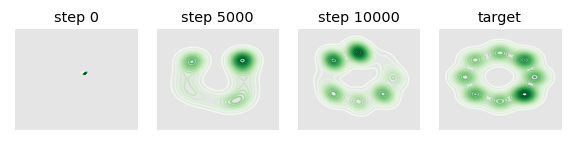
(a) Results of the standard GAN.

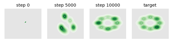
(b) Results of the standard GAN with the proposed morphing during testing.

Figure 5: More results of standard GAN in toy experiment.

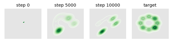
(a) Results of the MMD-GAN.

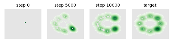
(b) Results of the MMD-GAN with the proposed morphing during testing.

Figure 6: More results of MMD-GAN in toy experiment.

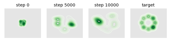
(a) Results of the EBM with 10-step sampling.

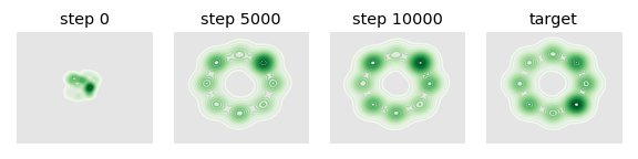
(b) Results of the EBM with 30-step sampling.

Figure 7: More results of EBM in toy experiment.

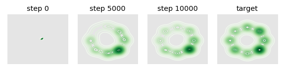
(a) Results of the proposed method.

Figure 8: More results of the proposed model in toy experiment.

Appendix G More Results on Refining AFHQ Generation

Table 10: Plug-and-play StyleGAN2+ADA on AFHQ ($512\times 512$)

Cat Dog Wild Models FID $(\downarrow)$ FID $(\downarrow)$ FID $(\downarrow)$ StyleGAN2+ADA $3.55$ $7.40$ $3.05$ Ours $\mathbf{3.17}$ $\mathbf{7.31}$ $\mathbf{2.99}$

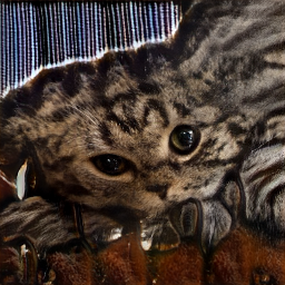
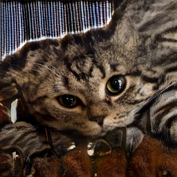
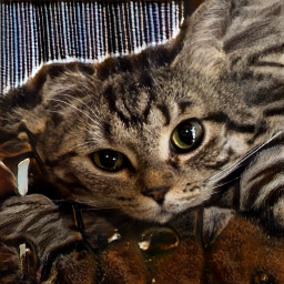
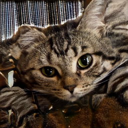
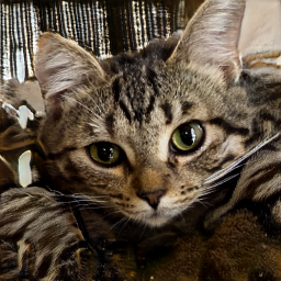
(a) Random seed 301

(b) Random seed 869

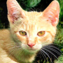
(c) Random seed 1348

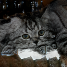
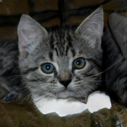
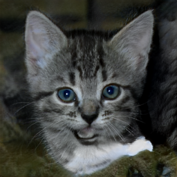
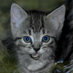
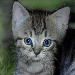
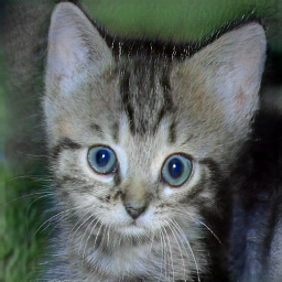
(d) Random seed 1469

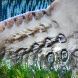
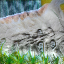
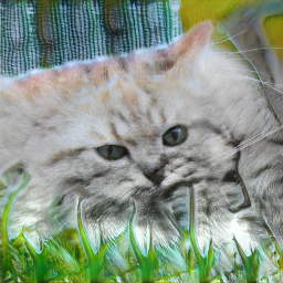
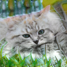
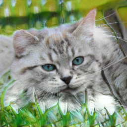
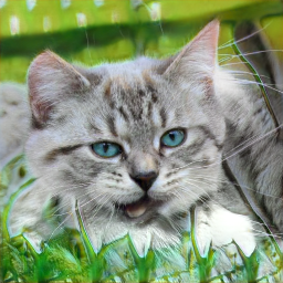
(e) Random seed 1645

Figure 9: More results of refining StyleGAN2+ADA pre-trained model on AFHQ Cat ($512\times 512$).

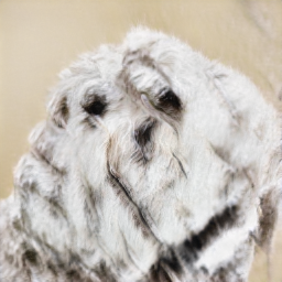
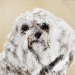
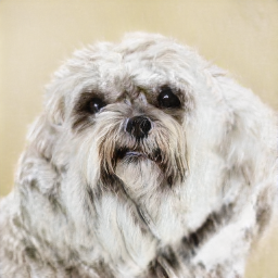
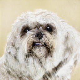
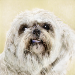
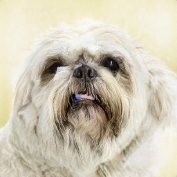
(a) Random seed 234

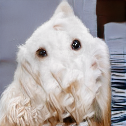
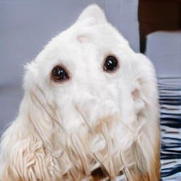
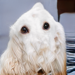
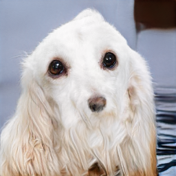
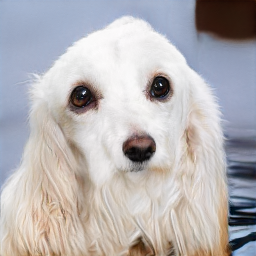
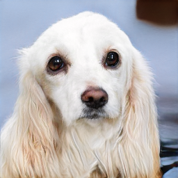
(b) Random seed 293

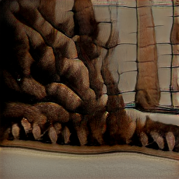
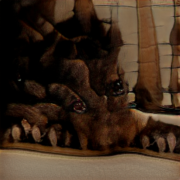
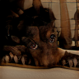
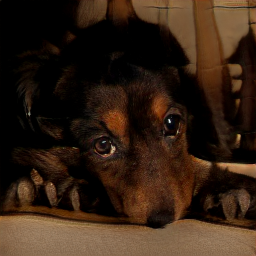
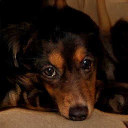
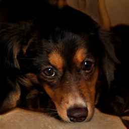
(c) Random seed 338

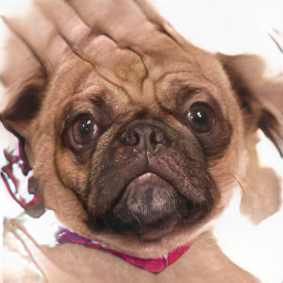
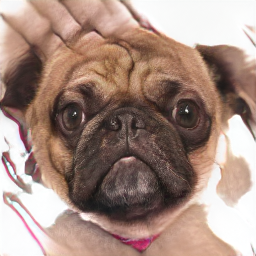
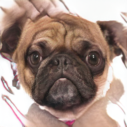
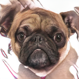
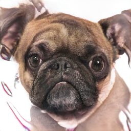
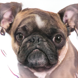
(d) Random seed 353

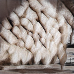
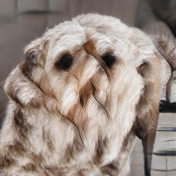
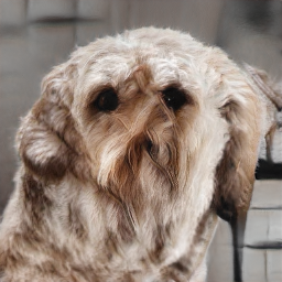
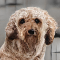
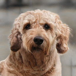
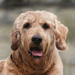
(e) Random seed 496

Figure 10: More results of refining StyleGAN2+ADA pre-trained model on AFHQ Dog ($512\times 512$).

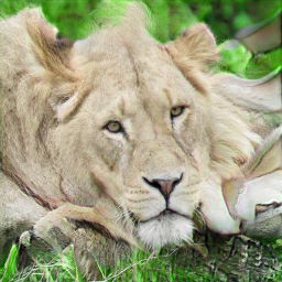
(a) Random seed 541

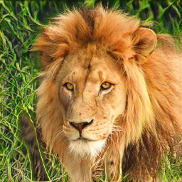
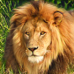
(b) Random seed 829

Figure 11: Results of refining StyleGAN2+ADA pre-trained model on AFHQ Wild ($512\times 512$).

Appendix H More Results on Image Generation

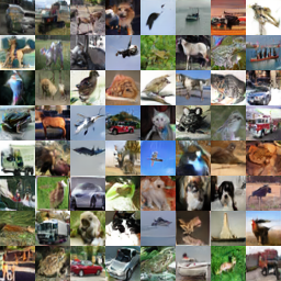
(a) CIFAR-10 ($32\times 32$)

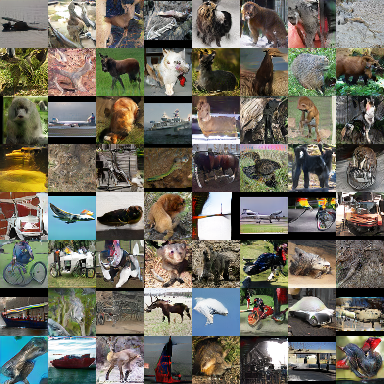
(b) STL-10 ($48\times 48$)

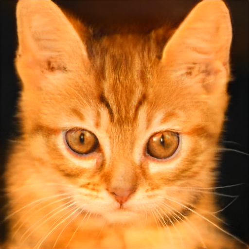
(c) AFHQ Cat ($512\times 512$)

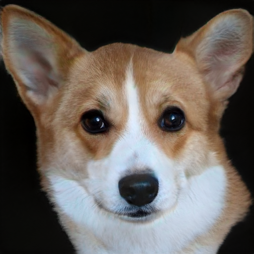
(d) AFHQ Dog ($512\times 512$)

Figure 12: Generated images using the proposed method.

Table 11: FID results of the proposed method on STL-10.

Steps Functional Langevin KL RKL JS SH Trained without morphing 0 $33.50\pm 0.13$ 10 $27.72\pm 0.16$ $24.20\pm 0.08$ $28.01\pm 0.10$ $24.49\pm 0.09$ $25.01\pm 0.06$ 20 $27.28\pm 0.05$ $23.18\pm 0.04$ $26.41\pm 0.08$ $23.33\pm 0.08$ $23.29\pm 0.04$ 30 $27.80\pm 0.09$ $22.36\pm 0.07$ $24.61\pm 0.06$ $22.36\pm 0.07$ $22.50\pm 0.05$ 40 $27.28\pm 0.08$ $22.82\pm 0.05$ $24.32\pm 0.12$ $\mathbf{22.15\pm 0.07}$ $22.27\pm 0.12$ Trained with 5-step morphing 0 $32.82\pm 0.07$ 10 $26.26\pm 0.09$ $22.22\pm 0.09$ $24.15\pm 0.11$ $23.81\pm 0.09$ $23.37\pm 0.08$ 20 $26.61\pm 0.07$ $21.52\pm 0.13$ $23.06\pm 0.10$ $22.56\pm 0.06$ $22.17\pm 0.06$ 30 $27.16\pm 0.12$ $\mathbf{21.40\pm 0.05}$ $22.69\pm 0.06$ $21.77\pm 0.07$ $21.69\pm 0.07$ 40 $26.76\pm 0.15$ $21.49\pm 0.07$ $22.65\pm 0.10$ $21.91\pm 0.14$ $21.89\pm 0.03$

Appendix I More Results of Image Translation

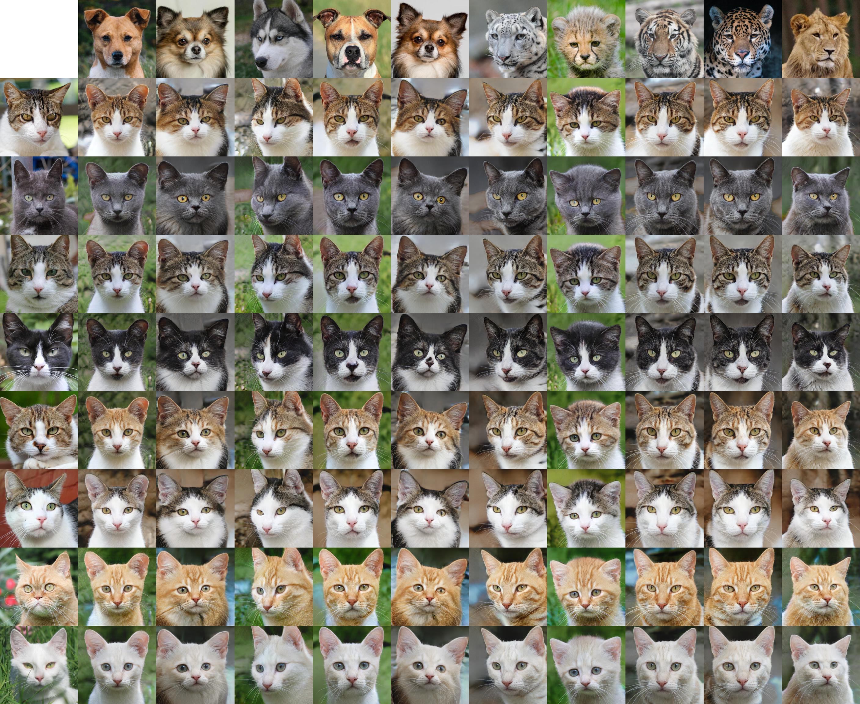
Figure 13: More results of image translation on AFHQ dataset. The first row images are source images, the first column images are reference images.

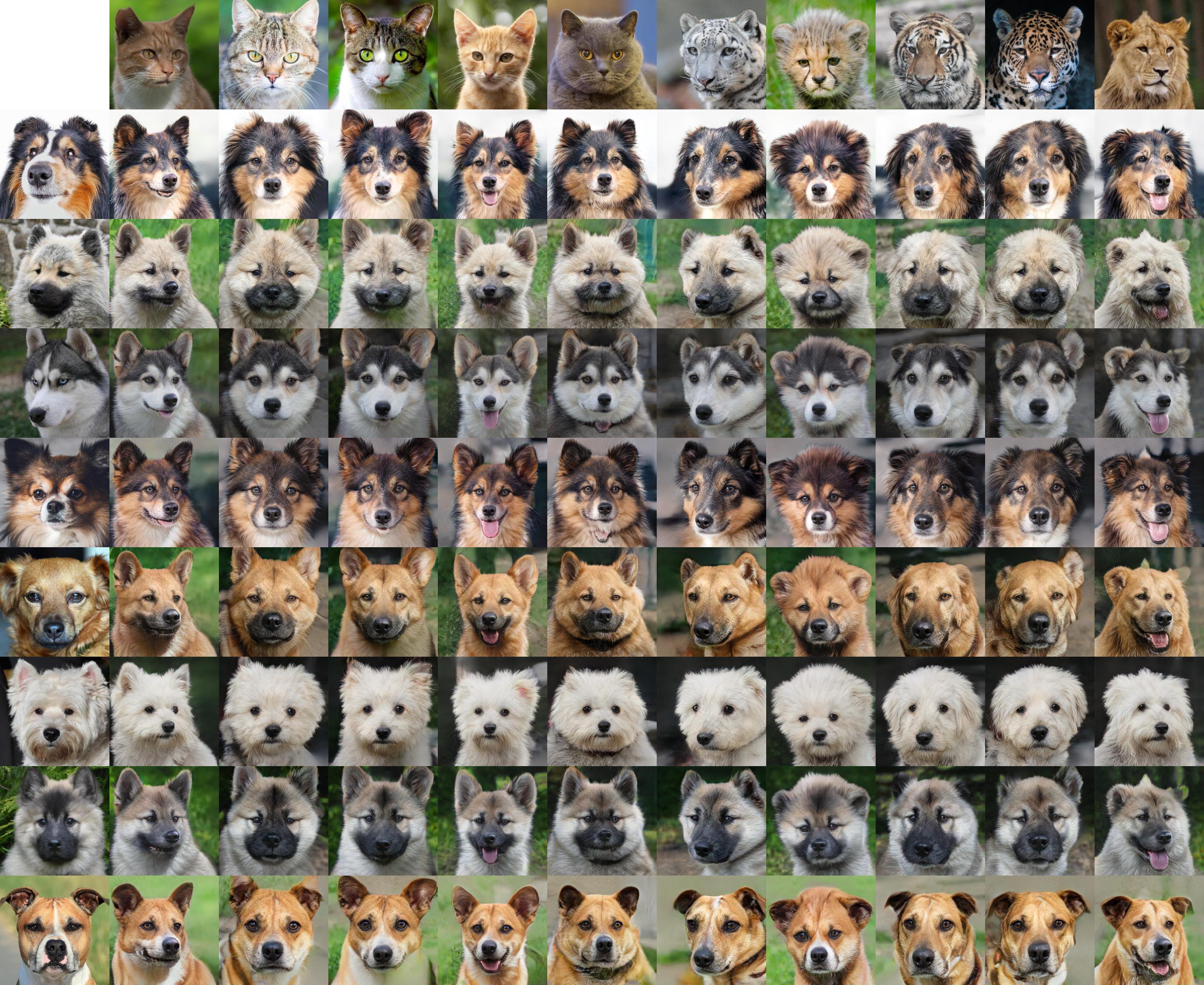
Figure 14: More results of image translation on AFHQ dataset. The first row images are source images, the first column images are reference images.

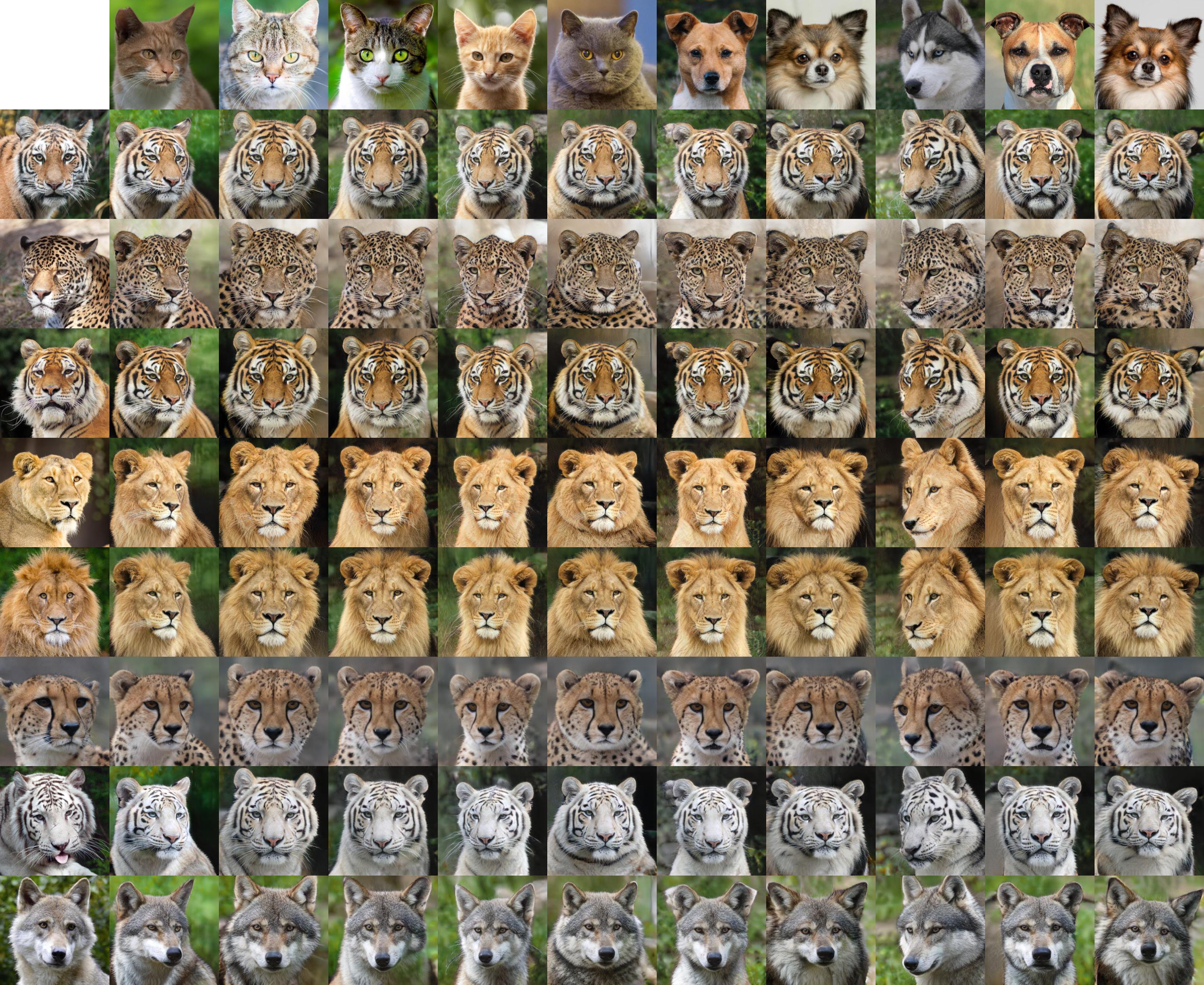
Figure 15: More results of image translation on AFHQ dataset. The first row images are source images, the first column images are reference images.

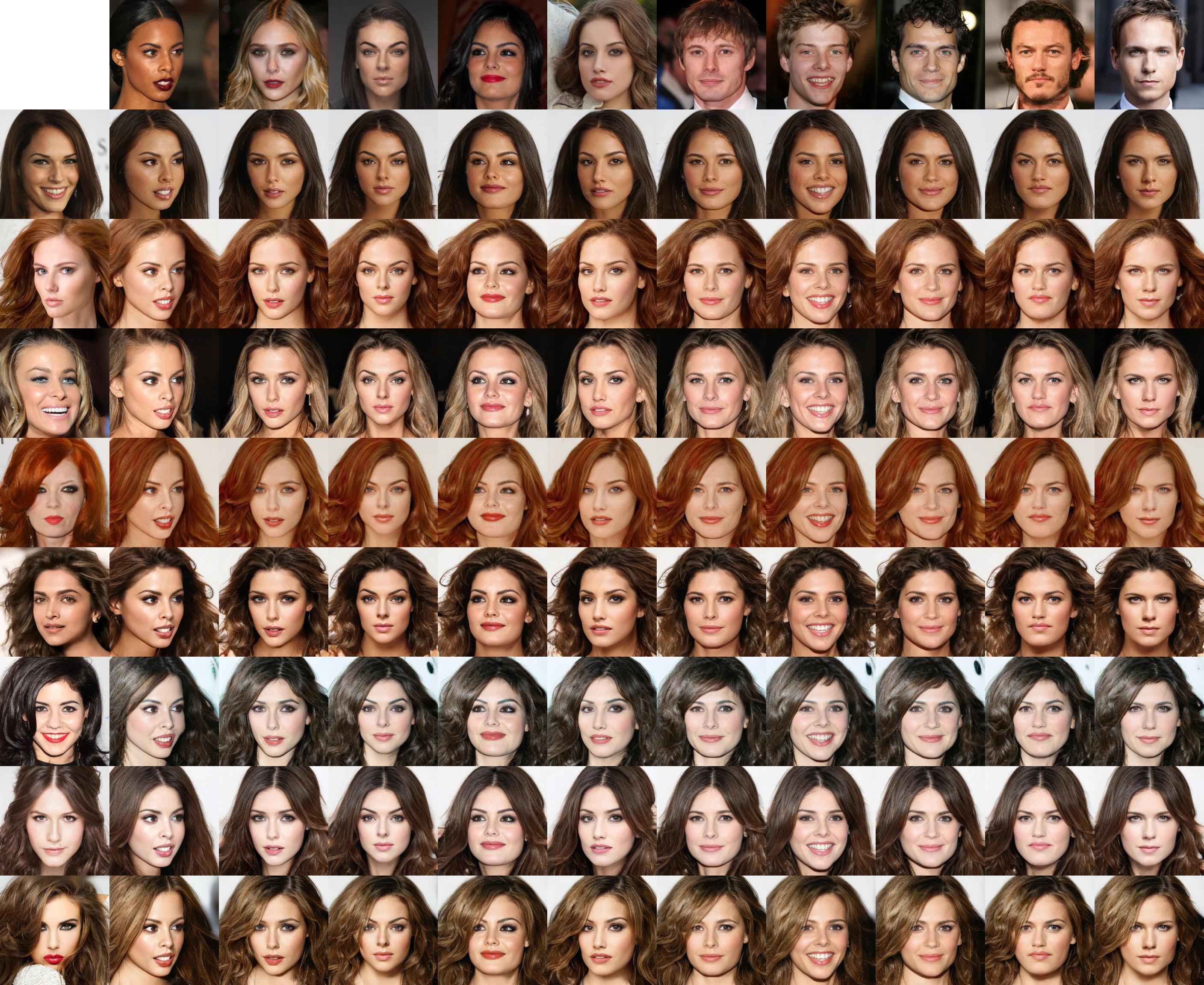
Figure 16: More results of image translation on CelebA-HQ dataset. The first row images are source images, the first column images are reference images.

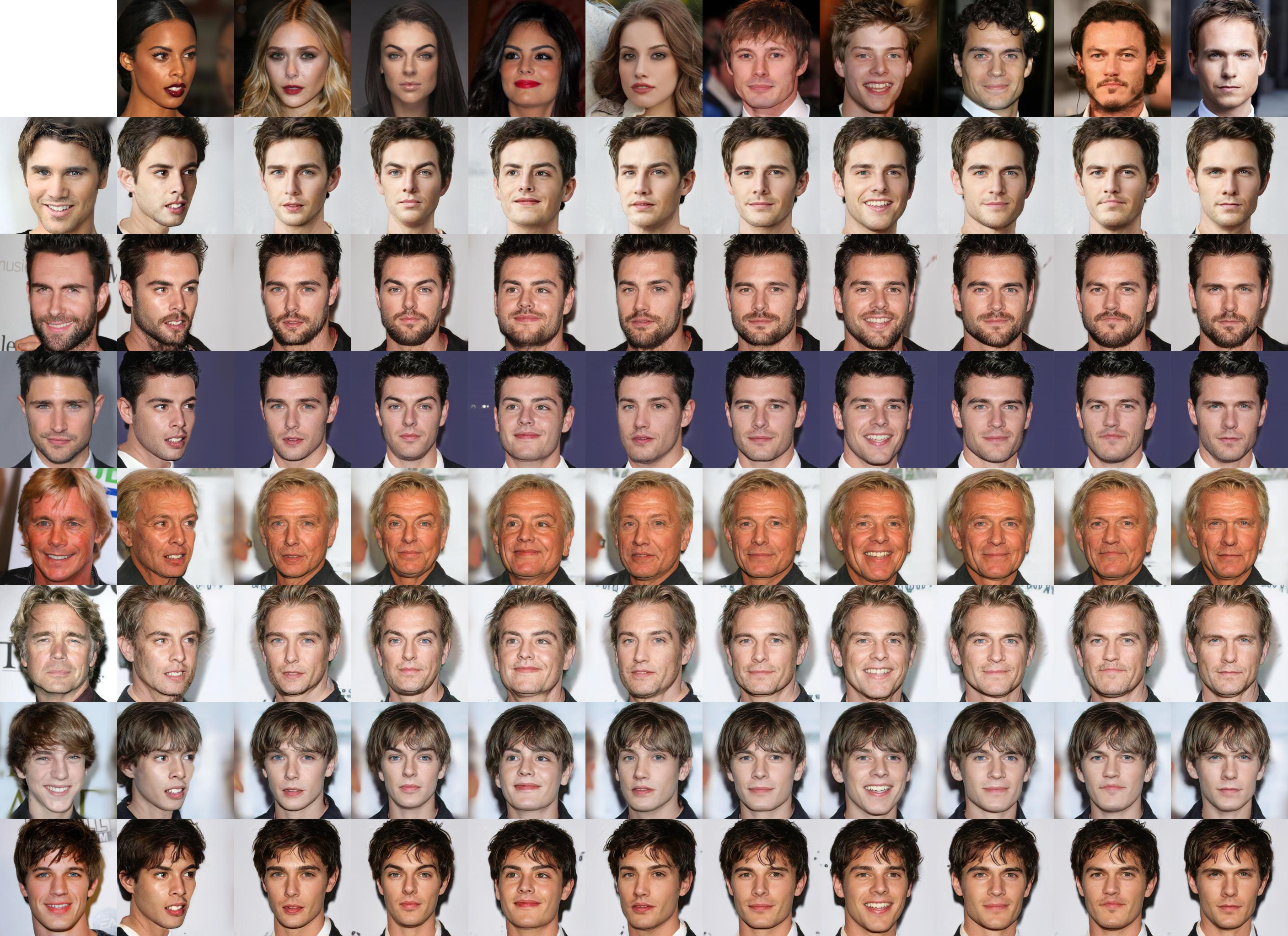
Figure 17: More results of image translation on CelebA-HQ dataset. The first row images are source images, the first column images are reference images.

References

• Ambrosio et al. (2008) Ambrosio, L., Gigli, N., and Savaré, G. Gradient flows: in metric spaces and in the space of probability measures. Springer Science & Business Media, 2008.
• Ansari et al. (2020) Ansari, A. F., Ang, M. L., and Soh, H. Refining deep generative models via wasserstein gradient flows. arXiv preprint arXiv:2012.00780, 2020.
• Arbel et al. (2018) Arbel, M., Sutherland, D., Bińkowski, M., and Gretton, A. On gradient regularizers for mmd gans. In Advances in neural information processing systems, pp. 6700–6710, 2018.
• Arbel et al. (2020) Arbel, M., Zhou, L., and Gretton, A. Kale: When energy-based learning meets adversarial training. ArXiv, abs/2003.05033, 2020.
• Arjovsky et al. (2017) Arjovsky, M., Chintala, S., and Bottou, L. Wasserstein generative adversarial networks. In International conference on machine learning, pp. 214–223. PMLR, 2017.
• Bilal (2020) Bilal, A. Small-time expansion of the fokker–planck kernel for space and time dependent diffusion and drift coefficients. Journal of Mathematical Physics, 61(6):061517, Jun 2020. ISSN 1089-7658. doi: 10.1063/5.0006009. URL http://dx.doi.org/10.1063/5.0006009.
• Brock et al. (2018) Brock, A., Donahue, J., and Simonyan, K. Large scale gan training for high fidelity natural image synthesis. In International Conference on Learning Representations, 2018.
• Carrillo & Toscani (1998) Carrillo, J. A. and Toscani, G. Exponential convergence toward equilibrium for homogeneous fokker–planck-type equations. Mathematical methods in the applied sciences, 21(13):1269–1286, 1998.
• Che et al. (2020) Che, T., Zhang, R., Sohl-Dickstein, J., Larochelle, H., Paull, L., Cao, Y., and Bengio, Y. Your gan is secretly an energy-based model and you should use discriminator driven latent sampling. arXiv preprint arXiv:2003.06060, 2020.
• Chizat et al. (2020) Chizat, L., Roussillon, P., Léger, F., Vialard, F.-X., and Peyré, G. Faster wasserstein distance estimation with the sinkhorn divergence. Advances in Neural Information Processing Systems, 33, 2020.
• Choi et al. (2020) Choi, Y., Uh, Y., Yoo, J., and Ha, J. W. Stargan v2: Diverse image synthesis for multiple domains. In 2020 IEEE/CVF Conference on Computer Vision and Pattern Recognition (CVPR), pp.  8185–8194, 2020. doi: 10.1109/CVPR42600.2020.00821.
• Cuturi (2013) Cuturi, M. Sinkhorn distances: Lightspeed computation of optimal transport. Advances in neural information processing systems, 26:2292–2300, 2013.
• Du & Mordatch (2019) Du, Y. and Mordatch, I. Implicit generation and modeling with energy based models. In Wallach, H., Larochelle, H., Beygelzimer, A., d'Alché-Buc, F., Fox, E., and Garnett, R. (eds.), Advances in Neural Information Processing Systems 32, pp.  3608–3618. Curran Associates, Inc., 2019.
• Gao et al. (2020) Gao, C., Chen, Y., Liu, S., Tan, Z., and Yan, S. Adversarialnas: Adversarial neural architecture search for gans. In Proceedings of the IEEE/CVF Conference on Computer Vision and Pattern Recognition (CVPR), June 2020.
• Genevay et al. (2018) Genevay, A., Peyré, G., and Cuturi, M. Learning generative models with sinkhorn divergences. In International Conference on Artificial Intelligence and Statistics, pp.  1608–1617. PMLR, 2018.
• Gong et al. (2019) Gong, X., Chang, S., Jiang, Y., and Wang, Z. Autogan: Neural architecture search for generative adversarial networks. In Proceedings of the IEEE/CVF International Conference on Computer Vision, pp.  3224–3234, 2019.
• Goodfellow et al. (2014) Goodfellow, I. J., Pouget-Abadie, J., Mirza, M., Xu, B., Warde-Farley, D., Ozair, S., Courville, A., and Bengio, Y. Generative adversarial nets. In Proceedings of the 27th International Conference on Neural Information Processing Systems-Volume 2, pp.  2672–2680, 2014.
• Grathowhl et al. (2020) Grathowhl, W., Kelly, J., Hashemi, M., Norouzi, M., Swersky, K., and Duvenaud, D. No mcmc for me: Amortized sampling for fast and stable training of energy-based models. arXiv preprint arXiv:2010.04230, 2020.
• Gulrajani et al. (2017) Gulrajani, I., Ahmed, F., Arjovsky, M., Dumoulin, V., and Courville, A. Improved training of wasserstein gans. In Proceedings of the 31st International Conference on Neural Information Processing Systems, pp.  5769–5779, 2017.
• Huang et al. (2018) Huang, X., Liu, M.-Y., Belongie, S., and Kautz, J. Multimodal unsupervised image-to-image translation. In Proceedings of the European conference on computer vision (ECCV), pp.  172–189, 2018.
• Itô (1951) Itô, K. On stochastic differential equations. Number 4. American Mathematical Soc., 1951.
• Jordan et al. (1998) Jordan, R., Kinderlehrer, D., and Otto, F. The variational formulation of the fokker–planck equation. SIAM journal on mathematical analysis, 29(1):1–17, 1998.
• Karras et al. (2020a) Karras, T., Aittala, M., Hellsten, J., Laine, S., Lehtinen, J., and Aila, T. Training generative adversarial networks with limited data. arXiv preprint arXiv:2006.06676, 2020a.
• Karras et al. (2020b) Karras, T., Laine, S., Aittala, M., Hellsten, J., Lehtinen, J., and Aila, T. Analyzing and improving the image quality of stylegan. In Proceedings of the IEEE/CVF Conference on Computer Vision and Pattern Recognition, pp.  8110–8119, 2020b.
• Kingma & Dhariwal (2018) Kingma, D. P. and Dhariwal, P. Glow: generative flow with invertible 1$\times$ 1 convolutions. In Proceedings of the 32nd International Conference on Neural Information Processing Systems, pp.  10236–10245, 2018.
• Kingma & Welling (2014) Kingma, D. P. and Welling, M. Auto-Encoding Variational Bayes. In 2nd International Conference on Learning Representations, ICLR 2014, Banff, AB, Canada, April 14-16, 2014, Conference Track Proceedings, 2014.
• Kumar et al. (2019) Kumar, R., Ozair, S., Goyal, A., Courville, A., and Bengio, Y. Maximum entropy generators for energy-based models, 2019.
• Lee et al. (2018) Lee, H.-Y., Tseng, H.-Y., Huang, J.-B., Singh, M., and Yang, M.-H. Diverse image-to-image translation via disentangled representations. In Proceedings of the European conference on computer vision (ECCV), pp.  35–51, 2018.
• Li et al. (2017) Li, C.-L., Chang, W.-C., Cheng, Y., Yang, Y., and Póczos, B. Mmd gan: Towards deeper understanding of moment matching network. In Advances in neural information processing systems, pp. 2203–2213, 2017.
• Li et al. (2019) Li, C.-L., Chang, W.-C., Mroueh, Y., Yang, Y., and Póczos, B. Implicit kernel learning. In The 22nd International Conference on Artificial Intelligence and Statistics, pp.  2007–2016. PMLR, 2019.
• Mao et al. (2019) Mao, Q., Lee, H.-Y., Tseng, H.-Y., Ma, S., and Yang, M.-H. Mode seeking generative adversarial networks for diverse image synthesis. In Proceedings of the IEEE/CVF Conference on Computer Vision and Pattern Recognition, pp.  1429–1437, 2019.
• Miyato et al. (2018) Miyato, T., Kataoka, T., Koyama, M., and Yoshida, Y. Spectral normalization for generative adversarial networks. In International Conference on Learning Representations, 2018.
• Nguyen et al. (2010) Nguyen, X., Wainwright, M. J., and Jordan, M. I. Estimating divergence functionals and the likelihood ratio by convex risk minimization. IEEE Transactions on Information Theory, 56(11):5847–5861, 2010.
• Nowozin et al. (2016) Nowozin, S., Cseke, B., and Tomioka, R. f-gan: training generative neural samplers using variational divergence minimization. In Proceedings of the 30th International Conference on Neural Information Processing Systems, pp.  271–279, 2016.
• Rahimi & Recht (2007) Rahimi, A. and Recht, B. Random features for large-scale kernel machines. In Proceedings of the 20th International Conference on Neural Information Processing Systems, pp.  1177–1184, 2007.
• Remes et al. (2017) Remes, S., Heinonen, M., and Kaski, S. Non-stationary spectral kernels. In Proceedings of the 31st International Conference on Neural Information Processing Systems, pp.  4645–4654, 2017.
• Rezende & Mohamed (2015) Rezende, D. and Mohamed, S. Variational inference with normalizing flows. In International Conference on Machine Learning, pp. 1530–1538. PMLR, 2015.
• Risken (1996) Risken, H. Fokker-planck equation. In The Fokker-Planck Equation, pp.  63–95. Springer, 1996.
• Roberts et al. (1996) Roberts, G. O., Tweedie, R. L., et al. Exponential convergence of langevin distributions and their discrete approximations. Bernoulli, 2(4):341–363, 1996.
• Samo & Roberts (2015) Samo, Y.-L. K. and Roberts, S. Generalized spectral kernels. arXiv preprint arXiv:1506.02236, 2015.
• Santambrogio (2016) Santambrogio, F. Euclidean, Metric, and Wasserstein gradient flows: an overview, 2016.
• Shawe-Taylor et al. (2004) Shawe-Taylor, J., Cristianini, N., et al. Kernel methods for pattern analysis. Cambridge university press, 2004.
• Song & Ermon (2019) Song, Y. and Ermon, S. Generative modeling by estimating gradients of the data distribution. In Proceedings of the 33rd Annual Conference on Neural Information Processing Systems, 2019.
• Tanaka (2019) Tanaka, A. Discriminator optimal transport. In Advances in Neural Information Processing Systems, pp. 6816–6826, 2019.
• Wang et al. (2018) Wang, W., Sun, Y., and Halgamuge, S. Improving mmd-gan training with repulsive loss function. In International Conference on Learning Representations, 2018.
• Wasserman (2006) Wasserman, L. All of Nonparametric Statistics (Springer Texts in Statistics). Springer-Verlag, Berlin, Heidelberg, 2006. ISBN 0387251456.
• Welling & Teh (2011) Welling, M. and Teh, Y. W. Bayesian learning via stochastic gradient langevin dynamics. In Proceedings of the 28th international conference on machine learning (ICML-11), pp.  681–688, 2011.
• Xie et al. (2020) Xie, J., Lu, Y., Gao, R., Zhu, S., and Wu, Y. Cooperative training of descriptor and generator networks. IEEE Transactions on Pattern Analysis and Machine Intelligence, 42:27–45, 2020.
• Yu et al. (2020) Yu, L., Song, Y., Song, J., and Ermon, S. Training deep energy-based models with f-divergence minimization. In International Conference on Machine Learning, pp. 10957–10967. PMLR, 2020.
• Zhang et al. (2019) Zhang, H., Zhang, Z., Odena, A., and Lee, H. Consistency regularization for generative adversarial networks. In International Conference on Learning Representations, 2019.
• Zhou et al. (2019) Zhou, Y., Chen, C., and Xu, J. Kernelnet: A data-dependent kernel parameterization for deep generative modeling. arXiv preprint arXiv:1912.00979, 2019.