Causal Inference under Network Interference with Noise

Abstract

Increasingly, there is a marked interest in estimating causal effects under network interference due to the fact that interference manifests naturally in networked experiments. However, network information generally is available only up to some level of error. We study the propagation of such errors to estimators of average causal effects under network interference. Specifically, assuming a four-level exposure model and Bernoulli random assignment of treatment, we characterize the impact of network noise on the bias and variance of standard estimators in homogeneous and inhomogeneous networks. In addition, we propose method-of-moments estimators for bias reduction where a minimal number of network replicates are available. We show our estimators are asymptotically normal and provide confidence intervals for quantifying the uncertainty in these estimates. We illustrate the practical performance of our estimators through simulation studies in British secondary school contact networks.

Keywords: Noisy network; Causal effect; Exposure model; Method-of-moments.

1 Introduction

In recent years, there has been an enormous interest in the assessment of treatment effects within networked systems. Naturally, interference (Cox and Cox, (1958)) cannot realistically be assumed away when doing experiments on networks. The outcome of one individual may be affected by the treatment assigned to other individuals, which violates the ‘stable unit treatment value assumption’ (SUTVA) (Neyman, (1923), Rubin, (1990)). As a result, much of what is considered standard in the traditional design of randomized experiments and the corresponding analysis for causal inference does not apply directly in this context.

Moreover, network information generally is available only up to some level of error, also known as network noise. For example, there is often measurement error associated with network constructions, where, by ‘measurement error’ we will mean true edges being observed as non-edges, and vice versa. Such edge noise occurs in self-reported contact networks where participants may not perceive and recall all contacts correctly (Smieszek et al., (2012)). It can also be found in biological networks (e.g., of gene regulatory relationships), which are often based on notions of association (e.g., correlation, partial correlation, etc.) among experimental measurements of gene activity levels that are determined by some form of statistical inference. We investigate how network noise impacts estimators of average causal effects under network interference and how to account for the noise.

1.1 Problem setup

We assume the observed graph is a noisy version of a true graph. Let $G=(V,E)$ be an undirected graph and $G^{\text{obs}}=(V,E^{\text{obs}})$ be the observed graph, where we assume that the vertex set $V$ is known. Denote the adjacency matrix of $G$ by $\bm{A}=(A_{i,j})_{N_{v}\times N_{v}}$ and that of $G^{\text{obs}}$ by $\tilde{\bm{A}}=(\tilde{A}_{i,j})_{N_{v}\times N_{v}}$. Hence $A_{i,j}=1$ if there is a true edge between the $i$-th vertex and the $j$-th vertex, and 0 otherwise, while $\tilde{A}_{i,j}=1$ if an edge is observed between the $i$-th vertex and the $j$-th vertex, and 0 otherwise. We assume throughout that $G$ and $G^{\text{obs}}$ are simple.

We express the marginal distributions of the $\tilde{A}_{i,j}$ in the form (Balachandran et al., (2017)):

$$\tilde{A}_{i,j}\sim\begin{cases}\text{Bernoulli}(\alpha_{i,j}),&\text{if }\{i,j\}\in E^{c},\\ \text{Bernoulli}(1-\beta_{i,j}),&\text{if }\{i,j\}\in E,\\ \end{cases}$$ (1.1)

where $E^{c}=\{\{i,j\}:i,j\in V;i<j\}\backslash E$. Drawing by analogy on the example of network construction based on hypothesis testing, $\alpha_{i,j}$ can be interpreted as the probability of a Type-I error on the (non)edge status for vertex pair $\{i,j\}\in E^{c}$, while $\beta_{i,j}$ is interpreted as the probability of Type-II error, for vertex pair $\{i,j\}\in E$. Our interest is in characterizing the manner in which the uncertainty in the $\tilde{A}_{i,j}$ propagates to estimators of average causal effects.

Let $z_{i}=1$ indicate that individual $i\in V$ received a given treatment. We will refer to $\bm{z}=(z_{1},\cdots,z_{N_{v}})^{\top}\in\{0,1\}^{N_{v}}$ as the treatment assignment vector. Let $p_{\bm{z}}=\mathbb{P}(\bm{Z}=\bm{z})$ be the probability that treatment assignment $\bm{z}$ is generated by the experimental design. Additionally, let $y_{i}(\bm{z})$ denote the outcome for individual $i$ under treatment assignment $\bm{z}$. In the worst case, there will be $2^{N_{v}}$ possible exposures for each of the $N_{v}$ individuals, making causal inference impossible. To avoid this situation, we adopt the notion of so-called exposure mappings, introduced by Aronow and Samii, (2017). We say that $i$ is exposed to condition $k=1,\ldots,K$ if $f(\bm{z},\bm{x}_{i})=c_{k}$, where $f$ is the exposure mapping, $\bm{z}$ is the treatment assignment vector, and $\bm{x}_{i}$ is a vector of additional information specific to individual $i$. Under interference, these authors offer a simple, four-level categorization of exposure ($K=4$) that we revisit here and throughout this paper. Taking the vector $\bm{x}_{i}$ to be the $i$th column of the adjacency matrix $\bm{A}$ (i.e., $\bm{x}_{i}=\bm{A}_{.i}$), they define

$$f(\bm{z},\bm{A}_{\cdot i})=\begin{cases}c_{11}\text{(Direct + Indirect Exposure)},&z_{i}I_{\{\bm{z}^{\top}\bm{A}_{\cdot i}>0\}}=1,\\ c_{10}\text{(Isolated Direct Exposure)},&z_{i}I_{\{\bm{z}^{\top}\bm{A}_{\cdot i}=0\}}=1,\\ c_{01}\text{(Indirect Exposure)},&(1-z_{i})I_{\{\bm{z}^{\top}\bm{A}_{\cdot i}>0\}}=1,\\ c_{00}\text{(No Exposure)},&(1-z_{i})I_{\{\bm{z}^{\top}\bm{A}_{\cdot i}=0\}}=1,\end{cases}$$ (1.2)

where the inner product $\bm{z}^{\top}\bm{A}_{\cdot i}$ is the number of treated neighbors of individual $i$.

In the general exposure mapping framework of Aronow and Samii, (2017), potential outcomes are dependent only on the exposure conditions for each unit. Suppose each individual $i$ has $K$ potential outcomes $y_{i}(c_{1}),\cdots,y_{i}(c_{K})$ and is exposed to one and only one condition. Then, define

$$\uptau(c_{k},c_{l})=\frac{1}{N_{v}}\sum_{i=1}^{N_{v}}\left[y_{i}(c_{k})-y_{i}(c_{l})\right]=\overline{y}(c_{k})-\overline{y}(c_{l})$$ (1.3)

to be the average causal contrast between exposure condition $k$ versus $l$. Consider again, for example, the exposure mapping function defined in (1.2). A natural set of contrasts is $\uptau(c_{01},c_{00})$, $\uptau(c_{10},c_{00})$, and $\uptau(c_{11},c_{00})$, which capture the average indirect treatment effect, the average direct treatment effect, and the average total treatment effect, respectively.

Now consider the problem of inference for causal effects under network interference. The Horvitz-Thompson framework accounts for unequal-probability sampling through the use of inverse probability weighting (Horvitz and Thompson, (1952)) and is adapted by Aronow and Samii, (2017) under exposure mappings. In noise-free networks, assuming all individuals have nonzero exposure probabilities for all exposure conditions, the estimator

$$\hat{\overline{y}}(c_{k})=\frac{1}{N_{v}}\Bigg{\{}\sum_{i=1}^{N_{v}}I_{\{f({\bm{Z}},{\bm{x}}_{i})=c_{k}\}}\frac{y_{i}(c_{k})}{p_{i}^{e}(c_{k})}\Bigg{\}}$$ (1.4)

is well-defined and unbiased for $\overline{y}(c_{k})$, where the exposure probabilities $p_{i}^{e}(c_{k})$ are defined as $\sum_{\bm{z}}p_{\bm{z}}I_{\{f({\bm{z}},{\bm{x}}_{i})=c_{k}\}}$. In turn, $\hat{\uptau}(c_{k},c_{l})=\hat{\overline{y}}(c_{k})-\hat{\overline{y}}(c_{l})$ is an unbiased estimator of $\uptau(c_{k},c_{l})$.

However, in noisy networks, some exposure levels will be misclassified. For example, in the four-level exposure model, for a node $i$, the expected confusion matrix for observed (rows) versus true (columns) exposures has the following form

$$\bm{P}_{i}\coloneqq\begin{bmatrix}P_{i}(\tilde{c}_{11},c_{11})&P_{i}(\tilde{c}_{11},c_{10})&0&0\\ P_{i}(\tilde{c}_{10},c_{11})&P_{i}(\tilde{c}_{10},c_{10})&0&0\\ 0&0&P_{i}(\tilde{c}_{01},c_{01})&P_{i}(\tilde{c}_{01},c_{00})\\ 0&0&P_{i}(\tilde{c}_{00},c_{01})&P_{i}(\tilde{c}_{00},c_{00})\\ \end{bmatrix},$$ (1.5)

where $\tilde{c}_{k}$ represents the exposure level in observed networks and $P_{i}(\tilde{c}_{k},c_{l})=\mathbb{E}[I_{\{f({\bm{Z}},\tilde{\bm{A}}_{i})=c_{k}\}}I_{\{f({\bm{Z}},{\bm{A}}_{i})=c_{l}\}}]$. The two off-diagonal blocks are equal to 0, since network noise does not affect treatment status. The four symbols $P_{i}(\tilde{c}_{k},c_{l}),k\neq l$ are cases where exposure levels are misclassified. In the general exposure mapping framework, the estimators (1.4) for $\overline{y}(c_{k})$ are in fact

$$\tilde{\overline{y}}_{A\&S}(c_{k})=\frac{1}{N_{v}}\sum_{i=1}^{N_{v}}I_{\{\tilde{p}_{i}^{e}(c_{k})>0\}}I_{\{f({\bm{Z}},{\tilde{\bm{X}}}_{i})=c_{k}\}}\frac{1}{\tilde{p}_{i}^{e}(c_{k})}\Bigg{\{}\sum_{l=1}^{K}y_{i}(c_{l})\ I_{\{f({\bm{Z}},{\bm{x}}_{i})=c_{l}\}}\Bigg{\}},$$ (1.6)

where $\tilde{\bm{X}}_{i}$ is a noisy version of $\bm{x}_{i}$, and $\tilde{p}_{i}^{e}(c_{k})=\sum_{\bm{z}}p_{\bm{z}}I_{\{f({\bm{z}},\tilde{\bm{X}}_{i})=c_{k}\}}$. From (1.6), we can see that the errors introduced into this estimator by network noise come in two forms: incorrect exposure probabilities and misclassified exposure levels.

In this paper, we will address the following important questions. First, what is the impact of ignoring network noise? Second, how can we account for network noise?

1.2 Related literature

Awareness of interference goes back at least 100 years (e.g., Ross, (1916)), and its impact on standard theory and methods has been studied previously in certain specific contexts, including interference localized to an individual across different rounds of treatment in clinical trials with crossover designs (Grizzle, (1965)), interference based on spatial proximity of treated units (Kempton and Lockwood, (1984)) and interference within blocks (Hudgens and Halloran, (2008)). For network interference, an assumption that has gained traction is that the causal effects can be passed along edges in the network. A highly studied assumption is to assume that unit outcomes are only impacted by their neighbors in the network (Manski, (2013); Athey et al., (2018)). Researchers have recently developed frameworks for estimating average unit-level causal effects under network interference. For example, Aronow and Samii, (2017) provided unbiased estimators of average unit-level causal effects induced by treatment exposure. Sussman and Airoldi, (2017) proposed minimum integrated variance linear unbiased estimators with respect to a distribution on the potential outcomes.

Extensive work regarding uncertainty analysis has been done in causal inference without the network structure or interference. Many studies have explored the effects of uncertainty in propensity scores on causal inference. For instance, there have been efforts to develop Bayesian propensity score estimators to incorporate such uncertainties into causal inference (e.g., An, (2010), Alvarez and Levin, (2014)). And there are some studies on the properties for particular matching estimators for average causal effects (e.g., Abadie and Imbens, (2006), Schafer and Kang, (2008)). But, to our best knowledge, there has been little attention to date given towards uncertainty analysis of estimators for average causal effects under network interference. Exceptions include a Bayesian procedure which accounts for network uncertainty and relies on a linear response assumption to increase estimation precision (Toulis and Kao, (2013)), and structure learning techniques to estimate causal effects under data dependence induced by a network represented by a chain graph model, when the structure of this dependence is not known a priori (Bhattacharya et al., (2019)).

As remarked above, there appears to be little in the way of a formal and general treatment of the error propagation problem in estimators of average causal effects under network interference. However, there are several areas in which the probabilistic or statistical treatment of uncertainty enters prominently in network analysis. Model-based approaches include statistical methodology for predicting network topology or attributes with models that explicitly include a component for network noise (Jiang et al., (2011), Jiang and Kolaczyk, (2012)), the ‘denoising’ of noisy networks (Chatterjee et al., (2015)), the adaptation of methods for vertex classification using networks observed with errors (Priebe et al., (2015)), a regression model on network-linked data that is based on a flexible network effect assumption and is robust to errors in the network structure (Le and Li, (2020)), and a general Bayesian framework for reconstructing networks from observational data (Young et al., (2020)). The other common approach to network noise is based on a ‘signal plus noise’ perspective. For example, Balachandran et al., (2017) introduced a simple model for noisy networks that, conditional on some true underlying network, assumes we observe a version of that network corrupted by an independent random noise that effectively flips the status of (non)edges. Later, Chang et al., (2020) developed method-of-moments estimators for the underlying rates of error when replicates of the observed network are available. In a somewhat different direction, uncertainty in network construction due to sampling has also been studied in some depth. See, for example, Kolaczyk, (2009, Chapter 5) or Ahmed et al., (2014) for surveys of this area. However, in that setting, the uncertainty arises only from sampling—the subset of vertices and edges obtained through sampling are typically assumed to be observed without error.

1.3 Our contributions and organization of the paper

Our contribution in this paper is to quantify how network errors propagate to standard estimators of average causal effects under network interference, and to provide new estimators for average causal effects when replicates of the observed network are available. Adopting the noise model proposed by Balachandran et al., (2017), we characterize the impact of network noise on the bias and variance of standard estimators (Aronow and Samii, (2017)) under a four-level exposure model and Bernoulli random assignment of treatment, and we illustrate the asymptotic behaviors on networks for varying degree distributions. Additionally, we propose method-of-moments estimators of average causal effects that are asymptotically normal (as the number of vertices increases to infinity), when replicates of the observed network are available. Numerical simulation in the context of social contact networks in British secondary schools suggests that high accuracy is possible for networks of even modest size.

The organization of this paper is as follows. In Section 2 we present the bias and variance of standard estimators in noisy networks under a four-level exposure model and Bernoulli random assignment of treatment. Section 3 contains our proposed method-of-moments estimators for the true average causal effects. Numerical illustrations are reported in Section 4. Finally, we conclude in Section 5 with a discussion of future directions for this work. All proofs are relegated to supplementary materials.

2 Impact of ignoring network noise

In this section, we characterize the impact of network noise on biases and variances of standard estimators under a four-level exposure model and Bernoulli random assignment of treatment. Specifically, we show results for two typical classes of networks: homogeneous and inhomogeneous. By the term homogeneous we mean the degrees follow a zero-truncated Poisson distribution, and by inhomogeneous, the degrees follow a Pareto distribution with an exponential cutoff (Clauset et al.,, 2009). Note that many real networks present a bounded scale-free behavior with a connectivity cut-off due to the finite size of the network or to the presence of constraints limiting the addition of new links in an otherwise infinite network (Amaral et al., (2000)). The exponential cutoff is most widely used.

2.1 Network settings and assumptions

We consider two typical classes of networks: homogeneous and inhomogeneous. The formal definitions are as follows.

Homogeneous network setting

The degree distribution of $G$ is a zero-truncated Poisson distribution with mean $\bar{d}$.

Inhomogeneous network setting

The degree distribution of $G$ is a Pareto distribution with an exponential cutoff with rate $\lambda$, shape $\zeta$, lower bound $d_{L}$, upper bound $N_{v}-1$ and mean $\bar{d}$.

Remark 1

The degree distribution is the probability distribution of the degrees over the whole network.

Remark 2

Note that $\bar{d}$, $\lambda$ and $d_{L}$ depend on $N_{v}$. For notational simplicity, we omit $N_{v}$.

Remark 3

In the inhomogeneous network setting, by the definition of Pareto distribution with an exponential cutoff, the parameters $\lambda$, $\zeta$, $d_{L}$, $\bar{d}$ and $N_{v}$ satisfy the equation

$$\bar{d}=\int_{d_{L}}^{N_{v}-1}x\cdot e^{-\lambda x}x^{-(\zeta+1)}dx\Big{/}\int_{d_{L}}^{N_{v}-1}e^{-\lambda x}x^{-(\zeta+1)}dx.$$

Here we focus on a general formulation of the problem in which we make the following assumptions on networks and the treatment assignment.

Assumption 1 (Constant marginal error probabilities)

Assume that
$\alpha_{i,j}=\alpha$ and $\beta_{i,j}=\beta$ for all $i<j$, so the marginal error probabilities are $\mathbb{P}(\tilde{A}_{i,j}=0|A_{i,j}=1)=\beta$ and $\mathbb{P}(\tilde{A}_{i,j}=1|A_{i,j}=0)=\alpha$.

Assumption 2 (Independent noise)

The random variables $\tilde{A}_{i,j}$, for all $i<j$, are conditionally independent given $A_{i,j}$.

Assumption 3 (Large Graphs)

The number of vertices $N_{v}\rightarrow\infty$.

In Assumption 1, we assume that both $\alpha$ and $\beta$ remain constant over different edges. Under Assumptions 1 and 2, the distribution of $\tilde{d}_{i}$ is

$$\tilde{d}_{i}=\sum_{j=1}^{N_{v}}\tilde{A}_{j,i}\sim\text{Binomial}(N_{v}-1-d_{i},\alpha)+\text{Binomial}(d_{i},1-\beta).$$

Assumption 3 reflects both the fact that the study of large graphs is a hallmark of modern applied work in complex networks and, accordingly, our desire to understand asymptotic behaviors of estimators for average causal effects and provide concise descriptions in terms of biases and variances for large graphs.

Assumption 4

Individuals are assigned treatment independently with probability $p$ satisfying $p=o(1)$, $p=\omega(1/N_{v})$, $\bar{d}=\Theta(1/p)$. Letting $C_{ij}$ denote the number of common neighbors between vertices $i$ and $j$ in $G$, $\sum_{i=1}^{N_{v}}\sum_{j\neq i}^{N_{v}}I_{\{C_{ij}=0\}}\sim N_{v}^{2}$. Finally, the potential outcomes are bounded, $|y_{i}(c_{k})|\leq c<\infty$, for all values $i$ and $c_{k}$, where $c$ is a constant.

Assumption 4 entails that, as $N_{v}$ grows, the expected number of treated individuals also grows but is dominated by $N_{v}$ asymptotically. And the average number of treated neighbors is bounded. The amount of vertex pairs having common neighbors is also limited in scope as $N_{v}$ grows which ensures a sufficiently large set of independent exposures. Assumption 4 is an assumption used in proving the consistency of $\hat{\uptau}(c_{k},c_{l})$ in noise-free homogeneous and inhomogeneous networks. See Appendix 8.1 for details.

Assumption 5

$1-\beta=\Omega(1)$, $\alpha=\Theta(1/(pN_{v}))$, and $\alpha=o(p)$.

Remark 4

Note that $\alpha$ and $\beta$ can be constants or $o(1)$ as $N_{v}\rightarrow\infty$. For notational simplicity, we omit $N_{v}$.

Remark 5

Assumption 5 implies $p=\omega(1/\sqrt{N_{v}})$, which is consistent with Assumption 4.

By making assumptions on the underlying rates of error $\alpha$ and $\beta$, we will see that regularity conditions hold for noisy homogeneous and inhomogeneous networks in Appendix 8.2 .

2.2 Biases of standard estimators in noisy networks

Assuming a four-level exposure model and Bernoulli random assignment of treatment, we quantify the biases of standard estimators in homogeneous and inhomogeneous network settings. We begin with the following general result.

Theorem 1

Assume a four-level exposure model and Bernoulli random assignment of treatment with probability $p$. Under Assumptions 1 – 3, 5, $p=o(1)$, $p=\omega(1/N_{v})$ and the potential outcomes are bounded, we have

$$\text{Bias}\Big{[}\tilde{\overline{y}}_{A\&S}(c_{11})\Big{]}= \ -\frac{1}{N_{v}}\sum_{i=1}^{N_{v}}\frac{(1-p)^{d_{i}}\big{[}1-(1-\alpha p)^{N_{v}-1-d_{i}}\big{]}}{1-(1-\alpha p)^{N_{v}-1-d_{i}}(1-(1-\beta)p)^{d_{i}}}\ \uptau_{i}(c_{11},c_{10})+o(1),$$

$$\text{Bias}\Big{[}\tilde{\overline{y}}_{A\&S}(c_{10})\Big{]}= \ \frac{1}{N_{v}}\sum_{i=1}^{N_{v}}\big{[}1-(1-\beta p)^{d_{i}}\big{]}\ \uptau_{i}(c_{11},c_{10}),$$

$$\text{Bias}\Big{[}\tilde{\overline{y}}_{A\&S}(c_{01})\Big{]}= \ -\frac{1}{N_{v}}\sum_{i=1}^{N_{v}}\frac{(1-p)^{d_{i}}\big{[}1-(1-\alpha p)^{N_{v}-1-d_{i}}\big{]}}{1-(1-\alpha p)^{N_{v}-1-d_{i}}(1-(1-\beta)p)^{d_{i}}}\ \uptau_{i}(c_{01},c_{00})+o(1),$$

$$\text{Bias}\Big{[}\tilde{\overline{y}}_{A\&S}(c_{00})\Big{]}= \ \frac{1}{N_{v}}\sum_{i=1}^{N_{v}}\big{[}1-(1-\beta p)^{d_{i}}\big{]}\ \uptau_{i}(c_{01},c_{00}),$$

as $N_{v}\rightarrow\infty$, where $\uptau_{i}(c_{k},c_{l})=y_{i}(c_{k})-y_{i}(c_{l})$ and $d_{i}$ is the degree of the $i$-th vertex in the noise-free network $G$.

Theorem 1 then directly leads to the following corollary in homogeneous and inhomogeneous network settings.

Corollary 1 (Homogeneous and inhomogeneous)

Assume a four-level exposure model and Bernoulli random assignment of treatment with $p$. In both homogeneous and inhomogeneous network settings, under Assumptions 1 – 3, 5, $p=o(1)$, $p=\omega(1/N_{v})$ and the potential outcomes are bounded, the bias statement in Theorem 1 holds.

The proof of Theorem 1 is in supplementary material C. Corollary 1 directly follows from Theorem 1.

The above results show that biases of standard estimators in homogeneous and inhomogeneous network settings have the same expressions. Biases of $\tilde{\overline{y}}_{A\&S}(c_{11})$ and $\tilde{\overline{y}}_{A\&S}(c_{01})$ depend on both $\alpha$ and $\beta$, while biases of $\tilde{\overline{y}}_{A\&S}(c_{10})$ and $\tilde{\overline{y}}_{A\&S}(c_{00})$ only depend on $\beta$. Biases of $\tilde{\overline{y}}_{A\&S}(c_{11})$ and $\tilde{\overline{y}}_{A\&S}(c_{10})$ are related to $\uptau(c_{11},c_{10})$. And biases of $\tilde{\overline{y}}_{A\&S}(c_{01})$ and $\tilde{\overline{y}}_{A\&S}(c_{00})$ are related to $\uptau(c_{01},c_{00})$. These relationships follow because the network noise affects observed edges but not treatment status.

In proving these results, we also necessarily obtain an understanding of estimation bias for causal effects at the level of individuals, which we summarize here. Let $\tilde{y}_{A\&S,i}(c_{k})$ denote the Aronow and Samii estimator for $y_{i}(c_{k})$ in noisy networks, which corresponds to the $i$-th element of $\tilde{\overline{y}}_{A\&S}(c_{k})$ in (1.6). We summarize in the following table the asymptotic biases of $\tilde{y}_{A\&S,i}(c_{k})$ for high (top row) and low (bottom row) degree nodes.

Table 2.1: The asymptotic biases of $\tilde{y}_{A\&S,i}(c_{k})$ for high (top row) and low (bottom row) degree nodes.

	$\text{Bias}[\tilde{y}_{A\&S,i}(c_{11})]$	$\text{Bias}[\tilde{y}_{A\&S,i}(c_{10})]$	$\text{Bias}[\tilde{y}_{A\&S,i}(c_{01})]$	$\text{Bias}[\tilde{y}_{A\&S,i}(c_{00})]$
$d_{i}=\omega(1/p)$	$o(1)$	$\uptau_{i}(c_{11},c_{10})$	$o(1)$	$\uptau_{i}(c_{01},c_{00})$
$d_{i}=o(1/p)$	$-\uptau_{i}(c_{11},c_{10})$	$o(1)$	$-\uptau_{i}(c_{01},c_{00})$	$o(1)$

We see that there are four cases where $\tilde{y}_{A\&S,i}(c_{k})$ is asymptotically unbiased. The reason is that the corresponding entries in the expected confusion matrix (1.5) go to 0. For the other four cases, the corresponding entries in the expected confusion matrix approach 1, which leads to nontrivial biases. Note that the asymptotic biases of $\tilde{y}_{A\&S,i}(c_{k})$ is between 0 and the corresponding $\pm\uptau_{i}(c_{k},c_{l})$ when $d_{i}=\Theta(1/p)$.

2.3 Variances of standard estimators in noisy networks

We analyze the variances of standard estimators in homogeneous and inhomogeneous network settings.

Theorem 2 (Homogeneous)

Assume a four-level exposure model and Bernoulli random assignment of treatment with probability $p$. In the homogeneous network setting, under Assumptions 1 - 5, for all $c_{k}$, we have $\text{Var}[\tilde{\overline{y}}_{A\&S}(c_{k})]=o(1)$ as $N_{v}\rightarrow\infty$.

Theorem 3 (Inhomogeneous)

Assume a four-level exposure model and Bernoulli random assignment of treatment with probability $p$. In the inhomogeneous network setting, under Assumptions 1 - 5, $\lambda=\Theta(p)$ and $\lambda>p$, we have $\text{Var}[\tilde{\overline{y}}_{A\&S}(c_{k})]=o(1)$ for all $c_{k}$ as $N_{v}\rightarrow\infty$.

Note that the variances go to zero as the number of nodes tends towards infinity for both cases. Therefore, in noisy networks, the bias would appear to be the primary concern for estimating average causal effects.

3 Accounting for network noise

As we saw in Section 2, standard estimators are biased in both homogeneous and inhomogeneous network settings. Thus, it is important to have new estimators for bias reduction. We present method-of-moments estimators in Section 3.1, and show unbiasedness and consistency under a four-level exposure model and Bernoulli random assignment of treatment in Section 3.2. The method-of-moments estimators require either knowledge of or consistent estimators of $\alpha$ and $\beta$. For our numerical work in Section 4, we adopt the estimators in Chang et al., (2020), which require at least three replicates of the observed network.

3.1 Method-of-moments estimators

We construct method-of-moments estimators (MME) by reweighting the observed outcomes based on the expected confusion matrix. For convenience, we denote

$${\bm{y}}_{i} =[y_{i}(c_{11}),y_{i}(c_{10}),y_{i}(c_{01}),y_{i}(c_{00})]^{\top},$$

$$\mathbbm{1}({\bm{x}}_{i}) =[I_{\{f({\bm{Z}},{\bm{x}}_{i})=c_{11}\}},I_{\{f({\bm{Z}},{\bm{x}}_{i})=c_{10}\}},I_{\{f({\bm{Z}},{\bm{x}}_{i})=c_{01}\}},I_{\{f({\bm{Z}},{\bm{x}}_{i})=c_{00}\}}]^{\top},$$

$$\mathbbm{1}(\tilde{\bm{X}}_{i}) =[I_{\{f({\bm{Z}},\tilde{\bm{X}}_{i})=c_{11}\}},I_{\{f({\bm{Z}},\tilde{\bm{X}}_{i})=c_{10}\}},I_{\{f({\bm{Z}},\tilde{\bm{X}}_{i})=c_{01}\}},I_{\{f({\bm{Z}},\tilde{\bm{X}}_{i})=c_{00}\}}]^{\top}.$$

We then combine the observed outcome $\mathbbm{1}({\bm{x}}_{i})^{\top}{\bm{y}}_{i}$ and the observed exposure level into a vector, denoted by $\tilde{\bm{y}}_{i}$,

$$\tilde{\bm{y}}_{i}=\mathbbm{1}(\tilde{\bm{X}}_{i})\cdot\mathbbm{1}({\bm{x}}_{i})^{\top}{\bm{y}}_{i}.$$ (3.1)

By taking the expectation with respect to treatment and network noise, we obtain

$$\mathbb{E}[\tilde{\bm{y}}_{i}]=\bm{P}_{i}\cdot{\bm{y}}_{i},$$ (3.2)

Note that $\bm{P}_{i}$ depends on $d_{i}$, $\alpha$ and $\beta$. Therefore, we use $\bm{P}(d_{i},\alpha,\beta)$ for explicitness.

Our method of moments estimator for ${\bm{y}}_{i}$ is defined as

$$\tilde{{\bm{y}}}_{\text{MME},i}={\bm{P}}^{-1}(\hat{d}_{i},\hat{\alpha},\hat{\beta})\cdot\tilde{\bm{y}}_{i},$$ (3.3)

where

$$\hat{d}_{i}=\frac{\tilde{d}_{i}-(N_{v}-1)\hat{\alpha}}{1-\hat{\alpha}-\hat{\beta}}.$$ (3.4)

The values $\hat{\alpha}$ and $\hat{\beta}$ are assumed to be consistent estimators of $\alpha$ and $\beta$, examples of which we provide later. If $\alpha$ and $\beta$ are known, we substitute those values for $\hat{\alpha}$ and $\hat{\beta}$ in (3.3), and this does not change the asymptotic behavior we state in Section 3.2.

We define the method-of-moments estimator for the average potential outcome $\sum_{i=1}^{N_{v}}{y}_{i}(c_{k})/N_{v}$

$$\begin{split}\tilde{\overline{{y}}}_{\text{MME}}(c_{k})=&\ \frac{1}{N_{v}}\sum_{i=1}^{N_{v}}\Bigg{\{}\tilde{{{y}}}_{\text{MME},i}(c_{k})\cdot I_{\{\hat{d}_{i}=\Theta(1/p)\}}+\tilde{{{y}}}_{\text{A\&S},i}(c_{k})\cdot I_{\{\hat{d}_{i}=\omega(1/p)\bigcap c_{k}\in\{c_{11},c_{01}\}\}}\\ &+\tilde{{{y}}}_{\text{A\&S},i}(c_{k})\cdot I_{\{\hat{d}_{i}=o(1/p)\bigcap c_{k}\in\{c_{10},c_{00}\}\}}\Bigg{\}},\end{split}$$ (3.5)

where $\tilde{{{y}}}_{\text{A\&S},i}(c_{k})$ is the Aronow and Samii estimator of node $i$ in the noisy network. Recall from the bias statements in Table 2.1 that $\tilde{y}_{A\&S,i}(c_{11})$ and $\tilde{y}_{A\&S,i}(c_{01})$ are asymptotically unbiased for nodes with high degrees. And $\tilde{y}_{A\&S,i}(c_{10})$ and $\tilde{y}_{A\&S,i}(c_{00})$ are asymptotically unbiased for small degree nodes. Therefore, we do not need to correct biases for those cases. We will show that $\tilde{{\bm{y}}}_{\text{MME},i}$ is asymptotically unbiased with small variance for nodes with degree on the order of $1/p$ in Theorems 4 and 5. Otherwise, asymptotically unbiased estimators with small variances may not exist due to the structure of this specific four-level exposure model. As we saw, $\mathbb{E}[\tilde{y}_{A\&S,i}(c_{11})]\rightarrow y_{i}(c_{10})$ and $\mathbb{E}[\tilde{y}_{A\&S,i}(c_{01})]\rightarrow y_{i}(c_{00})$ for small degree nodes, while $\mathbb{E}[\tilde{y}_{A\&S,i}(c_{10})]\rightarrow y_{i}(c_{11})$ and $\mathbb{E}[\tilde{y}_{A\&S,i}(c_{00})]\rightarrow y_{i}(c_{01})$ for high degree nodes. These means that we lose almost all information about $y_{i}(c_{11})$ and $y_{i}(c_{01})$ for small degree nodes, and $y_{i}(c_{10})$ and $y_{i}(c_{00})$ for high degree nodes.

In general, we suggest to use terms of the same orders of magnitude in (3.5) to approximate $\Theta(\cdot)$. That is, writing $1/p=a\times 10^{b}$, where $1/\sqrt{10}\leq a<\sqrt{10}$, we represent the order of magnitude with $b$. Next, we rewrite $\tilde{\overline{{y}}}_{\text{MME}}(c_{k})$ as

$$\begin{split}\tilde{\overline{{y}}}_{\text{MME}}(c_{k})=&\ \frac{1}{N_{v}}\sum_{i=1}^{N_{v}}\Bigg{\{}\tilde{{{y}}}_{\text{MME},i}(c_{k})\cdot I_{\{C_{1}\leq\hat{d}_{i}<C_{2}\}}+\tilde{{{y}}}_{\text{A\&S},i}(c_{k})\cdot I_{\{\hat{d}_{i}\geq C_{2}\bigcap c_{k}\in\{c_{11},c_{01}\}\}}\\ &+\tilde{{{y}}}_{\text{A\&S},i}(c_{k})\cdot I_{\{\hat{d}_{i}<C_{1}\bigcap c_{k}\in\{c_{10},c_{00}\}\}}\Bigg{\}},\end{split}$$

where $C_{1}=10^{b}/\sqrt{10}$ and $C_{2}=\sqrt{10}\cdot 10^{b}$. For sparse networks with small sample sizes, $C_{1}$ may be close to the average degree and thus we recommend to compute

$$\tilde{\overline{{y}}}_{\text{MME}}(c_{k})=\frac{1}{N_{v}}\sum_{i=1}^{N_{v}}\Bigg{\{}\tilde{{{y}}}_{\text{MME},i}(c_{k})\cdot I_{\{\hat{d}_{i}\geq 1\}}+\tilde{{{y}}}_{\text{A\&S},i}\cdot I_{\{\hat{d}_{i}<1\}}(c_{k})\Bigg{\}}.$$ (3.6)

Remark 6

As we will see later, in this specific four-level exposure model, $\tilde{\overline{{y}}}_{\text{MME}}(c_{k})$ is asymptotically unbiased and consistent in both homogeneous and inhomogeneous network settings.

Our estimators require knowledge of or, more realistically, consistent estimates of the parameters $\alpha$ and $\beta$ governing the noise. For our numerical work in Section 4, we adopt the consistent MME estimators in Chang et al., (2020), which require at least three replicates of the observed network. Define relevant quantities as follows:

$$u_{1} =(1-\delta)\alpha+\delta(1-\beta),$$

$$u_{2} =(1-\delta)\alpha(1-\alpha)+\delta\beta(1-\beta),$$

$$u_{3} =(1-\delta)\alpha(1-\alpha)^{2}+\delta\beta^{2}(1-\beta),$$

where $\delta$ is the edge density in the true network $G$, $u_{1}$ is the expected edge density in one observed network, $u_{2}$ is the expected density of edge differences in two observed networks, and $u_{3}$ is the average probability of having an edge between two arbitrary nodes in one observed network but no edge between the same nodes in the other two observed networks. The method-of-moments estimators for $u_{1}$, $u_{2}$ and $u_{3}$ are

$$\hat{u}_{1} =\frac{2}{N_{v}(N_{v}-1)}\sum_{i<j}\tilde{A}_{i,j},$$ (3.7)

$$\hat{u}_{2} =\frac{1}{N_{v}(N_{v}-1)}\sum_{i<j}|\tilde{A}_{i,j,*}-\tilde{A}_{i,j}|,$$

$$\hat{u}_{3} =\frac{2}{3N_{v}(N_{v}-1)}\sum_{i<j}I(\text{Exactly one of }\tilde{A}_{i,j,**},\tilde{A}_{i,j,*},\tilde{A}_{i,j}\text{ equals }1),$$

where $\tilde{\bm{A}}_{*}=(\tilde{A}_{i,j,*})_{N_{v}\times N_{v}},\ \tilde{\bm{A}}_{**}=(\tilde{A}_{i,j,**})_{N_{v}\times N_{v}}$ are independent and identically distributed replicates of $\tilde{\bm{A}}$. Calculation of the estimators $\hat{\alpha}$ and $\hat{\beta}$ can be accomplished as detailed in Algorithm 1 below.

Algorithm 1 Consistent estimators $\hat{\alpha}$ and $\hat{\beta}$

Input: $\tilde{\bm{A}}=(\tilde{A}_{i,j})_{N_{v}\times N_{v}},\ \tilde{\bm{A}}_{*}=(\tilde{A}_{i,j,*})_{N_{v}\times N_{v}},\ \tilde{\bm{A}}_{**}=(\tilde{A}_{i,j,**})_{N_{v}\times N_{v}},\ \alpha_{0},\ \varepsilon$
  Output: $\hat{\alpha}$, $\hat{\beta}$

Compute $\hat{u}_{1},\ \hat{u}_{2},\ \hat{u}_{3}$ defined in (3.7);

Initialize $\hat{\alpha}=\alpha_{0}$, $\alpha_{0}=\hat{\alpha}+10\varepsilon$;

while $|\hat{\alpha}-\alpha_{0}|>\varepsilon$ do

     $\alpha_{0}\leftarrow\hat{\alpha},\ \hat{\beta}\leftarrow\frac{\hat{u}_{2}-\alpha_{0}+\hat{u}_{1}\alpha_{0}}{\hat{u}_{1}-\alpha_{0}},\ \hat{\delta}\leftarrow\frac{(\hat{u}_{1}-\alpha_{0})^{2}}{\hat{u}_{1}-\hat{u}_{2}-2\hat{u}_{1}\alpha_{0}+\alpha_{0}^{2}},\ \hat{\alpha}\leftarrow\frac{\hat{u}_{3}-\hat{\delta}\hat{\beta}^{2}(1-\hat{\beta})}{(1-\hat{\delta})(1-\alpha_{0})^{2}}$.

3.2 Asymptotic unbiasedness, consistency and normality

We consider the asymptotic behavior of the method-of-moments estimators $\tilde{\overline{y}}_{\text{MME}}(c_{k})$ as $N_{v}\rightarrow\infty$.

Theorem 4 (Homogeneous)

Assume a four-level exposure model and Bernoulli random assignment of treatment with probability $p$. In the homogeneous network setting, under Assumptions 1 - 5, $\tilde{\overline{y}}_{\text{MME}}(c_{k})$ is an asymptotically unbiased and consistent estimator of $\overline{y}(c_{k})$ for all $c_{k}$.

Theorem 5 (Inhomogeneous)

Assume a four-level exposure model and Bernoulli random assignment of treatment with $p$. In the inhomogeneous network setting, under Assumptions 1 - 5, $\lambda=\Theta(p)$ and $\lambda>p$, $\tilde{\overline{y}}_{\text{MME}}(c_{k})$ is an asymptotically unbiased and consistent estimator of $\overline{y}(c_{k})$ for all $c_{k}$.

Note that $\tilde{\overline{y}}_{\text{MME}}(c_{k})$ is an asymptotically unbiased and consistent estimator of $\overline{y}(c_{k})$ in both homogeneous and inhomogeneous network settings. Proofs of Theorem 4 and 5 appear in supplementary material C.

Next, we establish assumptions for the asymptotic normality. Let $C_{\mathcal{V}_{1}}$ and $C_{\mathcal{V}_{2}}$ denote the two-stars count and the count of 3 connected edges passing through 4 different nodes in $G$, respectively. Then,

$$C_{\mathcal{V}_{1}}=\sum_{\bm{v}=(i_{1},i^{\prime}_{1},i_{2},i^{\prime}_{2})\in\mathcal{V}_{1}}A_{i_{1},i^{\prime}_{1}}A_{i_{2},i^{\prime}_{2}}$$

and

$$C_{\mathcal{V}_{2}}=\sum_{\bm{v}=(i_{1},i^{\prime}_{1},i_{2},i^{\prime}_{2},i_{3},i^{\prime}_{3})\in\mathcal{V}_{2}}A_{i_{1},i^{\prime}_{1}}A_{i_{2},i^{\prime}_{2}}A_{i_{3},i^{\prime}_{3}}$$

where $\mathcal{V}_{1}=\{(i_{1},i^{\prime}_{1},i_{2},i^{\prime}_{2}):i^{\prime}_{1}=i_{2},i_{1}\neq i_{2}\neq i^{\prime}_{2}\}$ and $\mathcal{V}_{2}=\{(i_{1},i^{\prime}_{1},i_{2},i^{\prime}_{2},i_{3},i^{\prime}_{3}):i^{\prime}_{1}=i_{2},i^{\prime}_{2}=i_{3},i_{1}\neq i_{2}\neq i_{3}\neq i^{\prime}_{3}\}$.

Assumption 6

$C_{\mathcal{V}_{1}}=\mathcal{O}(N_{v}^{5/3})$ and $C_{\mathcal{V}_{2}}=\mathcal{O}(N_{v}^{20/9})$.

Remark 7

Note that $C_{\mathcal{V}_{1}}=\Theta(N_{v}(\bar{d})^{2})$ in both homogeneous and inhomogeneous network settings. Thus, Assumption 6 implies $\bar{d}=\mathcal{O}(N_{v}^{1/3})$, which is consistent with Assumptions 4 and 5.

Assumption 6 is a condition on the connectivity of the true underlying network, induced by an assumption of local dependency of the observations $y_{i}(c_{k})$. This assumption is actually a relaxation of that assumed by Aronow and Samii, (2017). Their local dependence condition implies bounded network degrees in the four-level exposure model and Bernoulli random assignment of treatment setting. Thus, it leads to $C_{\mathcal{V}_{1}}=\mathcal{O}(N_{v})$ and $C_{\mathcal{V}_{2}}=\mathcal{O}(N_{v})$. Our assumption allows network degrees to grow as $N_{v}\rightarrow\infty$, and relaxes the upper bounds on $C_{\mathcal{V}_{1}}$ and $C_{\mathcal{V}_{2}}$.

Assumption 7

$\text{Var}(\tilde{\bar{y}}_{\text{MME}}(c_{k}))=\omega(1/(\bar{d})^{2/3})$.

Assumption 7 entails a moderate variance of our estimator, ruling out the cases where the bias is relatively large.

Theorem 6 (Homogeneous)

Assume a four-level exposure model and Bernoulli random assignment of treatment with $p$. In the homogeneous network setting, under the conditions of Theorem 4, as well as Assumptions 6 and 7, we have $\left(\tilde{\overline{y}}_{\text{MME}}(c_{k})-\mathbb{E}(\tilde{\overline{y}}_{\text{MME}}(c_{k}))\right)/\sqrt{\text{Var}(\tilde{\bar{y}}_{\text{MME}}(c_{k}))}\xrightarrow{d}N(0,1)$ for all $c_{k}$.

Theorem 7 (Inhomogeneous)

Assume a four-level exposure model and Bernoulli random assignment of treatment with $p$. In the inhomogeneous network setting, under the conditions of Theorem 5, as well as Assumptions 6 and 7, we have $\left(\tilde{\overline{y}}_{\text{MME}}(c_{k})-\mathbb{E}(\tilde{\overline{y}}_{\text{MME}}(c_{k}))\right)/\sqrt{\text{Var}(\tilde{\bar{y}}_{\text{MME}}(c_{k}))}\xrightarrow{d}N(0,1)$ for all $c_{k}$.

Proofs of Theorems 6 and 7 may be found in supplementary material C. We note that while $\tilde{\overline{y}}_{\text{MME}}(c_{k})$ is asymptotically normal in both homogeneous and inhomogeneous network settings, the bias of $\tilde{\overline{y}}_{\text{MME}}(c_{k})$ is the driver in the inhomogeneous network setting. This is in contrast to the homogeneous network setting, for which we have the following corollary (also proved in supplementary material C).

Corollary 2 (Homogeneous)

Under the conditions of Theorem 6, the same asymptotic behavior holds with $\mathbb{E}(\tilde{\overline{y}}_{\text{MME}}(c_{k}))$ replaced by ${\overline{y}}(c_{k})$.

3.3 Bias and Variance estimation

Due to the unknown structure of the true underlying network and the form of our method-of-moments estimators, it is hard to get a closed-form unbiased bias estimator and an unbiased or good conservative and variance estimator. A causal bootstrap has been developed in the context of the potential outcomes framework and under SUTVA by Imbens and Menzel, (2021), for the purpose of approximating the properties of average treatment effect estimators. A generic bootstrap method has been proposed in the context of contact networks by Kucharski et al., (2018), for the goal of assessing various summaries of network structure. Inspired by these two bootstrap methods, we propose bootstrap estimators for $\text{Var}(\tilde{\bar{y}}_{\text{MME}}(c_{k}))$ and $\text{Bias}(\tilde{\bar{y}}_{\text{MME}}(c_{k}))$. when a minimum of two replicates of the observed network are available.

Suppose we have $m$ replicates $\tilde{\bm{A}}^{(1)}=(\tilde{A}^{(1)}_{i,j})_{N_{v}\times N_{v}},\cdots,\tilde{\bm{A}}^{(m)}=(\tilde{A}^{(m)}_{i,j})_{N_{v}\times N_{v}}$, where $m\geq 2$. Let $\tilde{Y}_{i}$ be the observed outcome for individual $i$. Let $\tilde{y}_{i}(c_{k})$ be the potential outcome for the exposure level $c_{k}$ in the observed network for individual $i$. Note that $\tilde{y}_{i}(c_{k})$ might not be equal to $y_{i}(c_{k})$ because exposure levels will be misclassified in the noisy network. We denote the distribution of potential outcomes for the exposure level $c_{k}$ in the observed network by $\tilde{F}_{c_{k}}(x)=\frac{1}{N_{v}}\sum_{i=1}^{N_{v}}I_{\{\tilde{y}_{i}(c_{k})\leq x\}}$. The proposed bootstrap algorithm proceeds in three main steps:

• We compute the empirical cumulative distribution $\hat{F}_{c_{k}}(x)=\frac{1}{N_{c_{k}}}\sum_{i=1}^{N_{v}}I_{\{f(\bm{Z},\tilde{\bm{A}}_{\cdot,i})=c_{k}\}}I_{\{\tilde{Y}_{i}\leq x\}}$ from the individuals for which $f(\bm{Z},\tilde{\bm{A}}_{\cdot,i})=c_{k}$ in the actual experiment, where $N_{c_{k}}$ is the number of individuals in the exposure level $c_{k}$ based on the observed network.

• We then impute potential values $\tilde{y}_{i}(c_{k})$ for each individual, which is obtained from the estimated potential outcome distributions.

• In each iteration, we construct a bootstrap resample matrix $\tilde{\bm{A}}^{b}$, assign Bernoulli random of treatment with probability $p$, and obtain the outcomes of each individual from the imputed values $\tilde{y}_{i}^{b}(c_{k})$. We then compute our method-of-moments estimators for $\bar{y}(c_{k})$ in the bootstrap sample obtained using the imputed potential outcomes.

Given the simulated method-of-moments estimators, we can estimate the biases and variances of $\tilde{\bar{y}}_{\text{MME}}(c_{k})$ that are needed to construct confidence intervals. We next describe steps (2) and (3) in detail.

We impute the missing counterfactuals according to:

$$\tilde{y}_{i}^{b}(c_{k})=\begin{cases}\tilde{Y}_{i}&\text{ if }f(\bm{Z},\tilde{\bm{A}}_{\cdot,i})=c_{k}\text{ or }\sum_{i=1}^{N_{v}}I_{\{f(\bm{Z},\tilde{\bm{A}}_{\cdot,i})=c_{k}\}}=0,\\ \hat{F}^{-1}_{c_{k}}\left(\hat{F}_{f(\bm{Z},\tilde{\bm{A}}_{\cdot,i})}(\tilde{Y}_{i})\right)&\text{ otherwise}.\end{cases}$$ (3.8)

For the $b$th bootstrap replication, we construct a bootstrap resample matrix $\tilde{\bm{A}}^{b}$ as follows: for entries $\tilde{A}^{b}_{i,j}$, $1\leq i<j\leq N_{v}$, we randomly select one of $m$ observed adjacency matrices, and use the $(i,j)$ entry of the selected matrix as the value of $\tilde{A}^{b}_{i,j}$. Then, we set the lower triangular elements equal to the corresponding upper triangular elements and force the diagonal elements to be $0$s.

We then generate $Z_{1}^{b},\cdots,Z_{N_{v}}^{b}$ as independent Bernoulli draws with success probability $p$ and obtain the bootstrap sample $Y_{i}^{b}\coloneqq\tilde{y}_{i}^{b}(f(\bm{Z}^{b},\tilde{\bm{A}}^{b}_{\cdot,i}))$. Finally, we can compute the bootstrap analogs of the method-of-moments estimators $\tilde{\bar{y}}_{\text{MME}}^{b}(c_{k})$.

Repeating the resampling step $B$ times, we obtain a sample $(\tilde{\bar{y}}_{\text{MME}}^{1}(c_{k}),\cdots,\tilde{\bar{y}}_{\text{MME}}^{B}(c_{k}))$ that can be used to construct bias estimators $\widehat{\text{Bias}}(\tilde{\bar{y}}_{\text{MME}}(c_{k}))$ and variance estimators $\widehat{\text{Var}}(\tilde{\bar{y}}_{\text{MME}}(c_{k}))$ for tests or confidence intervals. In the homogeneous network setting, by Corollary 2, an approximate 95% confidence interval for $\bar{y}(c_{k})$ is

$$\left(\tilde{\bar{y}}_{\text{MME}}(c_{k})-1.96\sqrt{\widehat{\text{Var}}(\tilde{\bar{y}}_{\text{MME}}(c_{k}))},\ \tilde{\bar{y}}_{\text{MME}}(c_{k})+1.96\sqrt{\widehat{\text{Var}}(\tilde{\bar{y}}_{\text{MME}}(c_{k}))}\right).$$ (3.9)

In the inhomogeneous network setting, by Theorem 7, an approximate 95% confidence interval for $\bar{y}(c_{k})$ is

$$\begin{split}\bigg{(}&\tilde{\bar{y}}_{\text{MME}}(c_{k})-\widehat{\text{Bias}}(\tilde{\bar{y}}_{\text{MME}}(c_{k}))-1.96\sqrt{\widehat{\text{Var}}(\tilde{\bar{y}}_{\text{MME}}(c_{k}))},\ \tilde{\bar{y}}_{\text{MME}}(c_{k})-\widehat{\text{Bias}}(\tilde{\bar{y}}_{\text{MME}}(c_{k}))\\ &+1.96\sqrt{\widehat{\text{Var}}(\tilde{\bar{y}}_{\text{MME}}(c_{k}))}\bigg{)}.\end{split}$$ (3.10)

4 Numerical illustration: British secondary school contact networks

We conduct some simulations to illustrate the finite sample properties of the proposed estimation methods. We consider the data and network construction described in Kucharski et al., (2018). These data were collected from 460 unique participants across four rounds of data collection conducted between January and June 2015 in year 7 groups in four UK secondary schools, with 7,315 identifiable contacts reported in total. They used a process of peer nomination as a method for data collection: students were asked, via the research questionnaire, to list the six other students in year 7 at their school that they spend the most time with. For each pair of participants in a specific round of data collection, a single link was defined if either one of the participants reported a contact between the pair (i.e. there was at least one unidirectional link, in either direction). Our analysis focuses on the single link contact network.

For each school, we construct a ‘true’ adjacency matrix $\bm{A}$: if an edge occurs between a pair of vertices more than once in four rounds, we view that pair to have a true edge. The noisy, observed adjacency matrices $\tilde{\bm{A}}$, $\tilde{\bm{A}}_{*}$, $\tilde{\bm{A}}_{**}$ are generated according to (1.1). We set $\alpha=0.005$ or 0.010, and $\beta=0.05,\ 0.10$, or 0.15. We assume that both $\alpha$ and $\beta$ are unknown. For treatment effects we adopt a simple model in the spirit of the ‘dilated effects’ model of Rosenbaum (Rosenbaum,, 1999) and suppose $y_{i}(c_{11})=10,\ y_{i}(c_{10})=7,\ y_{i}(c_{01})=5,\ y_{i}(c_{00})=1$. We set $p=0.1$ and explore the effect of $\alpha,\ \beta$ on the performance of estimators $\tilde{\bar{y}}(\cdot)$.

We run Monte Carlo simulation of 10,000 trials and compute three kinds of estimators: Aronow and Samii estimators in noise-free networks, Aronow and Samii estimators in noisy networks, and method-of-moments estimators in noisy networks. For the method-of-moments estimators, we first obtain estimators $\hat{\alpha}$ and $\hat{\beta}$ by Algorithm 1. The networks are sparse with small sizes, so we compute $\tilde{\overline{{y}}}_{\text{MME}}(c_{k})$ by (3.6). Also, we compute the conservative estimator of $\text{Var}(\hat{\overline{{y}}}_{\text{A\&S}}(c_{k}))$ defined in Aronow and Samii, (2017), and apply the bootstrap algorithm presented in Section 3.3 to obtain the bias and variance estimators for $\tilde{\overline{{y}}}_{\text{A\&S}}(c_{k})$ and $\tilde{\overline{{y}}}_{\text{MME}}(c_{k})$. Then we construct $95\%$ confidence intervals for three kinds of estimators and report the coverage rates. The network degrees in Schools 1, 2 and 3 are closer to Poisson distributions compared to power law distributions in terms of Akaike information criterion, bayesian information criteria and Kolmogorov–Smirnov statistic, while the network degree distribution of School 4 is closer to a power law distribution. Therefore, we use (3.9) to construct confidence intervals for our method-of-moments estimators in Schools 1, 2 and 3, and use (3.10) for School 4. Figure 4.1 shows these results for the edge error settings in Table 4.1.

Table 4.1: Edge error settings in the simulation study.

	case 1	case 2	case 3	case 4	case 5	case 6
$\alpha$	$0.005$	$0.005$	$0.005$	$0.01$	$0.01$	$0.01$
$\beta$	$0.05$	$0.1$	$0.15$	$0.05$	$0.1$	$0.15$

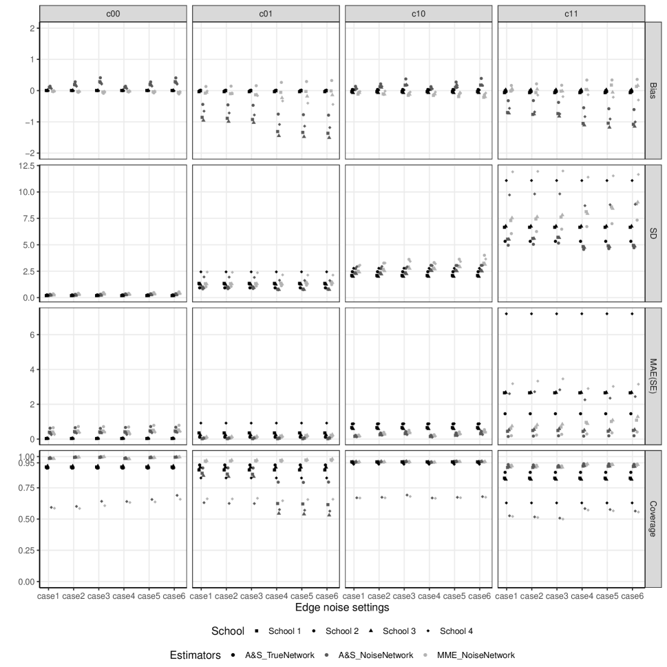
Figure 4.1: Biases, standard deviations, mean absolute errors of standard errors, and coverage rates of 95% confidence intervals in four schools.

From the plots, we see that method-of-moments estimators outperform Aronow and Samii estimators in noisy networks, and essentially perform the same on noisy networks as Aronow and Samii estimators do on noise-free networks (same zero biases with, at times, just slightly larger standard deviations). Aronow and Samii estimators in noisy networks underestimate $\bar{y}(c_{11})$ and $\bar{y}(c_{01})$ and overestimate $\bar{y}(c_{10})$ and $\bar{y}(c_{00})$. And the biases of Aronow and Samii estimators for $\bar{y}(c_{11})$ and $\bar{y}(c_{01})$ increase as $\alpha$ and $\beta$ increase, while the biases of Aronow and Samii estimators for $\bar{y}(c_{01})$ and $\bar{y}(c_{00})$ only depend on $\beta$. The biases of method-of-moments estimators are close to zero in all cases. In addition, standard deviations of the three types estimators are similar in all cases. The standard deviations of estimators in School 4 are larger than those in other schools because the network size in School 4 is relatively small.

In addition, the standard errors of method-of-moments estimators are close to the corresponding standard deviations expect for the exposure level $c_{11}$ in School 4. The network size in School 4 is small, so there is almost no individual in exposure level $c_{11}$. Thus, we are unable to impute missing counterfactuals accurately, which leads to inaccurate variance estimators. Furthermore, the variances of bias estimate are large because of the small network size in School 4. Therefore, we cannot obtain good bias estimators. The inaccurate bias and variance estimators in School 4 lead to relatively low coverage rates for method-of-moments estimators.

5 Discussion

Here we have quantified biases and variances of standard estimators in noisy networks and developed a general framework for estimation of true average causal effects in contexts wherein one has observations of noisy networks. Our approach requires knowledge or consistent estimates of the corresponding noise parameters, the latter which can be obtained with as few as three replicates of network observations. We employ method-of-moments techniques to derive estimators and establish their asymptotic unbiasedness, consistency, and normality. Simulations in British secondary schools contact networks demonstrate that substantial inferential accuracy by method-of-moments estimators is possible in networks of even modest size when nontrivial noise is present.

We have pursued a frequentist approach to the problem of uncertainty quantification for estimating average causal effects. If the replicates necessary for our approach are unavailable in a given setting, a Bayesian approach is a natural alternative. For example, posterior-predictive checks for goodness-of-fit based on examination of a handful of network summary measures is common practice (e.g., Bloem-Reddy and Orbanz, (2018)). Note, however, that the Bayesian approach requires careful modeling of the generative process underlying $G$ and typically does not distinguish between signal and noise components. Our analysis is conditional on $G$, and hence does not require that $G$ be modeled. It is effectively a ‘signal plus noise’ model, with the signal taken to be fixed but unknown. Related work has been done in the context of graphon modeling, with the goal of estimating network motif frequencies (e.g., Latouche and Robin, (2016)). However, again, one typically does not distinguish between signal and noise components in this setting. Additionally, we note that the problem of practical graphon estimation itself is still a developing area of research.

Our work here sets the stage for extensions to other potential outcome frameworks and exposure models. Here we sketch the key elements of one such extension. For example, consider the exposure mapping $f$ as following:

$$f(\bm{z},\bm{A}_{\cdot i})=\begin{cases}c_{11^{\prime}}\text{(Direct + $\geq$ $m_{i}$ Neighborhood Exposure)},&z_{i}I_{\{\bm{z}^{\top}\bm{A}_{\cdot i}>0\}}\geq m_{i},\\ c_{10^{\prime}}\text{(Direct + $<$ $m_{i}$ Neighborhood Exposure)},&z_{i}I_{\{\bm{z}^{\top}\bm{A}_{\cdot i}>0\}}<m_{i},\\ c_{01^{\prime}}\text{( $\geq m_{i}$ Neighborhood Exposure)},&(1-z_{i})I_{\{\bm{z}^{\top}\bm{A}_{\cdot i}>0\}}\geq m_{i},\\ c_{00^{\prime}}\text{( $<m_{i}$ Neighborhood Exposure)},&(1-z_{i})I_{\{\bm{z}^{\top}\bm{A}_{\cdot i}>0\}}<m_{i},\\ \end{cases}$$ (5.1)

where $m_{i}\geq 1$. When $m_{i}=1$, it reduces to (1.2). And if $m_{i}=k$, then the level $c_{11^{\prime}}$ is known as the absolute $k$-neighborhood exposure (Ugander et al., (2013)). When $m_{i}=qd_{i}$, $0\leq q\leq 1$, the level $c_{11^{\prime}}$ is called the fractional $q$-neighborhood exposure (Ugander et al., (2013)). The generalized four-level exposure model provides useful abstractions for the analysis of networked experiments. For example, infectious diseases (e.g., like COVID-19) are more likely to spread between people closely connected in a social network. And being in contact with more people with the disease means that, in theory, they are more likely to contract the disease.

As an illustration, suppose that treatment is assigned to the $N_{v}$ individuals in a network through Bernoulli random sampling, with probability $p$. The exposure probabilities for four levels can be found in supplementary material D. Next, we show orders of the exposure probabilities for nodes with varying degrees in Theorem 8. If $d_{i}=\Theta(1/p)$, upper bounds for four exposure probabilities do not depend on $m_{i}$. When $d_{i}=\omega(1/p)$, upper bounds for $p_{i}^{e}(c_{10^{\prime}})$ and $p_{i}^{e}(c_{00^{\prime}})$ increase as $m_{i}$ increases. And upper bounds for $p_{i}^{e}(c_{11^{\prime}})$ and $p_{i}^{e}(c_{01^{\prime}})$ decrease as $m_{i}$ increases if $d_{i}=o(1/p)$. See supplementary material D for the proof.

Theorem 8

Assume a generalized four-level exposure model and Bernoulli random assignment of treatment with $p=o(1)$. And for all $i$, $d_{i}\geq m_{i}$. Then, for all integers $m_{i}\geq 1$ and $m_{i}=\mathcal{O}(1)$, the orders of exposure probabilities are as follows.

	$p_{i}^{e}(c_{11^{\prime}})$	$p_{i}^{e}(c_{10^{\prime}})$	$p_{i}^{e}(c_{01^{\prime}})$	$p_{i}^{e}(c_{00^{\prime}})$
$d_{i}=\omega(1/p)$	$\mathcal{O}(p)$	$\mathcal{O}(p(d_{i}p)^{m_{i}-1}/e^{d_{i}p})$	$\mathcal{O}(1)$	$\mathcal{O}((d_{i}p)^{m_{i}-1}/e^{d_{i}p})$
$d_{i}=\Theta(1/p)$	$\mathcal{O}(p)$	$\mathcal{O}(p)$	$\mathcal{O}(1)$	$\mathcal{O}(1)$
$d_{i}=o(1/p)$	$\mathcal{O}(p(d_{i}p)^{m_{i}})$	$\mathcal{O}(p)$	$\mathcal{O}((d_{i}p)^{m_{i}})$	$\mathcal{O}(1)$

Then, we can construct regularity conditions for the average causal effect estimators to be consistent. Similarly, one can quantify biases and variances of standard estimators in noisy networks and develop a general framework for estimation of true average causal effects. These require additional work due to the complexities of formulas for exposure probabilities.

Our choice to work with independent network noise is both natural and motivated by convenience. A precise characterization of the noise dependency would be needed to extend our work, but is typically problem-specific and hence a topic for further investigation.

6 Supplementary Materials

Supplementary Materials for “Causal Inference under Network Interference with Noise”: Providing proofs of all propositions and theorems presented in the main paper.

Data and code accessibility: No primary data are used in this paper. Secondary data source is taken from Kucharski et al., (2018). These data and the code necessary to reproduce the results in this paper are available at https://github.com/KolaczykResearch/CausInfNoisyNet.

7 Acknowledgement

This work was supported in part by ARO award W911NF1810237. This work was also supported by the Air Force Research Laboratory and DARPA under agreement number FA8750-18-2-0066 and by a grant from MIT Lincoln Labs.

8 Appendix

In this appendix, we provide arguments for the consistency of contrast estimates in noise-free networks and regularity conditions in noisy networks.

8.1 Consistency of contrast estimates in noise-free networks

We first establish conditions for the estimator $\hat{\uptau}(c_{k},c_{l})$ to converge to $\uptau(c_{k},c_{l})$ as $N_{v}\rightarrow\infty$. We will show that, under two regularity conditions, $\hat{\uptau}(c_{k},c_{l})\xrightarrow{P}\uptau(c_{k},c_{l})$ as $N_{v}\rightarrow\infty$. Note that these conditions are similar to but slightly more general than the conditions in Aronow and Samii, (2017).

Condition 1

For all values $i$ and $c_{k}$, $|y_{i}(c_{k})|\leq c<\infty$, $p^{e}_{i}(c_{k})>0$ and $\sum_{i=1}^{N_{v}}1/p^{e}_{i}(c_{k})=o(N_{v}^{2})$, where $c$ is a constant.

We will also make an assumption about the amount of dependence among exposure conditions in the population. Let $p_{ij}^{e}(c_{k})=\sum_{\bm{z}}p_{\bm{z}}I_{\{f({\bm{z}},{\bm{x}}_{i})=c_{k}\}}I_{\{f({\bm{z}},{\bm{x}}_{j})=c_{k}\}}$.

Condition 2

For all values $c_{k}$, $\sum_{i=1}^{N_{v}}\sum_{j\neq i}^{N_{v}}|p^{e}_{ij}(c_{k})/(p^{e}_{i}(c_{k})p^{e}_{j}(c_{k}))-1|=o(N_{v}^{2})$.

Condition 2 implies that the amount of pairwise clustering in exposure conditions is limited in scope as $N_{v}$ grows. Condition 2 can be relaxed, though Condition 1 would likely need to be strengthened accordingly.

Proposition 1

Given Conditions 1 and 2, $\hat{\uptau}(c_{k},c_{l})\xrightarrow{P}\uptau(c_{k},c_{l})$ as $N_{v}\rightarrow\infty$.

Assuming the four-level exposure model in (1.2) and Bernoulli random assignment of treatment with probability $p$, we consider the consistency of the estimator $\hat{\uptau}(c_{k},c_{l})$ in two typical classes of networks: homogeneous and inhomogeneous.

Proposition 2 (Homogeneous)

Assume a four-level exposure model and Bernoulli random assignment of treatment with $p$. In the homogeneous network setting, under Assumption 4, $\hat{\uptau}(c_{k},c_{l})\xrightarrow{P}\uptau(c_{k},c_{l})$ as $N_{v}\rightarrow\infty$.

Proposition 3 (Inhomogeneous)

Assume a four-level exposure model and Bernoulli random assignment of treatment with $p$. In the inhomogeneous network setting, under Assumption 4, $\lambda=\Theta(p)$ and $\lambda>p$, we have $\hat{\uptau}(c_{k},c_{l})\xrightarrow{P}\uptau(c_{k},c_{l})$ as $N_{v}\rightarrow\infty$.

Proofs for Propositions 1 – 3 appear in the supplementary material A.

Note that, under Assumption 4, Condition 1 does not hold for levels $c_{10}$ and $c_{00}$ when the degrees follow a Pareto distribution with shape $\zeta>1$. This is because there are more high degree nodes, and $1/p_{i}^{e}(c_{10})$ and $1/p_{i}^{e}(c_{00})$ increase exponentially when the degree $d_{i}$ increases. See supplementary material E for the proof.

8.2 Standard estimators in noisy networks

Recall that under the Condition 1 and 2, $\hat{\uptau}(c_{k},c_{l})\xrightarrow{P}\uptau(c_{k},c_{l})$ as $N_{v}\rightarrow\infty$. By making assumptions on underlying rates of error $\alpha$ and $\beta$, we will show that similar regularity conditions hold for noisy homogeneous and inhomogeneous networks. These conditions will then be used in our characterization of bias and variance in Sections 2.2 and 2.3. Define $\tilde{p}_{ij}^{e}(c_{k})=\sum_{\bm{z}}p_{\bm{z}}I_{\{f({\bm{z}},\tilde{\bm{X}}_{i})=c_{k}\}}I_{\{f({\bm{z}},\tilde{\bm{X}}_{j})=c_{k}\}}$.

Proposition 4 (Homogeneous)

Assume a four-level exposure model and Bernoulli random assignment of treatment with $p$. In the homogeneous network setting, under Assumptions 1 - 5, for all values $i$ and $c_{k}$, $\mathbb{P}(\tilde{p}^{e}_{i}(c_{k})>0)\rightarrow 1$, $\mathbb{E}[\sum_{i=1}^{N_{v}}I_{\{\tilde{p}^{e}_{i}(c_{k})>0\}}/\tilde{p}^{e}_{i}(c_{k})]=o(N_{v}^{2})$, and $\mathbb{E}[\sum_{i=1}^{N_{v}}\sum_{j\neq i}^{N_{v}}I_{\{\tilde{p}^{e}_{i}(c_{k})>0\}}I_{\{\tilde{p}^{e}_{j}(c_{k})>0\}}|\tilde{p}^{e}_{ij}(c_{k})/(\tilde{p}^{e}_{i}(c_{k})\tilde{p}^{e}_{j}(c_{k}))-1|]=o(N_{v}^{2})$.

Proposition 5 (Inhomogeneous)

Assume a four-level exposure model and Bernoulli random assignment of treatment with $p$. In the inhomogeneous network setting, under Assumptions 1- 5, $\lambda=\Theta(p)$ and $\lambda>p$, the statements in Proposition 4 hold for all values $i$ and $c_{k}$.

See supplementary material B for proofs of Propositions 4 and 5.

References

- Abadie and Imbens, (2006) Abadie, A. and Imbens, G. W. (2006). Large sample properties of matching estimators for average treatment effects. econometrica, 74(1):235–267.
- Ahmed et al., (2014) Ahmed, N. K., Neville, J., and Kompella, R. (2014). Network sampling: From static to streaming graphs. ACM Transactions on Knowledge Discovery from Data (TKDD), 8(2):7.
- Alvarez and Levin, (2014) Alvarez, R. M. and Levin, I. (2014). Uncertain neighbors: Bayesian propensity score matching for causal inference. Technical report, Technical report, California Institute of Technology, University of Georgia.
- Amaral et al., (2000) Amaral, L. A. N., Scala, A., Barthelemy, M., and Stanley, H. E. (2000). Classes of small-world networks. Proceedings of the national academy of sciences, 97(21):11149–11152.
- An, (2010) An, W. (2010). 4. bayesian propensity score estimators: Incorporating uncertainties in propensity scores into causal inference. Sociological Methodology, 40(1):151–189.
- Aronow and Samii, (2017) Aronow, P. M. and Samii, C. (2017). Estimating average causal effects under general interference, with application to a social network experiment. The Annals of Applied Statistics, 11(4):1912–1947.
- Athey et al., (2018) Athey, S., Eckles, D., and Imbens, G. W. (2018). Exact p-values for network interference. Journal of the American Statistical Association, 113(521):230–240.
- Balachandran et al., (2017) Balachandran, P., Kolaczyk, E. D., and Viles, W. D. (2017). On the propagation of low-rate measurement error to subgraph counts in large networks. The Journal of Machine Learning Research, 18(1):2025–2057.
- Bhattacharya et al., (2019) Bhattacharya, R., Malinsky, D., and Shpitser, I. (2019). Causal inference under interference and network uncertainty. In Uncertainty in artificial intelligence: proceedings of the… conference. Conference on Uncertainty in Artificial Intelligence, volume 2019. NIH Public Access.
- Bloem-Reddy and Orbanz, (2018) Bloem-Reddy, B. and Orbanz, P. (2018). Random-walk models of network formation and sequential monte carlo methods for graphs. Journal of the Royal Statistical Society: Series B (Statistical Methodology), 80(5):871–898.
- Chang et al., (2020) Chang, J., Kolaczyk, E. D., and Yao, Q. (2020). Estimation of subgraph densities in noisy networks. Journal of the American Statistical Association, pages 1–14.
- Chatterjee et al., (2015) Chatterjee, S. et al. (2015). Matrix estimation by universal singular value thresholding. The Annals of Statistics, 43(1):177–214.
- Clauset et al., (2009) Clauset, A., Shalizi, C. R., and Newman, M. E. (2009). Power-law distributions in empirical data. SIAM review, 51(4):661–703.
- Cox and Cox, (1958) Cox, D. R. and Cox, D. R. (1958). Planning of experiments, volume 20. Wiley New York.
- Grizzle, (1965) Grizzle, J. E. (1965). The two-period change-over design and its use in clinical trials. Biometrics, pages 467–480.
- Horvitz and Thompson, (1952) Horvitz, D. G. and Thompson, D. J. (1952). A generalization of sampling without replacement from a finite universe. Journal of the American statistical Association, 47(260):663–685.
- Hudgens and Halloran, (2008) Hudgens, M. G. and Halloran, M. E. (2008). Toward causal inference with interference. Journal of the American Statistical Association, 103(482):832–842.
- Imbens and Menzel, (2021) Imbens, G. and Menzel, K. (2021). A causal bootstrap. The Annals of Statistics, 49(3):1460 – 1488.
- Jiang et al., (2011) Jiang, X., Gold, D., and Kolaczyk, E. D. (2011). Network-based auto-probit modeling for protein function prediction. Biometrics, 67(3):958–966.
- Jiang and Kolaczyk, (2012) Jiang, X. and Kolaczyk, E. D. (2012). A latent eigenprobit model with link uncertainty for prediction of protein–protein interactions. Statistics in Biosciences, 4(1):84–104.
- Kempton and Lockwood, (1984) Kempton, R. and Lockwood, G. (1984). Inter-plot competition in variety trials of field beans (vicia faba l.). The Journal of Agricultural Science, 103(2):293–302.
- Kolaczyk, (2009) Kolaczyk, E. D. (2009). Statistical Analysis of Network Data. Springer.
- Kucharski et al., (2018) Kucharski, A. J., Wenham, C., Brownlee, P., Racon, L., Widmer, N., Eames, K. T., and Conlan, A. J. (2018). Structure and consistency of self-reported social contact networks in british secondary schools. PloS one, 13(7):e0200090.
- Latouche and Robin, (2016) Latouche, P. and Robin, S. (2016). Variational bayes model averaging for graphon functions and motif frequencies inference in w-graph models. Statistics and Computing, 26(6):1173–1185.
- Le and Li, (2020) Le, C. M. and Li, T. (2020). Linear regression and its inference on noisy network-linked data. arXiv preprint arXiv:2007.00803.
- Manski, (2013) Manski, C. F. (2013). Identification of treatment response with social interactions. The Econometrics Journal, 16(1):S1–S23.
- Neyman, (1923) Neyman, J. (1923). Sur les applications de la theorie des probabilites aux experiences agricoles: essai des principes (masters thesis); justification of applications of the calculus of probabilities to the solutions of certain questions in agricultural experimentation. excerpts english translation (reprinted). Stat Sci, 5:463–472.
- Priebe et al., (2015) Priebe, C. E., Sussman, D. L., Tang, M., and Vogelstein, J. T. (2015). Statistical inference on errorfully observed graphs. Journal of Computational and Graphical Statistics, 24(4):930–953.
- Rosenbaum, (1999) Rosenbaum, P. R. (1999). Reduced sensitivity to hidden bias at upper quantiles in observational studies with dilated treatment effects. Biometrics, 55(2):560–564.
- Ross, (1916) Ross, R. (1916). An application of the theory of probabilities to the study of a priori pathometry.–part i. Proceedings of the Royal Society of London. Series A, Containing papers of a mathematical and physical character, 92(638):204–230.
- Rubin, (1990) Rubin, D. B. (1990). Formal mode of statistical inference for causal effects. Journal of statistical planning and inference, 25(3):279–292.
- Schafer and Kang, (2008) Schafer, J. L. and Kang, J. (2008). Average causal effects from nonrandomized studies: a practical guide and simulated example. Psychological methods, 13(4):279.
- Smieszek et al., (2012) Smieszek, T., Burri, E. U., Scherzinger, R., and Scholz, R. W. (2012). Collecting close-contact social mixing data with contact diaries: reporting errors and biases. Epidemiology & infection, 140(4):744–752.
- Sussman and Airoldi, (2017) Sussman, D. L. and Airoldi, E. M. (2017). Elements of estimation theory for causal effects in the presence of network interference. arXiv preprint arXiv:1702.03578.
- Toulis and Kao, (2013) Toulis, P. and Kao, E. (2013). Estimation of causal peer influence effects. In International conference on machine learning, pages 1489–1497.
- Ugander et al., (2013) Ugander, J., Karrer, B., Backstrom, L., and Kleinberg, J. (2013). Graph cluster randomization: Network exposure to multiple universes. In Proceedings of the 19th ACM SIGKDD international conference on Knowledge discovery and data mining, pages 329–337.
- Young et al., (2020) Young, J.-G., Cantwell, G. T., and Newman, M. (2020). Robust bayesian inference of network structure from unreliable data. arXiv preprint arXiv:2008.03334.