An end-to-end Optical Character Recognition approach for ultra-low-resolution printed text images

Abstract

Some historical and more recent printed documents have been scanned or stored at very low resolutions, such as 60 dpi. Though such scans are relatively easy for humans to read, they still present significant challenges for optical character recognition (OCR) systems. The current state-of-the art is to use super-resolution to reconstruct an approximation of the original high-resolution image and to feed this into a standard OCR system. Our novel end-to-end method bypasses the super-resolution step and produces better OCR results. This approach is inspired from our understanding of the human visual system, and builds on established neural networks for performing OCR.

Our experiments have shown that it is possible to perform OCR on 60 dpi scanned images of English text, which is a significantly lower resolution than the state-of-the-art, and we achieved a mean character level accuracy (CLA) of 99.7% and word level accuracy (WLA) of 98.9% across a set of about 1000 pages of 60 dpi text in a wide range of fonts. For 75 dpi images, the mean CLA was 99.9% and the mean WLA was 99.4% on the same sample of texts. We make our code and data (including a set of low-resolution images with their ground truths) publicly available as a benchmark for future work in this field.

I Introduction

The current generation of optical character recognition (OCR) software is designed for recognising printed text at 300 dpi. For lower resolutions down to about 150 dpi, the image can be enlarged to 300 dpi prior to performing the OCR step using bicubic interpolation, and the results are still excellent. (For example, when testing this on our scanned text dataset, described in section IV-A, we found that on average, reducing the 300 dpi images by a factor of 2 and then enlarging them back to 300 dpi using bicubic interpolation resulted in slightly better recognition results when using the standard Tesseract OCR software. An analysis of this behaviour is beyond the scope of this paper.)

Document images at resolutions less than about 150 dpi offer much greater challenges, as much less information is present in the image. (See, for example [1], [2] and the other sources discussed in section II. We give illustrative numerical results for our dataset in section IV below.) This might happen if images are stored at a very low resolution for space purposes, or if photographs of scenes containing text have been captured from a distance so the text within them is very small. In this work, we have focused our attention on scanned documents, but there are clear potential extensions of our technique to other use cases.

It is astonishing that humans are able to read such low-resolution images with relative ease when printed at this low resolution. However, things are very different when they are enlarged. For example, figure 1 shows a word in a 60 dpi document, enlarged so that the individual pixels are visible. It is difficult to visually determine what the word is and even where the character boundaries are. In spite of this, when the image is held at a distance (or made smaller), the characters become quite distinct and reasonably easy to read. In contrast to this, figure 2 shows a different word at 300 dpi, enlarged to the same size; this is easily readable from both nearby and from a distance. A standard OCR system trained to recognise 300 dpi images of 10 point text will have significant difficulty with figure 1, even if it is enlarged to 300 dpi using bicubic interpolation (as in Figure 4).

Figure 1: A word from a 60 dpi scan, enlarged so that the individual pixels are visible.

Figure 2: A simulated word from a 300 dpi scan, enlarged so that the individual pixels are visible.

In this work, we have taken a novel approach to this problem, building on certain existing ideas, but introducing a new human-vision-inspired technique. Our main contributions are:

• Performing OCR on 60 dpi scanned printed text, and achieving outstanding character and word recognition rates; OCR on such ultra-low-resolution images has not been previously reported.

• Performing OCR on 75 dpi images, and achieving character and word recognition rates significantly in excess of previously reported results for some fonts.

• Demonstrating how sensitive OCR of low-resolution images can be to the font used, suggesting that it might be very hard to develop an OCR system which works well on all low-resolution images.

We note that we cannot directly compare our results with those appearing in the literature, as there is no standard benchmark dataset for this problem and none of the software developed is publicly available. We are therefore limited to quoting the results appearing in those papers. Also, as we note later, low-resolution OCR is very sensitive to the font used and to the precise nature of the images, making it even harder to directly compare our results. To help remedy this situation, we have prepared a test dataset that could be used for future benchmarking, as described in section IV-A below.

The rest of the paper is structured as follows. In section II, we briefly survey related work. In section III, we discuss one aspect of human vision and how it is related to our problem, and then explain our approach in detail. We present and analyse our results in section IV. A summary of our algorithm is displayed in figures 5 to 7.

II Related work

One early approach for performing OCR on low-resolution text images was presented in [3] and [4] in the context of images captured by low-resolution cameras. The issues they faced were primarily around blurriness; the image resolution was on the effective order of 150–200 dpi. They used a neural network to recognize individual characters, followed by a separate word recognition phase.

More recently, there has been renewed effort to address low-resolution images in the 75–100 dpi range. Several authors consider using multiple thresholds for binarisation of the images and then using an ensemble method on the OCR output produced from each (such as [2], [5] and [6]); these approaches are suitable for OCR systems that work by initially thresholding a greyscale image to produce a binary image before performing segmentation and feature extraction.

A second popular approach has been to use super-resolution (for example, [7], [1], [8], [9] and [10]). This approach was also perhaps partially spurred on by the ICDAR 2015 Competition on Text Image Super-Resolution ([11], [12] and [13]), which aimed to recognise text from frames extracted from video streams. The task was to reconstruct a high-resolution image from a low resolution one, and to then use that to perform OCR. (It is important to note that super-resolution is not simply upscaling using bicubic interpolation or similar, but rather an attempt to match the original image. The quality of a super-resolution reconstruction is typically measured using a metric such as PSNR, comparing the reconstruction with the ground truth high-resolution image.) There has been considerable success with this method. For example, Pandey et al. [9] reported OCR results for 75 dpi English text as 75.1% CLA (character level accuracy) and 48% WLA (word level accuracy). They achieved significantly better results on 75 dpi Tamil (90.8% CLA and 54.3% WLA) and Kannada (95.16% WLA and 70.80% WLA). A more powerful super-resolution technique used by Lat and Jawahar [10], and their quoted results are the best we are aware of. Their OCR results depended upon the OCR tool being used: the commercial ABBYY achieved 97.88% CLA and 95.20% WLA on their swd dataset, while the open source Tesseract version 3.x achieved 85.96% CLA and 89.70% WLA; ABBYY also achieved 99.65% CLA and 98.90% WLA on their end dataset.

There are some issues with Lat and Jawahar’s [10] methodology, which makes it difficult to directly compare their results with other quoted results. Though the precise texts chosen for their end test set are different from the training texts, the generation process was presumably the same, and so this only shows (the still impressive result) that their GAN super-resolution scheme can very accurately reconstruct high-resolution images from low-resolution images if they are of a very similar nature to the training images. However, with real-life scanners, different scanners may produce different behaviours from simulations, and so it is necessary to test any proposed system with real scanners. Also, for their swd dataset, it seems from their Figure 7 that these images are captured at closer to 100 dpi than 75 dpi, so it is unsurprising that they give relatively good results.

None of these researchers reported attempting OCR with 60 dpi images: whilst even 50 dpi images were improved using super-resolution (for example, Pandey and Ramakrishnan [9] report an average PSNR of 16.89 for super-resolved 50 dpi images and 19.36 for 75 dpi images), the OCR systems are relatively poor at extracting text from such noisy images, and so the accuracy rate would be even lower for super-resolved 60 dpi images. We also note at this point that 60 dpi images contain only about 60% as many pixels as the corresponding 75 dpi images, making the task significantly harder.

Super-resolving the image is of interest to humans, who would like to see a higher-resolution image, but our primary goal here is to extract text from the image. Furthermore, as is clear from figure 1 above, it can be challenging to even determine whether such a low-resolution image is even of a sans serif or a serif font. A super-resolved 300 dpi image starting from this would be quite likely to hallucinate much of the detail, and even if it did perform this step reasonably well, a standard OCR system might well struggle with the resulting image.

One possible approach is to create an end-to-end loss function, where a single neural network performs super-resolution followed by OCR, and the loss function is determined by the OCR accuracy. Another approach, which is close to the one we have taken in this paper, is to skip the super-resolution step entirely, and to perform OCR directly on the original image. Such an approach was, to the best of our knowledge, first taken by Wang and Singh [14], who designed a RNN-LSTM neural network to replace Tesseract 3.02’s feature-based character recognition system, and trained a network on a collection of domain-specific text lines generated at 72 dpi, 100 dpi, 150 dpi, 200 dpi and 300 dpi. This RNN-LSTM network had an input height of 32 pixels, so they scaled the images of text lines, both during training and recognition, to this height using spline interpolation. (We emphasise that this scaling is not an attempt to perform super-resolution.) Their quoted result for 72 dpi images is a CLA of 91.95%. Since then, Tesseract 4.0.0 has been released, which uses a similar neural network for recognition, but is only trained on 300 dpi images.

III Our human-vision inspired approach

III-A Human vision

Figure 3: Figure 1, enlarged to 300 dpi with nearest-neighbour interpolation and then filtered with a low-pass spatial Gaussian filter.

Figure 4: Figure 1, enlarged to 300 dpi using bicubic interpolation.

It is remarkable that most people are able to read the word in figure 1 when they hold it at a distance. The cause of this was researched in detail by Majaj et al. [15]. At a far distance (or at a small size, which is effectively the same), our visual system primarily processes the low-frequency information (the gross shape of the letters), whereas at a near distance (or large size), we process higher-frequency information (the edges of the letters). For a low-resolution text image such as this, the high-frequency (edge) information is mostly noise, so it is impossible to identify letters from this, whereas the low-frequency information still contains approximately enough information to identify the letters. (The concept that different frequencies are perceived at different distances has also been successfully developed by Oliva et al [16] to create hybrid images, for example making a piece of text visible from nearby but invisible at a distance; a well-known example of this phenomenon is the Marilyn Monroe and Albert Einstein hybrid.)

One way we could therefore hope to improve the performance of an OCR system on these low-resolution images is to upscale them to 300 dpi (the resolution on which the OCR systems are trained) using nearest-neighbour interpolation and then blur the images using a small Gaussian filter. This has the effect of reducing the high-frequency components and making the edges less distinct. A similar effect results from using bilinear or bicubic interpolation. As a result, the word becomes easier to read; results of doing this to the word in figure 1 are shown in figure 3 and figure 4.

III-B Current OCR systems

Figure 5: A schematic illustration of our low-resolution OCR ensembling approach: (1) a low-resolution image is upscaled and blurred in multiple different ways; (2) each upscaled image is recognised using an LSTM trained for that type of upscaling, the results of which include confidences for each word; (3) the results are merged to produce the best option for each word, taking a dictionary into account. An example of the merging algorithm in action is shown in figure 7.

Figure 6: A schematic illustration of our modified version of Tesseract for low-resolution images, where the green arrows indicate new steps and the red arrow indicates a replaced step: (1) the original low-resolution image is upscaled and blurred to make a 300 dpi image; (2) the page is segmented and the text lines extracted; (3) (original Tesseract only) each text line is scaled to 36 pixels high; (4) each 36-pixel high scaled text line is produced using upscaling and blurring directly from the original image; (5) the text line is passed to an LSTM network with a CTC; (6) textual output and confidences for each word are produced.

Figure 7: Merging different results, the final step of the pipeline in figure 5. (a) The words identified when performing OCR using one type of upscaling; the colours are a visual representation of the confidence level, and the textual results are shown below it (with a number such as [16] meaning 16% confidence). (b) The results using a different upscaling. (c) Merger of (a) and (b) using our algorithm. The small bands of colour above and below the images are from adjacent lines of text. Note that the bounding boxes of the identified words differ significantly between the two images.

State-of-the-art OCR systems now use trained bidirectional-LSTM neural networks to perform the character recognition step. Probably the best-known open source OCR system available today is Tesseract [17], which has used such a network since version 4.0.0 (see, for example, [18], section 6 of [19] and [20]). In brief, Tesseract first segments the page into areas of text, which are further subdivided into paragraphs and then lines. Each line is passed into the trained network, which uses a final softmax layer attached to a CTC (connectionist temporal classifier) ([21], [19]) to determine the most likely sequence of letters and spaces; these are then further processed to produce a sequence of words. Each letter and each word also carries with it a confidence score, based on the output of the classifier, and Tesseract can be instructed to output this information.

III-C Modifying Tesseract

Tesseract is designed to be trainable, and so we would like to train it to recognise upscaled images. A small issue arises in training it directly on upscaled images, so we slightly modified the program to handle them, as we now explain. A sketch of Tesseract’s pipeline (version 4.1.1 of the software) is shown in figure 6, together with our modifications. We choose an upscaling method and apply it consistently for training and recognition. The upscalings that we used in this work were: upscaling using nearest neighbour interpolation followed by a spatial Gaussian filter with standard deviation 0, 0.5, 1, 1.5 or 2 pixels in the 300 dpi upscaled image; bilinear interpolation (with no filtering), and bicubic interpolation (also with no filtering). (In our implementation, we have referred to nearest neighbour interpolation as box interpolation; for upscaling, these are equivalent.) Tesseract is given the low-resolution image and upscales it to 300 dpi in the manner specified. It then performs its page segmentation as normal, and extracts a text line. At this point, Tesseract would scale the text line to make it the correct height for the trained LSTM network (which happens to be 36 pixels), using linear interpolation and unsharp masking. Since our image has already been upscaled once, this would potentially lead to the loss of information, so we instead produce the required region by upscaling the original image. (This is why we chose to modify the software rather than directly training on upscaled images.) During training, we use this image to train the LSTM network for this type of upscaling, and during recognition, we use that specifically-trained network.

For the training phase, we used transfer learning, beginning with the Tesseract ‘best’ English network (available from the Tesseract repository). We generated lines of low-resolution text in a variety of fonts at a variety of font sizes (from 9pt to 12pt), adding small amounts of Gaussian noise to the results, and also randomly rotating half of them by a small angle (normally distributed with mean $0^{\circ}$ and standard deviation $0.5^{\circ}$) to mimic the effect of scans being slightly askew. If we were training for a specific type of document, it would make sense to train using lines of text from that genre of document, as the LSTM will learn patterns of languages. (This is what is done in [14].) However, we have chosen here to train our system for a wide variety of texts, so we have used the Tesseract training texts, which consists of about 170 000 lines of random English ‘words’ gleaned from a variety of sources. It is not clear how many lines of text it is best to train on to avoid over-fitting, so for our experiments, we trained on 10% of them and also on 100% of them; we compare the results below. For each of these, we randomly chose 90% of the lines to be used for training and 10% for validation (‘evaluation’ in Tesseract’s terminology). For the training on the entire 170 000 text lines, we performed this in 10 separate steps to allow the possibility of evaluating the performance on different sizes of training data. We separately trained Tesseract for 60 dpi images and for 75 dpi images.

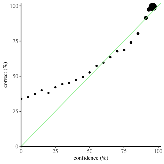
Figure 8: The proportion of words in 20 000 random lines of text (from the Tesseract training texts) that are correctly recognised, plotted against the confidence that Tesseract has in the word. This is the average across all seven upscaling methods produced for 60 dpi images. The sizes of the dots are proportional to the frequency of words with this confidence, and words with confidence scores less than 95 are binned together.

III-D An ensemble method

Initial small experiments showed that there was little consistency about which type of upscaling gave the best recognition results across texts; furthermore, this varied on a word-by-word basis. We therefore decided to use an ensemble method, combining the Tesseract outputs from different upscalings to give the best possible output, at the cost of running time. As noted earlier, ensembling approaches to OCR have been explored by a number of researchers. However, we have more information than they did: Tesseract can be instructed to provide a confidence score and bounding box for each word. (The confidence score is determined from the final softmax layer and the CTC in a somewhat complex way whose details do not concern us here.) We therefore wish to take account of the confidence of the different outputs, not just their counts. There are two key complexities to address here:

1. Determining when two words output by Tesseract represent the same piece of text; as can be seen in Figure 7, the bounding boxes determined for the same word in different recognition passes can be very different, and one word can even appear as two words or be entirely missing in a different pass.

2. Deciding how to perform a majority vote taking confidences into account.

There are several difficulties in implementing point (a) above. For example, if a word appears at a particular location in one output but no word appears at that location in another, what should we do? If we do decide to use that word, where in the text should it be inserted? (We must recall that our primary goal is to recognise the original text, and the order of words is a critical part of this, not just their location on the page.) This is further compounded when Tesseract’s page segmentation algorithm splits up the page in different ways with different upscalings. Several attempts to address this were unsuccessful, and for this reason, we opted for a simpler approach which works well most of the time. We designate one output as the master output, and compare all other outputs to that. For every word in the master output, we consider all the words in the corresponding locations in the other outputs whose bounding box is approximately the same as the master output’s bounding box, and ensemble the words so identified. This means that the number of words being ensembled at a particular point may be fewer than the number of Tesseract outputs; in the example shown in Figure 7, taking output (a) as the master output, the final word ‘Payment." ’ does not match anything in output (b), and the words ‘Pa’ and ‘l" ’ in output (b) are ignored. Finally, the choice of the master output was determined by the performance of the modified Tesseract on a large sample of lines of text drawn from the training set. It turned out that for 60 dpi, nearest neighbour plus a Gaussian filter with a standard deviation of 1 pixel was best, while bicubic interpolation was best for 75 dpi; these were therefore used as the respective master outputs.

For point (b), a further complication is the non-linearity of the confidences in relation to the accuracy when working with low-resolution images. Figure 8 shows the case for a large set of 60 dpi images: while the word confidence scores for 300 dpi images turn out to be a fairly good estimate of the probability of the word being correctly identified, this is not the case for 60 dpi images. There is also a lot of variation in this between different fonts (not shown here). We therefore work with a modified confidence score, which is a simple piecewise linear function giving a very rough approximation to this data:

$$c_{\text{mod}}=\begin{cases}0.5c+30&\text{if $c<80$}\\ 1.7c-65&\text{if $c\geq 80$}\end{cases}$$

(Though a confidence of 100 would give a modified confidence of over 100, Tesseract appears to never give a confidence score greater than 97.) A similar function is used for 75 dpi images based on the equivalent of Figure 8.

We now wish to perform a majority vote on each word, taking the modified confidence scores into account. There does not seem to be a principled way to do this, as we do not know what probability each network would give to other possible outputs. So we resort to the following: let the output words under consideration be $w^{(1)}$, …, $w^{(n)}$ with respective modified confidences $c_{\text{mod}}^{(1)}$, …, $c_{\text{mod}}^{(n)}$, and let $W$ be the set of distinct output words. Then we define the best output word to be

$$w_{\text{best}}=\operatorname*{arg\,max}_{w\in W}\frac{\sum_{\{i:w^{(i)}=w\}}c_{\text{mod}}^{(i)}}{\sqrt{|\{i:w^{(i)}=w\}|}}$$

This is somewhere between the sum of all modified confidences for a given possible output word and their mean, so that a repeated output with modified confidences of 40 and 41 do not override a single output with modified confidence of 80. Prior to doing this, we also reduce the modified confidence of outputs that are not dictionary words (after removing any punctuation) by 30; this gives some extra weight to dictionary words. The choice of 30 was experimentally determined as being a reasonable value on a small dataset, but slightly better results might be obtained by using a different penalty. We then replace the master output word with the ensemble output to produce the final output.

IV Results and discussion

IV-A Test data preparation

We tested our method on a large set of scanned images, none of which had been used in the training or algorithm development process. Furthermore, the training process generated images by simulation, while the test data was produced using a real scanner. To prepare the images, we chose 11 different texts: ten were taken from a variety of books in the Project Gutenberg [22] collection, including fiction, non-fiction and poetry, while one was taken from a recent U.S. Supreme Court opinion. (Details of the texts used are included in the public dataset we have made available.) Five pages of text were extracted from the start of each of these, totalling 124 961 characters and 25 656 words. Each page of text was typeset in 18 different fonts (so identical text appeared on each corresponding page). These fonts included: serif and sans serif fonts; monospaced and variable width fonts, and fonts which had been trained on and fonts which had not been used for training. The font sizes were all 10 pt or 11 pt, with the font size chosen so that the corresponding pages would each have about the same area of paper covered with text. The fonts used are listed in Table I. The resulting 990 pages were then printed at 600 dpi and scanned at 300 dpi. These scans were then down-sampled to 60 dpi and 75 dpi using box interpolation (which takes the average value of each $5\times 5$ or $4\times 4$ box of pixels respectively).

This variety allowed us to both test the effectiveness of our algorithm and to independently assess its performance on different types of text and on different fonts.

Font	Size	Serif	Mono	Train	Test
Arial	11 pt	no	no	yes	yes
Avenir	11 pt	no	no	yes	no
Baskerville	11 pt	yes	no	yes	yes
Bookman Old Style	11 pt	yes	no	no	yes
Calibri	11 pt	no	no	yes	yes
Cambria	11 pt	yes	no	no	yes
Century Gothic	10 pt	no	no	no	yes
Chalkboard	11 pt	no	no	yes	no
Comic Sans	10 pt	no	no	yes	yes
Courier New	10 pt	yes	yes	yes	yes
FrankRuehlCLM	11 pt	yes	no	yes	no
Franklin Gothic Book	11 pt	no	no	yes	yes
Futura	11 pt	no	no	yes	no
Garamond	11 pt	yes	no	no	yes
Gill Sans	11 pt	no	no	yes	yes
Helvetica	11 pt	no	no	yes	yes
Lucida Console	11 pt	no	yes	yes	no
Lucida Sans	10 pt	no	no	yes	yes
Menlo	10 pt	no	yes	yes	yes
Optima	11 pt	no	no	no	yes
Palatino	11 pt	yes	no	yes	yes
Tahoma	11 pt	no	no	yes	no
Trebuchet	11 pt	no	no	yes	no
Times New Roman	11 pt	yes	no	yes	yes
Verdana	10 pt	no	no	yes	yes

TABLE I: Fonts used for training and testing

The character level accuracy (CLA) and word level accuracy (WLA) are calculated by finding the Levenshtein distance $d$ between our algorithm’s output and the ground truth; the percentage accuracy is then calculated as $(1-\frac{d}{L})\times 100\%$, where $L$ is the number of characters or words in the ground truth. (For the CLA, we first collapse all sequences of white space into a single space character.)

One particular difficulty that quickly became apparent in initial experiments is that it is almost impossible to identify the type of quote marks used at these low resolutions; an open quote mark (‘), a straight quote mark (') and a close quote mark (’) all appear almost identical at 60 dpi. So in calculating the CLA and WLA, a decision was made to treat all three quote marks as equivalent (and similarly for double quotes and for dashes/hyphens).

IV-B Numerical results

	60 dpi plain		60 dpi lores		75 dpi plain		75 dpi lores		300 dpi
Font	CLA	WLA	CLA	WLA	CLA	WLA	CLA	WLA	CLA	WLA
Arial	99.4%	97.0%	99.8%	99.2%	99.8%	99.0%	99.9%	99.3%	99.9%	99.2%
Baskerville	99.1%	96.3%	99.6%	99.0%	99.8%	98.8%	99.8%	99.4%	99.9%	99.5%
Bookman Old Style	99.7%	98.3%	99.9%	99.7%	99.9%	99.5%	100.0%	99.8%	99.9%	99.6%
Calibri	99.4%	96.8%	99.8%	99.2%	99.8%	98.8%	99.9%	99.4%	99.9%	99.1%
Cambria	99.6%	97.8%	99.8%	99.0%	99.9%	99.1%	99.9%	99.7%	99.9%	99.4%
Century Gothic	96.6%	84.9%	99.2%	96.1%	99.2%	95.7%	99.7%	98.7%	99.7%	98.5%
Comic Sans	99.1%	95.1%	99.9%	99.4%	99.7%	98.3%	99.9%	99.6%	99.9%	99.3%
Courier New	98.9%	94.7%	99.8%	99.3%	99.7%	98.5%	99.9%	99.6%	99.9%	99.3%
Franklin Gothic Book	99.1%	95.6%	99.8%	99.2%	99.7%	98.5%	99.9%	99.3%	99.9%	99.2%
Garamond	97.1%	91.2%	98.8%	97.6%	99.7%	98.6%	99.7%	99.2%	99.9%	99.3%
Gill Sans	99.0%	95.4%	99.7%	98.9%	99.8%	98.7%	99.8%	99.2%	99.9%	99.2%
Helvetica	99.1%	96.1%	99.8%	99.1%	99.8%	98.6%	99.8%	99.2%	99.8%	98.9%
Lucida Sans	99.5%	97.5%	99.8%	99.2%	99.8%	98.7%	99.9%	99.3%	99.9%	99.1%
Menlo	99.5%	97.3%	99.9%	99.6%	99.9%	99.3%	99.9%	99.7%	99.9%	99.6%
Optima	99.6%	97.9%	99.9%	99.3%	99.8%	99.0%	99.9%	99.3%	99.9%	99.3%
Palatino	99.0%	97.8%	98.5%	98.0%	99.8%	99.3%	99.7%	99.3%	100.0%	99.7%
Times New Roman	99.5%	97.4%	99.8%	99.4%	99.8%	99.2%	99.9%	99.7%	100.0%	99.7%
Verdana	99.5%	97.4%	99.9%	99.6%	99.9%	99.4%	99.9%	99.7%	100.0%	99.7%

TABLE II: The average results on each font: the ‘plain’ results are with standard Tesseract on images upscaled with bicubic interpolation, while the ‘lores’ results are those obtained using our system. The final two columns give the results for plain Tesseract on the original 300 dpi images.

We present results for the 18 fonts tested in Table II, averaged across all 55 pages printed in that font. The results are shown for the networks trained on 100% of the Tesseract training lines; the results when the networks were trained on only 10% of the lines are very slightly worse. The table also shows the performance of plain Tesseract on the images when they have been upscaled to 300 dpi using bicubic interpolation. Our results show a significant improvement for 60 dpi images and a good improvement for 75 dpi images (for 60 dpi, the overall character error rate dropped by about 64% and the word error rate by about 73%; for 75 dpi, the corresponding figures are 35% and 51%). The only font which performs noticeably worse with our system is Palatino, and there is no clear reason for this.

We note at this point that even for 60 dpi images, these results are significantly better than the previous state-of-the-art’s quoted performance on 75 dpi images, and that the performance on both 60 dpi and 75 dpi images is close to that of plain Tesseract on 300 dpi images; for some fonts, our method even does slightly better on the 60 dpi images than plain Tesseract on the corresponding 300 dpi images!

Inspired by this, we also considered what would happen if we started with the 300 dpi scans and used our ensemble technique by taking the plain Tesseract run as the master output, and the results of downsampling the image to 75 dpi and using our modified Tesseract to produce the other outputs. Preliminary results indicate that the mean WLA improves somewhat, but the CLA declines. This is an area for further study.

We next look at the impact of different texts on the performance of this system. We use Cambria to illustrate this, as its performance is approximately in the middle of the fonts tested and it was not used during the training. Furthermore, we use the error rate (100% minus the accuracy rate) to make it easier to read the figures.

	60 dpi		75 dpi
Font	C err	W err	C err	W err
Around the World	0.07%	0.35%	0.01%	0.08%
Best Poetry	0.33%	1.45%	0.20%	0.77%
David Copperfield	0.41%	1.84%	0.15%	0.82%
Engineering	0.06%	0.33%	0.01%	0.04%
English Church	0.11%	0.48%	0.01%	0.03%
Fire Prevention	0.13%	0.64%	0.02%	0.07%
Flatland	0.16%	0.71%	0.03%	0.15%
Practical Mechanics	0.34%	1.47%	0.12%	0.59%
Reflections	0.18%	0.89%	0.05%	0.20%
Supreme Court	0.38%	1.81%	0.22%	0.86%
Wordsworth	0.34%	1.75%	0.06%	0.44%

TABLE III: The performance of our system on a variety of texts printed in Cambria

It is pleasing to see that the performance was fairly consistent across these different text genres, ranging from 19th century poetry (Best Poetry and Wordsworth), through 19th century novels (Around the World in Eighty Days, for example) and non-fiction works (Fire Prevention, for example), to a recent opinion of the United States Supreme Court. There is no obvious pattern to which texts which performed better; one might have anticipated poetry doing very poorly, but that has not turned out to be the case. We might have achieved better results for specific texts if we had fine-tuned the network using related lines of text (as Wang and Singh [14] did), as the LSTM would have learnt to recognise word patterns, but then it might have performed more poorly on other texts. This remains a possible way to improve our system.

V Conclusion

We have presented a novel end-to-end ensembling approach for performing optical character recognition on very-low-resolution scanned documents. We have made use of what is known about human perception of letters in order to improve our training approach over the existing state-of-the-art, and demonstrated that our approach has very high average accuracy levels on a large set of images. We were able to successfully perform OCR on lower resolution images than previously reported, achieving character and word level accuracies of over 99% for most fonts scanned at 60 dpi, and also to achieve an accuracy rate on 75 dpi scans similar to that on the equivalent 300 dpi images, far exceeding the existing state-of-the-art performance. We noted that different fonts give different results with our system, and highlighted the need for a standard benchmark dataset for this type of problem.

There are many open questions remaining. On the technical side, what is the best number of training iterations to perform? How could we improve the ensembling algorithm? An improvement would be to perform the page segmentation using just one upscaling, and to use this segmentation for each of the line recognition runs; we did not attempt to implement this in our experiments. We could also use fewer upscalings or different upscalings from the ones we chose: it is unclear how to best choose them, and our choice was a somewhat arbitrary selection of filters for reducing the high frequency components of the images.

Finally, it would be very useful to adapt this approach to tackle a challenge such as the ICDAR 2015 Competition on Text Image Super-Resolution [11], which used very different types of image from the ones we studied in this work.

Software and dataset availability

The modified version of Tesseract 4.1.1 used in these experiments can be found at https://github.com/juliangilbey/tesseract/tree/lores-v1.0. (This URL points to the exact version used in these experiments.) Supporting scripts used are available are https://github.com/juliangilbey/ocr-lowresolution. The scanned image dataset is available at http://doi.org/10.5281/zenodo.3945525 and the trained Tesseract networks are available from http://doi.org/10.5281/zenodo.3945949.

References

- [1] C. Dong, X. Zhu, Y. Deng, C. C. Loy, and Y. Qiao, “Boosting Optical Character Recognition: A Super-Resolution Approach,” arXiv:1506.02211 [cs], Jun. 2015, arXiv: 1506.02211. [Online]. Available: http://arxiv.org/abs/1506.02211
- [2] I. Habeeb, S. Azmi, S. A. Mohd Yusof, and F. Ahmad, “Improving Optical Character Recognition Process for Low Resolution Images,” International Journal of Advancements in Computing Technology (IJACT), vol. 6, pp. 13–21, May 2014.
- [3] C. E. Jacobs, J. R. Rinker, P. Y. Simard, and P. A. Viola, “Low resolution OCR for camera acquired documents,” US Patent US7 499 588B2, Mar., 2009, library Catalog: Google Patents. [Online]. Available: https://patents.google.com/patent/US7499588B2/en
- [4] C. Jacobs, P. Y. Simard, P. Viola, and J. Rinker, “Text recognition of low-resolution document images,” in In Proc. ICDAR, 2005, pp. 695–699.
- [5] I. Q. Habeeb, Z. Q. Al-Zaydi, and H. N. Abdulkhudhur, “Enhanced Ensemble Technique for Optical Character Recognition,” in New Trends in Information and Communications Technology Applications, ser. Communications in Computer and Information Science, S. O. Al-mamory, J. K. Alwan, and A. D. Hussein, Eds. Cham: Springer International Publishing, 2018, pp. 213–225. [Online]. Available: https://doi.org/10.1007/978-3-030-01653-1_13
- [6] W. B. Lund, “Ensemble Methods for Historical Machine-Printed Document Recognition,” Ph.D., Brigham Young University, Provo, Utah, 2014. [Online]. Available: https://scholarsarchive.byu.edu/etd/4024/
- [7] D. Ma and G. Agam, “A super resolution framework for low resolution document image OCR,” Proceedings of SPIE - The International Society for Optical Engineering, vol. 8658, Feb. 2013. [Online]. Available: https://doi.org/10.1117/12.2008354
- [8] R. K. Pandey, S. R. Maiya, and A. G. Ramakrishnan, “A new approach for upscaling document images for improving their quality,” in 2017 14th IEEE India Council International Conference (INDICON), Dec. 2017, pp. 1–6. [Online]. Available: https://doi.org/10.1109/INDICON.2017.8487796
- [9] R. K. Pandey and A. G. Ramakrishnan, “Efficient document-image super-resolution using convolutional neural network,” Sādhanā, vol. 43, no. 2, p. 15, Mar. 2018. [Online]. Available: https://doi.org/10.1007/s12046-018-0794-1
- [10] A. Lat and C. V. Jawahar, “Enhancing OCR accuracy with super resolution,” in 2018 24th International Conference on Pattern Recognition (ICPR). IEEE, Aug. 2018, pp. 3162–3167. [Online]. Available: https://doi.org/10.1109/ICPR.2018.8545609
- [11] C. Peyrard, M. Baccouche, F. Mamalet, and C. Garcia, “ICDAR2015 competition on Text Image Super-Resolution,” in 2015 13th International Conference on Document Analysis and Recognition (ICDAR), Aug. 2015, pp. 1201–1205. [Online]. Available: https://doi.org/10.1109/ICDAR.2015.7333951
- [12] ICDAR, “ICDAR 2015 Competition on Text Image Super-Resolution,” 2015. [Online]. Available: https://projet.liris.cnrs.fr/sr2015/
- [13] C. Peyrard, M. Baccouche, F. Mamalet, and C. Garcia, “The ICDAR2015-TextSR dataset,” Apr. 2020, original-date: 2019-10-08T10:06:23Z. [Online]. Available: https://github.com/piclem/ICDAR2015-TextSR
- [14] S. Wang and M. K. Singh, “Systems and Methods for Optical Character Recognition for Low-Resolution Documents,” US Patent US20 180 101 726A1, Apr., 2018, library Catalog: Google Patents. [Online]. Available: https://patents.google.com/patent/US20180101726A1/en?q=Systems+Methods+%22Optical+Character+Recognition%22+Low-Resolution+Documents&oq=Systems+and+Methods+for+%22Optical+Character+Recognition%22+for+Low-Resolution+Documents
- [15] N. J. Majaj, D. G. Pelli, P. Kurshan, and M. Palomares, “The role of spatial frequency channels in letter identification,” Vision Research, vol. 42, no. 9, pp. 1165–1184, Apr. 2002. [Online]. Available: https://doi.org/10.1016/S0042-6989(02)00045-7
- [16] A. Oliva, A. Torralba, P. G. Schyns, A. Oliva, A. Torralba, and P. G. Schyns, “Hybrid images,” in ACM Transactions on Graphics (TOG), vol. 25. ACM, Jan. 2006, pp. 527–532. [Online]. Available: https://doi.org/10.1145/1141911.1141919
- [17] R. Smith, “Tesseract open source OCR.” [Online]. Available: https://github.com/tesseract-ocr/tesseract
- [18] A. Graves and J. Schmidhuber, “Offline handwriting recognition with multidimensional recurrent neural networks,” 2009, pp. 545–552. [Online]. Available: https://papers.nips.cc/paper/3449-offline-handwriting-recognition-with-multidimensional-recurrent-neural-networks
- [19] R. Smith, “Tesseract tutorial at DAS, Santorini,” 2016. [Online]. Available: https://github.com/tesseract-ocr/docs/tree/master/das_tutorial2016
- [20] A. Ul-Hasan, “Generic text recognition using long short-term memory networks,” Ph.D. dissertation, University of Kaiserslautern, 2016. [Online]. Available: https://kluedo.ub.uni-kl.de/frontdoor/deliver/index/docId/4353/file/PhD_Thesis_Ul-Hasan.pdf
- [21] A. Graves, S. Fernández, and F. Gomez, “Connectionist temporal classification: Labelling unsegmented sequence data with recurrent neural networks,” in In Proceedings of the International Conference on Machine Learning, ICML 2006, 2006, pp. 369–376.
- [22] “Project Gutenberg.” [Online]. Available: www.gutenberg.org