Singular and regular vortices on top of a background pulled to the center

Abstract

A recent analysis has revealed singular but physically relevant localized 2D vortex states with density $\sim r^{-4/3}$ at $r\rightarrow 0$ and a convergent total norm, which are maintained by the interplay of the potential of the attraction to the center, $\sim-r^{-2}$, and a self-repulsive quartic nonlinearity, produced by the Lee-Huang-Yang correction to the mean-field dynamics of Bose-Einstein condensates. In optics, a similar setting, with the density singularity $\sim r^{-1}$, is realized with the help of quintic self-defocusing. Here we present physically relevant antidark singular-vortex states in these systems, existing on top of a flat background. Numerical solutions for them are very accurately approximated by the Thomas-Fermi wave function. Their stability exactly obeys an analytical criterion derived from analysis of small perturbations. The singular-vortex states exist as well in the case when the effective potential is weakly repulsive. It is demonstrated that the singular vortices can be excited by the input in the form of the ordinary nonsingular vortices, hence the singular modes can be created in the experiment. We also consider regular (dark) vortices maintained by the flat background, under the action of the repulsive central potential $\sim+r^{-2}$. The dark modes with vorticities $l=0$ and $1~{}$are completely stable. In the case when the central potential is attractive, but the effective one, which includes the centrifugal term, is repulsive, and, in addition, a weak trapping potential $\sim r^{2}$ is applied, dark vortices with $l=1$ feature an intricate pattern of alternating stability and instability regions. Under the action of the instability, states with $l=1$ travel along tangled trajectories, which stay in a finite area defined by the trap. The analysis is also reported for dark vortices with $l=2$, which feature a complex structure of alternating intervals of stability and instability against splitting. Lastly, simple but novel flat vortices are found at the border between the anidark and dark ones.

I Introduction

In typical cases, vortex states exist, in self-defocusing optical media Swartz -opt-review3 and Bose-Einstein condensates (BECs, i.e., in optics of coherent matter waves) BEC-review1 -BEC-review3 , as two-dimensional (2D) dark solitons, supported by a modulationally stable background. In terms of polar coordinates $\left(r,\theta\right)$, the wave function of a vortex with integer winding number (topological charge) $l\geq 0$ has the standard asymptotic form at $r\rightarrow 0$:

$$\psi\approx\mathrm{const}\cdot r^{l}e^{il\theta}.$$ (1)

Unlike this classical situation, physically relevant singular vortices, as well as zero-vorticity states, were predicted in 2D models which combine the attractive potential

$$U(r)=-U_{0}/\left(2r^{2}\right),$$ (2)

with $U_{0}>0$, and a self-repulsion term in the underlying Gross-Pitaevskii (GP) Pit or nonlinear Schrödinger (NLS) equation, which must be stronger than cubic, i.e.,

$$\mathrm{NLS~{}term}=|\psi|^{\alpha}\psi$$ (3)

with $\alpha>2$ HS1 ; we ; small-review . As demonstrated in HS1 , potential (2) in the GP equation for a molecular or atomic gas may be provided by attraction of a small molecule with a permanent electric dipole moment to a central charge, or attraction of a magnetically polarizable atom to electric current (such as an electron beam) piercing the plane of the 2D system (a similar but weaker singular attractive potential, $\sim-1/r$, was considered under the name of a funnel potential in works funnel and funnel2 , but it cannot create singular vortices). In optics, effective potential (2) may be realized by dint of resonant dopants, with a spatially modulated resonance detuning Wesley . The modulation can be imposed by a non-uniform external magnetic or electric field, via the Zeeman or Stark - Lo Surdo effect, respectively LL .

In such a setting, there are solutions, singular at $r\rightarrow 0$, with asymptotic form (1) replaced by

$$\psi\approx\left[\frac{1}{2}\left(U_{l}+\frac{4}{\alpha^{2}}\right)\right]^{1/\alpha}r^{-2/\alpha}e^{-i\mu t+il\theta},$$ (4)

where $\mu$ is the chemical potential, and an effective strength of the pull to the center including a centrifugal term:

$$U_{l}\equiv U_{0}-l^{2}.$$ (5)

Solution (4) exists under the condition of $U_{l}+4/\alpha^{2}>0$, see further details below. Although this solution is singular, it is a physically acceptable one, as the respective norm,

$$N=2\pi\int_{0}^{\infty}\left|\psi(r)\right|^{2}rdr,$$ (6)

converges at $r\rightarrow 0$ under the condition of $\alpha>2$, i.e., the self-repulsion must be stronger than cubic. In work HS1 , the existence of such normalizable singular vortex modes was demonstrated for $\alpha=4$ in Eq. (3), which corresponds to the quintic self-defocusing, well known in diverse forms in optics Michinel ; Leblond ; Boyd ; Jana ; Cid , or the effect of three-body collisions in BEC Abdullaev . Then, a similar result was reported in work we for the GP equation including the beyond-mean-field Lee-Huang-Yang (LHY) correction, produced by an effect of quantum fluctuations in binary BEC. The latter term amounts to the quartic nonlinearity, with $\alpha=3$ in Eq. (3) Petrov1 ; Petrov2 ; 2D1 ; 2D2 . This nonlinearity corresponds to experiments producing stable self-trapped quantum droplets Leticia1 -hetero . In additional to the systematic numerical investigation, exact analytical results which determine a stability boundary for the singular vortices, and approximate results for the shape of the vortices, were also reported in we .

It is relevant to mention that the three-dimensional (3D) GP-like equation with the same attractive potential (2) and the self-repulsive term (3) has fundamental (zero-vorticity) isotropic solutions with the singular asymptotic form HS1

$$\psi_{\mathrm{3D}}\approx\left[\frac{1}{2}\left(U_{0}+\frac{2}{\alpha}\left(\frac{2}{\alpha}-1\right)\right)\right]^{1/\alpha}r^{-2/\alpha}e^{-i\mu t}.$$ (7)

cf. Eq. (4). The convergence of the respective 3D norm,

$$N_{\mathrm{3D}}=4\pi\int_{0}^{\infty}\left|\psi(r)\right|^{2}r^{2}dr,$$ (8)

at $r\rightarrow 0$ is secured by condition $\alpha>4/3$. The nonlinearity with $\alpha=4/3$ corresponds to the effective self-repulsion in the quantum Fermi gas, according to the density-functional approximation Fermi1 -Fermi3 , but it still produces a weak logarithmic divergence of the 3D norm. Obviously, the physically relevant cubic, quartic, and quintic nonlinearities all satisfy the convergence condition, while there is no physically relevant example of the nonlinearity with $4/3<\alpha<2$.

A noteworthy feature of the numerical and analytical results presented in we for the 2D setting is the fact that the singular vortices exist not only in the case of $U_{l}>0$ (see Eq. (5)), when they are maintained by the pull to the center, but also in the interval of

$$-4/9<U_{l}<0$$ (9)

(in terms of the notation adopted below in Eq. (10)), where the effective potential is slightly repulsive. In particular, for $l\geq 1$ the underlying potential (2), corresponding to interval (9), is still attractive, while it is repulsive, indeed, for the zero-vorticity modes, with $l=0$. This counter-intuitive finding can be explained by the fact that the NLS equation with the self-repulsive nonlinearity may give rise to bright singular-solitons solutions Veron ; HS2 . It is also relevant to mention, in this connection, that, in the 3D case with the cubic self-repulsion ($\alpha=2$), the physically acceptable singular state (7) exists precisely at $U_{0}>0$, while the quartic or quintic terms ($\alpha=3$ or $4$ in Eq. (3)) provide for the convergence of the norm if the attraction strength exceeds a finite threshold, viz., $U_{0}>2/9$ or $1/4$, respectively.

It is relevant to mention that the concept of vortices with singular cores is also known in theoretical studies of the 2D dynamics in spinor (three-component) BEC Japan ; UK . However, the meaning of such modes is different in that context, as their densities remain finite, while the singularity implies splitting of vorticity axes of the three components.

In works HS1 and we , the singular zero-vorticity and vortex states in the 2D system combining potential (2) and the quintic or LHY nonlinearity were found, respectively, as ones localized at $r\rightarrow\infty$, i.e., with a negative chemical potential, $\mu<0$. A natural possibility, which is the subject of the present work, is to construct physically relevant 2D singular states, especially vortical ones, featuring the asymptotic form (4), on top of a modulationally stable background with a finite density at $r\rightarrow\infty$, which corresponds to $\mu>0$. In that sense, these states may be called antidark ones antidark1 -antidark3 . Parallel to the consideration of them, we also produce usual (regular) vortices of the dark type, i.e., solutions subject to the asymptotic form (1) at $r\rightarrow 0$, and quite simple but novel solutions in the form of flat vortices, which exist at the border between the antidark and dark vortex modes.

The subsequent presentation is organized as follows. The model is formulated in Section II, where we also present some analytical results – in particular, those obtained by means of the Thomas-Fermi (TF) approximation. Numerical results for the existence and stability of singular and regular (antidark and dark, respectively) states are reported in Section III. An essential novel numerical result concerns the excitation of the singular vortex from an input, which may only be a regular (nonsingular) optical vortex in free space. This issue, which is crucially important for predicting the possibility to create the singular vortex in the experiment, was not addressed in previous works. Direct simulations reported in Section III clearly demonstrate that stable singular vortices are readily excited by nonsingular inputs carrying the vorticity. The paper is concluded by Section V.

II Basic equations and analytical approximations

II.1 The nonlinear-Schrödinger/Gross-Pitaevskii equation

The underlying 2D NLS/GP equation for the mean-field wave function, $\psi$, including the above-mentioned ingredients, i.e., potential (2) and the nonlinear term (3), was introduced in works HS1 and we . Here we write the scaled equation in the polar coordinates:

$$i\frac{\partial\psi}{\partial t} = -\frac{1}{2}\left(\frac{\partial^{2}\psi}{\partial r^{2}}+\frac{1}{r}\frac{\partial\psi}{\partial r}+\frac{1}{r^{2}}\frac{\partial^{2}\psi}{\partial\theta^{2}}\right)$$ (10)

$$-\frac{U_{0}}{2r^{2}}\psi+|\psi|^{\alpha}\psi+\frac{k}{2}r^{2}\psi.$$

We focus on the most essential case when Eq. (10) does not include a cubic term. In particular, the optical nonlinearity of the colloidal suspension of metallic nanoparticles can be accurately adjusted so as to eliminate the cubic part, keeping only the quintic one, with $\alpha=4$ in Eq. (10). In BEC, the cubic mean-field intra-component self-repulsion and inter-component attraction in the binary condensate may be brought in full balance, the quartic term ($\alpha=3$) being the single nonlinear one in the system (the LHY liquid LHY-only ).

As concerns the BEC realization, the limit of extremely tight confinement in the transverse direction, which provides the reduction of the underlying 3D GP equation to the effective 2D form, corresponds to the case when the confinement size, $a_{\perp}$, is much smaller than the BEC healing length, $\xi$. In this limit, the nonlinearity in the LHY-corrected 2D GP equation is different from that given by Eq. (3). Instead, it is written as $\ln\left(|\psi|^{2}\right)\cdot|\psi|^{2}\psi$ Petrov2 ; 2D1 ; 2D2 . On the other hand, experiments are usually conducted under the opposite condition, $\xi\ll a_{\perp}$. In this case, one can still use the quartic nonlinearity in Eq. (10), assuming that a characteristic lateral size of patterns produced by this equation is much larger than $a_{\perp}$, which is a realistic condition we .

Equation (10) includes the trapping harmonic-oscillator (HO) potential with strength $k\geq 0$. Aiming to consider modes supported by the flat background, the trap may be dropped. In terms of the experimental realization, which always includes the HO trap Pit in BEC, or a cladding which confines the waveguide in optics, that may be approximated by the last term in Eq. (10) Agrawal , setting $k=0$ means that the characteristic size of the mode's core, which is either the singular peak of the anti-dark vortex, or the “hole" of the regular dark one, is localized in an area of a size $\ll k^{-1/2}$. Nevertheless, the HO potential plays an essential role in the analysis of stability of dark vortices HanPu , which is also shown below.

To address, as said above, both singular (antidark) and regular (dark) modes, we here consider positive and negative values of $U_{0}$ in Eq. (10). In optics the sign of $U_{0}$ is determined by the sign of the detuning between the carrier electromagnetic wave and resonant dopants. In terms of the above-mentioned realization of the setup in BEC, based on the magnetic polarizability of atoms, $U_{0}<0$ corresponds to diamagnetic susceptibility diamagnetic1 ; diamagnetic2 .

Stationary solutions with chemical potential $\mu>0$ and integer vorticity $l\geq 0$ (a.k.a. the photonic angular momentum, in terms of the corresponding optics models opt-review3 ) are looked for as

$$\psi\left(r,t\right)=u(r)e^{-i\mu t+il\theta},$$ (11)

where real radial function $u(r)>0$ satisfies equation

$$\mu u = -\frac{1}{2}\left(\frac{d^{2}u}{dr^{2}}+\frac{1}{r}\frac{du}{dr}+\frac{U_{l}}{r^{2}}u\right)$$ (12)

$$+u^{\alpha+1}+\frac{k}{2}r^{2}u.$$

Obviously, for $\mu>0$ Eq. (12) with $k=0$ admits the presence of the modulationally stable flat background,

$$u^{2}(r\rightarrow\infty)=\mu^{2/\alpha}.$$ (13)

The respective asymptotic form of the solution to Eq. (12) at $r\rightarrow\infty$ is

$$u=\mu^{1/\alpha}+\frac{U_{l}}{2\alpha\mu^{1-1/\alpha}}r^{-2}+O\left(r^{-4}\right).$$ (14)

For $U_{l}+4/9>0$, the asymptotic form of the singular solution to Eq. (12) at $r\rightarrow 0$, which extends the above expression (4), is

$$u=\left[\frac{1}{2}\left(U_{l}+\frac{4}{\alpha^{2}}\right)\right]^{1/\alpha}r^{-2/\alpha}+\frac{2^{1-1/\alpha}}{3}\mu\frac{\left(U_{l}+4/\alpha^{2}\right)^{1/\alpha}}{\alpha U_{l}+4\left(3/\alpha-1\right)}r^{2-2/\alpha}+O\left(r^{10/3}\right).$$ (15)

In the special case of the quintic nonlinearity ($\alpha=4$) and $U_{l}=1/4$, the correction term in Eq. (15) diverges, being replaced by one $\sim\sqrt{\mu r}$. Similarly, the correction term diverges in the case of the quartic nonlinearity ($\alpha=3$) and $U_{l}=0$, being replaced by a term $\sim\sqrt{\mu}r^{1/3}$. It is relevant to mention that the linearized version of Eq. (10) produces no counterpart of this asymptotic solution, hence it does not bifurcate from any solution of a linear equation.

Note that, in the special case of $U_{l}=0$, i.e., $U_{0}=l^{2}$ (see Eq. (5)), Eq. (12) with $\mu>0$ and $k=0$ admits a simple but novel solution, which features a flat density profile but, nevertheless, carries the vorticity. This solution can be written in terms of the polar coordinates, as well as in the Cartesian coordinates, $\left(x,y\right)$:

$$\psi_{\mathrm{flat}}=\mu^{1/\alpha}e^{-i\mu t+il\theta}\equiv\mu^{1/\alpha}e^{-i\mu t}\left(\frac{x+iy}{x-iy}\right)^{l/2}.$$ (16)

The flat-vortex state is an intermediate one between the singular (antidark) and regular (dark) ones.

It is relevant to mention that, for $U_{l}<0$, the linearized version of Eq. (12) admits an exact ground-state (GS) solution,

$$u_{\mathrm{GS}}(r) = u_{0}r^{\sqrt{-U_{l}}}\exp\left(-\frac{1}{2}\sqrt{k}r^{2}\right),$$ (17)

$$\mu_{\mathrm{GS}} = \sqrt{k}\left(1+\sqrt{-U_{l}}\right),$$ (18)

with arbitrary constant $u_{0}$. An attempt to extend wave function (17) to $U_{l}>0$ produces a formal wave function with asymptotic form $\sim\cos\left(\sqrt{U_{l}}\ln r\right)$ at $r\rightarrow 0$, which actually does not make sense. The non-existence of the meaningful wave function produced by the linearized equation (12) for $U_{l}>0$ implies the onset of the quantum collapse, alias “fall onto the center" LL , in the framework of the 2D linear Schrödinger equation with the attractive potential (2). This fact stresses the crucial role of the nonlinear term in Eq. (12), which makes it possible to create the wave function with the meaningful asymptotic form (15) for $U_{l}>0$.

As suggested in work we , the consideration of singular solutions is facilitated by the substitution of

$$u(r)\equiv r^{-2/\alpha}\chi(r),$$ (19)

which transforms Eq. (12) into

$$\mu\chi=-\frac{1}{2}\left[\frac{d^{2}\chi}{dr^{2}}-\left(\frac{4}{\alpha}-1\right)\frac{1}{r}\frac{d\chi}{dr}+\frac{\left(U_{l}+4/\alpha^{2}\right)}{r^{2}}\chi\right]+\frac{\chi^{\alpha+1}}{r^{2}}.$$ (20)

In Eq. (20) $k=0$ is set, as the effect of the trapping potential on the singularity structure is negligible. Substitution (19) separates the singular factor, which is integrable (i.e., the respective norm converges) and the singularity-free function $\chi(r)$, which takes a finite value at $r=0$:

$$\chi(r=0)=\left[\frac{1}{2}\left(U_{l}+\frac{4}{\alpha^{2}}\right)\right]^{1/\alpha},$$ (21)

cf. Eq. (15).

In what follows below, we present detailed results chiefly for the case of $\alpha=3$, which makes the asymptotic form (15) more singular, hence more interesting. The results for $\alpha=4$, i.e., the quintic nonlinearity, which is relevant for the optical model, are presented below too, in a more compact form.

II.2 The stability problem

II.2.1 The Bogoliubov – de Gennes equations

The stability of stationary states can be addressed by taking perturbed solutions as

$$\psi(r,\theta,t)=e^{-i\mu t+il\theta}r^{-2/\alpha}$$

$$\times\left[\chi(r)+v_{1}(r)\exp\left(\Lambda t+im\theta\right)+v_{2}^{\ast}(r)\exp\left(\Lambda^{\ast}t-im\theta\right)\right],$$ (22)

where $\chi(r)$ is a solution of Eq. (20) (cf. Eq. (19)), $m$ is an integer angular index of small perturbations represented by the eigenmode with components $v_{1,2}(r)$ (the asterisk stands for the complex conjugate), and $\Lambda$ is the respective eigenvalue, which may be complex. Instability takes place if there is at least one pair of eigenvalues with Re$(\Lambda)\neq 0$.

The substitution of expression (22) in Eq. (10) and linearization with respect to $v_{1,2}$ leads to the Bogoliubov - de Gennes (BdG) equations Pit . First, in the model with the quartic nonlinearity ($\alpha=3$) they are

$$\left(i\Lambda+\mu\right)v_{1} = -\frac{1}{2}\left[\frac{d^{2}}{dr^{2}}-\frac{1}{3r}\frac{d}{dr}+\frac{U_{0}+4/9-(l+m)^{2}}{r^{2}}\right]v_{1}$$

$$+\frac{k}{2}r^{2}v_{1}+\frac{1}{2r^{2}}\chi^{3}(r)(5v_{1}+3v_{2}),$$

$$\left(-i\Lambda+\mu\right)v_{2} = -\frac{1}{2}\left[\frac{d^{2}}{dr^{2}}-\frac{1}{3r}\frac{d}{dr}+\frac{U_{0}+4/9-(l-m)^{2}}{r^{2}}\right]v_{2}$$

$$+\frac{k}{2}r^{2}v_{2}+\frac{1}{2r^{2}}\chi^{3}(r)(5v_{2}+3v_{1}).$$

Further, for the underlying quintic nonlinearity ($\alpha=4$) the BdG equations are

$$\left(i\Lambda+\mu\right)v_{1} = -\frac{1}{2}\left[\frac{d^{2}}{dr^{2}}+\frac{U_{0}+1/4-(l+m)^{2}}{r^{2}}\right]v_{1}$$

$$+\frac{k}{2}r^{2}v_{1}+\frac{1}{r^{2}}\chi^{4}(r)(3v_{1}+2v_{2}),$$

$$\left(-i\Lambda+\mu\right)v_{2} = -\frac{1}{2}\left[\frac{d^{2}}{dr^{2}}+\frac{U_{0}+1/4-(l-m)^{2}}{r^{2}}\right]v_{2}$$

$$+\frac{k}{2}r^{2}v_{2}+\frac{1}{r^{2}}\chi^{4}(r)(3v_{2}+2v_{1}).$$

For the special flat-density solution given by Eq. (16) (i.e., and $k=0$ and $U_{0}=l^{2}$), the perturbed solution is introduced as (cf. Eq. (22))

$$\psi(r,\theta,t)=e^{-i\mu t+il\theta}$$

$$\times\left[\mu^{1/\alpha}+v_{1}(r)\exp\left(\Lambda t+im\theta\right)+v_{2}^{\ast}(r)\exp\left(\Lambda^{\ast}t-im\theta\right)\right],$$ (25)

and the BdG equations take a simpler form,

$$i\Lambda v_{1} = -\frac{1}{2}\left(\frac{d^{2}}{dr^{2}}+\frac{1}{r}\frac{d}{dr}-\frac{m^{2}+2lm}{r^{2}}\right)v_{1}$$

$$+\beta\mu(v_{1}+v_{2}),$$

$$-i\Lambda v_{2} = -\frac{1}{2}\left(\frac{d^{2}}{dr^{2}}+\frac{1}{r}\frac{d}{dr}-\frac{m^{2}-2lm}{r^{2}}\right)v_{2}$$

$$+\beta\mu(v_{2}+v_{1}),$$

where $\beta\left(\alpha=3\right)\equiv 3/2$ and $\beta(\alpha=4)\equiv 2$.

II.2.2 Analytical results for the stability

While BdG equations (LABEL:BdG), (LABEL:BdG2) and (LABEL:special) should be solved numerically, partial results for the stability can be obtained in an analytical form, in spite of the apparent complexity of the equations. In particular, for the singular vortex states (with $l\geq 1$) an asymptotic analysis of Eq. (LABEL:BdG) at $r\rightarrow 0$ was performed in work we , looking for solutions as

$$v_{1,2}(r)\approx v_{1,2}^{(0)}r^{\gamma},$$ (27)

with $\gamma$ determined by equations

$$\gamma^{2}-\frac{4}{3}\gamma-3\chi^{3}(r=0)-m^{2}=\pm\sqrt{4l^{2}m^{2}+9\chi^{6}(r=0)},$$ (28)

where $\chi^{3}(r=0)$ is taken as per Eq. (21). Relevant solutions of Eq. (28) are ones with Re$\left(\gamma\right)\geq 0$ (otherwise, eigenmode (27) is inappropriate). The emergence of an eigenmode which may bring instability is signalized by a solution of Eq. (28) crossing $\gamma=0$. The critical role is played by the modes with $m=\pm 1$, which account for drift instability of the vortex (the onset of spontaneous motion of the vortex' pivot along a spiral trajectory, drifting away from $r=0$, cf. Figs. 2(c) and 8 (c,d) presented below; in certain cases, usual (regular) dark vortices may be subject to a similar instability Rokhsar ). Thus, a straightforward consideration of Eq. (28) with $m^{2}=1$ readily demonstrates the singular vortex may be stable, as a solution to Eq. (10) with $\alpha=3$, in the region of

$$U_{0}\geq\left(U_{0}\right)_{\min}=\left(7/9\right)\left(3l^{2}-1\right),$$ (29)

where the drift-perturbation mode does not exist. Because the asymptotic consideration at $r\rightarrow 0$, which leads to Eq. (29), is not altered in the presence of the background far from $r=0$, condition (29) is equally relevant for the singular vortices in the present case. Numerical results, presented in the next section, confirm that this condition accurately determines the stability of the vortices with $l\geq 1$.

A similar analysis can be performed using the BdG equations (LABEL:BdG2) for singular vortices produced by Eq. (10) with $\alpha=4$ (the quintic nonlinearity). In this case, the substitution of ansatz (27) for the asymptotic eigenmodes leads to the following equation, instead of Eq. (28):

$$\gamma^{2}-\gamma-4\chi^{4}(r=0)-m^{2}=\pm 2\sqrt{l^{2}m^{2}+4\chi^{8}(r=0)},$$ (30)

where $\chi\left(r=0\right)$ should again be taken from Eq. (21). The drifting instability, corresponding to $m^{2}=1$, is absent in the region of

$$U_{0}\geq 2l^{2}-1/2,$$ (31)

the boundary of which is also defined as the zero-crossing of $\gamma$. It is worthy to note the similarity of the stability conditions (29) and (31).

For the special flat-vortex state (16) numerical solution of the BdG equations (LABEL:special) around this state is a challenging issue, as the result is not stable enough against variation of technical details, such as the mesh size of the underlying numerical scheme. On the other hand, there is a simple argument in favor of stability of the flat vortex. Indeed, it is easy to find an asymptotic form of eigenmodes produced by Eq. (LABEL:special) at $r\rightarrow 0$, choosing $m>0$, for the sake of the definiteness:

$$v_{2}\approx\mathrm{const}\cdot r^{\sqrt{m^{2}-2ml}},~{}v_{1}\approx\frac{\beta\mu}{2}\frac{\mathrm{const}\cdot r^{\sqrt{m^{2}-2ml}+2}}{\sqrt{m^{2}-2lm}+1-lm}.$$ (32)

The eigenmodes given by Eq. (32) are relevant ones for $m\geq 2l$, otherwise they produce singular expressions. The latter condition excludes $m=1$, hence the above-mentioned drift instability in ruled out. Further, usual dark vortices with $l\geq 2$ tend to be unstable against spontaneous splitting into a set of $l$ unitary eddies, as demonstrated in detail in various settings HanPu ; Neu ; Kawaguchi ; Finland ; Delgado ; Poland (see also Fig. 12 below). Because a growing perturbation eigenmode with azimuthal index $m\geq 2$ splits the multiple vortex into a set of $m$ fragments, the perturbation azimuthal index which might be responsible for the splitting instability is $m=l$, hence the condition $m\geq 2l$ excludes this instability as well.

II.3 The Thomas-Fermi (TF) approximation

The TF approximation may be applied either to Eq. (20) by dropping derivatives in it, or similarly to Eq. (12). In the former case, the result is

$$u_{\mathrm{TF}}(r)\equiv r^{-2/3}\chi_{\mathrm{TF}}(r)=\left(\mu+\frac{1}{2}\left(U_{l}+\frac{4}{\alpha^{2}}\right)r^{-2}\right)^{1/\alpha}.$$ (33)

For $U_{l}+4/\alpha^{2}>0$, this approximation is valid at all values of $r$, assuming that $k=0$ is set in Eq. (12). In particular, it yields the correct singular (but physically acceptable) form of the solution at $r\rightarrow 0$, which is fully tantamount to Eq. (4). If the TF approximation is applied directly to Eq. (12) with $k=0$, the result is different:

$$\tilde{u}_{\mathrm{TF}}(r)=\left(\mu+\frac{U_{l}}{2}r^{-2}\right)^{1/\alpha}.$$ (34)

While TF approximation (33) is more accurate at $r\rightarrow 0$, the expansion of the alternative approximation (34) with $k=0$ at $r\rightarrow\infty$ yields a result which is fully tantamount to the correct asymptotic form (14).

A nontrivial issue which is suggested by the combination of both versions of the TF approximation is a possibility of the existence of the antidark singular modes in interval (9), where Eq. (33) predicts a profile which is a monotonously decaying function of $r$, while both Eqs. (34) and (14) demonstrate that, at $r\rightarrow\infty$, $u(r)$ approaches the background value $\mu^{1/3}$ from below. These conflicting predictions suggest that, in interval (9), there may exist a mode with a non-monotonous radial profile, i.e., with a local minimum of $u(r)$ at some finite $r$. Numerical results displayed below confirm this conjecture (see Fig. 3(c)).

For regular dark vortices existing at $U_{l}<0$, with $u(r)$ vanishing at $r\rightarrow 0$, substitution (19) is irrelevant, therefore the appropriate TF approximation is the one applied to Eq. (12). It predicts a structure which, as usual, includes artifacts in the form of an inner hole at small $r$ and zero tail at large $r$ (cf. BEC-review3 ):

$$\tilde{u}_{\mathrm{TF}}(r)=\left\{\begin{array}[]{c}0,~{}\mathrm{at}~{}r^{2}>r_{+}^{2}\equiv k^{-1}\left(\mu+\sqrt{\mu^{2}-k\left|U_{l}\right|}\right),{}\\ \left[\mu-(\left|U_{l}\right|/2)r^{-2}-\left(k/2\right)r^{2}\right]^{1/\alpha},~{}\mathrm{at}~{}r_{-}^{2}<r^{2}<r_{+}^{2},\\ 0,~{}\mathrm{at}~{}r^{2}<r_{-}^{2}\equiv k^{-1}\left(\mu-\sqrt{\mu^{2}-k\left|U_{l}\right|}\right).\end{array}\right.$$ (35)

This TF solution exists above the threshold,

$$\mu>\mu_{\mathrm{thr}}\equiv\sqrt{k\left|U_{l}\right|},$$ (36)

which is the TF limit of the ground-state eigenvalue (18) produced by the linearized version of Eq. (12). Equation (35) predicts a maximum of the TF field at

$$\left(r_{\max}\right)_{\mathrm{TF}}=\left(\left|U_{l}\right|/k\right)^{1/4}.$$ (37)

Note that, in the TF approximation, expressions (36) and (37) do not depend on $\alpha$.

In the case of $k=0$, the above-mentioned zero-tail artifact disappears. In this case, $\mu_{\mathrm{thr}}$, as given by Eq. (36), vanishes too, and the TF approximation simplifies to

$$u_{\mathrm{TF}}(r)=\left\{\begin{array}[]{c}\left[\mu-(\left|U_{l}\right|/2)r^{-2}\right]^{1/\alpha},~{}\mathrm{at}~{}r^{2}>r_{-}^{2}(k=0)\equiv\left|U_{l}\right|/\left(2\mu\right),\\ 0,~{}\mathrm{at}~{}r^{2}<\left|U_{l}\right|/\left(2\mu\right).\end{array}\right.$$ (38)

Note that the TF solution (38) agrees with the correct asymptotic form (14) at $r\rightarrow\infty$

True dark-vortex solutions include no hole at small $r$. Instead, the correct asymptotic form at $r\rightarrow 0$ is

$$u(r)\approx\mathrm{const}\cdot r^{\sqrt{-U_{l}}},$$ (39)

as per Eq. (17). In the case of $U_{0}=0$, i.e., $U_{l}=-l^{2}$ (see Eq. (5)), this asymptotic form carries over into the usual one for the dark vortices, given by Eq. (1). Note also that the regular dark vortices exist in the presence of the attractive potential ($U_{0}>0$), provided that it is not too strong, $U_{0}<l^{2}$, making $U_{l}$ negative.

III Numerical results

Stationary solutions of Eq. (10) were obtained by dint of the Newton's iteration method, and their stability was identified through numerical solution of BdG equations (LABEL:BdG). Then, the predicted (in)stability was verified in simulations of Eq. (10) for perturbed evolution of the solutions in question. The simulations were carried out in the Cartesian coordinates, using the split-step fast-Fourier-transform method. The numerical results are presented below chiefly for the quartic nonlinearity ($\alpha=3$), because, as mentioned above, the solutions are more singular in this case, make it more interesting. For the quintic nonlinearity ($\alpha=4$), numerical results, which are not shown here in detail, are quite similar.

III.1 Singular and intermediate states

At all values of the parameters, i.e., $\mu>0$, $U_{0}>0$ (interval (9) is considered separately below), and $l\geq 0$, the numerically found profiles of the antidark singular states are virtually identical to their TF counterparts given by Eq. (33). The same is true for the quintic nonlinearity, with $\alpha=4$ in Eq. (12) (not shown here in detail). A typical example is displayed in Fig. 1 for $U_{l}=1$ (see Eq. (5)) and $\mu=0.5$. While panel 1(a), which shows the global shape of the singular solution, does not make it possible to discern details of the singular peak, this is shown by the lower lines in panel 1(b), by means of function $\chi(r)$, from which the singular factor is eliminated by means of substitution (19).

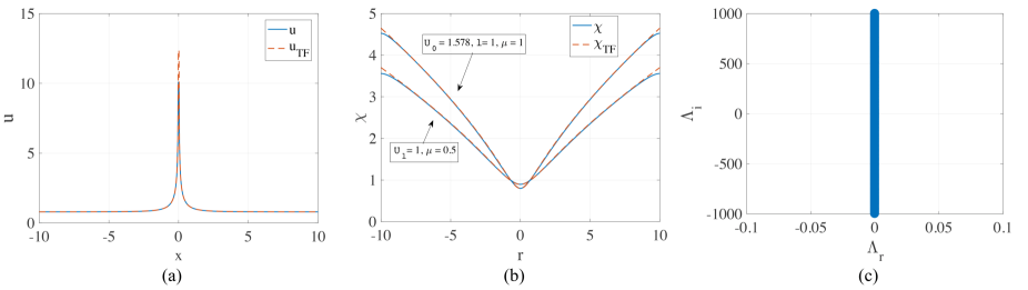
Figure 1: (a) The profile of the singular state, produced by the numerical solution of Eq. (12) with $\alpha=3$ and $k=0$, and its counterpart, predicted by the TF approximation (33), for $U_{l}=1$ and $\mu=0.5$. (b) The lower curves are the same as (a), shown in terms of function $\chi(r)$, see Eq. (19). The upper curves in (b) show an example of a stable singular vortex, taken at values of parameters close to the stability boundary given by Eq. (29): $l=1$, $\mu=1$, and $U_{0}=1.578$, while the boundary value is $\left(U_{0}\right)_{\min}=1.556$. (c) The spectrum of the stability eigenvalues for the singular vortex corresponding to the upper plots in (a), as produced by the numerical solution of BdG equations (LABEL:BdG).

Further, up to the numerical accuracy, the results obtained for the stability of the singular states exactly agree with the analytical stability condition given by Eq. (29). This conclusion is illustrated by Figs. 1(b,c) and 2, where the singular vortices with $l=1$, $\mu=1$ and spectra of their stability eigenvalues are displayed, respectively, for $U_{0}=1.578$ and $U_{0}=1.533$, while the respective stability-boundary value is $\left(U_{0}\right)_{\min}=14/9\approx\allowbreak 1.556$. It is seen that, accordingly, the former solution is stable, while the latter one is not. Additionally, Fig. 2(c) displays the trajectory of spontaneous motion of the pivot caused by the drift instability of the stationary vortex shown in Fig. 2(a). The drift character of the instability complies with the fact that the unstable eigenvalues, shown in panel 2(b), are produced by small perturbations with $m=1$ in Eq. (22).

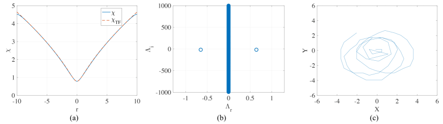
Figure 2: (a,b) The same as in Figs. 1(b,c), but for $U_{0}=1.533$. This state is unstable, in agreement with Eq. (29). Panel (c) shows the trajectory of spontaneous motion of the vortex' pivot, produced by simulations of Eq. (10) for total evolution time $t=300$.

Numerical results confirm as well the existence of the “counter-intuitive" singular antidark modes in interval (9). An example, and its comparison to the TF approximation, as given by Eq. (33), are displayed in Fig. 3. In particular, the zoom of a segment of the modal profile shown in panel (c) clearly confirms the existence of a shallow local minimum of $u(r)$. As mentioned above, this feature is made necessary by the impossibility to directly match the asymptotic form of the singularity, given by Eq. (15), and the asymptotic expansion (14) at $r\rightarrow\infty$. The singular states with $l=0$ are stable in interval (9), while their counterparts with $l\geq 1$ are not, in accordance with Eq. (29).

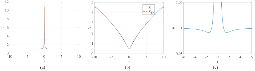
Figure 3: Panels (a) and (b): the same as in Figs. 1(a,b), but for $l=0$, $\mu=1$, and $U_{0}=-0.2$ (this value belongs to interval (9)). Panel (c) shows a shallow local minimum in the numerically found radial profile of the solution. This state is stable, as are all solutions with $l=0$ belonging to interval (9).

The above singular states are produced by setting $k=0$ in Eqs. (10) and (12), as the HO trapping potential does not play a significant role for the singular states. On the other hand, the HO potential produces an essential effect if applied to the flat-vortex mode (16), since it distorts the flat profile, as shown in Fig. 4. Note that the width of the profile is close to that of the GS wave function of the linearized equation, given by Eq. (17), while its amplitude is accurately predicted by the TF approximation, which yields $u_{\mathrm{TF}}(x=0)=\mu^{1/3}\approx 1.59$ in this case.

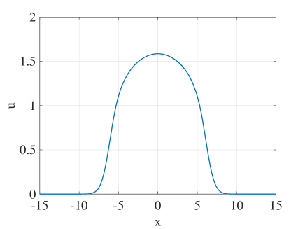
Figure 4: The numerically found profile of the intermediate vortex model with $U_{l}=0$ (the one which has the flat profile (16) in the absence of the HO potential), for $\mu=4$, $k=0.2$, and $\alpha=3$.

III.2 Excitation of singular vortices by regular vortex inputs

An issue which is crucially important for the possibility of the creation of singular (antidark) vortices in the experiment, using the nonlinear light propagation and BEC alike, is a scenario for the excitation of such “extraordinary" modes, as incident optical beams, which are employed for the creation of the usual photonic Swartz -opt-review3 , Neshev ; Segev and matter-wave vort-excit1 ; vort-excit2 , BEC-review1 -BEC-review3 vortices, may carry only the ordinary (nonsingular) vorticity.

Thus, it is relevant to simulate Eq. (10) with $U_{0}>0$ and the input taken as a usual vortex beam, i.e., a stationary solution of the linearized version of Eq. (10) with $U_{0}=0$:

$$\psi_{0}\left(r,\theta\right)=a_{0}r^{l}e^{il\theta}\exp\left(-\frac{1}{2}\sqrt{k}r^{2}\right),$$ (40)

where $a_{0}$ is an arbitrary constant. To the best of our knowledge, such simulations were not reported in previous works. Note that input (40) cannot generate an ordinary (dark nonsingular) vortex state, as it does not exist in the case of $U_{0}>0$, according to Eq. (39).

Direct simulations of Eq. (10) readily confirm that, at all values $U_{0}>0$, and for both nonlinearities considered here, which correspond to $\alpha=3$ and $4$, initial condition (40) gives rise to perturbed vortex states, close to the expected singular ones, which keep the initial vorticity, $l$. A typical example is presented in Fig. 5, which displays amplitude profiles of the input and output vortex modes (panels (a) and (c), respectively) and the overall image of the spatiotemporal evolution from the regular initial condition to a quasi-singular output, shown by means of the radial cross section in panel (b).

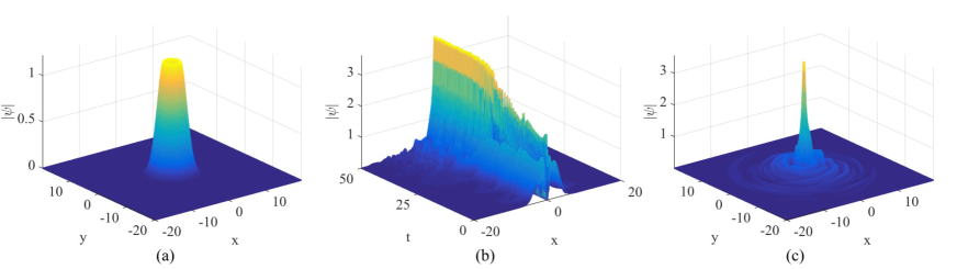
Figure 5: Creation of a singular vortex in simulations of Eq. (10), with $U_{0}=4$, $k=0.1$, and $\alpha=3$, from the regular-vortex input taken as per Eq. (40) with $l=1$ and total norm $N=40$ (see Eq. (6)), which corresponds to $a_{0}=2/\sqrt{\pi}\approx 1.13$ in Eq. (40). Panels (a) and (c): amplitude profiles of the input (at $t=0$) and output (at $t=50$), respectively. The intermediate panel (b) displays the spatiotemporal evolution of $\left|\psi\left(x,t\right)\right|$ in cross section $y=0$.

In Fig. 5(c), it is observed that the emerging central singular vortex (in the simulation, its amplitude remains finite due to the effect of the Cartesian numerical mesh) is surrounded by an additional set of radial waves. The central core and radial undulations are separated by a zero-amplitude ring, whose radius may be predicted by the TF approximation, applied to Eq. (12) with $\mu=0$. Indeed, such an approximation predicts $u(r)=0$ at $r_{0}=\left(U_{l}/k\right)^{1/4}$. For parameters of Fig. 5, this formula yields $r_{0}\approx 2.34$, which is close to the zero-amplitude radius observed in Fig. 5(c).

The fact that the simulations displayed in Fig. 5 were performed in the Cartesian coordinates explains some deviation from the axial symmetry observed in the figure (in particular, the pivot of the emerging singular vortex is somewhat shifted off the central point and performs circular motion around it). The simulations used an absorber installed at edges of the spatial domain. As a result, about $2\%$ of the initial norm was lost in the course of the simulations, by $t=50$.

III.3 Regular dark vortices

We address the regular dark modes, first, in the case of the repulsive central potential, i.e., $U_{0}<0$, with $l=0$ and $1$, supported by the flat background (14) in the absence of the HO trapping potential, $k=0$. Different values of $U_{0}$ and $l$, which amount to the same value of combination (5), give rise to identical shapes of the modes (while their stability depends on $U_{l}$ and $l$ separately, as shown below). In Fig. 6 we plot a set of profiles of the dark modes produced by the numerical solution of Eq. (12) for a fixed value of the chemical potential, $\mu=0.5$, and three different values of $U_{l}$, viz., $-1$, $-2$, and $-3$. In the same figure, the numerically found profiles are compared to the TF approximation, as given by Eq. (38).

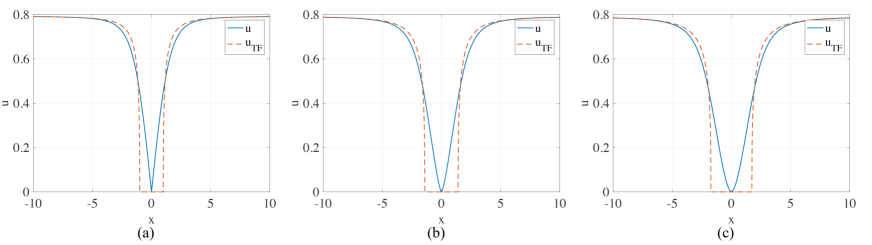
Figure 6: Shapes of dark regular modes produced by the numerical solution of Eq. (12) with $k=0$ (no HO trap), $\alpha=3$, $\mu=0.5$ and $U_{l}=-1$ (a), $-2$ (b), and $-3$ (c). Their counterparts produced by the TF approximation based on Eq. (38) are shown too.

Both the calculation of the stability eigenvalues through the numerical solution of Eq. (LABEL:BdG) and direct simulations demonstrate that all the dark modes with $l=0$ and $1$ are stable as solutions of Eq. (10) with $U_{0}<0$ and $k=0$. An example is presented in Fig. 7, which demonstrates the shape, spectrum of eigenvalues, and perturbed evolution of a typical solution of such a type.

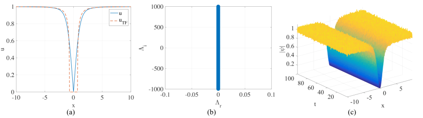
Figure 7: (a) The numerically found shape of the dark mode, obtained as a solution of Eq. (12) with $k=0$ (no HO trapping potential), $\alpha=3$, $U_{0}=-1$, $l=0$, and $\mu=1$. Its TF counterpart is displayed too, as produced by Eq. (38). (b) The spectrum of stability eigenvalues for small perturbations around this mode, $\Lambda\equiv\Lambda_{\mathrm{r}}+i\Lambda_{\mathrm{i}}$, as produced by the numerical solution of the respective BdG equations. The spectrum includes no unstable eigenvalues with $\Lambda_{\mathrm{r}}\neq 0$. (c) The simulated evolution of the same mode, with $5\%$ initial random perturbations added to it, confirms its stability.

As mentioned above, the dark vortex with $l\geq 1$ may exist in the case of the attractive central potential, viz., at

$$0<U_{0}<l^{2},$$ (41)

which corresponds to $0<-U_{l}<l^{2}$, as per Eq. (5). Even for the simplest case of $l=1$, results for the stability are complicated in this case. The numerical analysis performed for $l=1$ reveals an alternation of stability and instability regions in the interval of $0<U_{0}<1$. The analysis was performed with the inclusion of a weak but finite trapping HO potential in Eqs. (10), (12), and the corresponding BdG equations, as, in the absence of the trap, the necessity to maintain the vortical boundary conditions at $r\rightarrow\infty$ makes it difficult to solve the stability problem, cf. work HanPu . As an example, Fig. 8 presents the shape and spectrum of the stability eigenvalues for the dark vortex, as obtained at a small positive value of the attraction strength, $U_{0}=0.03$, with $\mu=1$ and a weak trapping potential, corresponding to $k=0.02$ in Eq. (10).

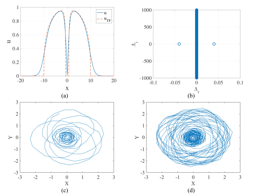
Figure 8: Panels (a) and (b) show the same as (a) and (b) in Fig. 7, but for an unstable dark vortex, produced by the numerical solution of Eqs. (12) and (LABEL:BdG) with $U_{0}=0.03$, $k=0.02$, for $l=1$ and $\mu=1$. The TF profile in (a) is produced by Eqs. (35) and (37). The unstable pair of eigenvalues in (b) corresponds to the azimuthal perturbation index $m=1$, cf. Eq. (22). Trajectories of the motion of the central point (pivot) of an unstable dark vortex from (a), as produced by simulations of Eq. (10) with total evolution time $t=1000$ and $4000$ are displayed in (c) and (d), respectively.

The instability represented by the pair of real eigenvalues in Fig. 8(b) corresponds to azimuthal index $m=1$ of small perturbations, cf. Eq. (22), which, as said above, implies the drift instability. In accordance with the expectation, in direct simulations the pivot of the unstable dark vortex spontaneously starts motion along a spiral-like unwinding trajectory, which however, remains trapped in the area of $r<r_{\mathrm{trap}}=k^{-1/4}\approx 2.7$, where $r_{\mathrm{trap}}$ is the trapping radius imposed by the HO potential, see Eq. (17). Motion of the pivot along the confined trajectory of an apparently irregular shape was going on as long as the simulations were running.

In interval (41) corresponding to $l=1$, i.e., $0<U_{0}<1$, the calculation of stability eigenvalues produced by the numerical solution of the BdG equations produces a complex structure (feasibly, a fractal one) of alternating stability and instability windows, as shown in Fig. 9. This structure is confined to two sub-intervals, viz., $0.01<U_{0}<0.17$ and $0.43<U_{0}<1$.

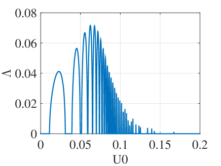
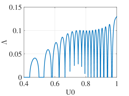
Figure 9: The real instability growth rate, $\Lambda$, for the dark-vortex mode with $l=1$, $\mu=1$ and $m=1$, cf. Eq. (22), produced by the numerical solution of the BdG equations, vs. strength $U_{0}$ of the pulling-to-the-center potential (2). The strength of the HO trapping potential is fixed as $k=0.02$. Panels (a) and (b) show two instability regions, which are, approximately, $0.01<U_{0}<0.17$ and $0.43<U_{0}<1$.

The complex structure observed in Fig. 9 may be interpreted as a result of interplay and possible resonance between two basic oscillatory modes admitted by the GP equation (10). This possibility is suggested by the affinity of the dynamical setting under the consideration to a similar 1D system, in which the counterpart of the dark vortex state with $l=1$ is the dark soliton Dimitri . In the 1D case, one basic mode represents collective dipole oscillations of the condensate as a whole (“sloshing") in the HO trap dipole-mode1 ; dipole-mode2 , while the other mode amounts to oscillatory motion of the dark soliton under the action of the same trapping potential dark-sol1 ; dark-sol2 . The possibility of producing complex dynamics by the interplay of these 1D modes was demonstrated in various setups sol-dipole1 ; sol-dipole2 ; Newcastle . In the present 2D situation, perusal of the simulations demonstrates that the quasi-spiral motion of the vortex' pivot, in the case of the instability of the stationary vortex, is indeed coupled to sloshing-rotating motion of the trapped condensate as a whole, therefore the resonance between the circular motion of the vortex displaced from the center and the collective oscillatory-rotational motion of the condensate is a feasible cause of the complex structure displayed in Fig. 9. Detailed analysis of this conjecture should be a subject of a separate work.

Another essential point of the analysis is instability of double dark vortices, with $l=2$, against splitting into unitary ones, which occurs in many models supporting dark vortex modes HanPu ; Neu ; Kawaguchi ; Finland ; Delgado ; Poland . In this case too, the HO trapping potential should be kept in Eq. (10), to secure the robustness of the numerical scheme (cf. a similar situation in the case of the 2D GP equation with the cubic term HanPu ). A weak trap with $k=0.02$ is sufficient to support stable double vortices at particular values of $U_{0}$ and $\mu$, provided that $U_{l}$ is negative, see Eq. (5). An example of the profile of a stable dark double vortex and its stable perturbed propagation is presented in Fig. 10.

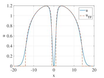
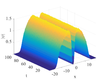
Figure 10: (a) The numerically found profile of a stable dark vortex with $l=2$ and $\mu=2$, obtained at $U_{0}=0$ (hence, $U_{l}=-4$), $k=0.02$, and $\alpha=3$ in Eq. (10). The TF counterpart of this profile, produced by Eqs. (35) and (37), is shown too. (b) Stable evolution of this double vortex with initially added random perturbations.

The increase of the chemical potential from $\mu=2$, corresponding to the stable double vortex in Fig. 10, to $\mu=3.2$ makes the dark double vortex unstable against perturbations with azimuthal index $m=2$, cf. Eq. (22). The vortex' profile and spectrum of the respective (in)stability eigenvalues are displayed in Fig. 11.

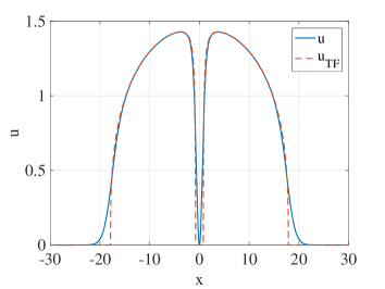
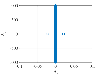
Figure 11: The same as in Figs. 8(a,b), but for the unstable double dark vortex ($l=2$), with $\mu=3.2$. The parameters are the same as in Fig. 10: $U_{0}=0$, $k=0.02$, $\alpha=3$. The unstable pair of eigenvalues corresponds to the azimuthal perturbation index $m=2$, cf. Eq. (22). There are no unstable eigenvalues with $m=1$.

Because the instability of the double vortex in Fig. 11 is driven by the perturbation eigenmode with azimuthal index $m=2$, it splits the initial vortex ring into a pair of unitary vortices. As shown in Fig. 12, the splitting is followed by recombination back into the original vortex, thus initiating a periodic chain of splittings and recombinations. Simultaneously, the vortex pair in the split state rotates persistently.

Unlike the motion of the unstable vortex with $l=1$, which is shown above in Figs. 8(c,d), the periodic fission-fusion evolution of the double vortex, presented in Fig. 12, is not coupled to conspicuous sloshing motion of the condensate as a whole. This circumstance may be explained by the fact that monopole modes of stirring perturbations, produced by the motion of two unitary vortices (separated by a relatively small distance in Fig. 12) in opposite directions, cancel each other through destructive interference. The remaining dipole stirring mode produces a much weaker sloshing effect.

At other parameter values, another instability eigenmode of a double vortex is possible. An example of such a vortex is shown in Fig. 13. In this case, the instability corresponds to azimuthal index $m=1$ (rather than $m=2$). Accordingly, direct simulations displayed in Fig. 14 show that the double vortex splits in a pair of unitary vortices. One of them is expelled from the central position first, which is later followed by the expulsion of the second one.. Both secondary vortices perform persistent orbital motion in a confined region. Unlike what is observed in Fig. 12, the splitting is irreversible in Fig. 14 i.e., the unitary vortices never recombine back into a single double vortex.

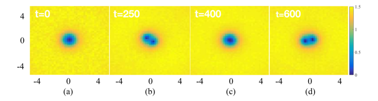
Figure 12: A set of snapshots illustrating the evolution of the unstable dark double vortex from Fig. 11. It features a periodic chain of splittings into a rotating pair of unitary vortices (as observed at $t=250$ and $600$), alternating with recombinations back into the double vortex (as seen at $t=0$ and $400$).

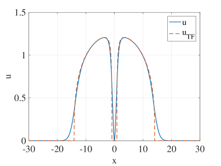
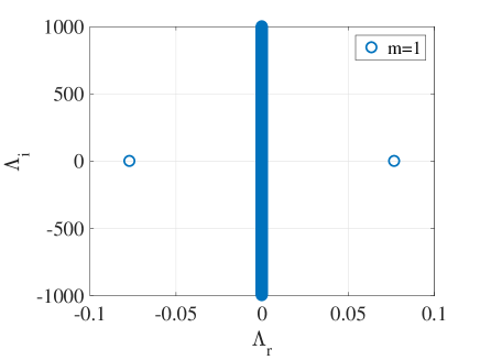
Figure 13: The same as in Fig. 11, but for the unstable double dark vortex ($l=2$), with $\mu=2$, $U_{0}=1$, $k=0.02$, and $\alpha=3$. (b) The spectrum of stability eigenvalues, the unstable real pair corresponding to the azimuthal perturbation index $m=1$, cf. Eq. (22). There are no unstable eigenvalues for $m=2$.

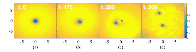
Figure 14: A set of snapshots illustrating the evolution of the unstable dark double vortex from Fig. 13. It splits in two separate unitary vortices, which are expelled from the center one by one, performing circular motion in a confined region.

The alternation of stability and instability regions for the double vortices, following the variation of $U_{0}$, forms a complex structure, which is plotted in Fig. 15, separately for eigenmodes with the azimuthal index $m=2$ in (a), and $m=1$ in (b). Note that there is no instability at $U_{0}<-1/2$, and the dark double vortex does not exist at $U_{0}\geq 4$. The structure observed in the figure may be interpreted as a result of the interplay and possible resonance between two oscillatory modes. One represents internal oscillations in the pair of separated unitary vortices, while the other mode corresponds to rotation of the vortex pair.

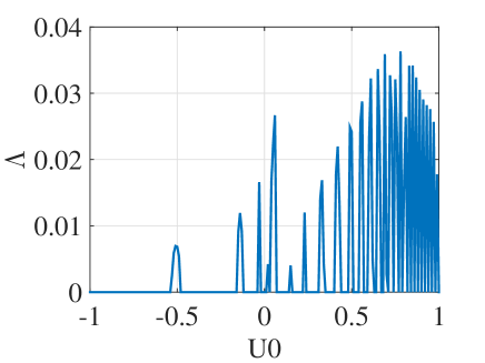
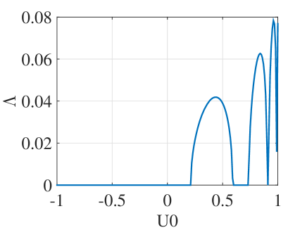
Figure 15: The instability growth rate for the dark double vortex vs. strength $U_{0}$ of the central potential (2), at fixed values of the trapping potential in Eq. (10), $k=0.02$ (with $\alpha=3$), and chemical potential, $\mu=2$, for azimuthal perturbation indices $m=2$ (a), and $m=1$ (b), cf. Eq. (22).

IV Conclusion

The main objective of this work is to extend the family of singular but physically relevant singular vortices in the 2D models of optical and matter waves, which combine attractive potential (2) and the quartic ($\alpha=3$) or quintic ($\alpha=4$) self-repulsion in Eq. (10), for the antidark vortex states built on top of a finite background. It is demonstrated that the TF (Thomas-Fermi) approximation provides a very accurate fit for the numerically found singular states. Their stability exactly follows the recently proposed analytical condition, given by Eq. (29) for $\alpha=3$, and by the newly derived Eq. (31) for $\alpha=4$. A nontrivial finding is the existence of the singular states in the case when the effective potential strength, given by Eq. (5), is negative, corresponding to weak repulsion, instead of the pull to the center. In this case, the shape of the mode features a shallow local minimum, as shown in Fig. 3(c). An essential novel result is the scenario for the excitation of perturbed singular vortices by the ordinary (nonsingular) vortex input, which is shown in Fig. 5. Parallel to that, the analysis is performed for the usual regular (dark) vortices, which are also supported by a finite background, in the case when the effective central potential is repulsive. The dark states with vorticities $l=0$ and $1~{}$are completely stable for $U_{0}<0$ in Eq. (2)). In the interval of $0<U_{0}<1$, where the effective potential's strength, including the centrifugal term, $U_{0}-1$, corresponds to the repulsion, the accurate stability analysis for the dark vortex with $l=1$ is possible in the presence of the weak confining HO (harmonic-oscillator) potential. In this case, the vortex features an intricate pattern of alternating stability and instability windows, as shown in Fig. 9. Unstable vortices spontaneously move along complex trajectories, which do not leave the central area confined by the HO trap (an example is displayed in Fig. 8 (c) and (d)). The presence of the weak trap is also necessary for the accurate analysis of the stability of dark double vortices. In this case too, stability and instability regions compose a complex pattern. Unstable double vortices periodically split into rotating pairs of unitary vortices and recombine back. Finally, simple but new solutions for flat vortices are obtained at the border between the antidark singular vortices and dark regular ones.

A challenging direction for extension of the present work may be the analysis of antidark vortex states in the 3D model with the same central potential.

References

- (1) Swartzlander G A and Law C T, Optical vortex solitons observed in Kerr nonlinear media 1992 Phys. Rev. Lett. 69, 2503-2506.
- (2) Soskin M S and Vasnetsov M V, Singular optics, 2001 Prog. Opt. 42, 219-275.
- (3) Desyatnikov A S, Torner L, and Kivshar Y S, Optical vortices and vortex solitons, 2005 Prog. Opt. 47, 291-391.
- (4) Franke-Arnold S, Allen L, and Padgett M, Advances in optical angular momentum, 2008 Laser & Photon. Rev. 2, 299–313 (2008).
- (5) Malomed B A, Vortex solitons: Old results and new perspectives, 2019, Physica D 399, 108-137.
- (6) Shen Y, Wang X, Xie Z, Min C, Fu X, Liu Q, Gong M, and Yuan X, Optical vortices 30 years on: OAM manipulation from topological charge to multiple singularities 2019 Light: Science & Applications 8, 90
- (7) Kasamatsu K, Tsubota M, and Ueda M, Vortices in multicomponent Bose-Einstein condensates, 2005 Int. J. Mod. Phys. B 19, 1835-1904.
- (8) Srinivasan R, Vortices in Bose-Einstein condensates: A review of the experimental results, 2006 Pramana J. Physics 66, 3-30.
- (9) Fetter A L, Rotating trapped Bose-Einstein condensates, 2009 Rev. Mod. Phys. 81, 647-691.
- (10) Pitaevskii L and Stringari S. Bose–Einstein Condensation (Clarendon: Oxford, UK, 2003).
- (11) Sakaguchi H and Malomed B A, Suppression of the quantum-mechanical collapse by repulsive interactions in a quantum gas, 2011 Phys. Rev. A 83, 013607.
- (12) Shamriz E, Chen Z, and Malomed B A, Suppression of the quasi-two-dimensional quantum collapse in the attraction field by the Lee-Huang-Yang effect, 2020 Phys. Rev. A 101, 063628.
- (13) Shamriz E, Chen Z, Malomed B A, and Sakaguchi H, Singular mean-field states: a brief review of recent results, 2020 Condensed Matter 5, 20.
- (14) Yan L, Xu G-Y, Wang Y-J, Liu X-F, and Han J-R, Dynamics of an ultracold Bose Gas in funnel-shaped potential, 2009, Commun. Theor. Phys. 52, 431-434.
- (15) dos Santos M, Malomed B, and Cardoso W, Quasi-one-dimensional approximation for Bose-Einstein condensates transversely trapped by a funnel potential, 2019, J. Phys. B: At., Mol & Opt. Phys. 52, 245301.
- (16) dos Santos M C P, Malomed B A, and Cardoso W B, Double-layer Bose-Einstein condensates: A quantum phase transition in the transverse direction, and reduction to two dimensions, 2020, Phys. Rev. E 102, 042209.
- (17) Landau L D and Lifshitz E M, Quantum Mechanics (Elsevier: Amsterdam, 1977).
- (18) Michinel H, Campo-Taboas J, Garcia-Fernandez R, Salgueiro J R, and Quiroga-Teixeiro M L, Liquid light condensates, 2002, Phys. Rev. E 65, 066604.
- (19) Boudebs G, Cherukulappurath S, Leblond H, Troles J, Smektala F, and Sanchez F, Experimental and theoretical study of higher-order nonlinearities in chalcogenide glasses, 2003, Opt. Commun. 219, 427-433.
- (20) Bigelow M S, Zerom P, and Boyd R W, Breakup of ring beams carrying orbital angular momentum in sodium vapor, 2004, Phys. Rev. Lett. 92, 083902.
- (21) Konar S, Mishra M and Jana S, Nonlinear evolution of cosh-Gaussian laser beams and generation of flat top spatial solitons in cubic quintic nonlinear media, 2007, Phys. Lett. A 362, 505-510.
- (22) Reyna A S and de Araújo C B, High-order optical nonlinearities in plasmonic nanocomposites – a review, 2017 Adv. Opt. Phot. 9, 720-774.
- (23) Gammal A, Frederico T, Tomio L, and Abdullaev F K, Stability analysis of the D-dimensional nonlinear Schrödinger equation with trap and two- and three-body interactions, 2000, Phys. Lett. A 267, 305-311.
- (24) Petrov D S, Quantum mechanical stabilization of a collapsing Bose-Bose mixture, 2015 Phys. Rev. Lett. 115, 155302.
- (25) Petrov D S and Astrakharchik G E, Ultradilute low-dimensional liquids, 2016 Phys. Rev. Lett. 117, 100401.
- (26) Żin P, Pylak M, Wasak T, Gajda M, and Idziaszek Z, Quantum Bose-Bose droplets at a dimensional crossover, 2018, Phys. Rev. A 98, 051603(R).
- (27) Ilg T, Kumlin J, Santos L, Petrov D S, and Büchler H P, Dimensional crossover for the beyond-mean-field correction in Bose gases, 2018, Phys. Rev. A 98, 051604.
- (28) Cabrera C, Tanzi L, Sanz J, Naylor B, Thomas P, Cheiney P, and Tarruell L, 2018, Quantum liquid droplets in a mixture of Bose-Einstein condensates, Science 359, 301-304.
- (29) Cheiney P, Cabrera C R, Sanz J, Naylor B, Tanzi L, and Tarruell L, Bright soliton to quantum droplet transition in a mixture of Bose-Einstein condensates, 2018, Phys. Rev. Lett. 120, 135301.
- (30) Semeghini G, Ferioli G, Masi L, Mazzinghi C, Wolswijk L, Minardi F, Modugno M, Modugno G, Inguscio M, and Fattori M, 2018, Self-bound quantum droplets of atomic mixtures in free space, 2018 Phys. Rev. Lett. 120, 235301.
- (31) Ferioli G, Semeghini G, Masi L, Giusti G, Modugno G, Inguscio M, Gallemi A, Recati A, and Fattori M, Collisions of self-bound quantum droplets, 2019 Phys. Rev. Lett. 122, 090401.
- (32) D'Errico C, Burchianti A, Prevedelli M, Salasnich L, Ancilotto F, Modugno M, Minardi F, and Fort C, Observation of quantum droplets in a heteronuclear bosonic mixture, 2019 Phys. Rev. Res. 1, 033155.
- (33) Manini N and Salasnich L, Bulk and collective properties of a dilute Fermi gas in the BCS-BEC crossover, 2005, Phys. Rev. A 71, 033625.
- (34) Bulgac A, Local-density-functional theory for superfluid fermionic systems: The unitary gas, 2007, Phys. Rev. A 76, 040502(R).
- (35) Adhikari S K, Superfluid Fermi-Fermi mixture: Phase diagram, stability, and soliton formation, 2007, Phys. Rev. A 76, 053609.
- (36) Adhikari S K, Nonlinear Schrödinger equation for a superfluid Fermi gas in the BCS-BEC crossover, 2008, Phys. Rev. A 77, 045602.
- (37) Veron L, Singular solutions of some nonlinear elliptic equations 1981 Nonlinear Anal. Theory Methods Appl. 5, 225-242.
- (38) Sakaguchi H and Malomed B A, Singular solitons, 2020 Phys. Rev. E 101, 012211.
- (39) Axisymmetric versus nonaxisymmetric vortices in spinor Bose-Einstein condensates
- (40) Lovegrove J, Borgh M O, and Ruostekoski J, Energetically stable singular vortex cores in an atomic spin-1 Bose-Einstein condensate, 2012, Phys. Rev. A 86, 013613.
- (41) Ponomarenko S A, Huang W, and Cada M, Bark and antidark diffraction-free beams, 2007, Opt. Lett. 32, 2508-2510.
- (42) Xu T, Li M, and Li L, Anti-dark and Mexican-hat solitons in the Sasa-Satsuma equation on the continuous wave background, 2015, EPL 109, 30006.
- (43) Horikis T P and Frantzeskakis D J, Ring dark and antidark solitons in nonlocal media, 2016, Opt. Lett. 41, 583-586.
- (44) Jørgensen N B, Bruun G M, and Arlt J J, Dilute fluid governed by quantum fluctuations, 2018 Phys. Rev. Lett. 121, 173403.
- (45) Raghavan S and Agrawal G P, Spatiotemporal solitons in inhomogeneous nonlinear media, 2000, Opt. Commun. 180, 377-382.
- (46) Pu H, Law C K, Eberly J H, and Bigelow N P, Coherent disintegration and stability of vortices in trapped Bose condensates, 1999 Physical Review A 59, 1533-1537.
- (47) Patil S H, Susceptibility and polarizability of atoms and ions, 1985, J. Chem. Phys. 83, 5764-5771.
- (48) Putz M V, Russo N, and Sicilia E, Atomic radii scale and related size properties from density functional electronegativity formulation 2003, J. Phys. Chem. A 107, 5461-5465.
- (49) Rokhsar D S, Vortex stability and persistent currents in trapped Bose gases, 1997, Phys. Rev. Lett. 79, 2164-2167.
- (50) Neu J C, Vortices in complex scalar fields, 1990 Physica D 43, 385-406.
- (51) Kawaguchi Y and Ohmi T, Splitting instability of a multiply charged vortex in a Bose-Einstein condensate, 2004, Phys. Rev. A 70, 043610.
- (52) Huhtamäki J A M, Möttönen M, Isoshima T, Pietilä V, and Virtanen S M M, Splitting times of doubly quantized vortices in dilute Bose-Einstein condensates, 2006, Phys. Rev. Lett. 97, 110406.
- (53) Muñoz Mateo A and Delgado V, Dynamical evolution of a doubly quantized vortex imprinted in a Bose-Einstein condensate, 2006, Phys. Rev. Lett. 97, 180409.
- (54) Gawryluk K, Karpiuk T, Brewczyk M, and Rzażewski K, Splitting of doubly quantized vortices in dilute Bose-Einstein condensates, 2008 Phys. Rev. A 78, 025603.
- (55) Neshev D N, Alexander T J, Ostrovskaya E A, Kivshar Y S, Martin H, Makasyuk I, and Chen Z G, Observation of discrete vortex solitons in optically induced photonic lattices, 2004, Phys. Rev. Lett. 92, 123903.
- (56) Fleischer J W, Bartal G, Cohen O, Manela O, Segev M, Hudock J, and Christodoulides D N, Observation of vortex-ring “discrete” solitons in 2D photonic lattices, 2004, Phys. Rev. Lett. 92 (2004) 123904.
- (57) Madison K W, Chevy F, Bretin V, and Dalibard J, Stationary states of a rotating Bose-Einstein condensate: Routes to vortex nucleation, 2001, Phys. Rev. Lett. 86, 4443-4446.
- (58) Raman C, Abo-Shaeer J R, Vogels J M, Xu K, and Ketterle W, Vortex nucleation in a stirred Bose-Einstein condensate, 2001, Phys. Rev. Lett. 87, 210402.
- (59) Frantzeskakis D J, Dark solitons in atomic Bose–Einstein condensates: from theory to experiments, 2010, J. Phys. A: Math. Theor. 43, 213001.
- (60) Morgan S A, Ballagh R J, and Burnett K, Solitary-wave solutions to nonlinear Schrödinger equations, 1997, Phys. Rev. A 55, 4338.
- (61) Muryshev A E, van Linden van den Heuvell H B, and Shlyapnikov G V, Stability of standing matter waves in a trap, 1999, Phys. Rev. A 60, R2665.
- (62) Busch Th and Anglin J R, Motion of dark solitons in trapped Bose-Einstein condensates, 2000, Phys. Rev. Lett. 84, 2298.
- (63) Huang G, Szeftel J, and Zhu S, Dynamics of dark solitons in quasi-one-dimensional Bose-Einstein condensates, 2002, Phys. Rev. A 65, 053605.
- (64) Parker N G, Proukakis N P, Leadbeater M, and Adams C S, Soliton-sound interactions in quasi-one-dimensional Bose-Einstein condensates, 2003, Phys. Rev. Lett. 90, 220401.
- (65) Parker N G, Proukakis N P, and Adams C S, Dark soliton decay due to trap anharmonicity in atomic Bose-Einstein condensates, 2010, Phys. Rev. A 81, 033606.
- (66) Bland T, Parker N G, Proukakis N P, and Malomed B A, Probing quasi-integrability of the Gross-Pitaevskii equation in a harmonic-oscillator potential, 2018, J. Phys. B: At. Mol. Opt. Phys. 51, 205303.