Cyclotrons and Fixed Field Alternating Gradient Accelerators

Abstract

Due to its simplicity the classical cyclotron has been used very early for applications in science, medicine and industry. Higher energies and intensities were achieved through the concepts of the sector focused isochronous cyclotron and the synchro-cyclotron. Besides those the fixed field alternating gradient accelerator (FFA) represents the most general concept among these types of fixed field accelerators, and the latter one is actively studied and developed for future applications.

1 Introduction

Cyclotrons have a long history in accelerator physics and are used for a wide range of medical, industrial, and research applications [onishenko, seidel_cal]. The first cyclotrons were designed and built by Lawrence and Livingston [lawrence, livingston] back in 1931. The cyclotron represents a resonant-accelerator concept. Due to the repeated acceleration process it is possible to achieve relatively high kinetic energies while the required voltages stay in a moderate range. Historically that was a major advantage over single pass high voltage accelerators. Furthermore, several properties such as CW operation make the concept well suited for the acceleration of hadron beams with high average intensity. Relativistic effects limit the energies in reach for the classical cyclotron concept. These limitations were overcome to some degree by the sector focused isochronous cyclotron, that allows to accelerate protons to a range of $\approx 1\,$GeV. Another approach for reaching such energies is the synchro-cyclotron, that involves cycling of the RF frequency at the expense of a lower average beam intensity. Scaling and non-scaling FFA utilize strong focusing to reduce the radial orbit variation. In a sense FFA concepts represent a generalisation of the cyclotron. As a major difference to synchrotrons the magnetic fields of FFA’s and cyclotrons are not cycled during acceleration, and thus higher average intensities can be achieved.

2 Cyclotron Concepts

Although the classical cyclotron has major limitations and is practically outdated today, some fundamental relations are best explained within this original concept. In the classical cyclotron an alternating high voltage at radio frequency (RF) is applied to two D-shaped hollow electrodes, the Dees, for the purpose of acceleration. Ions from a central ion source are repeatedly accelerated from one dee to the other. The ions are kept on a piecewise circular path by the application of a uniform, vertically oriented magnetic field. On the last turn, the ions are extracted by applying an electrostatic field using an electrode. The concept is illustrated in Fig. 1.

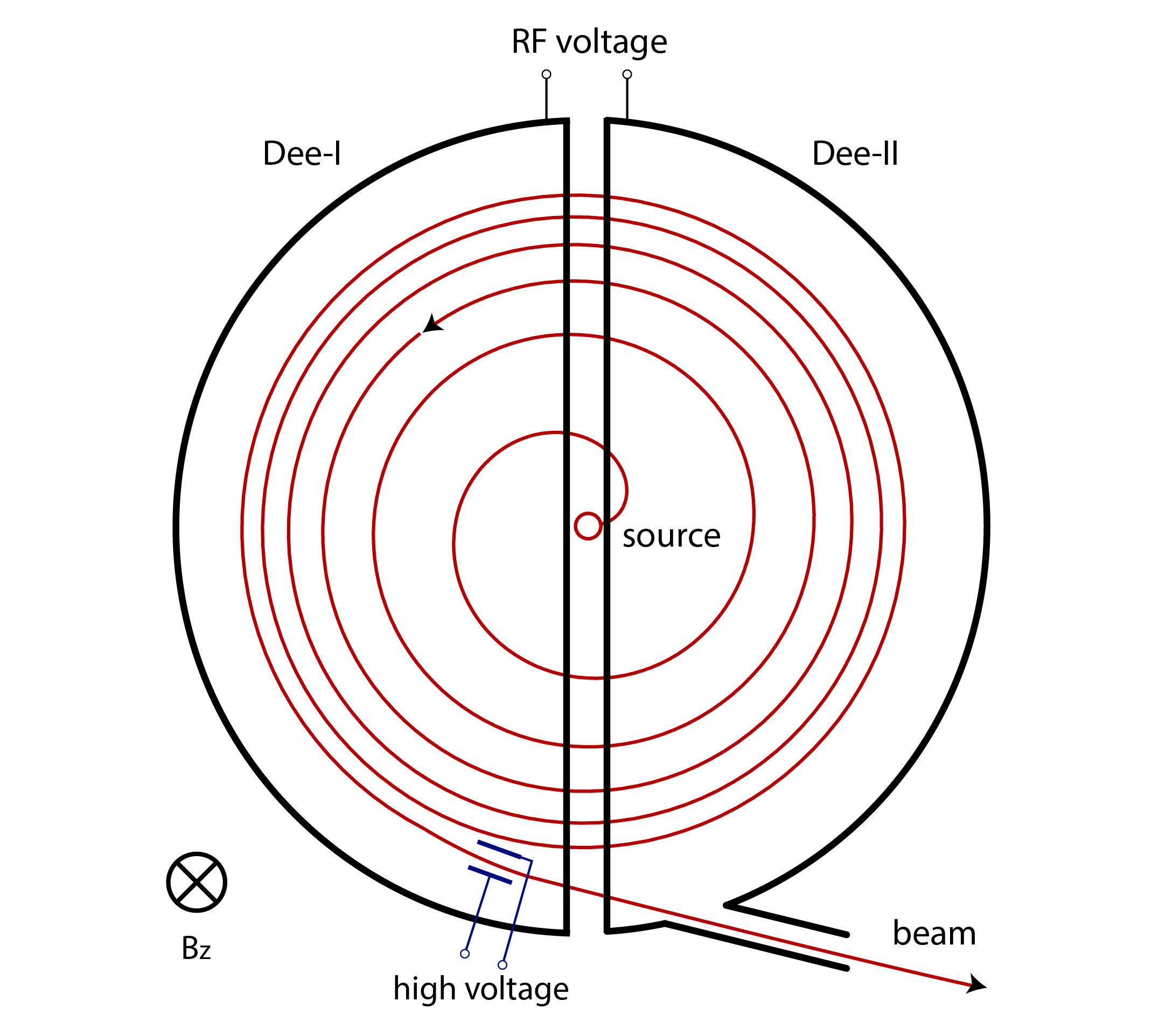
Figure 1: Conceptual sketch of a classical cyclotron in plan view. In the non-relativistic approximation, the turn separation scales as $1/R$.

The equation of motion for a particle moving in a vertically oriented magnetic field with a momentum vector in the horizontal plane is given by:

$$m\ddot{\vec{r}}=m\,\omega^{2}\vec{r}=q\,\dot{\vec{r}}\times\vec{B}_{z}.$$ (1)

The magnetic force and centrifugal force are set equal. The solution for the particles trajectory is a circle with a bending radius $\rho$ that is constant over time: →r(t) = ρ( cosωtsinωt0 ).

For kinetic energies low compared to the rest energy the particles circulate at the cyclotron frequency, which depends on the magnetic field $B_{z}$, the charge $q$ and the rest mass $m_{0}$ of the particles:

$$\omega_{c} = \frac{qB_{z}}{m_{0}}$$

$$f_{c}=\frac{\omega_{c}}{2\pi} \approx 15.2~{}\mathrm{MHz}\cdot B_{z}\mathrm{[T]}\mathrm{~{}(\,for\,\,protons\,)}.$$ (2)

As soon as relativistic effects become important, the revolution frequency decreases with the relativistic factor $\gamma$ as:

$$\omega_{\mathrm{rev}}=\omega_{c}/\gamma\,.$$ (3)

The bending radius $\rho$ is given by the well known bending strength for charged particles:

$$B\rho\,[\mathrm{T\cdot m}] = 3.336\cdot\beta\cdot E_{\mathrm{tot}}\,[\mathrm{GeV}]$$ (4)

$$\approx 4.426\cdot\sqrt{E_{k}/m_{o}c^{2}}\,.$$

The relation is expressed in practical units and the second line is an approximation for particles with kinetic energies much lower than their rest energy. $E_{\mathrm{tot}}$ is the sum of kinetic energy $E_{k}$ and rest energy $m_{0}c^{2}$. The frequency of the accelerating voltage must be equal to the revolution frequency or an integer multiple of it, i.e., $\omega_{\mathrm{rf}}=h\omega_{\mathrm{rev}}$. The harmonic number $h$ corresponds to the number of bunches that can be accelerated in one turn. With increasing velocity, particles travel at larger radii, so that $R\propto\beta$, and the revolution time remains constant and in phase with the RF voltage. We denote the average orbit radius with $R$, which may differ from the local bending radius $\rho$ for certain field configurations. In the literature on cyclotrons the variable $R_{\infty}$ has been introduced to parametrize the dependence of the orbit radius on the particles velocity:

$$R=R_{\infty}\beta,~{}R_{\infty}=\frac{c}{\omega_{c}}\,.$$ (5)

$R_{\infty}$ is a theoretical value, the trajectory radius for a particle at infinite energy and speed of light. For low energies the condition of isochronicity is fulfilled in a homogeneous magnetic field. For relativistic particles the magnitude of the B-field has to be raised in proportion to $\gamma$ at increasing radius in order to keep the revolution time constant throughout the acceleration process. Such field shape is introduced for isochronous cyclotrons as described later in Section LABEL:sec:avf. To summarize this important result - for constant revolution frequency in a cyclotron the following scaling of orbit radius and bending field is required:

$$R\propto\beta,~{}~{}B_{z}\propto\gamma\,.$$ (6)

As we will see this field scaling contradicts the requirements of transverse focusing. The radial variation of the bending field in a cyclotron generates focusing forces. At a radius $R$, the slope of the bending field is described by the field index $k$, where

$$k=\frac{R}{B_{z}}\frac{dB_{z}}{dR}.$$ (7)

Using the proportionalities Eq. (6), the scaling of the field index under isochronous conditions can be evaluated as follows:

$$\frac{R}{B}\frac{\mathrm{d}B}{\mathrm{d}R} = \frac{\beta}{\gamma}\frac{\mathrm{d}\gamma}{\mathrm{d}\beta}$$ (8)

$$= \gamma^{2}-1.$$

Note that Eq. (8) is positive, thus isochronicity requires an increasing magnetic field towards larger radii. The radial equation of motion of a single particle can be written as

$$m\ddot{r}=mr\dot{\varphi}^{2}-qr\dot{\varphi}B_{z}.$$ (9)

We now consider small deviations around the central orbit $R$, namely $r=R+x,x\ll R$:

$$\ddot{x}+\frac{q}{m}vB_{z}(R+x)-\frac{v^{2}}{R+x} = 0,$$

$$\ddot{x}+\frac{q}{m}v\left(B_{z}(R)+\frac{\mathrm{d}B_{z}}{\mathrm{d}R}x\right)-\frac{v^{2}}{R}\left(1-\frac{x}{R}\right) = 0,$$

$$\ddot{x}+\omega_{\mathrm{rev}}^{2}(1+k)x = 0.$$ (10)

In this derivation, we have used the relations $\omega_{\mathrm{rev}}=qB_{z}/m\approx v/R$ and $r\dot{\varphi}\approx v$. Thus, in the linear approximation, the horizontal ‘betatron motion’ is a harmonic oscillation around the central beam orbit, $x(t)=x_{\mathrm{max}}\cos(\nu_{r}\omega_{\mathrm{rev}}t)$. The parameter $\nu_{r}$ is called the betatron tune. From Eq. (10) we see that the radial betatron tune in a classical cyclotron is given by