Random Matrix Model for Eigenvalue Statistics in Random Spin Systems

Abstract

We propose a working strategy to describe the eigenvalue statistics of random spin systems along the whole phase diagram with thermal to many-body localization (MBL) transition. Our strategy relies on two random matrix (RM) models with well-defined matrix construction, namely the mixed (Brownian) ensemble and Gaussian $\beta$ ensemble. We show both RM models are capable of capturing the lowest-order level correlations during the transition, while the deviations become non-negligible when fitting higher-order ones. Specifically, the mixed ensemble will underestimate the longer-range level correlations, while the opposite is true for $\beta$ ensemble. Strikingly, a simple average of these two models gives nearly perfect description of the eigenvalue statistics at all disorder strengths, even around the critical region, which indicates the interaction range and strength between eigenvalue levels are the two dominant features that are responsible for the phase transition.

I Introduction

Many-body localized (MBL) phaseGornyi2005 ; Basko2006 , as the only example of phase that violates eigenstate thermalization hypothesis (ETH)Deutsch ; Srednicki in an isolated quantum system, is a focus of current condensed matter physics. Modern understanding about MBL phase and its counterpart – thermal phase that respects ETH – relies on quantum entanglement. Specifically, thermal phase is ergodic with delocalized eigenstate wavefunctions, which results in extensive (volume law) entanglement between subsystems. On the contrary, MBL phase is signatured by small (area-law) entanglement. The qualitative difference in the scaling of quantum entanglement is widely used in the study of thermal-MBL transition Kjall2014 ; Geraedts2017 ; Yang2015 ; Serbyn16 ; Gray2017 ; Maksym2015 ; Kim ; Bardarson ; Abanin .

More traditionally, the thermal and MBL phase are distinguished by their eigenvalue statisticsOganesyan ; Avishai2002 ; Regnault16 ; Regnault162 ; Huse1 ; Huse2 ; Huse3 ; Garcia ; Luitz , whose mathematical foundation is laid by the random matrix (RM) theoryMehta ; Haake2001 . The eigenvalues of thermal phase are well-correlated, whose statistics divides into three Wigner-Dyson (WD) classes depending on the system’s symmetry: the Gaussian orthogonal ensemble (GOE) for orthogonal systems with time reversal symmetry, the Gaussian unitary ensemble (GUE) for those break time reversal symmetry, and Gaussian symplectic ensemble (GSE) for time-reversal invariant systems with broken spin rotational invariance. On the contrary, the eigenvalues in MBL phase are independent of each other and follows Poisson statistics. Quantitatively, the eigenvalue statistics is evaluated by the distribution of ratios between two adjacent level spacings (gaps)

$$r_{i}^{\left(n\right)}=\frac{E_{i+2n}-E_{i+n}}{E_{i+n}-E_{i}}\text{.}$$ (1)

The lowest-order one $n=1$ was proposed in Ref.[Oganesyan, ] as the standard probe for nearest level correlation, and higher order ones with $n>1$ describe level correlations on longer ranges. Compared to the more traditional quantity like level spacing $\left\{s_{i}^{\left(n\right)}=E_{i+n}-E_{i}\right\}$ or number variance $\Sigma^{2}$, spacing ratios are independent of density of states and requires no unfolding procedure, which is non-unique and may raise subtle misleading signatures in certain modelsGomez2002 .

Besides the level statistics deep in the thermal/MBL phase, there are also significant amount of works on the spectral statistics right at the critical point, or even along the whole phase diagramShukla ; Serbyn ; SRPM ; Mix ; Sierant19 ; Rao21 ; Sierant20 ; Buijsman . For example, the single-parameter Gaussian $\beta$ ensemble, which generalizes the standard Gaussian ensembles into the one with continuous Dyson index. However, as we shall see, it can not accurately account for the high-order level statistics, especially for the MBL phase. As a generalization, the two-parameter $\beta-h$ model, recently proposed in Ref.[Sierant20, ], was shown to reproduce $P\left(r^{\left(n\right)}\right)$ with high accuracy during the MBL transition, which indicates the interaction strength and range are the two dominant varying features along with the phase transition. However, the $\beta-h$ model is based on the joint probability distribution of eigenvalues, and the two parameters $\beta$ and $h$ has to be determined jointly, which is numerically difficult to achieve. This motivates us to search for a RM model that based directly on the matrix construction to reproduce the level statistics – both on short and long ranges – of random spin systems.

In this work, we propose another working strategy to reproduce $P\left(r^{\left(n\right)}\right)$ along the thermal-MBL transition in 1D random spin systems. Our strategy is based on two RM models that have well-defined parent matrix construction, i.e. the mixed ensemble (also called Brownian ensembleShukla2000 ; Shukla2005 or Rosenzweig-Porter ensembleMehta ; Shapiro ; Kravtsov2015 in the literature) and Gaussian $\beta$ ensemble, both of which incorporate the WD and Poisson distribution in a direct manner. We will show both RM models can accurately reproduce $P\left(r^{\left(1\right)}\right)$ with properly chosen model parameters, but they both show non-negligible deviations when fitting higher-order spacing ratios. Specifically, the mixed ensemble will underestimate the longer-range level correlations, while the opposite is true for $\beta$ ensemble. Surprisingly, an average distribution of these two models gives nearly perfect description for the level statistics on moderate ranges along the whole phase diagram, even at the critical region. We argue these results also suggest the strength and range of level interaction are responsible for the MBL transition, in agreement with the conclusions of earlier worksCorps ; Sierant20 .

This paper is organised as follows. Sec.II introduces the mixed ensemble and Gaussian $\beta$ ensemble. In Sec.III we use these models to fit $P\left(r^{\left(n\right)}\right)$ in an orthogonal random spin system. Particularly, we will introduce the average distribution of the two RM models, which is shown to give fairly good descriptions of $P\left(r^{\left(n\right)}\right)$ with $n>1$, even at the transition region. In Sec.IV we verify this strategy in random spin systems with unitary symmetry and quasi-periodic potential. Conclusion and discussion come in Sec. V.

II Random Matrix Models

The basic requirement for an effective RM model for thermal-MBL transition is that it should incorporate both WD (for thermal phase) and Poisson statistics (for MBL phase). To this end, the first RM model we consider is the mixed ensemble

$$M_{\alpha\rightarrow 0}\left(x\right)=xM_{\alpha}+\left(1-x\right)M_{0}.$$ (2)

where $M_{\alpha}$ with Dyson index $\alpha=1,2,4$ represents matrix in the WD class, $M_{0}$ is a diagonal matrix with random diagonals standing for Poisson ensemble, and the normalization condition is chosen to be $Tr\left(M_{\alpha/0}^{2}\right)=1$. It’s easy to see the eigenvalue statistics of $M_{\alpha\rightarrow 0}\left(x\right)$ evolves from Poisson to WD when $x$ ranges from $0$ to $1$. Unfortunately, $P\left(r^{\left(n\right)}\right)$ in the mixed ensemble lacks a compact analytical expressionSchierenberg ; Chavda ; Corps2 , so we will use numerical results instead. Specifically, we numerically generate samples of eigenvalue spectrum of Eq. (2) in the range $x\in\left(0,1\right)$ with interval $dx=0.01$, where the matrix dimension and sample number are kept to be $1000$. After sampling, we take $400$ eigenvalues in the middle of each spectrum to determine $P\left(r^{\left(n\right)}\right)$, which will be used for future fittings.

The second considered RM model is the Gaussian $\beta$ ensemble, which is an generalization of the standard WD ensembles into the one with a continuous Dyson index $\beta\in\left(0,\infty\right)$, whose joint probability distribution of the eigenvalues is,

$$P\left(\left\{E_{i}\right\}\right)\propto\prod_{i<j}\left|E_{i}-E_{j}\right|^{\beta}e^{-\beta\sum_{i}E_{i}^{2}/2}\text{.}$$ (3)

The generalized Dyson index $\beta$ essentially controls the strength of level repulsion, and the limit $\beta\rightarrow 0$ stands for the Poisson ensemble with uncorrelated eigenvalues. The $\beta$ ensemble can be generated by a tridiagonal RMBeta

$$M_{\beta}=\frac{1}{\sqrt{2}}\left(\begin{array}[]{ccccc}x_{1}&y_{1}&&&\\ y_{1}&x_{2}&y_{2}&&\\ &\begin{array}[]{ccc}\text{.}&&\\ &\text{.}&\\ &&\text{.}\end{array}&\begin{array}[]{ccc}\text{.}&&\\ &\text{.}&\\ &&\text{.}\end{array}&\begin{array}[]{ccc}\text{.}&&\\ &\text{.}&\\ &&\text{.}\end{array}&\\ &&y_{N-2}&x_{N-1}&y_{N-1}\\ &&&y_{N-1}&x_{N}\end{array}\right)$$ (4)

where the diagonals $x_{i}\,$ follow the normal distribution $\mathit{N}\left(0,2\right)$ and $y_{k}$ ($k=1,2,...,N-1$) follows the $\chi$ distribution with parameter $\left(N-k\right)\beta$. For the $\beta$ ensemble, analytical and strong numerical evidences support $P\left(r^{\left(n\right)}\right)$ to have the following compact formAtas ; Tekur ; Rao20 ; Rao202

$$P\left(\beta,r^{\left(n\right)}=r\right) = Z_{\beta}\frac{\left(r+r^{2}\right)^{\gamma}}{\left(1+r+r^{2}\right)^{1+3\gamma/2}}\text{,}$$ (5)

$$\gamma = \frac{n\left(n+1\right)}{2}\beta+n-1$$ (6)

where $Z_{\beta}$ is the normalization factor determined by $\int_{0}^{\infty}P\left(\beta,r^{\left(n\right)}\right)dr^{\left(n\right)}=1$. This model has been used to describe the level statistics in random spin systems in Ref.[Buijsman, ], where the authors showed that $\beta$ ensemble is capable of capturing lowest-order spacing ratio distributions during thermal-MBL transition, while the fittings for higher-order ones have non-negligible deviations. In this work, we will not only confirm this conclusion, but also show how these deviations can be fixed.

Both the mixed ensemble and $\beta$ ensemble incorporate the transition from WD to Poisson with tuning parameters $x$ and $\beta$, but they have sharp difference, which is easiest to see from the viewpoint of level dynamic. By mapping the eigenvalues of RM into an one-dimensional system of interacting classical particles, the joint probability distribution of the former can be written into the canonical ensemble distribution of the latter, that is,

$$P\left(\left\{E_{i}\right\},\beta\right) = Z_{\beta}^{-1}e^{-\beta H\left(\left\{E_{i}\right\}\right)}\text{,}$$ (7)

$$H\left(\left\{E_{i}\right\}\right) = \sum_{i}U\left(E_{i}\right)+\sum_{\left|i-j\right|<h}V\left(\left|E_{i}-E_{j}\right|\right)\text{,}$$ (8)

where $U\left(E_{i}\right)\propto E_{i}^{2}$ is the background trapping potential, and $V\left(\left|E_{i}-E_{j}\right|\right)$ controls the level correlations. It’s easy to see the choice with $V\left(x\right)\propto\log\left|x\right|$ and interaction range $h\rightarrow\infty$ corresponds to the Gaussian $\beta$ ensemble, where the Dyson index is interpreted as the inverse temperature (or equivalently, the interaction strength).

By this mapping, there are three aspects that determine the level statistics: the form of level interaction $V\left(x\right)$, the interaction range $h$ and strength $\beta$. For the mixed ensemble, all the three aspects will change when varying $x$; while in the Gaussian $\beta$ ensemble, only the interaction strength $\beta$ can change. It is then the key question that whether all the three aspects contribute in a physical thermal-MBL transition, or whether only one or two of them do. We will explore this question in random spin systems.

III Orthogonal Spin Chain

We consider the canonical system for MBL, that is, the one-dimensional spin-$1/2$ chain with random external fields, whose Hamiltonian isAlet

$$H=\sum_{i=1}^{L}\mathbf{s}_{i}\cdot\mathbf{s}_{i+1}+\sum_{\alpha=x,y,z}h_{\alpha}\sum_{i=1}^{L}\varepsilon_{i}^{\alpha}s_{i}^{\alpha}$$ (9)

where periodic bounrady condition is imposed in the Heisenberg term, and $\varepsilon_{i}^{\alpha}$s are random numbers in $\left[-1,1\right]$. We consider here the orthogonal case that $h_{x}=h_{z}=h$ and $h_{y}=0$, which is known to exhibit a thermal-MBL transition at around $h_{c}\simeq 3$Regnault16 ; Regnault162 , with the corresponding level statistics evolving from GOE to Poisson. Compared to the more widely-studied case with $h_{x}=h_{y}=0$, our choice breaks total $S^{z}$ conservation and makes the eigenstates fully featureless, hence is less affected by finite-size effects.

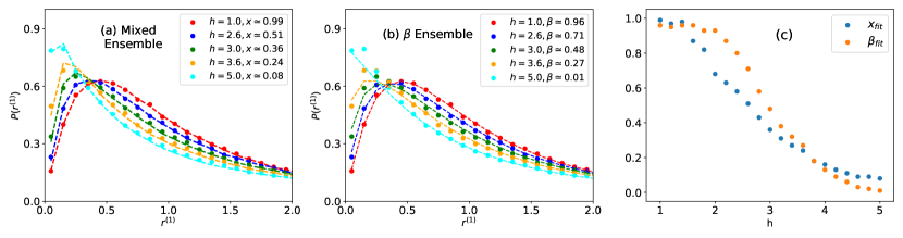
Figure 1: The fittings of $P\left(r^{(1)}\right)$ in orthogonal spin chain by (a) the mixed ensemble and (b) Gaussian $\beta$ ensemble, where the colored dots stand for numerical data of the physical Hamiltonian, and dotted lines stand for the optimized fitting results from RM models, the fitted model parameters are displayed in the figure legends. (c) Evolutions of the fitted parameters $x_{\text{fit}}$ and $\beta_{\text{fit}}$ along the thermal-MBL transition.

For the first step, we will show both the mixed ensemble and Gaussian $\beta$ ensemble can accurately reproduce $P\left(r^{\left(1\right)}\right)$ with properly chosen model parameters. These proper parameters are found by minimizing the following distance

$$D\left(\lambda\right)=\sum_{r}\left|P_{\text{mol}}\left(\lambda,r^{\left(1\right)}\right)-P_{\text{num}}\left(r^{\left(1\right)}\right)\right|^{2}\text{,}$$ (10)

where $P_{\text{mol}}\left(\lambda,r^{\left(1\right)}\right)$ is the target model distribution with parameter $\lambda$ standing for $x$ ($\beta$) in the mixed ensemble ($\beta$ ensemble), and $P_{\text{num}}\left(r^{\left(1\right)}\right)$ is the numerical data from physical model. For the latter, we simulate Eq. (9) in an $L=13$ system, with the Hilbert space dimension $N_{d}=2^{13}=8192$, and generate $400$ samples of eigenvalue spectrum at each disorder strengths. For each sample, we select $400$ eigenvalues in the middle to determine $P_{\text{num}}\left(r^{\left(1\right)}\right)$. We then determine the proper parameters by minimizing $D\left(\lambda\right)$, and draw the resulting $P_{\text{mol}}\left(r^{\left(1\right)}\right)$ together with $P_{\text{num}}\left(r^{\left(1\right)}\right)$, the results are collected in Fig. 1(a),(b).

As can be seen, both RM models reproduce $P_{\text{num}}\left(r^{\left(1\right)}\right)$ to a satisfying accuracy at all disorder strengths, even at the transition region. Generally, the mixed ensemble gives better performance than the $\beta$ ensemble, especially for cases with large disorder. This is because, when approaching the MBL phase, eigenvalue correlations become significantly short-ranged, while $\beta$ ensemble preserves level correlations on all ranges, which gives rise to larger deviations. These deviations will be more transparent when fitting higher-order spacing ratios.

To be complete, we draw the evolution of proper model parameters $x_{\text{fit}}$ and $\beta_{\text{fit}}$ with respect to the randomness strength $h\in\left[1,5\right]$ in Fig. 1(c). We observe monotonic decreasing tendencies for $x_{\text{fit}}$ and $\beta_{\text{fit}}$, both of which stand for decreasing level correlations, in consistent with physical intuition.

Now we proceed to study the longer-range level correlations through the higher-order spacing ratios $P\left(r^{\left(n\right)}\right)$ with $n>1$. To get an intuitive picture, we take the case with $h=3$ as a demonstration, which is at the critical region with largest fluctuations. The proper parameters can be read from Fig. 1(c), which is $x_{\text{fit}}=0.36$ for the mixed ensemble and $\beta_{\text{fit}}=0.48$ for the $\beta$ ensemble. We then draw the corresponding $P\left(r^{\left(2\right)}\right)$ and $P\left(r^{\left(3\right)}\right)$ of both models, and compare them to the physical data, the results are shown in Fig. 2. As we can see, both RM models show non-negligible deviations. More specifically, the peak of $P\left(r^{\left(2/3\right)}\right)$ in the $\beta$ ensemble is higher than the physical data, meaning it overestimates the longer-range level correlations, while the opposite is true for the mixed ensemble.

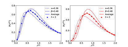
Figure 2: The fittings for the (left) 2nd-order spacing ratio $P\left(r^{\left(2\right)}\right)$ and (right) 3rd-order spacing ratio $P\left(r^{\left(3\right)}\right)$ for physical model with randomness strength $h=3$. The dotted and dashed lines correspond to the mixed ensemble and $\beta$ ensemble respectively, whose model parameters are determined by fitting $P\left(r^{\left(1\right)}\right)$, the solid lines are drawn by averaging the dotted and dashed lines.

Surprisingly, if we take a closer look at Fig. 2, we see the physical data lies roughly at the middle of the mixed ensemble and $\beta$ ensemble, which motivates us to draw the average of them, that is

$$P_{\text{ave}}\left(r^{\left(n\right)},x_{\text{fit}},\beta_{\text{fit}}\right)=\frac{P_{\text{mix}}\left(x_{\text{fit}}\text{,}r^{\left(n\right)}\right)+P_{\beta}\left(\beta_{\text{fit}}\text{,}r^{\left(n\right)}\right)}{2}\text{.}$$ (11)

The $P_{\text{ave}}\left(r^{\left(n\right)}\right)$ appear as the solid colored lines in Fig. 2, they match almost perfectly with the physical data, which indicates the deviations of two RM models cancel with each other. To confirm this is not a coincidence, we draw $P_{\text{ave}}\left(r^{\left(n\right)}\right)$ up to $n=7$ at various disorder strengths with corresponding proper parameters in Fig. 2(c), and compare them to the physical data, the results are collected in Fig. 3.

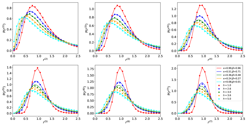
Figure 3: The fittings for higher-order spacing ratios at various disorder strengths, where the dots are numerical data, and lines are the average distribution $P_{\text{ave}}\left(r^{\left(n\right)}\right)$ according to Eq. (11), all figures share the same figure legends. Fairy good matches are found for $n\leq 4$, and the deviations starts to grow for $n\geq 5$ in the critical region($h\simeq 3$), reflecting the critical fluctuation in a finite system.

As can be seen, $P_{\text{ave}}\left(r^{\left(n\right)}\right)$ meets perfectly with the physical data up to $n=4$, that is, when $9$ consecutive levels are concerned, even at the critical region ($h\simeq 3$). The deviations starts to grow for $n>4$ at the critical region, which reflects the large critical fluctuations. These results suggest $P_{\text{ave}}\left(r^{\left(n\right)}\right)$ indeed gives an accurate account of the level evolutions along the thermal-MBL transition, which works not only for lowest-order level correlations, but also for correlations on moderate longer ranges.

Current results provide valuable indications about the evolution of level dynamics during MBL transition. First, results in Fig. 2 indicate the $\beta$ ensemble overestimates the long-range level correlations even it accurately captures the lowest-order one as shown in Fig. 1(b). This is not surprising since $\beta$ ensemble preserves level correlations on all ranges, while the level correlation becomes significantly short ranged when increasing disorder strength. Actually, such deviations have already appeared when fitting $P\left(r^{\left(1\right)}\right)$ deep in MBL phase in Fig. 1(b), which is further amplified when considering higher-order $P\left(r^{\left(n\right)}\right)$. This indicates only the interaction strength $\beta$ is not sufficient to cover the eigenvalue evolution during MBL transition, we must take interaction range into consideration. On the other hand, when studying the mixed ensemble, the interaction form, interaction range and strength all change when varying model parameter $x$, and results in a underestimation of long-range level correlations. This fact indicates not all the three aspects are responsible for MBL transition. Finally, an average of the two RM models gives proper description of level correlations along the MBL transition on moderate long ranges, which means the deviations in individual RM model cancel with the other one. Therefore, the only possible explanation is that the interaction between eigenvalues stays logarithmic while the interaction strength and range change during MBL transition, which in consistent with the $\beta-h$ model studied in Ref.[Sierant20, ]. However, as mentioned in the Introduction section, the $\beta-h$ model is built on eigenvalue distributions, while our model stems from two RM models with well-defined parent matrix construction.

The numerical results above are from an $L=13$ system, we have also confirmed that $P_{\text{ave}}\left(r^{\left(n\right)}\right)$ works fine for an $L=12$ system, although the fitted parameters $x_{\text{fit}}$ and $\beta_{\text{fit}}$ may have minor deviations, especially for cases in the transition region. We suspect these fitted parameters should converge when larger systems and more samples are considered, while the results from $L=13$ are sufficient to verify the efficiency of $P_{\text{ave}}\left(r^{\left(n\right)}\right)$.

At this stage, a working three-step strategy to reproduce the eigenvalue statistics at any disorder strength $h$ during thermal-MBL transition is proposed as follows. Step 1: Numerically compute the lowest-order spacing ratio distribution $P\left(r^{\left(1\right)}\right)$ of the physical Hamiltonian; Step 2: Find the proper parameter $x_{\text{fit}}$ (for the mixed ensemble) and $\beta_{\text{fit}}$ (for the $\beta$ ensemble) that fits best with $P\left(r^{\left(1\right)}\right)$, which is done by minimizing the distance $D\left(\lambda\right)$ in Eq. (10); Step 3: Compute the average distribution $P_{\text{ave}}\left(r^{\left(n\right)}\right)$ according to Eq. (11) with the proper parameters $x_{\text{fit}}$ and $\beta_{\text{fit}}$. The $P_{\text{ave}}\left(r^{\left(n\right)}\right)$ obtained in this manner is expected to faithfully describe level statistics along the thermal-MBL transition, even at critical region, at least when level correlations on moderate ranges are concerned. To further support this strategy, we proceed to consider MBL systems with unitary symmetry and quasi-periodic potential.

IV Unitary and Quasi-Periodic Systems

To consider a unitary system, we simulate Eq. (9) with $h_{x}=h_{y}=h_{z}=h$ in an $L=13$ system, with the rest technical settings identical to orthogonal case in previous section. This unitary model is known to exhibit a thermal-MBL transition at $h_{c}\simeq 2.5$, with corresponding RM description evolving from GUE to PoissonRegnault16 ; Regnault162 .

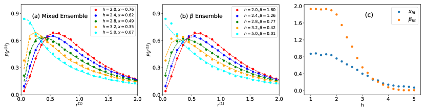
Figure 4: The fittings of $P\left(r^{\left(1\right)}\right)$ in the unitary spin model by (a) the mixed ensemble and (b) Gaussian $\beta$ ensemble. (c) Evolution of the fitted parameter $x_{\text{fit}}$ and $\beta_{\text{fit}}$ along the thermal-MBL transition.

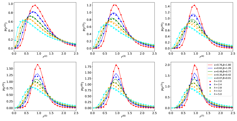
Figure 5: The fittings of higher-order spacing ratios at various disorder strengths in the unitary system, where the lines are the average distribution $P_{\text{ave}}\left(r^{\left(n\right)}\right)$. The fittings are close to perfect for $n\leq 3$, and starts to deviate for $n\geq 4$ for data in the critical region ($h\simeq 2.5$). The deviations are slightly lager than those in orthogonal system, reflecting larger critical fluctuations in finite system.

Like in the orthogonal case, we first show both the mixed ensemble and $\beta$ ensemble are capable of reproducing $P\left(r^{\left(1\right)}\right)$ with proper parameters $x_{\text{fit}}$ and $\beta_{\text{fit}}$ obtained by minimizing $D\left(\lambda\right)$ in Eq. (10). The fitting results are in Fig. 4(a),(b), note the parameter $\beta$ is ranging from $2$ (GUE) to $0$ (Poisson), and $x$ is now a parameter tuning the weight between GUE and Poisson. As expected, both RM models reproduce $P\left(r^{\left(1\right)}\right)$ quite well, even at the critical region. The evolution of $x_{\text{fit}}$ and $\beta_{\text{fit}}$ are drawn in Fig. 4(c), where expected decreasing tendencies are observed.

With the properly fitted parameters $x_{\text{fit}}$ and $\beta_{\text{fit}}$, we can determine $P_{\text{ave}}\left(r^{\left(n\right)}\right)$ according to Eq. (11) and compare them to the physical data at various disorder strengths, the results are collected in Fig. 5. As we can see, $P_{\text{ave}}\left(r^{\left(n\right)}\right)$ meets perfectly with physical data at all disorder strengths up to $n=3$, that is, when $7$ consecutive levels are considered. The deviations starts to grow for $n\geq 4$ in the transition region. Compared to the results in orthogonal model (perfect fittings for $n\leq 4$), the deviations are slightly larger, which reflects the critical fluctuations are larger in a unitary system.

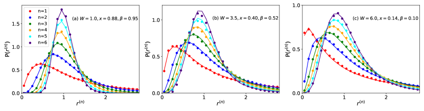
Figure 6: The comparison between $P_{\text{ave}}\left(r^{\left(n\right)}\right)$ got from Eq. (11) and physical data in the QP spin system in (a) thermal (W=1), (b) MBL (W=6) and (c) intermediate (W=3.5) region, where the optimized parameters $x$ and $\beta$ are obtained by fitting $P\left(r^{\left(1\right)}\right)$ with individual RM model. The fittings are even better than those in random disorder systems, whose qualitative explanations are in the main text.

Furthermore, we test this strategy in an MBL system induced by a different mechanism, that is, by quasi-periodic (QP) potential. The Hamiltonian is as follow

$$H_{\text{QP}} = J\sum_{i=1}^{L-1}\mathbf{s}_{i}\cdot\mathbf{s}_{i+1}+J^{\prime}\sum_{i=1}^{L-2}\left(s_{i}^{x}s_{i+2}^{x}+s_{i}^{y}s_{i+2}^{y}\right)$$ (12)

$$+W\sum_{\alpha=x,z}\sum_{i=1}^{L}\cos\left(2\pi ki+\varphi_{i}^{\alpha}\right)s_{i}^{\alpha}\text{,}$$

where $k=\frac{\sqrt{5}-1}{2}$(the Golden ratio), and $\varphi_{i}^{\alpha}\in\left(0,2\pi\right)$ is a random phase offset, the next-nearest neighbor term is introduced to break the integrability of clean system to stabilize the thermal phase. Without loss of generality, we choose $J=J^{\prime}=1$. Compared to models with random disorder, the potential in this model is incommensurate with lattice constant while deterministic, and hence is free of the Griffith regimeHuse3 . It is now widely-accepted the MBL transitions induced by random disorder and QP potential belong to different universality classes, although the values of critical exponents are under debateRD ; SXZhang .

For this QP model, we simulate three representative points in an $L=13$ system, that is, $W=1$ (thermal), $W=6$ (MBL) and $W=3.5$ (intermediate). At each point, we compare $P_{\text{ave}}\left(r^{\left(n\right)}\right)$ to physical data, the results are shown in Fig. 6. Perfect fittings for thermal/MBL phase are observed as expected. While for the intermediate region, fittings stays satisfying up to $n\leq 5$. Actually, comparing Fig. 6 to Fig. 3, we see $P_{\text{ave}}\left(r^{\left(n\right)}\right)$ works better for QP system than that with random disorder, which can be explained as follows.

From the viewpoint of eigenvalue statistics, MBL systems with QP potential and random disorder can be distinguished by the inter-sample randomnessRD ; Sierant19 . To be specific, we can determine the average spacing ratio in each sample of eigenvalue spectrum $r_{S}=\langle r\rangle_{\text{samp.}}$, then $P\left(r_{S}\right)$ – the distribution of $r_{S}$ over an ensemble of samples – will show deviations from a Gaussian distribution in system with random disorder, which reflects the existence of Griffiths regime. Consequently, $V_{S}$ – the variance of $r_{S}$ over ensemble – will exhibit a peak at the MBL transition point, while no such peak will appear in QP system. As we have checked, neither the mixed ensemble nor the $\beta$ ensemble can reproduce the peak of $V_{S}$ when varying their model parameters $x$ and $\beta$, therefore both of them are more optimal for QP systems, which may partially explain our observations.

V Conclusion and Discussion

We have proposed a working strategy to model the level statistics along the thermal-MBL transition in random spin systems.

Our strategy is based on two well-known random matrix (RM) models: the mixed ensemble and Gaussian $\beta$ ensemble. We showed both models can accurately reproduce $P\left(r^{\left(1\right)}\right)$ with properly chosen model parameters, while the fittings for higher-order spacing ratios have non-negligible deviations. Specifically, the mixed ensemble underestimates longer-range level correlations, while the opposite is true for $\beta$ ensemble. We further show these deviations strikingly cancel with each other by constructing their average $P_{\text{ave}}\left(r^{\left(n\right)}\right)$, which is capable of describing level correlation on moderate long ranges, even at the critical region. Our results suggest the interaction range and strength between eigenvalues are the two dominant features that responsible for the thermal-MBL transition, in consistent with conclusions of Ref.[Sierant20, ].

Our strategy has both pros and cons compared to the $\beta-h$ model of Ref.[Sierant20, ]. Although our strategy works fine for fitting $P\left(r^{\left(n\right)}\right)$ with $n<5$ in all cases, the deviations begin to be large for $n\geq 5$, which is outperformed by the $\beta-h$ model. However, one outstanding advantage of our strategy is that the two parameters $\left(x_{\text{fit}},\beta_{\text{fit}}\right)$ in the $P_{\text{ave}}\left(r^{\left(n\right)}\right)$ can be determined separately, that is, $x_{\text{fit}}(\beta_{\text{fit}})$ is obtained by fitting $P\left(r^{\left(1\right)}\right)$ with mixed ($\beta$) ensemble. While in $\beta-h$ model the two paramters have to be fitted jointly, which is much more difficult to implement.

Unlike the $\beta-h$ model, our strategy is based on two RM models that have well-defined parent matrix construction. It’s straightforward to ask what is the single random matrix model that corresponds to $P_{\text{ave}}\left(r^{\left(n\right)}\right)$. A natural guess would be the mixed version of mixed ensemble and $\beta$ ensemble, that is

$$M\left(x_{\text{fit}},\beta_{\text{fit}},y\right)=yM_{\alpha\rightarrow 0}\left(x_{\text{fit}}\right)+\left(1-y\right)M_{\beta_{\text{fit}}}\text{.}$$ (13)

However, our numerical attempts find no value of $y$ will reproduce the $P_{\text{ave}}\left(r^{\left(n\right)}\right)$, which indicates the average of spacing ratio distributions does not come from an linear combination of the random matrices. The final version of a single random matrix model remains to be explored.

Given the efficiency of $P_{\text{ave}}\left(r^{\left(n\right)}\right)$ around the critical region, it is hopeful that our strategy will be applicable when dealing with critical phenomena of MBL transition, especially in systems with quasi-periodic potential. There is a long debate on whether the MBL transition induced by random disorder and quasi-periodic potential bear identical critical exponent and hence belong to the same universality classRD ; SXZhang . Our strategy can contribute in this topic. A finite-size scaling study of the proper model parameters $x_{\text{fit}}$ and $\beta_{\text{fit}}$ around the transition region may help to determine the critical exponent of such a transition, which may suffer less from finite-size effect.

The physical systems studies in this work are mainly random spin chains, while it’s believed our strategy would work fine in other systems with characteristic level statistics evolutions. For example, the disordered Bose-Hubbard modelBose1 ; Bose2 , random quantum circuitsFriedman , interacting extended Harper modelHarper1 ; Harper2 , and so on.

Last but not least, it is interesting to ask if the statistics of entanglement spectrum can be modeled in the same way. Exploring this question will help to understand the relation between the statistics of eigenvalues to that of eigenstate wavefunction. These are all fascinating directions for future studies.

References

- (1) I. V. Gornyi, A. D. Mirlin, and D. G. Polyakov, Phys. Rev. Lett. 95, 206603 (2005); 95, 046404 (2005).
- (2) D. M. Basko, I. L. Aleiner, and B. L. Altshuler, Ann. Phys. 321, 1126 (2006).
- (3) J. M. Deutsch, Phys. Rev. A 43, 2046 (1991).
- (4) M. Srednicki, Phys. Rev. E 50, 888 (1994).
- (5) J. A. Kjall, J. H. Bardarson, and F. Pollmann, Phys. Rev. Lett. 113, 107204 (2014).
- (6) S. D. Geraedts, N. Regnault, and R. M. Nandkishore, New J. Phys. 19, 113921 (2017).
- (7) Z. C. Yang, C. Chamon, A. Hamma, and E. R. Mucciolo, Phys. Rev. Lett. 115, 267206 (2015).
- (8) M. Serbyn, A. A. Michailidis, M. A. Abanin, and Z. Papic, Phys. Rev. Lett. 117, 160601 (2016).
- (9) J. Gray, S. Bose, and A. Bayat, Phys. Rev. B 97, 201105 (2018).
- (10) M. Serbyn, Z. Papic, and D. A. Abanin, Phys. Rev. X 5, 041047 (2015).
- (11) H. Kim and D. A. Huse, Phys. Rev. Lett. 111, 127205 (2013).
- (12) J. H. Bardarson, F. Pollman, and J. E. Moore, Phys. Rev. Lett. 109, 017202 (2012).
- (13) M. Serbyn, Z. Papić, and D. A. Abanin, Phys. Rev. B 90, 174302 (2014).
- (14) V. Oganesyan and D. A. Huse, Phys. Rev. B 75, 155111 (2007).
- (15) Y. Avishai, J. Richert, and R. Berkovits, Phys. Rev. B 66, 052416 (2002).
- (16) N. Regnault and R. Nandkishore, Phys. Rev. B 93, 104203 (2016).
- (17) S. D. Geraedts, R. Nandkishore, and N. Regnault, Phys. Rev. B 93, 174202 (2016).
- (18) V. Oganesyan, A. Pal, D. A. Huse, Phys. Rev. B 80, 115104 (2009).
- (19) A. Pal, D. A. Huse, Phys. Rev. B 82, 174411 (2010).
- (20) S. Iyer, V. Oganesyan, G. Refael, D. A. Huse, Phys. Rev. B 87, 134202 (2013).
- (21) C. L. Bertrand and A. M. García-García, Phys. Rev. B 94, 144201 (2016).
- (22) D. J. Luitz, N. Laflorencie, and F. Alet, Phys. Rev. B 91, 081103(R) (2015).
- (23) M. L. Mehta, Random Matrix Theory, Springer, New York (1990).
- (24) F. Haake, Quantum Signatures of Chaos, (Springer 2001).
- (25) J. M. G. Gomez, R. A. Molina, A. Relano, and J. Retamosa, Phys. Rev. E 66, 036209 (2002).
- (26) P. Shukla, New J. Phys. 18, 021004 (2016).
- (27) M. Serbyn and J. E. Moore, Phys. Rev. B 93, 041424(R) (2016).
- (28) E. B. Bogomolny, U. Gerland and C. Schmit, Eur. Phys. J. B 19, 121 (2001).
- (29) X. Wei, R. Mondaini, and X. Gao, arXiv: 2001.04105.
- (30) W.-J. Rao, J. Phys. A: Math. Theor. 54, 105001 (2021).
- (31) P. Sierant and J. Zakrzewski, Phys. Rev. B 99, 104205 (2019).
- (32) W. Buijsman, V. Cheianov and V. Gritsev, Phys. Rev. Lett. 122, 180601 (2019).
- (33) P. Sierant and J. Zakrzewski, Phys. Rev. B 101, 104201 (2020).
- (34) P. Shukla, Phys. Rev. E 62, 2098 (2000).
- (35) P. Shukla, J. Phys.: Condens. Matter 17, 1653 (2005).
- (36) H. Kunz and B. Shapiro, Phys. Rev. E 58, 400 (1998).
- (37) V.E. Kravtsov, I. M. Khaymovich, E. Cuevas, and M. Amini, New J. Phys. 17, 122002 (2015)
- (38) Á. L. Corps, R. A. Molina, and A. Relaño, SciPost Phys. 10, 107 (2021).
- (39) S. Schierenberg, F. Bruckmann, and T. Wettig, Phys. Rev. E 85, 061130 (2012).
- (40) N. D. Chavda, H. N. Deota, and V. K. B. Kota, Phys. Lett. A 378, 3012 (2014).
- (41) Á. L. Corps and A. Relaño, Phys. Rev. E 101, 022222 (2020).
- (42) I. Dumitriu and A. Edelman, J. Math. Phys. (N.Y.) 43, 5830 (2002).
- (43) Y. Y. Atas, E. Bogomolny, O. Giraud, and G. Roux, Phys. Rev. Lett. 110, 084101 (2013).
- (44) S. H. Tekur, U. T. Bhosale, and M. S. Santhanam, Phys. Rev. B 98, 104305 (2018).
- (45) W.-J. Rao, Phys. Rev. B 102, 054202 (2020).
- (46) W.-J. Rao and M. N. Chen, Eur. Phys. J. Plus 136, 81 (2021).
- (47) F. Alet and N. Laflorencie, C. R. Physique 19, 498-525 (2018).
- (48) V. Khemani, D. N. Sheng, and D. A. Huse, Phys. Rev. Lett. 119, 075702 (2017).
- (49) S.-X. Zhang and H. Yao, Phys. Rev. Lett. 121, 206601 (2018).
- (50) P. Sierant, D. Delande, and J. Zakrzewski, Phys. Rev. A 95, 021601 (2017).
- (51) P. Sierant and J. Zakrzewski, New J. Phys. 20, 043032 (2018).
- (52) A. J. Friedman, A. Chan, A. De Luca, J. T. Chalker, Phys. Rev. Lett. 123, 210603 (2019).
- (53) Y. Wang, C. Cheng, X.-J. Liu, and D. Yu, Phys. Rev. Lett. 126, 080602 (2021).
- (54) Y. Takada, K. Ino, and M. Yamanaka, Phys. Rev. E 70, 066203 (2004).