Markovian online matching algorithms on large bipartite random graphs

Abstract.

In this paper, we present an approximation of the matching coverage on large bipartite graphs, for local online matching algorithms based on the sole knowledge of the remaining degree of the nodes of the graph at hand. This approximation is obtained by applying the Differential Equation Method to a measure-valued process representing an alternative construction, in which the matching and the graph are constructed simultaneously, by a uniform pairing leading to a realization of the bipartite Configuration Model. The latter auxiliary construction is shown to be equivalent in distribution to the original one. It allows to drastically reduce the complexity of the problem, in that the resulting matching coverage can be written as a simple function of the final value of the process, and in turn, approximated by a simple function of the solution of a system of ODE’s. By way of simulations, we illustrate the accuracy of our estimate, and then compare the performance of an algorithm based on the minimal residual degree of the nodes, to the classical greedy matching.

1. Introduction

Maximal matching on graphs is a classical problem in graph theory. Its applications range from simple scheduling to online advertisement, from jobs or housing allocations to the sequencing of protein chains, and so on. Long after the first polynomial optimal solution, proposed by Edmonds [16], this problem has still received a significant attention, especially over the last three decades, due to the rise of large networks, leading to a flourish of new applications (in e-commerce, for example), forcing a reexamination of the tools previously used. As a consequence, two main new approaches emerged.

In 1990, Karp et al. [23] introduced the concept of Online bipartite matching. In this paradigm, the graph is split into customers and items. Customers arrive one by one, and it is the role of the matching algorithm to pick one of the items for a match. These assumptions lead to a natural tradeoff between optimality in the matching size and cheaper costs. In [23], Karp et al. used the adversarial order of arrivals as a worst case scenario for the matching completion, leading to the now classical $1-1/e$ bound for the matching coverage, namely, the ratio of matched items out of the total set. This ratio is achieved whenever the nodes are drawn repeatedly from a known distribution, and the matching algorithm is greedy - see below. The construction of algorithms that are able to beat this benchmark under various conditions, has then been the subject of an important line of research, see e.g. [20, 18] and references therein. More recently, various extensions of the online bipartite matching problem have been proposed among which, stochastic matching [6] (meaning that each edge emanating from the online nodes exists with a given probability), random customer arrivals [25], or models with patience times [9]. Bounds for matching algorithms on (general) random regular graphs of fixed girth are given in [19], using a randomized version of the greedy matching algorithm.

The second approach is more typically computer-scientific. Streaming algorithms are algorithms that only process a stream, on a limited part of a given graph (for memory constraints for example). They arise as a natural solution while dealing with large data sets and several authors have worked to apply them to the matching problem (see e.g. [10], [17] and [28], and references therein). This line of research mainly addressed the type of input for the stream (either dynamic or enter only), its randomness or its relative size to the whole graph.

Most references above provide bounds for the performance of given algorithms, that are supported by combinatorial arguments. However, precisely assessing the performance of a given matching algorithm as the size of the graphs gets large, is a challenging problem. Indeed, the analysis of the asymptotic of a sequence of graphs, and matchings on those graphs becomes less and less tractable as their size grows large. It can then be preferable to approximate the matching size as a function of a scalable statistic of the graph. Following this line of thought, in this paper we propose an alternative approach to the bipartite matching problem: assessing the performance of given matching algorithms through a deterministic approximation of a stochastic process representing the matching procedure, in the large graph asymptotic. The general idea is as follows: rather than precisely defining and keeping track of the whole geometry of the graph (an information that is in general unavailable for large graphs), we generate a graph from its degree distribution. To this end, we use a classical uniform pairing procedure of the half-edges of the nodes, see a precise definition below. This construction leads to the so-called Configuration model, namely, a uniformly drawn realization of a graph having the prescribed degree distribution. See [5] and [22] for the main properties of configuration models, and [11] for the extension to the case of bipartite and oriented graphs. In parallel, we construct simultaneously an online matching (meaning in this context, that each edge that is added to the matching cannot be erased afterwards) on the resulting graph. As a main interest, this simultaneous construction leads to a simple Markov representation, keeping track of the remaining degrees of the nodes that are not yet fully attached to the graph (a definition that will be made precise hereafter), provided that the matching algorithm depends only on these remaining degrees. We say in that case that the matching algorithm is local. The underlying Markov process is then measure-valued, where each measure is a sum of Dirac masses marking the remaining degrees of the nodes. By doing so, we do not need to keep track of the precise form of the constructed graph, and in fact, we do not need to have access to it. Then, using usual approximation tools for Markov processes, one can identify the approximation of the considered process as the solution of an ordinary differential equation. This results in a generalization, for measure-valued processes, of the celebrated Differential Equation Method, see Wormald [29]. By doing so, we retrieve an estimate of the resulting matching coverage as a simple function of the latter (deterministic) solution, without knowledge of the precise geometry of the graph at hand. Remarkably, we show hereafter that the resulting matching coverage has the same distribution as the one obtained when applying the corresponding online, and local, matching algorithm on a previously constructed bipartite graph $\tilde{G}$, conditional on the fact that the resulting graph constructed by the CM is precisely $\tilde{G}$. As a consequence, our estimate of the matching coverage by the differential equation method, provides a remarkably accurate estimation of the matching coverage of the considered local algorithm on a given bipartite graph, a result that we support with extensive simulations.

The extension of the differential equation method to measure-valued processes, resulting from a simultaneous construction of the CM and an exploration algorithm on the latter, first appeared in [12], to describe the propagation of an SIR epidemics on an heterogenous graph. Then a closely related idea was applied in [3], to approximate the size of maximal independent sets on graphs with given degree distributions (for a more direct use of the differential equation method on the same topic, see also [7]). This led to various extensions, to address various coverage problems in CSMA-type algorithms for radio-mobile and ad-hoc communication networks, see [1].

Before that, measure-valued processes Markov processes were first introduced in the queueing literature. Space of measures are amenable to showing weak convergence of sequence of processes under an appropriate scaling, and the exhaustive representation of queueing systems by point measures, in which each Dirac mass typically represents the characteristic of a customer in line, led to fruitful developments in fluid and diffusion approximations of the systems at hand, see e.g. [21] for processor sharing queues, [15, 13] for queueing systems with impatient customers, [14] for infinite-server queues, or [24] for many-server queues.

This paper is organized as follows. After a preliminary section, in Section 3 we define the local matching algorithms we will address hereafter, among which, the minimal residual algorithm, which can be seen as an analog of the Degree-greedy algorithm defined in [2] for the construction of maximal independent sets on random graphs. In Section 4, we detail our joint construction of a random (multi-)graph by the CM, and of an online matching on the latter. As will clearly appear below, the local matching algorithms then work as some kind of tagging processes, alongside the uniform-pairing construction process of the configuration model. In Section 5, we introduce the measure-valued Markov processes representing the two previous constructions. In particular, Theorem 1 presents a simple connexion between the two processes. In Section 6, we introduce our hydrodynamic approximation, namely, the limiting system of Ordinary Differential Equations approximating the dynamics of the measure-valued process representing the construction of Section 4. Finally, in Section 7 we present our simulation results. We first illustrate the accuracy of our approximation for various degree distributions, and then compare the matching coverage obtained by the minimal residual algorithm to that resulting from the greedy algorithm. We also briefly compare our results with the results of Karp et al. in [23]. All our code and data are available upon request.

2. Preliminary

We denote respectively by ${\mathbb{R}}$, ${\mathbb{R}}_{+}$, ${\mathbb{N}}$ and ${\mathbb{N}}^{*}$, the sets of real numbers, non-negative real numbers, of non-negative and positive integers. For any finite set $A$, we write $|A|$ for the cardinality of $A$. For any $a\leq b\in{\mathbb{N}}$, we let $\llbracket a,b\rrbracket$ denote the integer interval $\{a,a+1,...,b-1,b\}$. We let ${\mathcal{M}}({\mathbb{N}})$ be the set of integer finite measures on ${\mathbb{N}}$. Denote for any $\mu$ in ${\mathcal{M}}({\mathbb{N}})$ and any $\varphi:{\mathbb{R}}\to{\mathbb{R}}$ such that the following is well defined,

$$\left\langle\mu,\varphi\right\rangle=\int_{{\mathbb{N}}}\varphi(x)\text{ d}\mu(x)=\sum_{i\in{\mathbb{N}}}\varphi(i)\mu(i).$$

Let $\mathcal{B}_{b}({\mathbb{N}})$ be the space of bounded functions: ${\mathbb{N}}\to{\mathbb{R}}$. We denote by $\mathbf{1}$, the function ${\mathbb{R}}\to{\mathbb{R}}$ that is identically equal to 1, $X$ the identity function on ${\mathbb{R}}$ and $X^{2}(x)=x^{2}$ for all $x\in{\mathbb{R}}$. As a consequence, for any $\mu\in{\mathcal{M}}({\mathbb{N}})$, $\left\langle\mu,\mathbf{1}\right\rangle$, $\left\langle\mu,X\right\rangle$ and $\left\langle\mu,X^{2}\right\rangle$ denote respectively the total mass, the first and the second moment of $\mu$, if any. Denote also for all $\varphi:{\mathbb{N}}\to{\mathbb{R}}$, by $\Delta\varphi$ the discrete gradient of $\varphi$, defined by

$$\Delta\varphi(x)=\varphi(x)-\varphi(x-1),\,x\in{\mathbb{N}}.$$

All random variable are defined on a common probability space $(\Omega,\mathcal{F},{\mathbb{P}})$. The space ${\mathcal{M}}({\mathbb{N}})$ is endowed with its weak topology, in other words $\mu^{n}\longrightarrow\mu$ in ${\mathcal{M}}({\mathbb{N}})$ whenever $\left\langle\mu^{n},\varphi\right\rangle\longrightarrow\left\langle\mu,\varphi\right\rangle$ for all bounded $\varphi$. Then it is well known that ${\mathcal{M}}({\mathbb{N}})$ is a Polish space, see e.g. [4].

For any Polish space $E$, we denote by $\mathrm{D}([0,1],E)$ the space of cadlag (i.e. right-continuous, with left-hand limits at all points) $E$-valued processes on $[0,1]$, equipped with the Skorokhod topology.

3. Local matching algorithms on a graph

We start by introducing the general class of matching algorithms we will consider hereafter.

3.1. Matching through exploration on a graph

We now define the class of local matching algorithms we consider in this work, in a sense to be specified below. We fix a (non-oriented) bipartite graph $G=(V,E)$, where $V=V^{+}\cup V^{-}$ is the set of nodes and $E\subset V^{+}\times V^{-}$ is the set of edges. We assume that the bipartition of the graph is balanced, i.e., $|V^{+}|=|V^{-}|=n$ for some positive integer $n$. At any time $t$, we are given two disjoint subgraphs of $G$:

• $\tilde{G}_{t}=(\tilde{U}_{t},\tilde{E}_{t})$ represents the remaining graph of our construction at $t$. The nodes of $\tilde{U}_{t}$ are said undetermined at $t$. As will appear clearly in the construction below, the graph $\tilde{G}_{t}$ is itself bipartite (as a subgraph of a bipartite graph), and we denote by $\tilde{U}_{t}=\tilde{U}_{t}^{+}\cup\tilde{U}^{-}_{t}$, the bipartition of its nodes. For any $\tilde{v}\in\tilde{U}_{t}$ we denote by $N_{t}(\tilde{v})$ the set of neighbors of $\tilde{v}$ at $t$, and by $d_{t}(\tilde{v})=|N_{t}(\tilde{v})|$ the degree of $\tilde{v}$ at $t$, namely, the number of its neighbors in $\tilde{G}_{t}$.

• $\tilde{G}^{\prime}_{t}=(\tilde{M}_{t},\tilde{E}^{\prime}_{t})$ is the matching at time $t$. This is also a (bipartite) subgraph of $G$ in which all nodes are of degree one. The set $\tilde{M}_{t}:=\tilde{M}^{+}_{t}\cup\tilde{M}^{-}_{t}$ gathers the matched nodes at $t$.

We also let $\tilde{I}_{t}$ be the set of isolated nodes at $t$. These are nodes that won’t appear in the final matching, and we have the disjoint union $V=\tilde{U}_{t}\cup\tilde{M}_{t}\cup\tilde{I}_{t}$.

At first, all nodes are undetermined, i.e. we set $\tilde{U}_{0}=V$, $\tilde{M}_{0}=\emptyset$ and $\tilde{I}_{0}=\emptyset$. We also set $\tilde{E}_{0}=E$ and $\tilde{E}^{\prime}_{0}=\emptyset$, in a way that $\tilde{G}_{0}=G$ and $\tilde{G}^{\prime}_{0}=(\emptyset,\emptyset)$. The matching algorithm then proceeds by induction, as follows: At any time $t\in\llbracket 0,n-1\rrbracket$,

1. A vertex $\tilde{J}^{+}$ is chosen uniformly at random in $\tilde{U}^{+}_{t}$.

   Figure 1. Exploring a vertex of a bipartite graph

2. We select a match for $\tilde{J}^{+}$ if this is feasible at all:

   1. If $\tilde{J}^{+}$ has at least one neighbor in $\tilde{U}_{t}^{-}$, i.e., if the set $N_{t}(\tilde{J}^{+})$ is non-empty, then it is the role of the matching criterion to select one of these, say $\tilde{J}^{-}$, to be the match of $\tilde{J}^{+}$. We assume that the criterion is local in the sense that it only depends on the degrees of the neighbors of $\tilde{J}^{+}$, and possibly on a random choice that is independent of every other random variables so far. To formalize this, fix a deterministic mapping

      (1) $$\Phi:\begin{cases}\displaystyle\bigcup_{k=1}^{n}\,({\mathbb{N}}^{*})^{k}&\longrightarrow\llbracket 1,n\rrbracket\\ \displaystyle(x_{1},...,x_{k})&\longmapsto j\in\llbracket 1,k\rrbracket\end{cases}.$$

      Then, let $k:=|N_{t}(\tilde{J}^{+})|\leq|\tilde{U}^{-}_{t}|$, denote by $\left\{\tilde{J}^{-}_{1},...,\tilde{J}^{-}_{k}\right\}$, the elements of $N_{t}(\tilde{J}^{+})$, and draw a permutation $\sigma\in\mathfrak{S}_{k}$ uniformly at random. The permutation $\sigma$ is possibly used to draw a list of priorities between elements of $N_{t}(\tilde{J}^{+})$. Then, we set $\tilde{J}^{-}:=\Phi(\tilde{J}^{+}):=\tilde{J}^{-}_{\sigma(j)}$, where $j=\Phi\left(d_{t}(\tilde{J}^{-}_{\sigma(1)}),...,d_{t}(\tilde{J}^{-}_{\sigma(k)})\right)$. In Figure 2, the match is represented in blue for two examples of local matching criteria: greedy and minres, properly defined in Definition 1.

      

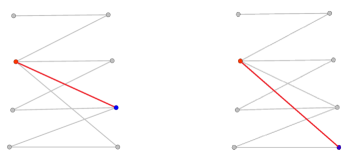
      Figure 2. Selecting the match for the two algorithms greedy (left) and minres (right), defined in Definition 1.

      Then the matched nodes $\tilde{J}^{+}$ and $\tilde{J}^{-}$ are deleted from the graph $\tilde{G}_{t}$, and added to the matching $\tilde{G}^{\prime}_{t}$. Specifically, we set

      $$\left\{\begin{array}[]{lll}\tilde{U}_{t+1}&=\tilde{U}_{t}\setminus\{\tilde{J}^{+},\tilde{J}^{-}\},&\tilde{G}_{t+1}=\mbox{Induced subgraph of }\tilde{U}_{t+1}\mbox{ in }\tilde{G}_{t},\\ \tilde{M}_{t+1}&=\tilde{M}_{t}\cup\{\tilde{J}^{+},\tilde{J}^{-}\},&\tilde{E}^{\prime}_{t+1}=\tilde{E}_{t}\cup\{\{\tilde{J}^{+},\tilde{J}^{-}\}\},\\ \tilde{I}_{t+1}&=\tilde{I}_{t}.&\end{array}\right.$$

      Figure 3 shows the resulting graph $\tilde{G}_{t+1}$.

      

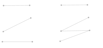
      Figure 3. Resulting graph $\tilde{G}_{t+1}$ after the deletion of the matched vertices, for greedy (left) and minres (right)

      .

   2. If $\tilde{J}^{+}$ has no neighbor in $\tilde{U}_{t}^{-}$, i.e., $N_{t}(\tilde{J}^{+})=\emptyset$, then $\tilde{J}^{+}$ is just added to the set of isolated nodes, i.e. we set

      $$\tilde{U}_{t+1}=\tilde{U}_{t},\quad\tilde{E}_{t+1}=\tilde{E}_{t},\quad\tilde{M}_{t+1}=\tilde{M}_{t},\quad\tilde{E}^{\prime}_{t+1}=\tilde{E}_{t},\quad\tilde{I}^{+}_{t+1}=\tilde{I}^{+}_{t}\cup\{\tilde{I}^{+}\}.$$

3. We set $t:=t+1$ and go back to step 1.

At the terminating point $t=n$ of the procedure, we necessarily get that $|\tilde{M}^{+}_{n}|=|\tilde{M}^{-}_{n}|$ and $\tilde{U}^{+}_{n}=\emptyset$. Notice that, if $|\tilde{I}^{+}_{n}|\neq 0$, then there are at time $n$, as many undetermined nodes on the right-hand side as of isolated nodes on the left-hand side, namely there are $|\tilde{I}^{+}_{n}|$ of them. We can then set all undetermined nodes on the right-hand side as isolated, since the latter nodes can no longer be attached to the matching, i.e. we set $\tilde{I}^{-}_{n}:=\tilde{U}^{-}_{n}$, and then $\tilde{U}^{-}_{n}:=\emptyset$. We finally obtain that

$$|\tilde{M}_{n}|+|\tilde{I}_{n}|=2n,$$

in other words all nodes are either matched, or isolated. The matching coverage $\tilde{\mathbf{M}}^{n}_{\Phi}(G)$ is then the proportion of initial nodes that ended up in the matching at the termination time $n$, that is,

(2) $$\tilde{\mathbf{M}}^{n}_{\Phi}(G)={|\tilde{M}_{n}|\over 2n}=1-{|\tilde{I}_{n}|\over 2n}\,\,\in[0,1].$$

We now define two particular local matching algorithms,

Definition 1.

• We say that $\Phi$ is greedy, and we denote $\Phi=\textsc{greedy}$ if, at step 3a) above $\tilde{J}^{-}$ is chosen uniformly at random, independently of all r.v.’s involved up to $t$, within the set $N_{t}(\tilde{J}^{+})$. Specifically, in (1) we set $\Phi(x_{1},...,x_{k})=1$ for any $k\in\llbracket 1,n\rrbracket$ and all $(x_{1},...,x_{k})\in({\mathbb{N}}^{*})^{k}$, in a way that $\tilde{J}^{-}=\tilde{v}_{\sigma(1)}$. In other words, the permutation $\sigma$ is used to draw, uniformly at random, a list of priorities between the elements of $N_{t}(\tilde{J}^{+})$, and the priority node $\tilde{v}_{\sigma(1)}$ is chosen as the match of $\tilde{J}^{+}$.

• We say that $\Phi$ is minimal residual, and we denote $\Phi=\textsc{minres}$ if, at step 3a) above, we chose $\tilde{J}^{-}$ uniformly at random, independently of all r.v.’s up to $t$, within the set of nodes of minimal residual degree in $\tilde{G}_{t}$ amongst the neighbors of $\tilde{J}^{+}$. Then, we use again $\sigma$ to construct a list of priorities between the nodes of minimal degree in $\tilde{U}^{-}_{t}$, and in (1) we set

  $$\Phi(x_{1},...,x_{k})=\min\Bigl{\{}\ell\in\llbracket 1,k\rrbracket\,:\,\ell\in\mbox{argmin}\left\{x_{i}\,:\,i\in\llbracket 1,k\rrbracket\right\}\Bigl{\}}$$

  for all $k$ and all $(x_{1},...,x_{k})\in({\mathbb{N}}^{*})^{k}$.

Remark 1.

A similar algorithm, called Degree-greedy, was proposed in [2] for constructing maximal independent sets on general graphs.

Algorithm 1 General local matching algorithm for a choice criterion $\Phi$

0:  Non-empty bipartite graph $G(V^{+}\cup V^{-},E)$

  $\mbox{Matching}\leftarrow\emptyset$;

  for $t<n$ do

     Pick a (uniformly) random vertice $\tilde{J}^{+}$ in $\tilde{U}^{+}$;

     Discover its neighborhood $N(\tilde{J}^{+})$ in $\tilde{U}^{-}$;

     $\tilde{U}^{+}\leftarrow\tilde{U}^{+}\setminus\left\{\tilde{J}^{+}\right\}$;

     if $N(\tilde{J}^{+})$ is empty then

        Do not do anything more

     else

        $\tilde{J}^{-}\leftarrow\Phi(\tilde{J}^{+})$;

        $\tilde{U}^{-}\leftarrow\tilde{U}^{-}\setminus\left\{\tilde{J}^{-}\right\}$;

        $\mbox{Matching}\leftarrow\mbox{Matching}\cup(\tilde{J}^{+},\tilde{J}^{-})$;

     end if$t\leftarrow t+1$;

  end for

4. Coupled construction with the Configuration Model

The previous matching algorithms are based on an exploration of the bipartite graph under consideration. By their inductive construction, as defined above, they naturally induce a Markovian dynamics. However, throughout the construction, one needs to keep track of the whole topology of the graph. As the size of the graph grows large, this approach has two main limitations: First, it leads to a dramatic increase of the size of the state space of the underlying Markov process - see below. Second, in practical cases, one rarely has access to the whole topology of a large network. Instead, a more restricted statistical information can be made available, such as the distribution of the degrees (i.e. the size of the neighborhoods) of the nodes.

To address both difficulties at once, in this section we show how to assess the performance of the algorithms under consideration, by introducing a Markovian construction based solely on the degree distribution of the nodes, without any knowledge of the precise topology of the graph. For doing so, one way is to generate uniformly at random, a graph having a prescribed degree distribution, and to perform simultaneously the matching algorithm under consideration, as described in Section 3.

As is well known, a uniform random realization of a graph having a given degree distribution can be obtained via the uniform pairing procedure, inherent to the so-called Configuration Model (CM, for short), see [5, 26]. This procedure consists of initially considering that all nodes are detached from the graph, and have as many half-edges as their degree, and then to selecting sequentially, uniformly at random, nodes, and attaching to the graph by pairing their half-edges to other ones, chosen again uniformly at random. It is easily seen that such a procedure in general leads to a multi-graph, i.e. a graph containing self-loops and/or multiple edges; however the number of such “bad” edges can be shown to be a $o(1/n)$, or even less [27], see e.g. [22] for the CM on general graph, and [11] for CM on bipartite and oriented graphs.

In this section, the dynamics of the analog of the local algorithms defined in Section 3 are constructed simulatenously with the configuration model. This joint construction will induce a more simple Markovian dynamics, leading in turn to a simple approximation of the matching coverage of the model, see Section 6.

4.1. Local matching algorithms on the CM

Let $\xi^{+}$ and $\xi^{-}$ be two probability measures on ${\mathbb{N}}$. Let $n$ be a positive integer and $\mathbf{d}^{+}:=(d^{+}(1),...,d^{+}(n))$ and $\mathbf{d}^{-}:=(d^{-}(1),...,d^{-}(n))$ be two $n$-samples, respectively of the probability distributions $\xi^{+}$ and $\xi^{-}$. These two samples are conditioned to have the same total mass, i.e., to be such that $\sum_{i=1}^{n}d^{+}(i)=\sum_{i=1}^{n}d^{-}(i).$ Their elements will hereafter represent the degrees of the nodes on both sides of the bipartition, see e.g. Figure 4 for $n=4$.

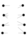
Figure 4. A running example : $\hat{\mu}_{0}^{+}=2\delta_{1}+\delta_{2}+\delta_{4}$ and $\hat{\mu}_{0}^{-}=4\delta_{2}$

We now introduce our joint construction of a multi-graph having degree distributions $\mathbf{d}^{+}$ and $\mathbf{d}^{-}$, and of a matching on the latter. We let $V^{+}=\{v_{1}^{+},...,v_{n}^{+}\}$ (resp., $V^{-}=\{v_{1}^{-},...,v_{n}^{-}\}$) be the set of nodes of the graph on the left-hand (resp., right-hand) side of the bipartition, and view for all $i\in\llbracket 1,n\rrbracket$, $d^{+}(i)$ (resp., $d^{-}(i)$) as the degree of node $v_{i}^{+}$ (resp. $v_{i}^{-}$). We then set for all $i$, $a_{0}(v^{+}_{i})=d^{+}(i)$ and $a_{0}(v^{-}_{i})=d^{-}(i)$, and define the two following sets,

$$A^{+}_{0}=\Bigl{\{}\bigl{(}v^{+}_{1},a_{0}(v^{+}_{1})\bigl{)},\cdots,\bigl{(}v^{+}_{n},a_{0}(n)\bigl{)}\Bigl{\}},\quad A^{-}_{0}=\Bigl{\{}\bigl{(}v^{-}_{1},a_{0}(v^{-}_{1})\bigl{)},\cdots,\bigl{(}v^{-}_{n},a_{0}(v^{-}_{n})\bigl{)}\Bigl{\}}.$$

Observe that we have $\sum_{l=1}^{n}a_{0}(v^{+}_{i_{l}})=\sum_{l=1}^{p}a_{0}(v^{-}_{j_{l}})$ by assumption. At first, the graph $G_{0}$ consists of the set of disconnected nodes $V:=V^{+}\cup V^{-}$, i.e., $G_{0}=(V,\emptyset)$. We also set $M_{0}^{+}=M_{0}^{-}=\emptyset$, $U_{0}^{+}=V^{+}$ and $U^{-}_{0}=V^{-}$, and let $G^{\prime}_{0}$ be the empty graph, i.e. $G^{\prime}_{0}=(\emptyset,\emptyset)$. We then proceed by induction, as follows. At any time $t$, we are given:

• A bipartite multi-graph $G_{t}=(V,E_{t})=(M_{t}\cup U_{t}\cup I_{t},E_{t})$ representing the partially constructed connexions between elements of $V$, where we denote by :

  • $M_{t}^{+}$ (resp., $M_{t}^{-}$) the set of matched nodes at $t$ on the left-hand (resp., right-hand) side at $t$, which are nodes that are fully attached to the graph at $t$, and belong to the matching at $t$;

  • $U_{t}^{+}$ (resp., $U_{t}^{-}$), the set of undetermined nodes at $t$ on the left-hand (resp., right-hand) side, that is, nodes that do not belong to the matching at $t$, but can still be attached to it;

  • $I_{t}^{+}$, the set of isolated nodes at $t$ on the left-hand side, that is, nodes that are already fully attached to the graph at $t$, but do not belong to the matching at $t$.

  We also set $M_{t}=M^{+}_{t}\cup M^{-}_{t}$ and $U_{t}=U^{+}_{t}\cup U^{-}_{t}$. By our very construction, all nodes of $M_{t}$ (if any) will have degree at least one in $G_{t}$, and we let $U^{+}_{t}=\{v^{+}_{i_{1}},...,v^{+}_{i_{p}}\}\subset V^{+}$ and $U^{-}_{t}=\{v^{-}_{j_{1}},...,v^{-}_{j_{r}}\}\subset V^{-}$. (We skip the dependance in $t$ in the parameters $v^{+/-}_{j_{l}}$, for short.)

• A perfect matching $G^{\prime}_{t}=(M_{t},E^{\prime}_{t})$ on the induced subgraph of $M_{t}$ in $G_{t}$. In particular, $E^{\prime}_{t}$ is a set of subsets of pairs of $M_{t}$ of the form $\{v^{+}_{i},v^{-}_{j}\}$ for $v_{i}^{+}\in M^{+}_{t}$ and $v_{j}^{-}\in M_{t}^{-}$, such that any element of $M_{t}$ appears in exactly one pair of $E^{\prime}_{t}$.

• A couple of sets of pairs

  $$A^{+}_{t}=\Bigl{\{}\bigl{(}v^{+}_{i_{1}},a_{t}(v^{+}_{i_{1}})\bigl{)},\cdots,\bigl{(}v^{+}_{i_{p}},a_{t}(v^{+}_{i_{p}})\bigl{)}\Bigl{\}},\quad A^{-}_{t}=\Bigl{\{}\bigl{(}v^{-}_{j_{1}},a_{t}(v^{-}_{j_{1}})\bigl{)},\cdots,\bigl{(}v^{-}_{j_{n}},a_{t}(v^{-}_{j_{n}})\bigl{)}\Bigl{\}},$$

  such that $\sum_{l=1}^{n}a_{t}(v^{+}_{i_{l}})=\sum_{l=1}^{p}a_{t}(v^{-}_{j_{l}})$ (possibly understanding sums over empty sets as 0). For any $l\in\llbracket 1,p\rrbracket$ we interpret $a_{t}(v^{+}_{i_{l}})$ as the availability of node $v^{+}_{i_{l}}$ at $t$, that is, the number of available half-edges (towards the right-hand side) of $v^{+}_{i_{l}}$, and likewise for the right-hand side. See an example on Figure 5.

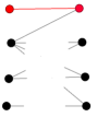
Figure 5. State at iteration $t$ : the matched nodes (elements of $G^{\prime}_{t}$) are red. The undetermined nodes (labelled from top to bottom) are black, and we get $A_{t}^{+}=\left\{(v^{+}_{i_{1}},3),(v^{+}_{i_{2}},2),(v^{+}_{i_{3}},1)\right\}$; $A_{t}^{-}=\left\{(v^{-}_{j_{1}},2),(v^{-}_{j_{2}},2),(v^{-}_{j_{3}},2)\right\}$.

Then we proceed as follows: at any time $t\in\llbracket 0,n-1\rrbracket$,

1. We select an uncompleted node on the left-hand uniformly at random, and then complete its neighborhood in the graph. Specifically, we first draw the realization of a r.v. of uniform distribution $\mathscr{U}\left(\llbracket 1,p\rrbracket\right)$. Say the outcome is $q$. Then, we set $J^{+}=v^{+}_{i_{q}}$, see Figure 6.

   

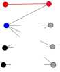
   Figure 6. $J^{+}$ chosen at iteration t

   We then complete the $a_{t}\left(J^{+}\right)$ half-edges of $J^{+}$, if any, into edges by joining them to half edges picked uniformly at random among the half-edges on the right-hand side. Specifically,

   1. If $a_{t}(J^{+})>0$, we draw $a_{t}\left(J^{+}\right)$ elements uniformly at random among $n$ “bunches” of elements of respective sizes $a_{t}\left(v^{-}_{j_{l}}\right)$, $l\in\llbracket 1,n\rrbracket$, to construct the emanating edges of node $J^{+}$ toward the ‘-’ side, and thereby, its neighbors on the opposite side. We let $\{J^{-}_{1},...,J^{-}_{k}\}\subset\left\{v^{-}_{j_{1}},...,v^{-}_{j_{n}}\right\}$, where $k\leq a_{t}\left(J^{+}\right)$, be the set of the $k$ neighbors of $J^{+}$, i.e., the indexes of the bunches containing the chosen half-edges. Note that this operation may lead to multiple edges, whenever several elements of the same bunch of half-edges are chosen, and in this case we have $k<a_{t}\left(J^{+}\right)$. For all $l\in\llbracket 1,k\rrbracket$, we let $E^{-}_{l}$ be the number of edges shared by $J^{-}_{l}$ with $J^{+}$, that is, the number of elements in the bunch $J^{-}_{l}$ chosen in the uniform pairing procedure. Then the neighborhood of $J^{+}$ is completed, see Figure 7.

      

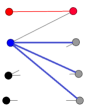
      Figure 7. The neighbors of $J^{+}$ are discovered.

   2. If $a_{t}(J^{+})=0$, then node $J^{+}$ has no available half-edge at this point. Its neighborhood in the graph has thus already been fully determined in the previous steps, but this node cannot be added to the matching at $t$. This node then becomes isolated (in the sense that it won’t be added to the matching), and we set

      $$I^{+}_{t+1}=I^{+}_{t}\cup\{J^{+}\},\quad U_{t+1}=U_{t}\setminus\{J^{+}\}.$$

2. We determine the match of $J^{+}$ within the set $\{J^{-}_{1},...,J^{-}_{k}\}$ if the latter is non-empty, and then we complete the neighborhood of the latter node in the graph. Specifically,

   1. If $a_{t}(J^{+})>0$, then the node $J^{+}$ will indeed be attached to the matching at $t+1$, and so it is not an isolated node. We then set $I^{+}_{t+1}=I^{+}_{t}.$ Then, we determine the match of $J^{+}$ on the right-hand side of the graph by a given matching procedure, as defined above. For this, we first draw a permutation $\sigma\in\mathfrak{S}_{k}$ uniformly at random, and then set $J^{-}=J^{-}_{\sigma(m)}$, where $m=\Phi\left(a_{t}\left(J^{-}_{\sigma(1)}\right),\,...\,,a_{t}\left(J^{-}_{\sigma(k)}\right)\right)$, for a mapping $\Phi$ of the form (1). See Figure 8. Then we add both nodes $J^{+}$ and $J^{-}$ together with the edge $\{J^{+},J^{-}\}$ to the matching $G^{\prime}_{t+1}$, that is, we set

      $$M^{+}_{t+1}=M^{+}_{t}\cup\{J^{+}\},\quad M^{-}_{t+1}=M^{-}_{t}\cup\{J^{-}\}\quad\mbox{ and }\quad E^{\prime}_{t+1}=E_{t}\cup\bigl{\{}\{J^{+},J^{-}\}\bigl{\}}.$$

      

      Figure 8. choice of a Match $J^{-}$

      Finally, we determine the other neighbors of $J^{-}$ on the left-hand side. Specifically, we are in the following alternative:

      • If $a_{t}(J^{-})>E^{-}_{\sigma(m)}$, the node $J^{-}=J^{-}_{\sigma(m)}$ still has $a_{t}(J^{-})-E^{-}_{\sigma(m)}$ uncompleted half-edges. We then draw at random the indexes $J^{+}_{1},...,J^{+}_{\ell}$ of the neighbors of $J^{-}$ on the left-hand side other than $J^{+}$, according to the same uniform pairing procedure as in Step 1a). Namely, we draw $a_{t}\left(J^{-}\right)-E^{-}_{\sigma(m)}$ elements uniformly at random among the $p-1$ “bunches” of elements of respective sizes $a_{t}\left(v^{+}_{i_{l}}\right)$, $l\in\llbracket 1,r\rrbracket\setminus\{q\}$ (that is, all unmatched elements on the left-hand side now that $J^{+}=v^{+}_{i_{q}}$ has been matched), to determine the other neighbors of $J^{-}$ on the left-hand side. We let $\{J^{+}_{1},...,J^{+}_{\ell}\}\subset\left\{v^{+}_{i_{1}},...,v^{+}_{i_{p}}\right\}\setminus\{i^{+}_{q}\}$ (for $\ell\leq a_{t}\left(J^{-}\right)-E^{-}_{\sigma(m)}$) be the set of the $\ell$ neighbors of $J^{+}$, i.e., the indexes of the bunches containing the chosen half-edges. For all $l\in\llbracket 1,\ell\rrbracket$, we let $E^{+}_{l}$ be the number of edges shared by $J^{+}_{l}$ with $J^{-}$, that is, the number of elements in the bunch $J^{+}_{l}$ chosen in the uniform pairing procedure.

      • If $a_{t}(J^{-})=E^{-}_{\sigma(m)}$ (which is necessarily the case if $r=1$), then $J^{-}$ has no more open half-edges to complete. In this case we do not do anything at this stage, and just set $\ell=0$.

      In all cases, the neighborhoods of both nodes $J^{+}$ and $J^{-}$ are now complete, and we set

      $$E_{t+1}=E_{t}\,\cup\,\bigl{\{}\{J^{+},J^{-}_{1}\},...,\{J^{+},J^{-}_{k}\}\bigl{\}}\,\,\cup\,\,\bigl{\{}\{J^{+}_{1},J^{-}\},...,\{J^{+}_{\ell},J^{-}\}\bigl{\}},$$

      where the second set on the right-hand side above is understood as empty if $\ell=0$. We also update the sets $A^{+}_{t}$ and $A^{-}_{t}$ by deleting the pairs corresponding to the newly matched nodes $J^{+}$ and $J^{-}$, and by updating the remaining number of open half-edges of the unmatched nodes connected to the two newly matched ones, if any. In other words, we set

      (3) $$\left\{\begin{array}[]{lll}A_{t+1}^{+}&=A_{t}^{+}&\cup\left\{\left(J^{+}_{1},a_{t}\left(J^{+}_{1}\right)-E^{+}_{1}\right),\cdots\left(J^{+}_{\ell},a_{t}\left(J^{+}_{\ell}\right)-E^{+}_{\ell}\right)\right\}\\ &&\setminus\left\{(J^{+},a_{t}(J^{+})),\left(J^{+}_{1},a_{t}\left(J^{+}_{1}\right)\right),\cdots\left(J^{+}_{\ell},a_{t}\left(J^{+}_{\ell}\right)\right)\right\};\\ \\ A_{t+1}^{-}&=A_{t}^{-}&\cup\left\{\left(J^{-}_{1},a_{t}\left(J^{-}_{1}\right)-E^{-}_{1}\right),\cdots\left(J^{-}_{k},a_{t}\left(J^{+}_{k}\right)-E^{-}_{k}\right)\right\}\\ &&\setminus\left\{(J^{-},a_{t}(J^{-})),\left(J^{-}_{1},a_{t}\left(J^{-}_{1}\right)\right),\cdots\left(J^{-}_{k},a_{t}\left(J^{+}_{k}\right)\right)\right\}.\end{array}\right.$$

      See Figure 9.

      

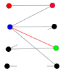
      Figure 9. Determining the neighbors of the Match.

   2. If $a_{t}(J^{+})=0$, then no node is added to the matching, and we just set

      $$G^{\prime}_{t+1}=G^{\prime}_{t},\quad E_{t+1}=E_{t},\quad A_{t+1}^{+}=A^{+}_{t}\quad\mbox{ and }\quad A_{t+1}^{-}=A^{-}_{t}.$$

3. We set $t:=t+1$ and go back to step 1.

The procedure terminates at time $n$. At that time, we end up with a bipartite multi-graph $G:=G_{n}=(V,E_{n})$, since all half-edges have been completed. We then have the following result,

Proposition 1.

Suppose that the degree distributions $\mathbf{d}^{+}:=(d^{+}(1),...,d^{+}(n))$ and $\mathbf{d}^{-}(d^{-}(1),...,d^{-}(n))$ are graphical, namely, they can lead to a bipartite graph $G$ and set

$$\mathscr{G}(\mathbf{d}^{+},\mathbf{d}^{-}) =\left\{\mbox{bipartite graphs $\hat{G}$ on $V$ having degree distributions $\mathbf{d}^{+}$ and $\mathbf{d}^{-}$}\right\};$$

$$g(\mathbf{d}^{+},\mathbf{d}^{-}) =\mbox{Card }\mathscr{G}(\mathbf{d}^{+},\mathbf{d}^{-}).$$

Let $G$ be the resulting mutligraph of the construction of Section 4. Then, for any $\hat{G}\in\mathscr{G}(\mathbf{d}^{+},\mathbf{d}^{-})$ we get that

(4) $${\mathbb{P}}\left[G=\hat{G}\mid\mbox{$G$ is a graph}\right]={1\over g(\mathbf{d}^{+},\mathbf{d}^{-})},$$

in other words, conditionally on generating a graph, the construction produces graphs uniformly on the set of graphs having degree distributions $\mathbf{d}^{+}$ and $\mathbf{d}^{-}$.

Proof.

At each step, the procedure of uniform choice of the nodes $J^{+}$ and possibly $J^{-}$, in the steps 1a) and 2a) above, is exactly the uniform pairing procedure, as described in [22, 29]. From the so-called independence property in [29], the resulting multigraph $G$ is then a bipartite realization of the configuration model.

The uniform property (4) follows: specifically, Theorem 2.3 in [11] show how to properly build a directed graph from two given degree distributions while ensuring that these distributions are graphical. It is then shown in Proposition 4.1 in [11], that when the considereddistributions admit a variance (so that simple graph realizations of the CM do exist), the directed Configuration Model also preserves the uniform property on simple graphs. All that is left is to use the natural bijection between directed and bipartite graphs (as an example, see the bijection using matrices in [8]). $\blacksquare$

At time $n$, we necessarily get that $|M^{+}_{n}|=|M^{-}_{n}|$ and $U^{+}_{n}=\emptyset$. Also, as in the construction of Section 3, if $|I^{+}_{n}|\neq 0$, then there are at time $n$, as many undetermined nodes on the right-hand side as of isolated nodes on the left-hand side. We then set all undetermined nodes on the right-hand side as isolated, i.e., we set $I^{-}_{n}:=U^{-}_{n}$, and then $I_{n}=I^{+}_{n}\cup I^{-}_{n}$. We again obtain that $|M_{n}|+|I_{n}|=2n.$ Similarly to (2), the matching coverage ${\mathbf{M}}^{n}_{\Phi}(\xi^{+},\xi^{-})$ is then the proportion of initial nodes that ended up in the matching at the termination time $n$, that is,

(5) $${\mathbf{M}}^{n}_{\Phi}(\xi^{+},\xi^{-})={|M_{n}|\over 2n}=1-{|I_{n}|\over 2n}\cdot$$

5. Measure-valued representations

Fix a matching criterion $\Phi$. To compare the two constructions, we define two measure-valued processes. For all $0\leq t\leq n$, we define the following point measures:

• We let $\tilde{\mu}^{+}_{t}$ (resp., $\tilde{\mu}^{-}_{t}$) be the empirical degree distribution of all undetermined nodes at $t$ on the left-hand (resp., right-hand) side in the remaining graph $\tilde{G}_{t}$ defined in Section 3, that is,

  (6) $$\tilde{\mu}^{+}_{t}=\sum_{\tilde{v}^{+}\in\tilde{U}_{t}^{+}}\delta_{d_{t}(\tilde{v}^{+})},\quad\tilde{\mu}^{-}_{t}=\sum_{{\tilde{v}^{-}\in\tilde{U}_{t}^{-}}}\delta_{d_{t}(\tilde{v}^{-})}.$$

• We let $\tilde{\mu}^{+}_{t}$ (resp., $\tilde{\mu}^{-}_{t}$) be the empirical distribution representing the availabilities of all undetermined nodes at $t$ on the left-hand (resp., right-hand) side, as defined in Section 4:

  (7) $$\mu^{+}_{t}=\sum_{v^{+}\in U_{t}^{+}}\delta_{a_{t}(v^{+})},\quad\mu^{-}_{t}=\sum_{{v^{-}\in U_{t}^{-}}}\delta_{a_{t}(v^{-})}.$$

Now, observe that in the construction of Section 3, the isolated nodes at $t=n$ on the right-hand side are precisely the undetermined nodes having degree zero at the end of the construction. All the same, in the construction of Section 4 the isolated nodes at $t=n$ are the undetermined nodes having degree zero at the final step. Second, by construction there are in both cases, as many isolated nodes on both sides of the bipartition. Therefore, we get that

$$|\tilde{I}_{n}|=2\tilde{\mu}^{-}_{n}(\{0\})\quad\mbox{ and }\quad|I_{n}|=2\mu^{-}_{n}(\{0\}).$$

All in all, it follows from (2) and (5), that the two matching coverages are respectively given by

(8) $$\tilde{\mathbf{M}}^{n}_{\Phi}(G) =1-{\tilde{\mu}^{-}_{n}(\{0\})\over n};$$

(9) $${\mathbf{M}}^{n}_{\Phi}(\xi^{+},\xi^{-}) =1-{\mu^{-}_{n}(\{0\})\over n}\cdot$$

It is easily seen from the very algorithm of Section 3, that the process $\left(\tilde{G}_{t},\,t\in\llbracket 0,n\rrbracket\right)$ is Markov, but that the process $\left((\tilde{\mu}_{t}^{+},\tilde{\mu}^{-}_{t}),\,t\in\llbracket 0,n\rrbracket\right)$, alone, is not. Indeed, for any $t$ the evolution from the graph $\tilde{G}_{t}$ to the graph $\tilde{G}_{t+1}$ depends on the whole connectivity of $\tilde{G}_{t}$ (which node is connected to which one), not only on its degree distribution $\tilde{\mu}_{t}$.

On the other hand, regarding the construction of Section 4 we have the following,

Proposition 2.

The process $\left((\mu_{t}^{+},\mu^{-}_{t}),\,t\in\llbracket 0,n\rrbracket\right)$ is Markov.

Proof.

Fix $t\in\llbracket 0,n\rrbracket$. Between times $t$ and $t+1$, the measures $\mu^{+}_{t}$ and $\mu^{-}_{t}$ are updated as follows:

• If the drawn node $J^{+}$ on the left-hand side has a positive availability (Steps 1a) and then 2a) in the above procedure), then we first delete from $\mu^{+}_{t}$ the atom corresponding to the newly matched node $J^{+}$, and from $\mu^{-}_{t}$, the one corresponding to its match $J^{-}$ on the right-hand side. Then, $\mu^{+}_{t+1}$ is obtained by updating the availabilities of the unmatched nodes $J^{+}_{1},...,J^{+}_{\ell}$ connected to $J^{-}$. We obtain that

  (10) $$\left\{\begin{array}[]{ll}\mu_{t+1}^{+}&=\mu_{t}^{+}-\delta_{a_{t}(J^{+})}+\displaystyle\sum_{l=1}^{\ell}\left(\delta_{a_{t}\left(J^{+}_{l}\right)-E^{+}_{l}}-\delta_{a_{t}\left(J^{+}_{l}\right)}\right);\\ \mu_{t+1}^{-}&=\mu_{t}^{-}-\delta_{a_{t}(J^{-})}+\displaystyle\sum_{l=1,\,l\neq\sigma(m)}^{k}\left(\delta_{a_{t}\left(J^{-}_{l}\right)-E^{-}_{l}}-\delta_{a_{t}\left(J^{-}_{l}\right)}\right),\end{array}\right.$$

  where sums over empty sets are understood as null.

• Now, if $J^{+}$ has a zero availability (Steps 1b) and 2b) in the above procedure), then this node switches from the set $U_{t}$ to the set $I_{t+1}$, and so the corresponding atom is deleted from the measure $\mu^{+}_{t}$. Thus we get

  (11) $$\left\{\begin{array}[]{ll}\mu_{t+1}^{+}&=\mu_{t}^{+}-\delta_{a_{t}(J^{+})}\,;\\ \\ \mu_{t+1}^{-}&=\mu_{t}^{-}\,.\end{array}\right.$$

In the above recurrence equations, the choice of $J^{+}$ is a measurable function of $\mu^{+}_{t}$ and of draws that are independent of $\sigma\left((\mu^{+}_{s},\mu^{+}_{s}),\,s\leq t\right)$. Also, in (10), from the assumption that the matching criterion is local, the choice of $J^{-}$ is also a measurable function of the availabilities of the nodes of the right-hand side, i.e., of $\mu^{-}_{t}$, together with a draw that is independent of $\sigma\left((\mu^{+}_{s},\mu^{+}_{s}),\,s\leq t\right)$, see (1). All the same, from the very construction of the uniform pairing procedure, the values of $J^{+}_{1},...,J^{+}_{\ell}$, $E^{+}_{1},...E^{+}_{\ell}$, $J^{-}_{l},\,l\in\llbracket 1,k\rrbracket\setminus\{\sigma(m)\}$ and $E^{-}_{l},\,l\in\llbracket 1,k\rrbracket\setminus\{\sigma(m)\}$ are measurable functions of $\mu_{t}^{+},\mu_{t}^{-}$, and draws that are independent of $\sigma\left((\mu^{+}_{s},\mu^{+}_{s}),\,s\leq t\right)$. Therefore, (10-11) defines a proper Markov transition. $\blacksquare$

As we have just proven, the measure-valued representation is Markov in the second construction, not in the first one. However, as the following result demonstrates, there is a close connexion between the two processes,

Theorem 1.

Let $n$ be a positive integer, and $\tilde{G}$ be a balanced bipartite graph of size $2n$, and let $\mathbf{d}^{+}$ and $\mathbf{d}^{-}$ be the respective degree distributions of the left-hand and right-hand side. Let $\left((\tilde{\mu}^{+}_{t},\tilde{\mu}^{-}_{t}),\,t\in\llbracket 0,n\rrbracket\right)$ and $\left((\mu^{+}_{t},\,\mu^{-}_{t}),\,t\in\llbracket 0,n\rrbracket\right)$ be the two measure-valued stochastic processes, defined respectively by (6) and (7), having common initial values

$$\tilde{\mu}_{0}^{+}=\mu_{0}^{+}=\sum_{i=1}^{n}\delta_{d^{+}(i)}\quad\mbox{ and }\quad\tilde{\mu}_{0}^{-}=\mu_{0}^{-}=\sum_{i=1}^{n}\delta_{d^{-}(i)}.$$

Let $G$ be the resulting multigraph of the second construction. Then, for any $t\in\llbracket 0,n\rrbracket$ and any couple of measures $(\nu^{+},\nu^{-})$, we get that

$${\mathbb{P}}\left[(\mu^{+}_{t},\mu^{-}_{t})=(\nu^{+},\nu^{-})\mid G=\tilde{G}\right]={\mathbb{P}}\left[(\tilde{\mu}^{+}_{t},\tilde{\mu}^{-}_{t})=(\nu^{+},\nu^{-})\right].$$

Proof.

Suppose that $G=\tilde{G}$, that is, the second construction eventually produces the graph $\tilde{G}$. We index the nodes of $V$ consistently in the two constructions.The initial couples of measures $(\tilde{\mu}_{0}^{+},\tilde{\mu}_{0}^{-})$ and $(\mu_{0}^{+},\mu_{0}^{-})$ coincide by assumption, and we then proceed by induction on $t$.

Suppose that, at some time $t\in\llbracket 0,n-1\rrbracket$ we have

(12) $$\tilde{U}_{t}=U_{t}\quad\mbox{ and }\quad a_{t}(v)=d_{t}(v)\,\mbox{ for all }\,v\mbox{ in }\tilde{U}_{t}=U_{t}.$$

We will construct a coupling such that (12) holds also at time $t+1$. For this, first, as $\tilde{U}_{t}=U_{t}$, at steps $\tilde{1}$ and step $1$ respectively, we can set a common realization of a uniform draw on $\llbracket 1,|U^{+}_{t}|\rrbracket$, leading to the same values for $\tilde{J}^{+}$ and $J^{+}$. Then,

• If $a_{t}(J^{+})>0$, at step 1a), as $G=\tilde{G}$ the uniform pairing procedure leads to the same set of neighbors for $J^{+}$ as in $\tilde{G}$, namely $J^{-}_{1}=\tilde{J}^{-}_{1},...,J^{-}_{k}=\tilde{J}^{-}_{k}$. Then, as $d_{t}(\tilde{J}^{+})=a_{t}(J^{+})>0$, at steps $\tilde{2}$a) and 2a) respectively, we can set the same value for $\tilde{J}^{-}$ and $J^{-}$ in $\tilde{U}^{-}_{t}=\tilde{U}^{-}_{t}$, using the common rule $\Phi$ and the the same uniform draw for the permutation $\sigma$. Finally, as $G=\tilde{G}$ the uniform pairing procedure leads to the same set of neighbors for $J^{-}$ (aside from $J^{+}$) as in $\tilde{G}$, namely $J^{+}_{1}=\tilde{J}^{+}_{1},...,J^{+}_{k}=\tilde{J}^{+}_{\ell}$. We then obtain that

  $$\tilde{U}_{t+1}=\tilde{U}_{t}\setminus\{\tilde{J}^{+},\tilde{J}^{-}\}=U_{t}\setminus\{J^{+},J^{-}\}=U_{t+1}.$$

  Second, as $G$ is a graph we get that $k=d_{t}(\tilde{J}^{+})=a_{t}(J^{+})$ and $\ell=d_{t}(\tilde{J}^{-})=a_{t}(J^{-})$. Moreover, for any $l\in\llbracket 1,k\rrbracket\setminus\{\sigma(m)\}$, at step 1a) we obtain that

  $$a_{t+1}(J^{-}_{l})=a_{t}(J^{-}_{l})-E^{-}_{l}=a_{t}(J^{-}_{l})-1=d_{t}(J^{-}_{l})-1=a_{t+1}(J^{-}_{l}).$$

  All the same, for any $l\in\llbracket 1,\ell\rrbracket\setminus\{\sigma(m)\}$, at step 2a) we obtain that

  $$a_{t+1}(J^{+}_{l})=a_{t}(J^{+}_{l})-E^{+}_{l}=a_{t}(J^{+}_{l})-1=d_{t}(J^{+}_{l})-1=a_{t+1}(J^{+}_{l}).$$

  Last, for any $v\in U_{t+1}\setminus\{J^{+}_{1},...,J^{+}_{\ell},J^{-}_{1},...,J^{-}_{k}\}$ we get that

  $$a_{t+1}(v)=a_{t}(v)=d_{t}(v)=d_{t+1}(v).$$

• If $a_{t}(J^{+})=0$, then we obtain that

  $$\tilde{U}_{t+1}=\tilde{U}_{t}\setminus\{\tilde{J}^{+}\}=U_{t}\setminus\{J^{+}\}=U_{t+1}$$

  and for all $v\in\tilde{U}_{t+1}=U_{t+1}$,

  $$a_{t+1}(v)=a_{t}(v)=d_{t}(v)=d_{t+1}(v).$$

In all cases, (12) holds at step $t+1$.

To conclude, we can then construct a coupling such that (12) holds for all $t\in\llbracket 0,n\rrbracket$. From the very definitions (6) and (7), this implies in particular that $(\tilde{\mu}_{t}^{+},\tilde{\mu}_{t}^{-})=(\mu_{t}^{+},\mu_{t}^{-})$ for all $t\in\llbracket 0,n\rrbracket$. This concludes the proof. $\blacksquare$

We are now in a position to estimate the matching coverage of local algorithms on a given bipartite graph, as the size $2n$ of the latter grows to infinity, using an approximation of the Markov chain $\left((\mu_{t}^{+},\mu^{-}_{t}),\,t\in\llbracket 0,n\rrbracket\right)$. Our strategy is as follows: first, using a procedure that is closely related to the Differential Equation Method of [29], we can exploit the Markov property, Proposition 2, to derive a large-graph approximation of the (suitably scaled) Markov chain $\left((\mu_{t}^{+},\mu^{-}_{t}),\,t\in\llbracket 0,n\rrbracket\right)$ as the solution of an ODE, which we introduce in Section 6. Then, we use the relations (2) and (5), together with our coupling result, Theorem 1, to approximate the matching coverage for a given graph $G$ and a given matching criterion $\Phi$, by an explicit function of the measure-valued solution of the ODE under consideration - see (25) below. As examples, we then study the two particular cases of local algorithms, greedy and minres, introduced in Definition 1.

6. Hydrodynamic approximation

In this section, we introduce our hydrodynamic approximation of the construction of Section 4, namely, a system of measure-valued ODE that we will use as an approximation of the behavior of the process $\left((\mu_{t}^{+},\mu^{-}_{t}),\,t\in\llbracket 0,n\rrbracket\right)$.

Definition 2 (Hydrodynamic approximation).

Fix a local matching algorithm $\Phi$. Let for all $\varphi:{\mathbb{R}}\to{\mathbb{R}}$, $\mu^{+},\,\mu^{-}\in{\mathcal{M}}({\mathbb{N}})$, $k\in{\mathbb{N}}$ and $t\geq 0$,

$$F^{\Phi}_{\varphi,\mu^{-}}(k)={\mathbb{E}}\left[\varphi\left(a_{t}(J^{-})-1\right)\,|\,a_{t}(J^{+})=k,\,(\mu^{+}_{t},\mu^{-}_{t})=(\mu^{+},\mu^{-})\right]\mathbf{1}_{{\mathbb{N}}^{*}}(k).$$

A hydrodynamic approximation of the algorithm is a solution $\left((\bar{\mu}^{+},\bar{\mu}^{-}),\,t\in[0,1]\right)$ in $\mathrm{D}\left([0,1],({\mathcal{M}}({\mathbb{N}}))^{2}\right)$, of the following family of systems of ODE’s: for all $s\in[0,1]$,

(13) $$\left\{\begin{array}[]{ll}\displaystyle{\text{ d}\left\langle\bar{\mu}^{+}_{s},\varphi\right\rangle\over\text{ d}s}&=\displaystyle-{\left\langle\bar{\mu}^{+}_{s},\varphi\right\rangle\over\left\langle\bar{\mu}^{+}_{s},\mathbf{1}\right\rangle}-{\left\langle\bar{\mu}^{+}_{s},F^{\Phi}_{X,\bar{\mu}^{-}_{s}}\right\rangle\over\left\langle\bar{\mu}^{+}_{s},\mathbf{1}\right\rangle}{\left\langle\bar{\mu}^{+}_{s},X\Delta\varphi\right\rangle\over\left\langle\bar{\mu}^{+}_{s},X\right\rangle}\\ \displaystyle{\text{ d}\left\langle\bar{\mu}^{-}_{s},\varphi\right\rangle\over\text{ d}s}&=\displaystyle-{\left\langle\bar{\mu}^{+}_{s},F^{\Phi}_{\varphi,\bar{\mu}^{-}_{s}}\right\rangle\over\left\langle\bar{\mu}^{+}_{s},\mathbf{1}\right\rangle}-{\left\langle\bar{\mu}^{+}_{s},X\right\rangle\over\left\langle\bar{\mu}^{+}_{s},\mathbf{1}\right\rangle}{\left\langle\bar{\mu}^{-}_{s},X\Delta\varphi\right\rangle\over\left\langle\bar{\mu}^{-}_{s},X\right\rangle}\end{array}\right.,\,\varphi\in\mathcal{B}_{b}({\mathbb{N}})\cup\{X,X^{2}\}.$$

6.1. Heuristics: a large-graph limit

Properly showing the convergence of the sequence of CTMC’s $\left((\mu_{t}^{+},\mu^{-}_{t}),\,t\in\llbracket 0,n\rrbracket\right)$, properly scaled, to a solution of (13), lies beyond the scope of this paper - and so does the proof of existence and uniqueness of the latter. However, let us provide heuristic arguments to intuitively justify the form of the right-hand side of (13) as an approximation of the dynamics of our construction. To do so, we study for all $\varphi:{\mathbb{R}}\to{\mathbb{R}}$, the drift of the process $\left(\left\langle\mu_{t}^{+},\varphi\right\rangle,\,t\in\llbracket 0,n\rrbracket\right)$, the drift of $\left(\left\langle\mu_{t}^{+},\varphi\right\rangle,\,t\in\llbracket 0,n\rrbracket\right)$ can be addressed similarly. Fix $\varphi:{\mathbb{R}}\to{\mathbb{R}}$, two measures $\mu^{+}$ and $\mu^{-}$ and $t\in\llbracket 0,n-1\rrbracket$. We address the terms on the right-hand side of (10) separately:

• First, as $J^{+}$ is drawned uniformly across among all nodes on the ‘+’ side, we easily get that

  $${\mathbb{E}}\left[\varphi\left(a_{t}(J^{+})\right)\,|\,(\mu^{+}_{t},\mu^{-}_{t})=(\mu^{+},\mu^{-})\right] =\sum_{k=0}^{n}\varphi(k){\mathbb{P}}\left[a_{t}(J^{+})=k\,|\,(\mu^{+}_{t},\mu^{-}_{t})=(\mu^{+},\mu^{-})\right]$$

  (14) $$=\sum_{k=0}^{n}\varphi(k)\frac{\mu^{+}(k)}{\left\langle\mu^{+},\mathbf{1}\right\rangle}=\frac{\left\langle\mu^{+},\varphi\right\rangle}{\left\langle\mu^{+},\mathbf{1}\right\rangle}\cdot$$

• Now, first observe that as the number of nodes grows large the probability of having multi-edges in the CM vanishes (see e.g. [22]). In particular, with overwhelming probability, $J^{-}$ has $a_{t}(J^{-})-1$ different neighbors which are not $J^{+}$, so we can make the approximation

  (15) $${\mathbb{E}}\left[\sum_{l=1}^{\ell}\left(\varphi\left(a_{t}\left(J^{+}_{l}\right)-E^{+}_{l}\right)-\varphi\left(a_{t}\left(J^{+}_{l}\right)\right)\right)\,|\,(\mu^{+}_{t},\mu^{-}_{t})=(\mu^{+},\mu^{-})\right]\\ \simeq{\mathbb{E}}\left[\sum_{l=1}^{a_{t}\left(J^{-}\right)-1}\left(\varphi\left(a_{t}\left(J^{+}_{l}\right)-1\right)-\varphi\left(a_{t}\left(J^{+}_{l}\right)\right)\right)\,|\,(\mu^{+}_{t},\mu^{-}_{t})=(\mu^{+},\mu^{-})\right].$$

  Second, for a large $n$, independent sampling of half-edges with replacement are asymptotically equivalent to the sampling without replacement that are inherent to the procedure of uniform pairing of half-edges. Therefore, it follows from Wald’s identity that

  (16) $${\mathbb{E}}\left[\sum_{l=1}^{a_{t}\left(J^{-}\right)-1}\left(\varphi\left(a_{t}\left(J^{+}_{l}\right)-1\right)-\varphi\left(a_{t}\left(J^{+}_{l}\right)\right)\right)\,|\,(\mu^{+}_{t},\mu^{-}_{t})=(\mu^{+},\mu^{-})\right]\\ =-{\mathbb{E}}\left[\sum_{l=1}^{a_{t}\left(J^{-}\right)-1}\Delta\varphi\left(a_{t}\left(J^{+}_{l}\right)\right)\,|\,(\mu^{+}_{t},\mu^{-}_{t})=(\mu^{+},\mu^{-})\right]\\ \simeq-{\mathbb{E}}\left[\Delta\varphi\left(a_{t}\left(J^{+}_{1}\right)\right)\,|\,(\mu^{+}_{t},\mu^{-}_{t})=(\mu^{+},\mu^{-})\right]{\mathbb{E}}\left[a_{t}\left(J^{-}\right)-1\,|\,(\mu^{+}_{t},\mu^{-}_{t})=(\mu^{+},\mu^{-})\right].$$

  But as the choice of half-edges are uniform, $a_{t}(J_{1}^{+})$ follows the size-biased distribution relative to $\mu^{+}$, so we can write that

  $${\mathbb{E}}\left[\Delta\varphi\left(a_{t}\left(J^{+}_{1}\right)\right)\,|\,\mu^{+}_{t}=\mu^{+},\,\mu^{-}_{t}=\mu^{-}\right] =\sum_{a=1}^{n}\Delta\varphi(a){\mathbb{P}}\left[a_{t}\left(J^{+}_{1}\right)=a\,|\,\mu^{+}_{t}=\mu^{+},\,\mu^{-}_{t}=\mu^{-}\right]$$

  (17) $$=\sum_{a=1}^{n}\Delta\varphi(a)\frac{k\mu^{+}(k)}{\left\langle\mu^{+},X\right\rangle}={\left\langle\mu^{+},X\Delta\varphi\right\rangle\over\left\langle\mu^{+},X\right\rangle}\cdot$$

  Also, in view of the above remark we obtain that

  $${\mathbb{E}}\left[a_{t}\left(J^{-}\right)-1\,|\,(\mu^{+}_{t},\mu^{-}_{t})=(\mu^{+},\mu^{-})\right]\\ \begin{aligned} &=\sum_{k=0}^{n}{\mathbb{E}}\left[a_{t}\left(J^{-}\right)-1\,|\,a_{t}(J^{+})=k,\,(\mu^{+}_{t},\mu^{-}_{t})=(\mu^{+},\mu^{-})\right]{\mathbb{P}}\left[a_{t}(J^{+})=k\,|\,(\mu^{+}_{t},\mu^{-}_{t})=(\mu^{+},\mu^{-})\right]\\ &=\sum_{k=0}^{n}F^{\Phi}_{X,\mu^{-}}(k){\mathbb{P}}\left[a_{t}(J^{+})=k\,|\,(\mu^{+}_{t},\mu^{-}_{t})=(\mu^{+},\mu^{-})\right]\\ &=\sum_{k=0}^{n}F^{\Phi}_{X,\mu^{-}}(k){\mu^{+}(k)\over\left\langle\mu^{+},\mathbf{1}\right\rangle}=\frac{\left\langle\mu^{+},F^{\Phi}_{X,\mu^{-}}\right\rangle}{\left\langle\mu^{+},\mathbf{1}\right\rangle}\cdot\end{aligned}$$

  Gathering this together with (16-17) into (15), we obtain that

  $${\mathbb{E}}\left[\sum_{l=1}^{\ell}\left(\varphi\left(a_{t}\left(J^{+}_{l}\right)-E^{+}_{l}\right)-\varphi\left(a_{t}\left(J^{+}_{l}\right)\right)\right)\,|\,(\mu^{+}_{t},\mu^{-}_{t})=(\mu^{+},\mu^{-})\right]\simeq-\frac{\left\langle\mu^{+},F^{\Phi}_{X,\mu^{-}}\right\rangle}{\left\langle\mu^{+},\mathbf{1}\right\rangle}{\left\langle\mu^{+},X\Delta\varphi\right\rangle\over\left\langle\mu^{+},X\right\rangle}\cdot$$

This, together with (14) in (10), yields to the following drift approximation:

(18) $${\mathbb{E}}\left[\left\langle\mu_{t+1}^{+},\varphi\right\rangle-\left\langle\mu_{t}^{+},\varphi\right\rangle\,|\,(\mu^{+}_{t},\mu^{-}_{t})=(\mu^{+},\mu^{-})\right]\simeq-\frac{\left\langle\mu^{+},\varphi\right\rangle}{\left\langle\mu^{+},\mathbf{1}\right\rangle}-\frac{\left\langle\mu^{+},F^{\Phi}_{X,\mu^{-}}\right\rangle}{\left\langle\mu^{+},\mathbf{1}\right\rangle}{\left\langle\mu^{+},X\Delta\varphi\right\rangle\over\left\langle\mu^{+},X\right\rangle}\cdot$$

Scaling.

Let us first emphasize the dependence in $n$ of the various parameters for a given graph of size $2n$, by adding a superscript $n$ to all variables involved. In particular, we denote respectively by $\mu_{t}^{n,+}$ and $\mu_{t}^{n,-}$, the two measures at time $t$. Let us denote for any $(\mu^{+},\mu^{-})$ and any $G:{\mathcal{M}}({\mathbb{N}})^{2}\to{\mathbb{R}}$ such that the following expectations exist, the drift

$${\mathscr{Q}}^{n}G\left(\mu^{+},\mu^{-}\right):={\mathbb{E}}\left[G\left(\mu_{t+1}^{n,+},\mu_{t+1}^{n,+}\right)-G\left(\mu_{t}^{n,+},\mu_{t}^{n,+}\right)\,|\,(\mu^{n,+}_{t},\mu^{n,-}_{t})=(\mu^{+},\mu^{-})\right],\quad t\geq 0.$$

Then, defining for any $\varphi\in\mathcal{B}_{b}({\mathbb{N}})\cup\{X,X^{2}\}$, the mapping

$$\Pi^{1}_{\varphi}:\begin{cases}{\mathcal{M}}({\mathbb{N}})^{2}&\longrightarrow{\mathbb{R}}\\ (\mu^{+},\mu^{-})&\longmapsto\left\langle\mu^{+},\varphi\right\rangle\end{cases}\,,$$

(18) can be rewritten as

(19) $$\mathscr{Q}^{n}\Pi^{1}_{\varphi}\left(\mu^{+},\mu^{-}\right)\simeq\mathscr{Q}\Pi^{1}_{\varphi}\left(\mu^{+},\mu^{-}\right):=-\frac{\left\langle\mu^{+},\varphi\right\rangle}{\left\langle\mu^{+},\mathbf{1}\right\rangle}-\frac{\left\langle\mu^{+},F^{\Phi}_{X,\mu^{-}}\right\rangle}{\left\langle\mu^{+},\mathbf{1}\right\rangle}{\left\langle\mu^{+},X\Delta\varphi\right\rangle\over\left\langle\mu^{+},X\right\rangle}\cdot$$

Let us define the corresponding scaled, and interpolated, continuous-time processes: for all $t\in[0,1]$, we let

(20) $$\bar{\mu}^{n,+}_{t}={1\over n}\mu^{n,+}_{\left\lfloor nt\right\rfloor}\quad\mbox{ and }\quad\bar{\mu}^{n,-}_{t}={1\over n}\mu^{n,-}_{\left\lfloor nt\right\rfloor}.$$

This scaling corresponds to an acceleration in time of factor $n$ (each consecutive steps being $1/n$ units of time apart), compensated by a scaling in space, of the same magnitude, the weight of each atom being divided by $n$. As the approximate drift in the right-hand side of (19) is independent of $n$ and bilinear in $(\mu^{+},\mu^{-})$, using martingale representations, after scaling and taking $n$ to infinity, it is then standard (again, see the Differential equation method in [29]), that any limiting process $\left(\bar{\mu}_{t},\,t\in[0,1]\right):=\left((\bar{\mu}^{+}_{t},\bar{\mu}^{-}_{t}),\,t\in[0,1]\right)$ of $\left(\bar{\mu}^{n}_{t},\,t\in[0,1]\right):=\left((\bar{\mu}^{n,+}_{t},\bar{\mu}^{n,-}_{t}),\,t\in[0,1]\right)$ solves the integral equation

$$\left\langle\bar{\mu}^{+}_{t},\varphi\right\rangle-\left\langle\bar{\mu}^{+}_{0},\varphi\right\rangle=\Pi^{1}_{\varphi}(\bar{\mu}_{t})-\Pi^{1}_{\varphi}(\bar{\mu}_{0})=\int_{0}^{t}\mathscr{Q}\Pi^{1}_{\varphi}\left(\bar{\mu}_{s}\right)\text{ d}s,\quad t\in[0,1],$$

if a solution does exist. Plugging (19) in the above, and differentiating in $t$, yields to the first equation of (13) at all $t$ and for all $\varphi$. Retrieving the second equation of (13) can be done in a similar fashion.

6.2. Hydrodynamic approximation for particular local algorithms

We now make precise the form of the systems of ODEs (13) for the two particular local algorithms introduced in Definition 1. We address successively $\Phi=\textsc{Greedy}$ and $\Phi=\textsc{Minres}$.

6.2.1. $\Phi=\textsc{Greedy}$.

For any $(\mu^{+},\mu^{-})\in{\mathcal{M}}({\mathbb{N}})^{2}$, $t\in[0,1]$ and any $k\in{\mathbb{N}}^{*}$, given that $\mu^{+}_{t}=\mu^{+}$, $\mu^{-}_{t}=\mu^{-}$ and that the degree of $J^{+}$ is $k>0$, by the very definition of the uniform pairing procedure, the match $J^{-}$ of $J^{+}$ is just determined by a uniform draw of one of its half-edge. Thus its availability $a_{t}(J^{-})$ at $t$ follows the size-biased distribution associated to $\mu^{-}$, namely we get that for all $a\in{\mathbb{N}}$,

$${\mathbb{P}}\left[a_{t}(J^{-})=a\,|\,a_{t}(J^{+})=k,\,(\mu^{+}_{t},\mu^{-}_{t})=(\mu^{+},\mu^{-})\right]={a\mu^{-}(a)\over\left\langle\mu^{-},X\right\rangle}\cdot$$

Consequently, we get that for all $k\in{\mathbb{N}}$ and $\varphi\in\mathcal{B}_{b}({\mathbb{N}})\cup\{X,X^{2}\}$,

$$F^{\scriptsize{\textsc{greedy}}}_{\varphi,\mu^{-}}(k) ={\mathbb{E}}\left[\varphi\left(a_{t}(J^{-})-1\right)\,|\,K^{+}=k,\,\mu^{-}_{t}=\mu^{-}\right]$$

$$=\sum_{a\in{\mathbb{N}}}\varphi(a-1){a\mu^{-}(a)\over\left\langle\mu^{-},X\right\rangle}\mathbf{1}_{{\mathbb{N}}^{*}}(k)={\left\langle\mu^{-},X\tau_{1}\varphi\right\rangle\over\left\langle\mu^{-},X\right\rangle}\mathbf{1}_{{\mathbb{N}}^{*}}(k),$$

where we denote $\tau_{1}\varphi(x)=\varphi(x-1)$ for all $x$. Plugging this into (13) we obtain that for all $t\leq 1$,

(21) $$\begin{cases}\displaystyle{\text{ d}\left\langle\bar{\mu}^{+}_{s},\varphi\right\rangle\over\text{ d}s}&=\displaystyle-{\left\langle\bar{\mu}^{+}_{s},\varphi\right\rangle\over\left\langle\bar{\mu}^{+}_{s},\mathbf{1}\right\rangle}-{\left\langle\bar{\mu}^{+}_{s},\mathbf{1}_{{\mathbb{N}}^{*}}\right\rangle\over\left\langle\bar{\mu}^{+}_{s},\mathbf{1}\right\rangle}{\left\langle\bar{\mu}^{-}_{s},X^{2}-X\right\rangle\over\left\langle\bar{\mu}^{-}_{s},X\right\rangle}{\left\langle\bar{\mu}^{+}_{s},X\Delta\varphi\right\rangle\over\left\langle\bar{\mu}^{+}_{s},X\right\rangle};\\ \\ \displaystyle{\text{ d}\left\langle\bar{\mu}^{-}_{s},\varphi\right\rangle\over\text{ d}s}&=\displaystyle-{\left\langle\bar{\mu}^{-}_{s},X\tau_{1}\varphi\right\rangle\over\left\langle\bar{\mu}^{-}_{s},X\right\rangle}{\left\langle\bar{\mu}^{+}_{s},\mathbf{1}_{{\mathbb{N}}^{*}}\right\rangle\over\left\langle\bar{\mu}^{+}_{s},\mathbf{1}\right\rangle}-{\left\langle\bar{\mu}^{+}_{s},X\right\rangle\over\left\langle\bar{\mu}^{+}_{s},\mathbf{1}\right\rangle}{\left\langle\bar{\mu}^{-}_{s},X\Delta\varphi\right\rangle\over\left\langle\bar{\mu}^{-}_{s},X\right\rangle}\\ \\ &=\displaystyle-{\left\langle\bar{\mu}^{-}_{s},X\varphi\right\rangle\over\left\langle\bar{\mu}^{-}_{s},X\right\rangle}{\left\langle\bar{\mu}^{+}_{s},\mathbf{1}_{{\mathbb{N}}^{*}}\right\rangle\over\left\langle\bar{\mu}^{+}_{s},\mathbf{1}\right\rangle}-{\left\langle\bar{\mu}^{+}_{s},X-\mathbf{1}_{{\mathbb{N}}^{*}}\right\rangle\over\left\langle\bar{\mu}^{+}_{s},\mathbf{1}\right\rangle}{\left\langle\bar{\mu}^{-}_{s},X\Delta\varphi\right\rangle\over\left\langle\bar{\mu}^{-}_{s},X\right\rangle}\cdot\end{cases}$$

6.2.2. $\Phi=\textsc{Minres}$.

By the very definition of Minres, for all $(\mu^{+},\mu^{-})\in{\mathcal{M}}({\mathbb{N}})^{2}$, $t\in[0,1]$ and all $k\in{\mathbb{N}}^{*}$, conditional on $a_{t}(J^{+})=k$ and $(\mu^{+}_{t},\mu^{-}_{t})=(\mu^{+},\mu^{-})$, for all all $a\in{\mathbb{N}}^{*}$ $a_{t}(J^{-})\geq a$ means that in the uniform pairing procedure, none of the neighbors of $J^{+}$ are of availability strictly less than $a$. Thus, as in the large-graph limit, draws without replacement can be approximated by draws with replacement, and at each step, all the neighbors of $J^{+}$ have with overwhelming probability, a single neighbor on the right-hand side, we get tho the approximation

$${\mathbb{P}}\left[a_{t}(J^{-})\geq a\,|\,a_{t}(J^{+})=k,\,(\mu^{+}_{t},\mu^{-}_{t})=(\mu^{+},\mu^{-})\right]\simeq\left(\frac{\left\langle\mu^{-},X\mathbf{1}_{[a,+\infty)}\right\rangle}{\left\langle\mu^{-},X\right\rangle}\right)^{k}.$$

Therefore, we obtain that

$$F^{\scriptsize{\textsc{minres}}}_{\varphi,\mu}(k)= {\mathbb{E}}\left[\varphi\left(a_{t}(J^{-})-1\right)\,|\,a_{t}(J^{+})=k,\,(\mu^{+}_{t},\mu^{-}_{t})=(\mu^{+},\mu^{-})\right]$$

$$= \sum_{a\in{\mathbb{N}}^{*}}\varphi(a-1)\Biggl{(}{\mathbb{P}}\left[a_{t}(J^{-})\geq a\,|\,a_{t}(J^{+})=k,\,(\mu^{+}_{t},\mu^{-}_{t})=(\mu^{+},\mu^{-})\right]$$

$$\phantom{\sum_{a\in{\mathbb{N}}}\varphi(a-1)\Biggl{(}}\quad-{\mathbb{P}}\left[a_{t}(J^{-})\geq a+1\,|\,a_{t}(J^{+})=k,\,(\mu^{+}_{t},\mu^{-}_{t})=(\mu^{+},\mu^{-})\right]\biggl{)}$$

$$\simeq \sum_{a\in{\mathbb{N}}^{*}}\varphi(a-1)\left(\frac{\left\langle\mu^{-},X\mathbf{1}_{[a,+\infty)}\right\rangle^{k}-\left\langle\mu^{-},X\mathbf{1}_{[a+1,+\infty)}\right\rangle^{k}}{\left\langle\mu^{-},X\right\rangle^{k}}\right).$$

Plugging this into (13) yields to

(22) $$\begin{cases}\displaystyle{\text{ d}\left\langle\bar{\mu}^{+}_{s},\varphi\right\rangle\over\text{ d}s}\simeq&\displaystyle-{\left\langle\bar{\mu}^{+}_{s},\varphi\right\rangle\over\left\langle\bar{\mu}^{+}_{s},\mathbf{1}\right\rangle}\\ \\ &\displaystyle-{\left\langle\bar{\mu}^{+}_{s},X\Delta\varphi\right\rangle\over\left\langle\bar{\mu}^{+}_{s},X\right\rangle}\sum_{k\in{\mathbb{N}}}\sum_{a\in{\mathbb{N}}^{*}}\left(\frac{\left\langle\bar{\mu}^{-}_{s},X\mathbf{1}_{[a,+\infty)}\right\rangle^{k}-\left\langle\bar{\mu}^{-}_{s},X\mathbf{1}_{[a+1,+\infty)}\right\rangle^{k}}{\left\langle\bar{\mu}^{-}_{s},X\right\rangle^{k}}\right){(a-1)\bar{\mu}^{+}_{s}(k)\over\left\langle\bar{\mu}^{+}_{s},\mathbf{1}\right\rangle};\\ \\ \displaystyle{\text{ d}\left\langle\bar{\mu}^{-}_{s},\varphi\right\rangle\over\text{ d}s}\simeq&\displaystyle-\sum_{k\in{\mathbb{N}}}\sum_{a\in{\mathbb{N}}^{*}}\left(\frac{\left\langle\bar{\mu}^{-}_{s},X\mathbf{1}_{[a,+\infty)}\right\rangle^{k}-\left\langle\bar{\mu}^{-}_{s},X\mathbf{1}_{[a+1,+\infty)}\right\rangle^{k}}{\left\langle\bar{\mu}^{-}_{s},X\right\rangle^{k}}\right){(a-1)\bar{\mu}^{+}_{s}(k)\over\left\langle\bar{\mu}^{+}_{t},\mathbf{1}\right\rangle}\\ \\ &\displaystyle-{\left\langle\bar{\mu}^{+}_{s},X\right\rangle\over\left\langle\bar{\mu}^{+}_{s},\mathbf{1}\right\rangle}{\left\langle\bar{\mu}^{-}_{s},X\Delta\varphi\right\rangle\over\left\langle\bar{\mu}^{-}_{s},X\right\rangle}\cdot\end{cases}$$

6.3. Approximating the matching coverage

We are now ready to introduce our estimate of the matching coverage in the large-graph limit. Recall, that in the construction of Section 3, the isolated nodes at $t=n$ on the ‘-’ side are precisely the undetermined nodes having degree zero at the end of the construction. All the same, in the construction of Section 4 the isolated nodes at $t=n$ on the ‘-’ side are the undetermined nodes of the ‘-’ side having degree zero at the final step, because at completion of the algorithm, all half-edges have been paired.

Second, by construction there are in both cases, as many isolated nodes on both sides of the bipartition. Therefore, we get that

$$|\tilde{I}_{n}|=2\tilde{\mu}^{-}_{n}(\{0\})\quad\mbox{ and }\quad|I_{n}|=2\mu^{-}_{n}(\{0\}).$$

All in all, it follows from (2) and (5), that the two matching coverages are respectively given by

(23) $$\tilde{\mathbf{M}}^{n}_{\Phi}(G) =1-{\tilde{\mu}^{-}_{n}(\{0\})\over n};$$

(24) $${\mathbf{M}}^{n}_{\Phi}(\xi^{+},\xi^{-}) =1-{\mu^{-}_{n}(\{0\})\over n}=1-\bar{\mu}^{n,-}_{1}(\{0\})\cdot$$

Finally, in view of the large-graph approximation of Subsection 6.1 we can approximate the matching coverage of the second construction by

(25) $$\overline{\mathbf{M}}_{\Phi}(\xi^{+},\xi^{-}):=1-\bar{\mu}^{-}_{1}(\{0\}),$$

where $\left(\bar{\mu}_{t},\,t\in[0,1]\right)=\left((\bar{\mu}^{+}_{t},\bar{\mu}^{-}_{t}),\,t\in[0,1]\right)$ is a solution to (13). In turn, from our coupling result, Theorem 1, for a fixed graph $G$ the matching coverage after performing the first construction on $G$, given by (23), can be approximated by (25) for the same initial degree distribution.

7. Simulations

In this section, we illustrate and complete the above results by way of simulations. In Subsection 7.1, we test the empirical convergence of the matching coverage of the construction of Section 3, given by (23), under both algorithms Greedy and Minres, to the approximate matching size predicted by the ODEs through formula (25), for $G$ a $3$-regular graph. Then, in Subsection 7.2 we address, first, a comparison of the performances of the two algorithms, and second, the influence of the parameters on the matching size, along various degree distributions. Finally, in Subsection 7.3 we study the influence of the topology of the graph under consideration, by comparing the results when performing the algorithm of Section 3, and the algorithm of Section 4. We conclude with a comparison to the results in [23].

7.1. Convergence of the Matching Size : a case study on 3-regular graphs

In this section we use 3-regular graphs to the test the convergence of $\tilde{\mathbf{M}}^{n}_{\Phi}(G)$ to $\overline{\mathbf{M}}_{\Phi}(\delta_{3},\delta_{3})$, for $G$ a $3$-regular graph and the initial degree distribution $\mu_{0}^{+}=\mu_{0}^{-}=n\delta_{3}$, for $n$ the number of vertices on both sides. In this case we readily obtain that

(26) $$\bar{\mu}^{+}_{0}=\delta_{3}\quad\mbox{ and }\quad\bar{\mu}^{-}_{0}=\delta_{3}.$$

For Greedy, specializing the system (21) successively to $\varphi=\mathbf{1}_{\{0\}}$, $\varphi=\mathbf{1}_{\{1\}}$, $\varphi=\mathbf{1}_{\{2\}}$, $\varphi=\mathbf{1}_{3}$, yields to

(27) $$\begin{cases}\displaystyle\frac{\text{ d}\bar{\mu}^{+}_{s}(0)}{\text{ d}s}&=\displaystyle-\left(\frac{\bar{\mu}^{+}_{s}(0)}{m(\bar{\mu}^{+}_{s})}+\frac{m^{*}(\bar{\mu}^{+}_{s})}{m(\bar{\mu}^{+}_{s})}\left(\frac{Q(\bar{\mu}^{-}_{s})}{E(\bar{\mu}^{-}_{s})}-1\right)\frac{-\bar{\mu}^{+}_{s}(1)}{E(\bar{\mu}^{+}_{s})}\right);\\ \displaystyle\frac{\text{ d}\bar{\mu}^{+}_{s}(1)}{\text{ d}s}&=\displaystyle-\left(\frac{\bar{\mu}^{+}_{s}(1)}{m(\bar{\mu}^{+}_{s})}+\frac{m^{*}(\bar{\mu}^{+}_{s})}{m(\bar{\mu}^{+}_{s})}\left(\frac{Q(\bar{\mu}^{-}_{s})}{E(\bar{\mu}^{-}_{s})}-1\right)\frac{\bar{\mu}^{+}_{s}(1)-2\bar{\mu}^{+}_{s}(2)}{E(\bar{\mu}^{+}_{s})}\right);\\ \displaystyle\frac{\text{ d}\bar{\mu}^{+}_{s}(2)}{\text{ d}s}&=\displaystyle-\left(\frac{\bar{\mu}^{+}_{s}(2)}{m(\bar{\mu}^{+}_{s})}+\frac{m^{*}(\bar{\mu}^{+}_{s})}{m(\bar{\mu}^{+}_{s})}\left(\frac{Q(\bar{\mu}^{-}_{s})}{E(\bar{\mu}^{-}_{s})}-1\right)\frac{2\bar{\mu}^{+}_{s}(2)-3\bar{\mu}^{+}_{s}(3)}{E(\bar{\mu}^{+}_{s})}\right);\\ \displaystyle\frac{\text{ d}\bar{\mu}^{+}_{s}(3)}{\text{ d}s}&=\displaystyle-\left(\frac{\bar{\mu}^{+}_{s}(3)}{m(\bar{\mu}^{+}_{s})}+\frac{m^{*}(\bar{\mu}^{+}_{s})}{m(\bar{\mu}^{+}_{s})}\left(\frac{Q(\bar{\mu}^{-}_{s})}{E(\bar{\mu}^{-}_{s})}-1\right)\frac{3\bar{\mu}^{+}_{s}(3)}{E(\bar{\mu}^{+}_{s})}\right);\\[8.53581pt] \displaystyle\frac{\text{ d}\bar{\mu}^{-}_{s}(0)}{\text{ d}s}&=\displaystyle-\left(\frac{E(\bar{\mu}^{+}_{s})}{m(\bar{\mu}^{+}_{s})}-\frac{m^{*}(\bar{\mu}^{+}_{s})}{m(\bar{\mu}^{+}_{s})}\right)\frac{-\bar{\mu}^{-}_{s}(1)}{E(\bar{\mu}^{-}_{s})};\\ \displaystyle\frac{\text{ d}\bar{\mu}^{-}_{s}(1)}{\text{ d}s}&=\displaystyle-\left(\frac{\bar{\mu}^{-}_{s}(1)}{E(\bar{\mu}^{-}_{s})}\frac{m^{*}(\bar{\mu}^{+}_{s})}{m(\bar{\mu}^{+}_{s})}+\left(\frac{E(\bar{\mu}^{+}_{s})}{m(\bar{\mu}^{+}_{s})}-\frac{m^{*}(\bar{\mu}^{+}_{s})}{m(\bar{\mu}^{+}_{s})}\right)\frac{\bar{\mu}^{-}_{s}(1)-2\bar{\mu}^{-}_{s}(2)}{E(\bar{\mu}^{-}_{s})}\right);\\ \displaystyle\frac{\text{ d}\bar{\mu}^{-}_{s}(2)}{\text{ d}s}&=\displaystyle-\left(\frac{2\bar{\mu}^{-}_{s}(2)}{E(\bar{\mu}^{-}_{s})}\frac{m^{*}(\bar{\mu}^{+}_{s})}{m(\bar{\mu}^{+}_{s})}+\left(\frac{E(\bar{\mu}^{+}_{s})}{m(\bar{\mu}^{+}_{s})}-\frac{m^{*}(\bar{\mu}^{+}_{s})}{m(\bar{\mu}^{+}_{s})}\right)\frac{2\bar{\mu}^{-}_{s}(2)-3\bar{\mu}^{-}_{s}(3)}{E(\bar{\mu}^{-}_{s})}\right);\\ \displaystyle\frac{\text{ d}\bar{\mu}^{-}_{s}(3)}{\text{ d}s}&=-\displaystyle\left(\frac{3\bar{\mu}^{-}_{s}(3)}{E(\bar{\mu}^{-}_{s})}\frac{m^{*}(\bar{\mu}^{+}_{s})}{m(\bar{\mu}^{+}_{s})}+\left(\frac{E(\bar{\mu}^{+}_{s})}{m(\bar{\mu}^{+}_{s})}-\frac{m^{*}(\bar{\mu}^{+}_{s})}{m(\bar{\mu}^{+}_{s})}\right)\frac{3\bar{\mu}^{-}_{s}(3)}{E(\bar{\mu}^{-}_{s})}\right),\quad s\in[0,1],\end{cases}$$

where we denote for all $\mu\in{\mathcal{M}}({\mathbb{N}})$,

$$\begin{cases}m(\mu)&=\left\langle\mu,\mathbf{1}\right\rangle=\mu(0)+\mu(1)+\mu(2)+\mu(3);\\ m^{*}(\mu)&=\mu(1)+\mu(2)+\mu(3);\\ E(\mu)&=\left\langle\mu,X\right\rangle=\mu(1)+2\mu(2)+3\mu(3);\\ Q(\mu)&=\left\langle\mu,X^{2}\right\rangle=\mu(1)+4\mu(2)+9\mu(3).\end{cases}$$

(a) $\bar{\mu}^{+}_{s}(k)$ for $k=0,\dots,3$ and $s\in[0,1]$.

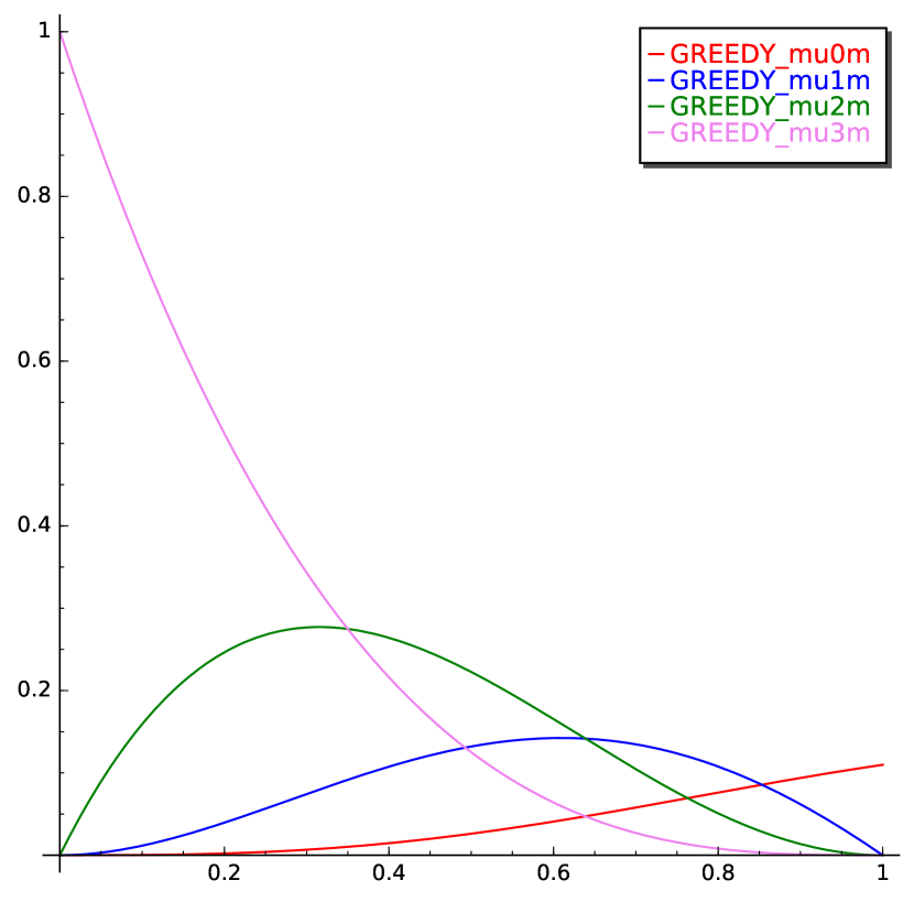
(b) $\bar{\mu}^{-}_{s}(k)$ for $k=0,\dots,3$ and $s\in[0,1]$.

Figure 10. Greedy-EDO results for $\bar{\mu}^{+}_{0}=\bar{\mu}^{-}_{0}=\delta_{3}$

A numerical resolution of the system of ODEs (27) is presented in Figure 10. We obtain the final value $\bar{\mu}^{-}_{1}(0)=0.1098$ (which is the final value of the red curve in the right-hand curve of Figure 10). From this, we deduce the approximate matching coverage

(28) $$\overline{\mathbf{M}}_{\textsc{Greedy}}(\delta_{3},\delta_{3})=1-\bar{\mu}^{-}_{1}(0)=0.8902.$$

Regarding Minres, similarly to (27) we can obtain a system of ODEs that specializes (22) to the case of the $3$-regular degree distribution, which we skip for brevity. From this, we deduce the approximate matching coverage

(29) $$\overline{\mathbf{M}}_{\textsc{Minres}}(\delta_{3},\delta_{3})=1-\bar{\mu}^{-}_{1}(0)=0.9378.$$

To illustrate the convergence of $\tilde{\mathbf{M}}^{n}_{\Phi}(G)$ to $\overline{\mathbf{M}}_{\Phi}(\delta_{3},\delta_{3})$ in both cases, we proceed as follows: for each value of $n$ from 10 to 10 000, we implement the bipartite configuration model to draw a $3$-regular graph as a realization of the CM. Then, we run each algorithm once and then plot the matching coverage. The following figures compile the evolution of the simulated matching coverages as the graph size $n$ grows large.

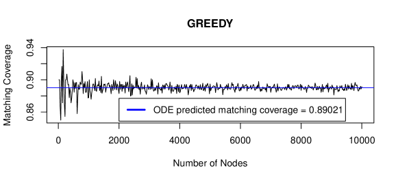
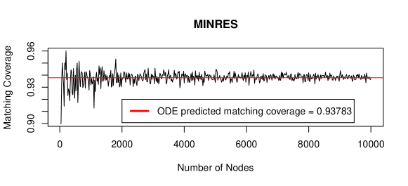
Figure 11. Matching coverage of Greedy as the graph size tends to $\infty$

Figure 12. Matching coverage of Minres as the graph size tends to $\infty$

As the graph gets larger, the fluctuations get smaller and smaller, heuristically showing the convergence of the matching coverage $\tilde{\mathbf{M}}^{n}_{\Phi}(G)$ to $\overline{\mathbf{M}}_{\Phi}(\delta_{3},\delta_{3})$, for both algorithms. To complete these results, for various graph sizes we ran $N=50$ iterations of the previous procedure. Means and standard deviations of the corresponding statistical distributions for $\tilde{\mathbf{M}}^{n}_{\Phi}(G)$, are given in Table 1

	Graph Size $n$	200	500	1000	3000	5000	$\overline{\mathbf{M}}_{\Phi}(\delta_{3},\delta_{3})$
$\tilde{\mathbf{M}}^{n}_{\textsc{Greedy}}(G)$	Mean	0.8904	0.8916	0.8911	0.8897	0.8898	0.8902
	Std Dev	0.0198	0.0109	0.009	0.0041	0.00311
$\tilde{\mathbf{M}}^{n}_{\textsc{Minres}}(G)$	Mean	0.9356	0.9365	0.9396	0.9378	0.9385	0.9378
	Std Dev	0.0148	0.0096	0.0052	0.0040	0.0025

Table 1. Recap. of Average Matching Size

Table 1 confirms the results that Figure 12 preluded. The shrinking of the standards deviation confirms the heuristic convergence to a deterministic value. It also stresses on the better performances of Minres with respect to Greedy for this particular degree distribution. In the next part, we develop this comparison for a larger range of degree distributions.

7.2. An Array of Degree Distributions

After the illustration of the convergence to the solution of the system of ODEs in the previous section, in this section we study the evolution of the performances of the two algorithms Greedy and Minres, along various degree distributions and various parameters.

Our procedure is the following: for each degree distribution, we implement the bipartite CM to generate a large graph (of size $n=10^{4}$ nodes), in which the degrees of the nodes form a $n$-sample of the prescribed degree distribution, after testing the graphicality of the latter degree distribution (i.e., the feasibility of the generation of the graph). For each distribution, we then ran $50$ iterations of both algorithms, following the first construction of Section 3.

Poisson distributions.

We first address the class of Poisson distributions, which are well know to be the asymptotic degree distributions of Erdös-Rényi graphs. Distributions of the matching coverage for the Greedy (respectively, Minres) algorithm are given in Figure 13(a) (resp., Figure 13(b)), for Poisson distributions of various parameters. For comparing the two algorithms, these distributions are gathered in Figure 13(c).

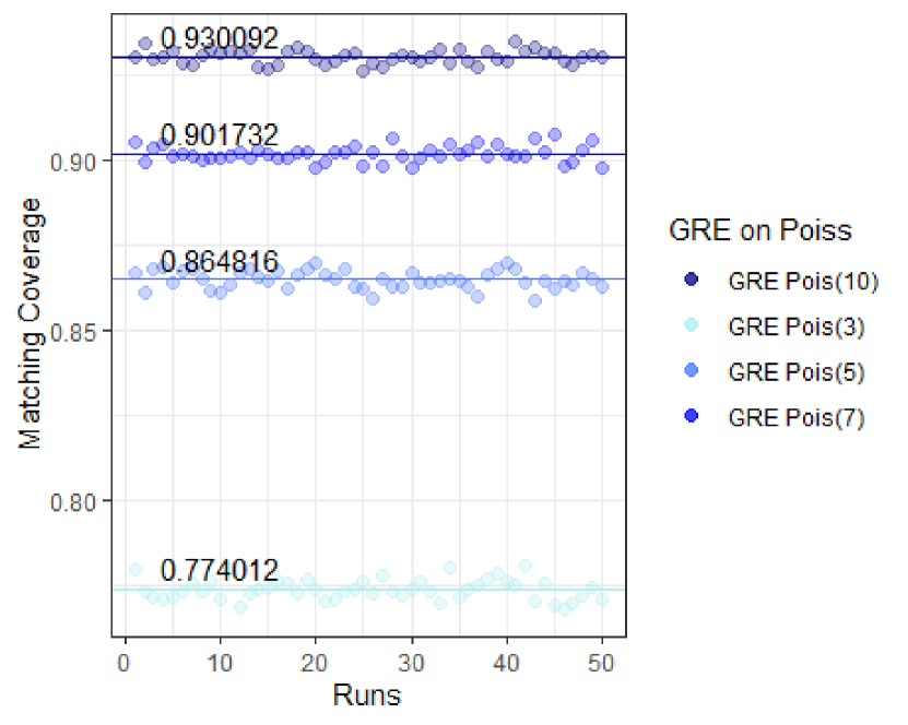
(a) Greedy on Poisson Laws

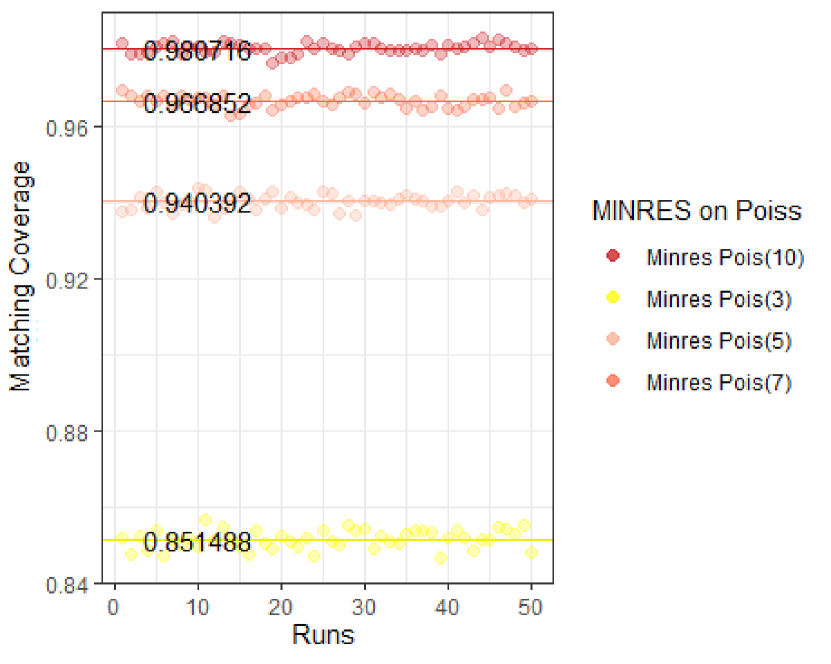
(b) Minres on Poisson Laws

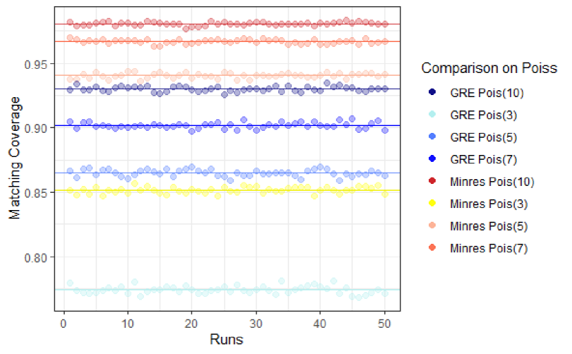
(c) Comparison on Poisson Law

Figure 13. Performance on Poisson Degree Distribution

Regular bipartite graphs.

We now address various degree distributions that correspond to regular bipartite graphs: each node has the same degree, in other words we have $\xi^{+}=\xi^{-}=\delta_{p}$, for some $p\in{\mathbb{N}}^{*}$, thereby generalizing the study of Sub-section 7.1. Notice that such bipartite graphs always admit a perfect matching. The distributions of matching coverage are given in Figures 14(a), 14(b) and 14(c).

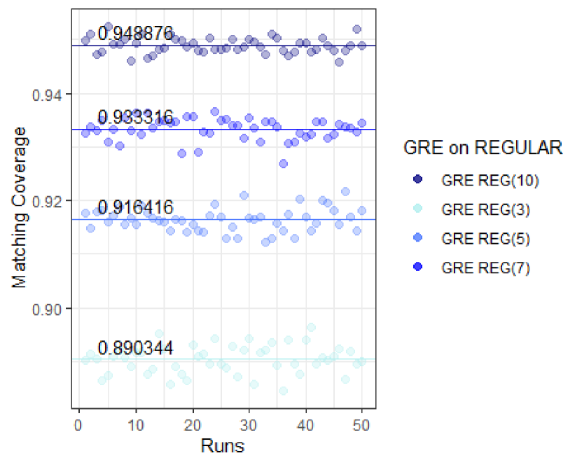
(a) Greedy on Regular Degree Distr.

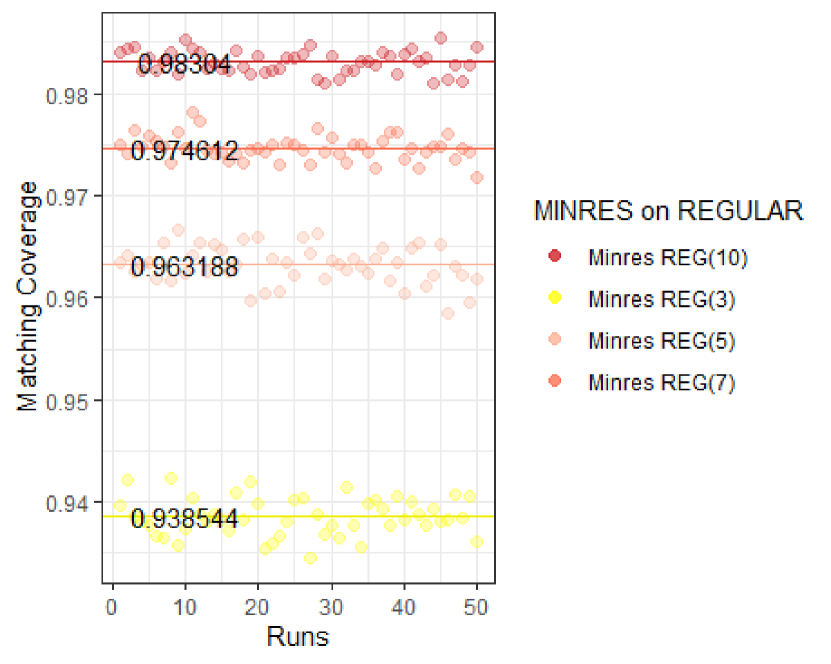
(b) Minres on Regular Degree Distr.

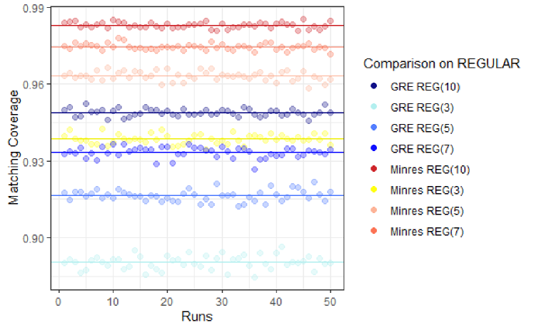
(c) Comparison on Regular Distribution

Figure 14. Performance on Regular Degree Distr.

These results illustrate well the increase of the performance of both algorithms, as the degree increase. For each designated distribution, we can also confirm that the matching coverage of Minres is consistently larger than that of Greedy.

Comparing the sub-figures of Figure 13 with the corresponding sub-figures of Figure 14, for the same average degree, we make the two following observations: First, both algorithms consistently perform better on regular graphs than on graphs with Poisson degree distributions, and the same mean. We conjecture that this phenomenon is due to the variance of Poisson degrees in the first panel: by restricting choices, the optimal partners for certain nodes (which we are trying to reach) might get blocked, while regular distributions provide more latitude to chose a match without missing an optimal one. Second, for both algorithms the distributions of matching coverage are more spread on regular graphs than on graphs having Poisson degrees. It seems that a uniform initial degree distribution provides more opportunities to deflect from typical runs, while the variance of degrees more often restricts the choices, creating a disparity between nodes.

7.3. On the optimal Algorithm of Karp, Vazirani and Vazirani

In [23], Karp, Vazirani and Vazirani present a different approach for online bipartite matchings on graphs. The authors define online algorithms as a way of picking the matches of “girls” (i.e., nodes on the ‘+’ side) that arrive one by one, based only on the identity of their neighbors on the ‘boys’ side (i.e., the ‘-’ side). By working with the adjacency matrix of the graph, it means that the columns are revealed one by one and the match is processed upon knowing the information of the current column. Our approach based on local algorithms, is a bit different, and actually use more information. Indeed, we also consider the degree of each neighbor of the incoming ‘girl’, and the neighbors of its match of her ’boy’ neighbor.

Second, the performance metrics considered in [23] is the so-called adversary approach. It allows to get a lower bound on the performance of online algorithms, as defined above. Namely, Theorem 2 in [23] states that in that context, the matching coverage is at least $1-1/e-{o(n)/n}$. This also happens to be the expected matching coverage for the Random algorithm defined therein (which is roughly equivalent to our Greedy). In the present work, we are interested in a different metrics: we establish convergence to a deterministic value of the average matching ratio, rather than a lower bound.

So it is clear that our framework differ with that of [23]. However, to gain some insights on how our algorithms based on the degree distribution stand against their counterparts on real graphs, we conducted the following study: we let $G$ be a randomly generated graph with 5000 nodes, from an upper triangular adjacency matrix that is specified as follows: all diagonal elements are 1, thereby insuring the existence of a perfect matching, and all upper elements are Bernoulli($p$) random variables, where $p$ is so that the graph has average degree, say, $5$. Such graphs provide the worst case scenarios for the framework in [23]. Then, on the graph $G$ we run the exploration algorithms (Section 3) for both Greedy and Minres. In parallel, we extract the degree distributions $(\mathbf{d}^{+},\mathbf{d}^{-})$ of the graph under consideration, on which we run both algorithms Greedy and Minres (joint construction of Section 4), thereby constructing another (multi-)graph having the same degree distribution. Our results can be summarized in Figure 15.

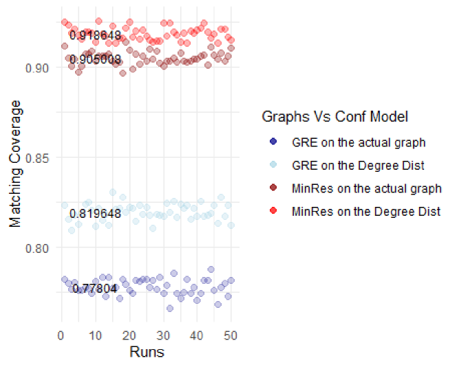
Figure 15. Exploration Vs Conf Model

Figure 15 shows that matching algorithms that are jointly constructed with the CM achieve a better matching coverage than on this particular graph. In other words, matching algorithms typically perform badly on this particular graph, with respect to a graph that is obtained as a uniform draw amongst graphs having the same degree distribution, unsurprisingly hinting at the influence of the graph topology on the considered matching algorithms. Simulations indicate that this influence is enhanced in Minres with respect to Greedy. Last, we observe again that Minres produces a better matching coverage than Greedy in all cases.

7.4. Notes and Conclusion

In this work, we introduced a procedure to approximate the matching coverage of local matching algorithms on graphs, using the hydrodynamic limit, in the large graph asymptotics, of a measure-valued Markov process representing the joint construction of the matching together with the graph itself, as a realization of the bipartite configuration model.

Transposing the matching algorithms into the dynamics of the residual degree distributions of the considered graphs, allowed us to predict the results of the considered algorithms, with a remarkable accuracy. This results in a dramatic reduction of the problem complexity: as long as one is interested in the matching coverage of the algorithm under consideration, one only needs to keep track of the residual degree distribution, and not of the whole graph geometry.

As our simulations indicate, two natural and interesting problems arise: The first (and probably hardest) one is to quantify the influence of the graph topology on the average matching coverage, for a given algorithm. The second concerns the optimality of Minres. Indeed, among all local algorithms we addressed, Minres always leads to better results. Is this criterion optimal for the matching coverage, and if so, in what probabilistic sense, and among which class of algorithms? Building on these two problems, we believe that the present work opens a promising line of research on the topic.

References

- [1] Paola Bermolen, Matthieu Jonckheere, Federico Larroca, and Pascal Moyal. Estimating the transmission probability in wireless networks with configuration models. ACM Transactions on Modeling and Performance Evaluation of Computing Systems (TOMPECS), 1(2):1–23, 2016.
- [2] Paola Bermolen, Matthieu Jonckheere, Federico Larroca, and Manuel Saenz. Degree-greedy algorithms on large random graphs. ACM SIGMETRICS Performance Evaluation Review, 46(3):27–32, 2019.
- [3] Paola Bermolen, Matthieu Jonckheere, and Pascal Moyal. The jamming constant of uniform random graphs. Stochastic Processes and their Applications, 127(7):2138–2178, 2017.
- [4] Patrick Billingsley. Convergence of probability measures. John Wiley & Sons, 2013.
- [5] Béla Bollobás and Bollobás Béla. Random graphs. Number 73. Cambridge university press, 2001.
- [6] Allan Borodin, Calum MacRury, and Akash Rakheja. Bipartite stochastic matching: Online, random order, and iid models. arXiv preprint arXiv:2004.14304, 2020.
- [7] Graham Brightwell, Svante Janson, and Malwina Luczak. The greedy independent set in a random graph with given degrees. Random Structures & Algorithms, 51(4):565–586, 2017.
- [8] Richard A Brualdi, Frank Harary, and Zevi Miller. Bigraphs versus digraphs via matrices. Journal of Graph Theory, 4(1):51–73, 1980.
- [9] Brian Brubach, Nathaniel Grammel, Will Ma, and Aravind Srinivasan. Follow your star: New frameworks for online stochastic matching with known and unknown patience. In International Conference on Artificial Intelligence and Statistics, pages 2872–2880. PMLR, 2021.
- [10] Jianer Chen, Qin Huang, Iyad Kanj, and Ge Xia. Optimal streaming algorithms for graph matching. arXiv preprint arXiv:2102.06939, 2021.
- [11] Ningyuan Chen and Mariana Olvera-Cravioto. Directed random graphs with given degree distributions. Stochastic Systems, 3(1):147 – 186, 2013.
- [12] Laurent Decreusefond, Jean-Stéphane Dhersin, Pascal Moyal, and Viet Chi Tran. Large graph limit for an SIR process in random network with heterogeneous connectivity. Annals of Applied Probability, 22(2):541–575, 04 2012.
- [13] Laurent Decreusefond and Pascal Moyal. Fluid limit of a heavily loaded edf queue with impatient customers. Markov Processes and Related Fields, 14:131–157, 2008.
- [14] Laurent Decreusefond and Pascal Moyal. A functional central limit theorem for the M/GI/ queue. Annals of Applied Probability, 18(6):2156–2178, 2008.
- [15] Bogdan Doytchinov, John Lehoczky, and Steven Shreve. Real-time queues in heavy traffic with earliest-deadline-first queue discipline. Annals of Applied Probability, pages 332–378, 2001.
- [16] Jack Edmonds. Paths, trees, and flowers. Canadian Journal of Mathematics, 17:449–467, 1965.
- [17] Alireza Farhadi, Mohammad Taghi Hajiaghayi, Tung Mah, Anup Rao, and Ryan A Rossi. Approximate maximum matching in random streams. In Proceedings of the Fourteenth Annual ACM-SIAM Symposium on Discrete Algorithms, pages 1773–1785. SIAM, 2020.
- [18] Jon Feldman, Aranyak Mehta, Vahab Mirrokni, and Shan Muthukrishnan. Online stochastic matching: Beating 1-1/e. In 2009 50th Annual IEEE Symposium on Foundations of Computer Science, pages 117–126. IEEE, 2009.
- [19] David Gamarnik and David A Goldberg. Randomized greedy algorithms for independent sets and matchings in regular graphs: Exact results and finite girth corrections. Combinatorics, Probability and Computing, 19(1):61–85, 2010.
- [20] Gagan Goel and Aranyak Mehta. Online budgeted matching in random input models with applications to adwords. In SODA, volume 8, pages 982–991, 2008.
- [21] H Christian Gromoll, Amber L Puha, and Ruth J Williams. The fluid limit of a heavily loaded processor sharing queue. Annals of Applied Probability, 12(3):797–859, 2002.
- [22] Remco van der Hofstad. Random Graphs and Complex Networks, volume 1 of Cambridge Series in Statistical and Probabilistic Mathematics. Cambridge University Press, 2016.
- [23] R. M. Karp, U. V. Vazirani, and V. V. Vazirani. An optimal algorithm for on-line bipartite matching. In Proceedings of the Twenty-Second Annual ACM Symposium on Theory of Computing, STOC ’90, page 352–358, New York, NY, USA, 1990. Association for Computing Machinery.
- [24] Haya Kaspi and Kavita Ramanan. Law of large numbers limits for many-server queues. Annals of Applied Probability, 21(1):33–114, 2011.
- [25] Mohammad Mahdian and Qiqi Yan. Online bipartite matching with random arrivals: An approach based on strongly factor-revealing lps. In Proceedings of the Forty-Third Annual ACM Symposium on Theory of Computing, STOC ’11, page 597–606, New York, NY, USA, 2011. Association for Computing Machinery.
- [26] Michael Molloy, Bruce Reed, Mark Newman, Albert-László Barabási, and Duncan J Watts. A critical point for random graphs with a given degree sequence. In The Structure and Dynamics of Networks, pages 240–258. Princeton University Press, 2011.
- [27] Mark Newman. Networks. Oxford university press, 2018.
- [28] Sumedh Tirodkar. Deterministic Algorithms for Maximum Matching on General Graphs in the Semi-Streaming Model. In Sumit Ganguly and Paritosh Pandya, editors, 38th IARCS Annual Conference on Foundations of Software Technology and Theoretical Computer Science (FSTTCS 2018), volume 122 of Leibniz International Proceedings in Informatics (LIPIcs), pages 39:1–39:16, Dagstuhl, Germany, 2018. Schloss Dagstuhl–Leibniz-Zentrum fur Informatik.
- [29] Nicholas C. Wormald. The differential equation method for random graph processes and greedy algorithms. Lectures on approximation and randomized algorithms, 73:155, 1999.