Explicit Rate-Optimal Streaming Codes
with Smaller Field Size

Abstract

Streaming codes are a class of packet-level erasure codes that ensure packet recovery over a sliding window channel which allows either a burst erasure of size $b$ or $a$ random erasures within any window of size $(\tau+1)$ time units, under a strict decoding-delay constraint $\tau$. The field size over which streaming codes are constructed is an important factor determining the complexity of implementation. The best known explicit rate-optimal streaming code requires a field size of $q^{2}$ where $q\geq\tau+b-a$ is a prime power. In this work, we present an explicit rate-optimal streaming code, for all possible $\{a,b,\tau\}$ parameters, over a field of size $q^{2}$ for prime power $q\geq\tau$. This is the smallest-known field size of a general explicit rate-optimal construction that covers all $\{a,b,\tau\}$ parameter sets. We achieve this by modifying the non-explicit code construction due to Krishnan et al. to make it explicit, without change in field size.

I Introduction

Enabling low-latency reliable communication for applications such as telesurgery, industrial automation, augmented reality and vehicular communication is a key target of 5G communication systems. For instance, telesurgery camera flow requires packet-loss rate less than $10^{-3}$ and end-to-end latency below $150$ ms [1]. To combat the packet drops that are an inevitable part of any communication network, one approach is to employ feedback-based methods such as ARQ. But such feedback-based schemes incur round-trip propagation delay, making it difficult to meet low-latency requirements. Blind re-transmission of packets is another option, but is inefficient as it amounts to using a repetition code. Streaming codes are a class of packet-level erasure codes and represent a natural way of achieving reliable, low-latency communication at the packet level.

A packet-expansion encoding framework for streaming codes was introduced in [2]. Given message packet at time $t$ denoted by $\underline{u}(t)\in\mathbb{F}_{q}^{k}$, the coded packet $\underline{x}(t)\in\mathbb{F}_{q}^{n}$, at time $t$, is generated by appending parity packet $\underline{p}(t)\in\mathbb{F}_{q}^{n-k}$ to $\underline{x}(t)$. More formally, $\underline{x}(t)=\left[\underline{u}(t)^{T}\ \underline{p}(t)^{T}\right]^{T}$. The encoder is causal and hence $\underline{p}(t)$ depends only on $\underline{u}(t)$ and prior message packets. In [2, 3], streaming codes that can handle burst erasure of size $b$ under a decoding-delay constraint $\tau$ are presented. The decoding-delay constraint $\tau$ means that for recovery of message packet $\underline{u}(t)$ only packets with index $\leq t+\tau$ can be accessed. In [4], Badr et al. presented a delay constrained sliding window (DCSW) channel model that allows burst or random erasures. This channel can be viewed as a deterministic approximation of the Gilbert-Elliot channel [5]. In the DCSW channel model, within any sliding window of size $w$ time units, either a burst erasure of length $\leq b$ or else, at most $a$ random erasures can occur. Additionally there is a decoding-delay constraint $\tau$. This model is non-trivial only if $0<a\leq b\leq\tau$. As it turns out, we can, without loss in generality, set $w=\tau+1$ (see [6]). Thus the DCSW channel is parameterized by the three-parameter set $\{a,b,\tau\}$. An $(a,b,\tau)$ streaming code is a packet-level code that can recover from all the permissible erasure patterns of an $\{a,b,\tau\}$ DCSW channel, within decoding-delay $\tau$. Some other models of erasure codes for streaming can be found in [7, 8, 9, 10].

In [4] an upper bound on the rate of an $(a,b,\tau)$ streaming code was presented and it was later shown in [11, 12] that this rate is achievable for all possible $\{a,b,\tau\}$ parameters. It follows from these results that the optimal rate of $(a,b,\tau)$ streaming code is given by $R_{\text{opt}}=\frac{\tau+1-a}{\tau+1-a+b}$. The rate-optimal codes presented in [11, 12] required a finite field alphabet that is exponential in $\tau$. A non-explicit rate-optimal streaming code, which requires a field $\mathbb{F}_{q^{2}}$ with prime power $q\geq\tau$, is presented in [6]. Subsequently, an explicit construction was presented in [13] requiring field size $q^{2}$, for $q\geq\tau+b-a$, a prime power. Streaming codes for variable packet sizes are explored in [14]. Explicit rate-optimal constructions having linear field size for some $\{a,b,\tau\}$ parameter ranges are presented in [6, 15, 16]. However, the construction in [13] remains the smallest field size explicit rate-optimal streaming code construction that exists for all possible $\{a,b,\tau\}$. Note that the field size required for the explicit code construction in [13] is larger than the field size $q^{2}\geq\tau^{2}$ requirement of the code in [6]. In the present paper, we present an explicit rate-optimal code having the same field-size requirement $q^{2}$, with prime power $q\geq\tau$, as that of the non-explicit code in [6]. Smaller field size constructions simplify implementation and are hence of significant, practical interest.

The principal contribution of the paper is thus an explicit rate-optimal streaming code construction for all possible $\{a,b,\tau\}$ parameters. The construction is motivated by the structure of the non-explicit code in [6] and has smallest known field size of an explicit rate-optimal streaming code construction that holds for all $\{a,b,\tau\}$ parameters.

Section II presents the diagonal-embedding framework for embedding a scalar code within the packet stream. The explicit construction of the scalar code having field size $q^{2}\geq\tau^{2}$ is presented in Section III. Proof that this construction, in conjunction with diagonal embedding, results in a rate-optimal streaming code is presented in Section IV.

We use $[a:b]$ to denote the set $\{a,a+1,\dots,b-1,b\}$. Given a $(k\times n)$ matrix $M$, $I\subseteq[0:k-1]$ and $J\subseteq[0:n-1]$, $M(I,J)$ will denote the sub-matrix of $M$ comprised of rows with row-index in $I$ and columns with column-index in $J$. We use $|M|$ to denote the determinant of $M$, $I_{u}$ denotes $(u\times u)$ identity matrix and $\underbrace{\mathbf{0}}_{(u\times v)}$ will denote the $(u\times v)$ all-zero matrix.

II Preliminaries

II-A Diagonal Embedding

Diagonal embedding, introduced in [3], can be viewed as a framework for deriving a packet-level code from a scalar code. This technique has been consistently used in the streaming-code literature. Let $\mathcal{C}$ be an $[n,k]$ scalar code in systematic form, with first $k$ code symbols being message symbols. Consider a packet-level code with coded packet at time $t$ denoted by $\underline{x}(t)=[x_{0}(t)~{}x_{1}(t)\dots x_{n-1}(t)]^{T}$. We will say that the packet-level code is obtained by diagonal embedding of the scalar code $\mathcal{C}$ if for all $t$, each $n$-tuple $\left(x_{0}(t),x_{1}(t+1),\dots,x_{n-1}(t+n-1)\right)$ is a codeword in the scalar code $\mathcal{C}$. The packet-level code shares the rate $\frac{k}{n}$ of the underlying scalar code. Diagonal embedding is illustrated in Fig.1.

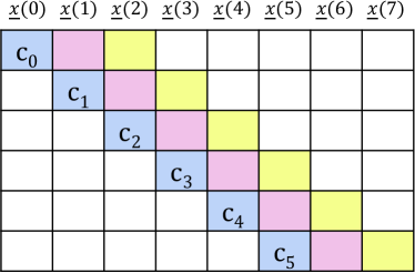
Figure 1: Packet-level code constructed by diagonal embedding of a scalar code of block length $6$. Here each column indicates a coded packet.

II-B Properties Required of the Scalar Code

Let $\delta=b-a$. In order to show that the packet-level code constructed through diagonal embedding of an $[n=\tau+1+\delta,k=n-b]$ scalar code $\mathcal{C}$ is a rate-optimal $(a,b,\tau)$ streaming code it suffices to show that the following erasure recovery properties hold for codeword $(c_{0},c_{1},\dots,c_{n-1})\in\mathcal{C}$ that occupies the time indices $0\leq t\leq(n-1)$. Analogous, time-shifted versions of these below conditions apply to the other embedded codewords (see [6] for details).

1. Any code symbol $c_{t}$ with $t\in[0:\delta-1]$ should be recoverable from the erasure of a burst of $b$ packets, corresponding to time indices in $[t:t+b-1]$, by accessing non-erased code symbols in the set $\{c_{i}\mid t<i\leq\tau+t\}\cup\{c_{i}\mid i<t\}$. The latter set represents previously-decoded code symbols.

2. Any code symbol $c_{t}$ with $t\in[0:\delta-1]$ should be recoverable from any $a$ random packet erasures, corresponding to time indices $t$ and $(a-1)$ indices in $[t+1:\tau+t]$, by accessing non-erased code symbols in the set $\{c_{i}\mid t<i\leq\tau+t\}\cup\{c_{i}\mid i<t\}$.

3. For any $t\in[\delta:\tau+1-a]$, code symbols $\{c_{i}\mid i\in[t:t+b-1]\}$ should be recoverable by accessing remaining code symbols $\{c_{i}\mid i\notin[t:t+b-1]\}$.

4. For any set $A\subseteq[\delta:\tau+\delta]$ with $|A|=a$, code symbols $\{c_{i}\mid i\in A\}$ should be recoverable by accessing the remaining code symbols $\{c_{i}\mid i\notin A\}$.

It follows from B2 property for $t=\tau+1-a$ that the last $n-k=b$ code symbols $\{c_{k},\dots,c_{n-1}\}$ can be computed from the first $k$ code symbols $\{c_{0},\dots,c_{k-1}\}$, thereby guaranteeing systematic encoding with $\{c_{0},\dots,c_{k-1}\}$ as message symbols.

III Scalar Code Construction

Our explicit, rate-optimal streaming code construction will employ diagonal embedding as well as an $[n=\tau+1+\delta,k=n-b]$ scalar code satisfying the four erasure recovery properties listed above in Section II. We begin by recursively defining a matrix that will be used to specify the parity-check matrix of our scalar code. This recursive definition can be viewed as an extension of the recursive matrix definition in [17] that was used to construct rate-optimal binary streaming codes for the situation when only burst erasures are present.

Definition 1.

For any positive integers $u,v$ and $a$, we recursively define the $(u\times v)$ matrix $\mathbf{P}_{u,v}^{a}$ as shown below:

$$\mathbf{P}_{u,v}^{a} = \begin{cases}\left[\begin{array}[]{ccc}I_{u}&\underbrace{\mathbf{0}}_{(u\times a)}&\mathbf{P}_{u,v-u-a}^{a}\end{array}\right]&u+a<v\\ \ \\ \left[\begin{array}[]{cc}I_{u}&\underbrace{\mathbf{0}}_{(u\times(v-u))}\end{array}\right]&u\leq v\leq u+a\\ \ \\ \left[\begin{array}[]{c}I_{v}\\ \mathbf{P}_{u-v,v}^{a}\end{array}\right]&v<u\\ \end{cases}$$

For example, $\mathbf{P}^{2}_{3,7}=[I_{3}~{}\underbrace{\mathbf{0}}_{(3\times 2)}~{}\mathbf{P}_{3,2}^{2}],~{}\mathbf{P}_{3,2}^{2}=\left[\begin{array}[]{c}I_{2}\\ \mathbf{P}_{1,2}^{2}\end{array}\right]~{}\text{and}~{}\mathbf{P}_{1,2}^{2}=[1~{}0]$. Therefore we have

$$\mathbf{P}^{2}_{3,7}=\left[\begin{array}[]{ccc|cc|cc}1&0&0&0&0&1&0\\ 0&1&0&0&0&0&1\\ \cline{6-7}\cr 0&0&1&0&0&1&0\end{array}\right].$$

Construction 1.

Let $\delta=b-a$, $q\geq\tau$ be a prime power and $\alpha\in\mathbb{F}_{q^{2}}\setminus\mathbb{F}_{q}$. Let the $(a\times(\tau+1-a))$ matrix $\mathbf{C}$ over $\mathbb{F}_{q}$ be such that any square sub-matrix of it is non-singular. We define an $[n=\tau+1+\delta,k=n-b]$ scalar code having a parity check matrix $H$ that is defined in step-by-step fashion below:

• initialize $H$ to be the $(b\times(\tau+1+\delta))$ all-zero matrix,

• set $H([0:\delta-1],[0:\delta-1])\ =\ \alpha I_{\delta}$,

• set $H([0:\delta-1],[b:\tau-1])\ =\ \mathbf{P}^{a}_{\delta,\tau-b}$,

• set $H([\delta:b-1],[0:a-1])\ =\ I_{a}$,

• set $H([\delta:b-1],[a:\tau])\ =\ \mathbf{C}$,

• set $H(0,\tau)=\alpha$ and $H([1:\delta],[\tau+1:\tau+\delta])=I_{\delta}$.

The first $\delta$ rows of the parity check matrix $H$ are given by:

$$H([0:\delta-1],[0:\tau+\delta])$$

$$=\left[\begin{array}[]{cccc|c|c|ccccc}\alpha&&&&\hbox{\multirowsetup$\underbrace{\mathbf{0}}_{(\delta\times a)}$}&\hbox{\multirowsetup$\underbrace{\mathbf{P}_{\delta,\tau-b}^{a}}_{(\delta\times(\tau-b))}$}&\alpha&&&&0\\ &\alpha&&&&&&1&&&0\\ &&\ddots&&&&&&\ddots&&\vdots\\ &&&\alpha&&&&&&1&0\end{array}\right],$$

and the last $(b-\delta)=a$ rows of $H$ by:

$$H([\delta:b-1],[0:\tau+\delta])$$

$$=\left[\begin{array}[]{cccc|c|c|c}1&&&&\hbox{\multirowsetup$\underbrace{\mathbf{C}}_{(a\times(\tau+1-a))}$}&\hbox{\multirowsetup$\underbrace{\mathbf{0}}_{(a\times(\delta-1))}$}&1\\ &1&&&&&0\\ &&\ddots&&&&\vdots\\ &&&1&&&0\end{array}\right].$$

As defined above, $H([\delta:b-1],[0:\tau])$ is the parity check matrix of a $[\tau+1,\tau+1-a]$ MDS code. A finite field of size $q\geq\tau$ suffices to explicitly construct the matrix $\mathbf{C}$. It can be verified that the last $a$ rows of $H$ are the same as that of the non-explicit code presented in [6].

III-A Example Constructions

III-A1 $(a=2,b=5,\tau=12)$

Here $\delta=3$, $\tau-b=7$, $\tau+1-a=11$ and $\tau+1+\delta=16$. The parity check matrix $H$ of $[n=16,k=11]$ scalar code is given in this case by:

$$\left[\begin{array}[]{ccc|cc|ccccccc|cccc}\alpha&0&0&0&0&1&0&0&0&0&1&0&\alpha&0&0&0\\ 0&\alpha&0&0&0&0&1&0&0&0&0&1&0&1&0&0\\ 0&0&\alpha&0&0&0&0&1&0&0&1&0&0&0&1&0\\ \hline\cr 1&0&\vrule\lx@intercol\hfil\hbox{\multirowsetup$\underbrace{\mathbf{C}}_{(2\times 11)}$}\hfil\lx@intercol\vrule\lx@intercol&0&0&1\\ 0&1&\vrule\lx@intercol\hfil\hfil\lx@intercol\vrule\lx@intercol&0&0&0\end{array}\right].$$

III-A2 $(a=3,b=6,\tau=8)$

Here $\delta=3$, $\tau-b=2$, $\tau+1-a=6$ and $\tau+1+\delta=12$. The parity check matrix $H$ of $[n=12,k=6]$ scalar code is given in this case by:

$$\left[\begin{array}[]{ccc|ccc|cc|cccc}\alpha&0&0&0&0&0&1&0&\alpha&0&0&0\\ 0&\alpha&0&0&0&0&0&1&0&1&0&0\\ 0&0&\alpha&0&0&0&1&0&0&0&1&0\\ \hline\cr 1&0&0&\lx@intercol\hfil\hbox{\multirowsetup$\underbrace{\mathbf{C}}_{(3\times 6)}$}\hfil\lx@intercol\vrule\lx@intercol&0&0&1\\ 0&1&0&\vrule\lx@intercol\hfil\hfil\lx@intercol\vrule\lx@intercol&0&0&0\\ 0&0&1&\vrule\lx@intercol\hfil\hfil\lx@intercol\vrule\lx@intercol&0&0&0\end{array}\right].$$

IV Proof of Erasure Recovery Properties

In this section we show that the $[n=\tau+1+\delta,k=n-b]$ scalar code defined in Section III satisfies all the four erasure recovery conditions. This will in turn prove that the packet-level code obtained by diagonal embedding of this scalar code is a rate-optimal $(a,b,\tau)$ streaming code. This $(a,b,\tau)$ streaming code can be explicitly constructed over a finite field of size $q^{2}\geq\tau^{2}$.

It can be proved that the scalar code satisfies R1 and R2 properties using arguments similar to that presented in [6]. Nevertheless for the sake of completeness, we provide proof of all the four properties here.

IV-A Proof of B1 Property

Property B1 is verified by showing that for every $t\in[0:\delta-1]$, there exists a parity check equation having support at $t$ and zeros at indices $[t+1:t+b-1]\cup[t+\tau+1:\tau+\delta]$. Using this parity-check equation, code symbol $c_{t}$ can be recovered from a burst erasure confined to $[t:t+b-1]$ by accessing only the non-erased code symbols having index $\leq t+\tau$.

For the $(a=2,b=5,\tau=12)$ example, suppose symbols $\{c_{0},c_{1},c_{2},c_{3},c_{4}\}$ are erased. Row $0$ of the parity check matrix $H$ for this example is as shown below:

$$\left(\begin{array}[]{cccccccccccccccc}\alpha&0&0&0&0&1&0&0&0&0&1&0&\alpha&0&0&0\end{array}\right).$$

It follows that $\alpha c_{0}+c_{5}+c_{10}+\alpha c_{12}=0$. Hence $c_{0}$ can be recovered by accessing symbols till $c_{12}$. Now for the $(a=3,b=6,\tau=8)$ example, consider a burst erasure such that $\{c_{2},c_{3},c_{4},c_{5},c_{6},c_{7}\}$ are lost. It follows from row $2$ of $H$ that $\alpha c_{2}+c_{6}+c_{10}=0$, but since $c_{6}$ is erased this equation alone is not sufficient to recover $c_{2}$. We get $\alpha c_{0}+c_{6}+\alpha c_{8}=0$ from the $0$-th row of $H$. From these two parity-check equations we obtain $\alpha c_{2}+c_{10}-\alpha c_{0}-\alpha c_{8}=0$, using which $c_{2}$ can be recovered by accessing code symbols till $c_{10}$. We now prove the B1 property for general $\{a,b,\tau\}$. We use the notation $h(t)$ to denote the $t$-th row of $H$. The symbol ’X’ is used as a don’t care symbol in the arguments below.

IV-A1 $\tau-b\geq\delta$

From the definition of the matrix $P_{\delta,\tau-b}^{a}$, the first $\delta$ columns of $P_{\delta,\tau-b}^{a}$ form $I_{\delta}$. The $t$-th row of $H$ looks as shown below:

$$\begin{array}[]{ccccccccccccccccccc}0&&&t&&&&t+b&&&&b+\delta&&\tau+t&&&\tau+\delta\\ (0&\cdots&0&\alpha&0&\cdots&0&1&0&\cdots&0&X&\cdots&X&0&\cdots&0)\end{array}$$

Therefore, using the parity check equation given by $h(t)$ we can recover code symbol $c_{t}$ from a burst erasures at $[t:t+b-1]$ by accessing available code symbols with index $\leq\tau+t$.

IV-A2 $\tau-b<\delta$

Let $\ell=\tau-b$, $\delta=v\ell+x$ where $0\leq x<\ell$. Then by definition $P_{\delta,\ell}^{a}=\left[I_{\ell}~{}\cdots~{}I_{\ell}~{}{P_{x,\ell}^{a}}^{T}\right]^{T}.$ We further divide the proof of this case into three sub-cases.

$t\in[0:\ell-1]$

In this case, the $t$-th row of $H$ satisfies the requirement as shown below and hence can be used for recovery of $c_{t}$.

$$\begin{array}[]{cccccccccccccccc}0&&&t&&&&t+b&&&&\tau+t&&&\tau+\delta\\ (0&\cdots&0&\alpha&0&\cdots&0&1&0&\cdots&0&X&0&\cdots&0)\end{array}$$

$t\in[\ell:v\ell-1]$

Let $t=v^{\prime}\ell+x^{\prime}$ where $1\leq v^{\prime}\leq v-1$ and $0\leq x^{\prime}<\ell$. The $t$-th row $h(t)$ is of the form:

$$\begin{array}[]{ccccccccccccccccc}0&&&t&&&&b+x^{\prime}&&&&\tau+t&&&\tau+\delta\\ (0&\cdots&0&\alpha&0&\cdots&0&1&0&\cdots&0&X&0&\cdots&0)\end{array}$$

This parity check equation does not have $(b-1)$ zeros following the index $t$. Therefore we look at the equation given by $(t-\ell)$-th row of $H$:

$$\begin{array}[]{ccccccccccccccccc}0&&&t-\ell&&&&b+x^{\prime}&&&&\tau+t-\ell&&&\tau+\delta\\ (0&\cdots&0&\alpha&0&\cdots&0&1&0&\cdots&0&X&0&\cdots&0)\end{array}$$

Thus we get a parity check $h(t)-h(t-\ell)$ as shown below:

$$\begin{array}[]{ccccccccccccccccc}0&&&t&&&&\tau+t-\ell&&&&\tau+t&&&\tau+\delta\\ (X&\cdots&X&\alpha&0&\cdots&0&X&0&\cdots&0&X&0&\cdots&0)\end{array}$$

Note that $\tau+t-\ell=(\tau+t)-(\tau-b)=t+b$. Therefore there are $(b-1)$ zeros following index $t$ in the parity check equation shown above and this parity check equation can be used to recover code symbol $c_{t}$.

$t\in[v\ell:v\ell+x-1]$

Let $t=v\ell+x^{\prime}$, where $x^{\prime}\leq x-1$. The $t$-th parity check equation $h(t)$ is of the form:

$$\begin{array}[]{cccccccccccccccccccc}0&&&t&&&&b+x^{\prime}&&&&\tau&&&\tau+t&&&\tau+\delta\\ (0&\cdots&0&\alpha&0&\cdots&0&1&X&\cdots&X&0&\cdots&0&X&0&\cdots&0)\end{array}$$

as the first $x$ columns of $P_{x,\ell}^{a}$ are given by $I_{x}$. Let $y_{i}=(v-1)\ell+i-b$. For any $i\in[b+x^{\prime}:\tau-1]$, $h(y_{i})$ is as shown below:

$$\begin{array}[]{cccccccccccccccccccc}0&&&y_{i}&&&&i&&&&\tau+y_{i}&&&\tau+\delta\\ (0&\cdots&0&\alpha&0&\cdots&0&1&0&\cdots&0&X&0&\cdots&0)\end{array}$$

Let $S\subseteq[0:\tau+\delta]$ be the support of $h(t)\cap[b+x^{\prime}:\tau-1]$. We now look at the parity check equation given by $h(t)-\sum\limits_{i\in S}h(y_{i})$. Clearly $y_{i}<t$ for all $i\in[b+x^{\prime}:\tau-1]$. It can be seen that the entries at indices $[b+x^{\prime}:\tau-1]$ of $h(t)$ are either $0$ or $1$. Hence $h(t)-\sum\limits_{i\in S}h(y_{i})$ takes the following form:

$$\begin{array}[]{ccccccccccccccccc}0&&&t&&&&\tau+(v-1)\ell+x^{\prime}&&&\tau+t&&&\tau+\delta\\ (X&\cdots&X&\alpha&0&\cdots&0&1&X&\cdots&X&0&\cdots&0)\end{array}$$

Note that $\tau+(v-1)\ell+x^{\prime}=\tau+t-\ell=t+b$. Thus there are $(b-1)$ zeros following index $t$ in the above equation. Therefore code symbol $c_{t}$ can be recovered by accessing code symbols with index $\leq\tau+t$.

IV-B Proof of Property R1

Let $H^{(t)}$ be the parity check matrix of the punctured code obtained by deleting coordinates $[t+\tau+1:n-1]$ from the scalar code and let $\underline{h}_{i}^{(t)}$ denote the $i-$th column of $H^{(t)}$, for $i\in[0:\tau+t]$. To prove $R1$ property, it is enough to show that $\underline{h}_{t}^{(t)}\notin span\langle\{\underline{h}_{i}^{(t)}\mid i\in A\}\rangle$ for any $A\subset[t+1:\tau+t]$ with $|A|=a-1$, for all $t\in[0:\delta-1]$.

IV-B1 $t=0$

In this case we need to look at $H^{(0)}$.

$$H^{(0)}=\left[\begin{array}[]{c|ccccc}\alpha&X&\cdots&\cdots&X&\alpha\\ \hline\cr 0&\lx@intercol\hfil\hbox{\multirowsetup$I_{(a-1)}$}\hfil\lx@intercol&\lx@intercol\hfil\hbox{\multirowsetup$\underbrace{\mathbf{C}}_{((a-1)\times(\tau+1-a))}$}\hfil\lx@intercol\\ \vdots&&&&\\ 0&&&&&\end{array}\right].$$

Note that the last $(a-1)$ rows of $\underline{h}_{0}^{(0)}$ is all-zero. We also note that $H^{(0)}([1:a-1],[1:\tau])$ is the parity check matrix of an $[\tau,\tau+1-a]$ MDS code. Hence, it is not possible for any other $(a-1)$ columns of $H^{(0)}$ to linearly combine to obtain these $(a-1)$ zero entires, thus proving recoverability of $c_{0}$.

IV-B2 $t\in[1:\delta-1]$

Here look at the $(a\times(\tau+1))$ matrix $\hat{H}_{t}=H(\{t\}\cup[\delta+1:b-1],[t:\tau+t])$ which is a sub-matrix of $H^{(t)}$. Consider any $A\subseteq[1:\tau]$ with $|A|=a-1$. To prove $R1$ property it is sufficient to show that $0-$th column of $\hat{H}_{t}$ doesn’t lie in the linear span of columns of $\hat{H}_{t}$ indexed by $A$.

$$\hat{H}_{t}=\left[\begin{array}[]{c ccccc}\alpha&X&\cdots&\cdots&X&1\\ \hline\cr&\lx@intercol\hfil\hbox{\multirowsetup$H([\delta+1:b-1],[t:\tau])$}\hfil\lx@intercol&\lx@intercol\hfil\hbox{\multirowsetup$\underbrace{\mathbf{0}}_{((a-1)\times t)}$}\hfil\lx@intercol\\ &&&&\\ &&&&&\end{array}\right],$$

where $X$ is either $0$ or $1$. If $A\cap[\tau-t+1:\tau]\neq\phi$, then by MDS property the last $(a-1)$ entires of $0-$th column of $\hat{H}_{t}$ can not be obtained by linear combination of $\{\hat{H}_{t}([1:a-1],j)\mid j\in A\}$. Now consider $A\subseteq[1:\tau-t]$. Suppose $\hat{H}_{t}([0:a-1],0)=\sum_{j\in A}\beta_{j}\hat{H}_{t}([0:a-1],j)$ where $\beta_{j}\in\mathbb{F}_{q^{2}}$. It can be argued using MDS parity property of $C$ matrix that there exists a unique linear combination of $\{\hat{H}_{t}([1:a-1],j)\mid j\in A\}$ with all coefficients in $\mathbb{F}_{q}\setminus\{0\}$ that result in $\hat{H}_{t}([1:a-1],0)$. Hence, $\beta_{j}\in\mathbb{F}_{q}\setminus\{0\}$, for all $j\in A$. Note that $\hat{H}_{t}(0,j)\in\mathbb{F}_{q}$ for all $j\in[1:\tau]$, whereas $\hat{H}_{t}(0,0)=\alpha\in\mathbb{F}_{q^{2}}\setminus\mathbb{F}_{q}$. So, $\hat{H}_{t}(0,0)\neq\sum_{j\in A}\beta_{j}\hat{H}_{t}(0,j)$, which is a contradiction. Thus, $0-$th column of $\hat{H}_{t}$ doesn’t lie in span of columns in $A$.

IV-C Proof of Property B2

It is clear from the definition of the B2 property that in order to prove B2 property it suffices to show that the sub-matrix $H([0:b-1],[t:t+b-1])$ is invertible for any $t\in[\delta:\tau+1-a]$. Before describing the general proof for invertibility of $H([0:b-1],[t:t+b-1])$, we first present some examples which illustrate our arguments. For $(a=2,b=5,\tau=12)$, the sub-matrix $H([0:4],[3:7])$ is as shown below:

$$\left[\begin{array}[]{cc|ccc}0&0&1&0&0\\ 0&0&0&1&0\\ 0&0&0&0&1\\ \hline\cr c_{0,1}&c_{0,2}&c_{0,3}&c_{0,4}&c_{0,5}\\ c_{1,1}&c_{1,2}&c_{1,3}&c_{1,4}&c_{0,5}\end{array}\right],$$

where $c_{i,j}=H(\delta+i,a+j)$. This matrix is invertible since $\left[\begin{array}[]{cc}c_{0,1}&c_{0,2}\\ c_{1,1}&c_{1,2}\end{array}\right]$ is a $(2\times 2)$ sub-matrix of the parity check matrix of a $[13,11]$ MDS code. Now consider $H([0:4],[10:14])$ which has the following structure:

$$\left[\begin{array}[]{ccc|cc}1&0&\alpha&~{}0{}&~{}0{}\\ \hline\cr 0&1&0&~{}1{}&~{}0{}\\ 1&0&0&~{}0{}&~{}1{}\\ \hline\cr c_{0,8}&c_{0,9}&c_{0,10}&~{}0{}&~{}0{}\\ c_{1,8}&c_{1,9}&c_{1,10}&~{}0{}&~{}0{}\end{array}\right].$$

The above matrix is non-singular if $M=\left[\begin{array}[]{ccc}1&0&\alpha\\ c_{0,8}&c_{0,9}&c_{0,10}\\ c_{1,8}&c_{1,9}&c_{1,10}\end{array}\right]$ has non-zero determinant. Clearly, $|M|=\begin{vmatrix}c_{0,9}&c_{0,10}\\ c_{1,9}&c_{1,10}\end{vmatrix}+\alpha\begin{vmatrix}c_{0,8}&c_{0,9}\\ c_{1,8}&c_{1,9}\end{vmatrix}$. Since $\begin{vmatrix}c_{0,9}&c_{0,10}\\ c_{1,9}&c_{1,10}\end{vmatrix}\in\mathbb{F}_{q}$, $\begin{vmatrix}c_{0,8}&c_{0,9}\\ c_{1,8}&c_{1,9}\end{vmatrix}\neq 0$ and $\alpha\in\mathbb{F}_{q^{2}}\setminus\mathbb{F}_{q}$, we have $|M|\neq 0$.

Now we move to the general proof of invertibility of $H([0:b-1],[t:t+b-1])$ for any $t\in[\delta:\tau+1-a]$. Since $H([\delta:b-1],[0:\tau])$ is the parity-check matrix of a $[\tau+1,\tau+1-a]$ MDS Code, any $(a\times a)$ sub-matrix of it is invertible. We will use this fact repeatedly in the proof given below. Let

$$\tau=vb+\ell~{}~{}~{}\text{where}~{}~{}~{}0\leq\ell<b.$$

Then $\tau+1-a=vb+\ell-a+1$. We divide the proof into multiple cases based on the range of value of $t$. In the below proof, we often ignore the sign of the determinant as it is irrelevant to invertibility of a matrix.

Case i) $t\in[\delta:(v-1)b]$

In this case $t+b-1\leq vb-1=\tau-\ell-1$. We note that

$$H([0:\delta-1],[\delta:vb-1])=\left[\begin{array}[]{c|c|c|c|c|c}\underbrace{\mathbf{0}}_{\delta\times a}&\hbox{\multirowsetup$~{}I_{\delta}~{}$}&\underbrace{\mathbf{0}}_{\delta\times a}&\hbox{\multirowsetup$\cdots$}&\hbox{\multirowsetup$~{}I_{\delta}~{}$}&\underbrace{\mathbf{0}}_{\delta\times a}\\ \end{array}\right].$$

From the structure of $H([0:\delta-1],[\delta:vb-1])$ given above it can be observed that $H([0:\delta-1],[t:t+b-1])$, for $t\in[\delta:(v-1)b]$, is composed of $a$ all-zero columns and $\delta$ columns from identity matrix. Let $t=xb+\theta$ where $\theta<b$.

Suppose $\theta\leq\delta-1$, then the sub-matrix $H([0:b-1],[t:t+b-1])$ is of the following form:

$$\left[\begin{array}[]{c|c|c}\hbox{\multirowsetup$\underbrace{\mathbf{0}}_{(\theta\times(\delta-\theta))}$}&\hbox{\multirowsetup~{}~{}~{}$\underbrace{\mathbf{0}}_{(\delta\times a)}$~{}~{}~{}}&\hbox{\multirowsetup$I_{\theta}$}\\ &&\\ \cline{1-1}\cr\cline{3-3}\cr\hbox{\multirowsetup$I_{(\delta-\theta)}$}&&\hbox{\multirowsetup$\underbrace{\mathbf{0}}_{((\delta-\theta)\times\theta)}$}\\ &&\\ \hline\cr\lx@intercol\hfil H([\delta:b-1],[t:t+b-1])\hfil\lx@intercol\end{array}\right].$$

The determinant of the above matrix is equal to the determinant of $H([\delta:b-1],[xb+\delta:(x+1)b-1])$ which is an $(a\times a)$ sub-matrix of $H([\delta:b-1],[0:\tau])$ and is hence non-zero.

For the case when $\theta\geq\delta$, the sub-matrix $H([0:b-1],[t:t+b-1])$ looks as shown below:

$$\left[\begin{array}[]{c|c|c}\hbox{\multirowsetup$\underbrace{\mathbf{0}}_{(\delta\times(b-\theta))}$}&\hbox{\multirowsetup$~{}~{}I_{\delta}~{}~{}$}&\hbox{\multirowsetup$\underbrace{\mathbf{0}}_{(\delta\times(\theta-\delta))}$}\\ &&\\ \hline\cr\lx@intercol\hfil H([\delta:b-1],[t:t+b-1])\hfil\lx@intercol\end{array}\right].$$

Let $A=[t:(x+1)b-1]\cup[(x+1)b+\delta:t+b-1]$. The determinant of the sub-matrix shown above is equal to the determinant of the matrix $H([\delta:b-1],A)$. This determinant is non-zero since $H([\delta:b-1],A)$ is an $(a\times a)$ sub-matrix of parity check matrix of a $[\tau+1,\tau+1-a]$ MDS code. Thus we have completed the proof of invertibility of $H([0:b-1],[t:t+b-1])$ for all $t\in[\delta:(v-1)b]$.

Case ii) $t\in[(v-1)b+1:(v-1)b+\ell]$

Let $t=(v-1)b+\theta$. Therefore $1\leq\theta\leq\ell$ and $t+b-1=vb+\theta-1\leq vb+\ell-1$. Note that

$$H([0:\delta-1],[(v-1)b:(vb+\ell-1)])=\left[\begin{array}[]{c|c|c}I_{\delta}&\underbrace{\mathbf{0}}_{\delta\times a}&\mathbf{P}_{\delta,\ell}^{a}\end{array}\right].$$

In this case the first $\theta$ columns of $\mathbf{P}_{\delta,\ell}^{a}$ are part of $H([0:\delta-1],[t:t+b-1])$. We first consider the case when $\theta\leq\delta-1$. By definition of $\mathbf{P}_{\delta,\ell}^{a}$, we have $\mathbf{P}_{\delta,\ell}^{a}([0:\theta-1][0:\theta-1])=I_{\theta}$ for any $\theta\leq\min\{\ell,\delta-1\}$. Hence the sub-matrix $H([0:b-1],[t:t+b-1])$ for the present case is as shown below:

$$\left[\begin{array}[]{c|c|c}\hbox{\multirowsetup~{}$\underbrace{\mathbf{0}}_{(\theta\times(\delta-\theta))}$~{}}&\hbox{\multirowsetup~{}~{}~{}$\underbrace{\mathbf{0}}_{(\delta\times a)}$~{}~{}~{}}&\hbox{\multirowsetup$I_{\theta}$}\\ &&\\ \cline{1-1}\cr\cline{3-3}\cr\hbox{\multirowsetup$I_{(\delta-\theta)}$}&&\hbox{\multirowsetup$\mathbf{P}_{\delta,\ell}^{a}([\theta:\delta-1],[0:\theta-1])$}\\ &&\\ \hline\cr\lx@intercol\hfil H([\delta:b-1],[t:t+b-1])\hfil\lx@intercol\end{array}\right].$$

The determinant of this matrix is equal to the determinant of $H([\delta:b-1],[vb+\delta:vb-1])$ which is an $(a\times a)$ sub-matrix of the parity check matrix of an $[\tau+1,\tau+1-a]$ MDS code. Hence $H([0:b-1],[t:t+b-1])$ is non-singular.

Now suppose $\ell\geq\theta\geq\delta$. Then,

$$\mathbf{P}_{\delta,\ell}^{a}([0:\delta-1],[0:\theta-1])=\Big{[}I_{\delta}~{}\underbrace{\mathbf{0}}_{(\delta\times(\theta-\delta))}\Big{]}.$$

Therefore the sub-matrix $H([0:b-1],[t:t+b-1])$ for this case has the following form:

$$\left[\begin{array}[]{c|c|c}\hbox{\multirowsetup$\underbrace{\mathbf{0}}_{(\delta\times(b-\theta))}$}&\hbox{\multirowsetup$~{}~{}I_{\delta}~{}~{}$}&\hbox{\multirowsetup$\underbrace{\mathbf{0}}_{(\delta\times(\theta-\delta))}$}\\ &&\\ \hline\cr\lx@intercol\hfil H([\delta:b-1],[t:t+b-1])\hfil\lx@intercol\end{array}\right].$$

Let $A=[t:vb-1]\cup[vb+\delta:t+b-1]$. The determinant of $H([0:b-1],[t:t+b-1])$ is equal to determinant of $H([\delta:b-1],A)$, which is non-zero since $A$ is an $a-$ element subset of $[0,\tau]$. Thus we have argued that $H([0:b-1],[t:t+b-1])$ is non-singular for all $t\in[(v-1)b+1:(v-1)b+\ell]$.

Before proving the next case, we present a property of $P^{a}_{\delta,\ell}$ which will be helpful in the proof.

Lemma 1.

The sub-matrix formed by any $\ell$ consecutive rows of $P^{a}_{\delta,\ell}$ is invertible if $\ell\leq\delta$.

Proof: Let $\delta=x\ell+u$ where $0\leq u<\ell$ and $x\geq 1$. Then $\mathbf{P}_{\delta,\ell}^{a}$ is of the following form:

$$\left[\begin{array}[]{cc}\lx@intercol\hfil I_{\ell}\hfil\lx@intercol\\ \lx@intercol\hfil\vdots\hfil\lx@intercol\\ \lx@intercol\hfil I_{\ell}\hfil\lx@intercol\\ I_{u}&P_{u,\ell}^{a}([0:u-1],[u:\ell-1])\end{array}\right].$$

It is easy to verify that any $\ell$ consecutive rows are linearly independent in the above matrix. $\Box$

Case iii) $t\in[(v-1)b+\ell+1:(v-1)b+\delta]$

This case is possible only when $\ell<\delta$. Let $t=(v-1)b+\ell+\theta$. Hence $1\leq\theta\leq\delta-\ell-1$ and $t+b-1=vb+\ell+\theta-1=\tau+\theta-1$. Here the entire $\mathbf{P}_{\delta,\ell}^{a}$ is part of $H([0:\delta-1],[t:t+b-1])$.

The sub-matrix $H([0:b-1],[t:t+b-1])$ has the form:

$$\left[\begin{array}[]{c|c|c|c}\mathbf{0}&\hbox{\multirowsetup$\underbrace{\mathbf{0}}_{(\delta\times a)}$}&\hbox{\multirowsetup$\mathbf{P}_{\delta,\ell}^{a}$}&B\\ \cline{1-1}\cr\cline{4-4}\cr\mathbf{0}&&&\mathbf{0}\\ \cline{1-1}\cr\cline{4-4}\cr I_{(\delta-\ell-\theta)}&&&\mathbf{0}\\ \hline\cr\lx@intercol\hfil H([\delta:b-1],[t:t+b-1])\hfil\lx@intercol\end{array}\right],\text{ where }B=\underbrace{\left[\begin{array}[]{cccc}\alpha&&&\\ &1&&\\ &&\ddots&\\ &&&1\end{array}\right].}_{(\theta\times\theta)}$$

Note that $H([\delta:b-1],[(v-1)b+\delta:vb-1])$ is an $(a\times a)$ sub-matrix of $H([\delta:b-1],[0:\tau])$ and hence non-singular. Since $B$ is invertible, it follows that $H([0:b-1],[t:t+b-1])$ is invertible if $P_{\delta,\ell}^{a}([\theta:\theta+\ell-1],[0:\ell-1])$ is invertible. Since $\ell\leq\delta-1$, it follows from Lemma 1 that $P_{\delta,\ell}^{a}([\theta:\theta+\ell-1],[0:\ell-1])$ is invertible, thereby completing the proof for $t\in[(v-1)b+\ell+1:(v-1)b+\delta]$.

Case iv) $t\in\{vb+\ell-a,vb+\ell-a+1\}$

If $t=vb+\ell-a$, then $t+b-1=\tau+\delta-1$ and the sub-matrix $H([0:b-1],[t:t+b-1])$ has the following structure:

$$\left[\begin{array}[]{c|c|c}\hbox{\multirowsetup $H([0:\delta-1],[t:\tau-1])$}&\alpha&0\ \ \cdots\ \ 0\\ \cline{2-3}\cr&0&\hbox{\multirowsetup~{}~{}~{}~{}~{}$I_{\delta-1}$~{}~{}~{}~{}~{}}\\ &\vdots&\\ &0&\\ \hline\cr\lx@intercol\hfil\hbox{\multirowsetup $H([\delta:b-1],[t:\tau])$}\hfil\lx@intercol\vrule\lx@intercol&\underbrace{\mathbf{0}}_{(a\times(\delta-1))}\end{array}\right].$$

The determinant of $H([0:b-1],[t:t+b-1])$ can be expanded along $0$-th row as $\pm\alpha*|H([\delta:b-1],[\tau-a:\tau-1])|+z$, where $z\in\mathbb{F}_{q}$. Note that $H([\delta:b-1],[\tau-a:\tau-1])$ has non-zero determinant as it is an $(a\times a)$ sub-matrix of MDS parity check matrix. Now since $\alpha\in\mathbb{F}_{q^{2}}\setminus\mathbb{F}_{q}$, we have $|H([0:b-1],[t:t+b-1])|\neq 0$.

Now consider $t=vb+\ell-a+1$. In this case $t+b-1=\tau+\delta$ and the sub-matrix $H([\delta:b-1],[t:t+b-1])$ looks like:

$$\left[\begin{array}[]{c|c|c}\hbox{\multirowsetup$H([0:\delta],[t:\tau-1])$}&\alpha&0\ \ \cdots\ \ 0\\ \cline{2-3}\cr&0&\hbox{\multirowsetup~{}~{}~{}~{}~{}$I_{\delta}$~{}~{}~{}~{}~{}}\\ &\vdots&\\ &0&\\ \cline{2-2}\cr&H(\delta,\tau)&\\ \hline\cr\lx@intercol\hfil\hbox{\multirowsetup $H([\delta+1:b-1],[t:\tau])$}\hfil\lx@intercol\vrule\lx@intercol&\underbrace{\mathbf{0}}_{((a-1)\times\delta)}\end{array}\right].$$

The determinant of $H([0:b-1],[t:t+b-1])$ can be written as $\pm\alpha*|H([\delta+1:b-1],[\tau-a+1:\tau-1])|+z$, where $z\in\mathbb{F}_{q}$. Due to the MDS property, the $(a-1)\times(a-1)$ sub-matrix $H([\delta+1:b-1],[\tau-a+1:\tau-1])$ is invertible. Hence $|H([0:b-1],[t:t+b-1])|\neq 0$ as $\alpha\in\mathbb{F}_{q^{2}}\setminus\mathbb{F}_{q}$.

Case v) $t\in[(v-1)b+\delta+1:vb]$

IV-C1 $\ell<\delta$

Let $t=(v-1)b+\ell+\theta+1$. Then $\delta-\ell\leq\theta\leq b-\ell-1$ and $t+b-1=vb+\ell+\theta=\tau+\theta$. Since $n=\tau+\delta$ only $\theta\leq\delta$ is possible. The cases $\theta=\delta$ and $\theta=\delta-1$ are already covered in case iv). Hence only $\theta<\delta-1$ is to be considered here. We also have $0\leq b-\theta-\ell-1\leq b-\delta-1<a$. The sub-matrix $H([0:b-1],[t:t+b-1])$ is thus of the form:

$$\left[\begin{array}[]{c|c|c|c}\hbox{\multirowsetup$\underbrace{\mathbf{0}}_{(\delta\times(b-\theta-\ell-1))}$}&\hbox{\multirowsetup~{}~{}~{}$\mathbf{P}_{\delta,\ell}^{a}$~{}~{}~{}}&\alpha&0\ \cdots\cdots\ 0\\ \cline{3-4}\cr&&0&\hbox{\multirowsetup~{}~{}~{}$I_{\theta}$~{}~{}~{}}\\ &&\vdots&\\ \cline{4-4}\cr&&\vdots&\hbox{\multirowsetup$\underbrace{\mathbf{0}}_{((\delta-\theta-1)\times\theta)}$}\\ &&0&\\ \hline\cr\lx@intercol\hfil\hbox{\multirowsetup $H([\delta:b-1],[t:\tau])$}\hfil\lx@intercol\vrule\lx@intercol&\underbrace{\mathbf{0}}_{(a\times\theta)}\end{array}\right].$$

The determinant of this matrix is equal to the determinant of the $(b-\theta)\times(b-\theta)$ matrix $R$ given below:

$$R=\left[\begin{array}[]{c|c|c}\hbox{\multirowsetup$\underbrace{\mathbf{0}}_{((\delta-\theta)\times(b-\theta-1-\ell))}$}&\hbox{\multirowsetup~{}~{}~{}$\mathbf{P}^{\prime}$~{}~{}~{}}&\alpha\\ \cline{3-3}\cr&&0\\ &&\vdots\\ &&0\\ \hline\cr\lx@intercol\hfil H([\delta:b-1],[t:\tau])\hfil\lx@intercol\end{array}\right],$$

where $\mathbf{P}^{\prime}=\mathbf{P}_{\delta,\ell}^{a}(\{0\}\cup[\theta+1:\delta-1],[0:\ell-1])$. Let $y=\delta-\theta-1$ and $\delta=x\ell+u$ where $0\leq u<\ell$. Note that $(b-\theta-1-\ell)=(a-(\ell-y))$.

$y\leq u$

Notice that $\ell-u\leq\ell-y\leq a$ here and therefore the reduced $(b-\theta)\times(b-\theta)$ matrix $R$ is of the form shown below:

$$\left[\begin{array}[]{c|c|c|c|c}\hbox{\multirowsetup$\underbrace{\mathbf{0}}_{(y+1)\times(a-(\ell-y))}$}&\lx@intercol\hfil 1\ \ 0\ \ \cdots\cdots\cdots\cdots\cdots\cdots\ \ 0\hfil\lx@intercol\vrule\lx@intercol&\alpha\\ \cline{2-5}\cr&\hbox{\multirowsetup$\underbrace{\mathbf{0}}_{y\times(u-y)}$}&\hbox{\multirowsetup~{}~{}~{}$I_{y}$~{}~{}~{}}&\hbox{\multirowsetup$\underbrace{\mathbf{0}}_{y\times(\ell-u)}$}&0\\ &&&&\vdots\\ &&&&0\\ \hline\cr\lx@intercol\hfil H([\delta:b-1],[t:\tau])\hfil\lx@intercol\end{array}\right].$$

The determinant of $R$ is given by $|R|=\pm|H([\delta:b-1],A\setminus\{vb\})|\pm\alpha|H([\delta:b-1],A\setminus\{vb+\ell\})|$, where $A=[t:vb+u-y-1]\cup[vb+u:vb+\ell]$ is a set of $a+1$ columns. The determinant $|R|$ is clearly non zero as $|H([\delta:b-1],A\setminus\{vb\})|$ and $|H([\delta:b-1],A\setminus\{vb+\ell\})|$ are both non zero in $\mathbb{F}_{q}$ and $\alpha\in\mathbb{F}_{q^{2}}\setminus\mathbb{F}_{q}$.

$y>u$

The reduced matrix $R$ has the following form:

$$\left[\begin{array}[]{c|c|c|c|c}\hbox{\multirowsetup$\underbrace{\mathbf{0}}_{(y+1)\times(a-(\ell-y))}$}&\lx@intercol\hfil 1\ \ 0\ \ \cdots\cdots\cdots\cdots\cdots\ \ 0\hfil\lx@intercol\vrule\lx@intercol&\alpha\\ \cline{2-5}\cr&\hbox{\multirowsetup$\underbrace{\mathbf{0}}_{(y-u)\times u}$}&\hbox{\multirowsetup$\underbrace{\mathbf{0}}_{y\times(\ell-y)}$}&\hbox{\multirowsetup$I_{y-u}$}&0\\ &&&&\vdots\\ \cline{2-2}\cr\cline{4-4}\cr&\hbox{\multirowsetup$I_{u}$}&&\hbox{\multirowsetup M}&\vdots\\ &&&&0\\ \hline\cr\lx@intercol\hfil H([\delta:b-1],[t:\tau])\hfil\lx@intercol\end{array}\right],$$

where $M=P^{a}_{\delta,\ell}([\delta-u:\delta-1],[\ell-y-u:\ell-1])$. Let $A=[t:t+a-\ell+y-1]\cup[vb+u:vb+u+\ell-y-1]$ be a set of size $a$. It can be seen that the determinant of R takes the form $|R|=\pm\alpha|H([\delta:b-1],A)|+z$, where $z\in\mathbb{F}_{q}$. Now from $\alpha\in\mathbb{F}_{q^{2}}\setminus\mathbb{F}_{q}$ and invertibility of $H([\delta:b-1],A)$ it follows that $|R|\neq 0$.

IV-C2 $\ell\geq\delta$

The proof for $t\in[(v-1)b+\delta+1:(v-1)b+\ell]$ is part of case ii). Therefore here we need to only consider $t\in[(v-1)b+\ell+1:vb]$. Let $t=(v-1)b+\ell+1+\theta$, where $0\leq\theta\leq b-\ell-1$. Then $t+b-1=vb+\ell+\theta=\tau+\theta$ and $0\leq b-\ell-\theta-1<a$. Here we consider only $\theta<\delta-1$ as the other possible cases are handled in case iv). The sub-matrix $H([0:b-1],[t:t+b-1])$ is of the form:

$$\left[\begin{array}[]{c|c|c|c|c}\hbox{\multirowsetup$\underbrace{\mathbf{0}}_{(\delta\times(b-\theta-\ell-1))}$}&\hbox{\multirowsetup~{}~{}~{}$\mathbf{I}_{\delta}$~{}~{}~{}}&\hbox{\multirowsetup$\underbrace{\mathbf{0}}_{(\delta\times(\ell-\delta))}$}&\alpha&0\ \cdots\cdots\ 0\\ \cline{4-5}\cr&&&0&\hbox{\multirowsetup~{}~{}~{}$I_{\theta}$~{}~{}~{}}\\ &&&\vdots&\\ \cline{5-5}\cr&&&\vdots&\hbox{\multirowsetup$\underbrace{\mathbf{0}}_{((\delta-\theta-1)\times\theta)}$}\\ &&&0&\\ \hline\cr\lx@intercol\hfil\hbox{\multirowsetup $H([\delta:b-1],[t:\tau])$}\hfil\lx@intercol\vrule\lx@intercol&\underbrace{\mathbf{0}}_{(a\times\theta)}\end{array}\right].$$

Since $\alpha\in\mathbb{F}_{q^{2}}\setminus\mathbb{F}_{q}$ it can be argued that determinant of $H([0:b-1],[t:t+b-1])$ is non-zero if the determinant of $(b-\theta-1)\times(b-\theta-1)$ matrix

$$\left[\begin{array}[]{c|c|c|c}\underbrace{\mathbf{0}}_{(\delta-\theta-1)\times(b-\ell-\theta-1)}&\underbrace{\mathbf{0}}_{((\delta-\theta-1)\times(\theta+1))}&\hbox{\multirowsetup$I_{\delta-\theta-1}$}&\underbrace{\mathbf{0}}_{(\delta-\theta-1)\times(\ell-\delta)}\\ &&&\\ \hline\cr\lx@intercol\hfil H([\delta:b-1],[t:\tau-1])\hfil\lx@intercol\end{array}\right]$$

is non-zero. The determinant of this matrix is equal to $|H([\delta:b-1],A)|$ where $A=[t:t+(b-\ell)-1]\cup[vb+\delta:vb+\ell-1]$ is a set of size $a$. Therefore the determinant is non-zero.

Case vi) $t\in[vb+1:vb+\ell-a-1]$

This case is possible only if $\ell\geq a+2$. Let $t+b-1=\tau+\theta=vb+\ell+\theta$, then $t=(v-1)b+\ell+\theta+1$ and $b-\ell\leq\theta\leq\delta-2$. The sub-matrix $H([0:b-1],[t:t+b-1])$ is of the form:

$$\left[\begin{array}[]{c|c|c}\hbox{\multirowsetup$P_{\delta,\ell}^{a}([0:\delta-1],[\ell+\theta+1-b:\ell-1])$}&\alpha&0\ \cdots\cdots\ 0\\ \cline{2-3}\cr&0&\hbox{\multirowsetup$I_{\theta}$}\\ &\vdots&\\ \cline{3-3}\cr&\vdots&\hbox{\multirowsetup$\underbrace{\mathbf{0}}_{((\delta-\theta-1)\times\theta)}$}\\ &0&\\ \hline\cr\lx@intercol\hfil\hbox{\multirowsetup $H([\delta:b-1],[t:\tau])$}\hfil\lx@intercol\vrule\lx@intercol&\underbrace{\mathbf{0}}_{(a\times\theta)}\end{array}\right].$$

As $\ell+\theta+1-b\geq 1$, the first row of above matrix has zeros in first $(b-\theta-1)$ columns. Therefore the matrix is invertible as long as the $(b-\theta-1)\times(b-\theta-1)$ reduced matrix $R$ shown below is invertible.

$$R=\left[\begin{array}[]{c}P_{\delta,\ell}^{a}([\theta+1:\delta-1],[\ell+\theta+1-b:\ell-1])\\ \hline\cr H([\delta:b-1],[t:\tau-1])\end{array}\right]$$ (30)

IV-C1 $\ell\geq\delta$

For this case $P_{\delta,\ell}^{a}=[I_{\delta}\ \mathbf{0}]$. Therefore matrix $R$ is of the form:

$$\left[\begin{array}[]{c|c|c}\underbrace{\mathbf{0}}_{((\delta-\theta-1)\times(b-\ell))}&\hbox{\multirowsetup~{}~{}$I_{\delta-\theta-1}$~{}~{}}&\underbrace{\mathbf{0}}_{((\delta-\theta-1)\times(\ell-\delta))}\\ &&\\ \hline\cr\lx@intercol\hfil H([\delta:b-1],[t:\tau-1])\hfil\lx@intercol\end{array}\right].$$

The determinant of $R$ is equal to $|H([\delta:b-1],A)|$ where $A=[t:t+(b-\ell)-1]\cup[vb+\delta:vb+\ell-1]$ is set of $a$ columns. This is clearly non zero.

IV-C2 $\ell<\delta$

Let $y=\delta-\theta-1$. Note that $\ell\geq b-\theta=\delta-\theta+a$ and hence we have $0<y<\ell$. We will first examine the structure of the $y\times(a+y)$ sub-matrix of $P_{\delta,\ell}^{a}$ corresponding to last $y$ rows and last $(a+y)$ columns that appears in the reduced matrix $R$. To do that we define the variables $v_{0},v_{1},v_{2},\cdots$ where $v_{0}=\delta$, $v_{1}=\ell$ and

$$v_{i}=\begin{cases}v_{i-2}\mod v_{i-1}&i\text{ even},\\ v_{i-2}\mod(v_{i-1}+a)&\text{otherwise}.\end{cases}$$

If $v_{i}=0$, we set $D=i$. For $i$ odd if $v_{i}\geq v_{i-1}$ also, we set $D=i$ and $v_{D}=0$. By this definition:

$$\delta=v_{0}>\ell=v_{1}>v_{2}>v_{3}\cdots>v_{D}=0.$$

We note that $D\geq 2$ always.

An Example- $\delta=15,\ell=4,a=2$

Here $v_{0}=\delta=15$ and $v_{1}=\ell=4$. Now $v_{2}=v_{0}\mod v_{1}=15\mod 4=3$. Then $v_{3}=v_{1}\mod(v_{2}+a)=4\mod(3+2)=4$. This means $v_{3}>v_{2}$, therefore $D=3$ and $v_{3}=0$. Thus for this example case $v_{0}=15>v_{1}=4>v_{2}=3>v_{3}=0$.

The indices $v_{0},\cdots,v_{D}$ help describe the structure of $P_{\delta,\ell}^{a}$. For $i$ even,

$$P_{v_{i-2},v_{i-1}}^{a} = \begin{cases}\left[\begin{array}[]{c}I_{v_{i-1}}\\ \vdots\\ I_{v_{i-1}}\\ P_{v_{i},v_{i-1}}^{a}\end{array}\right]&i\neq D\\ \ \\ \left[\begin{array}[]{c}I_{v_{i-1}}\\ \vdots\\ I_{v_{i-1}}\\ \end{array}\right]&i=D\\ \end{cases}$$

For $i$ odd and $i\neq D$ ,

$$P_{v_{i-1},v_{i-2}}^{a}=\left[I_{v_{i-1}}\underbrace{\mathbf{0}}_{v_{i-1}\times a}\cdots I_{v_{i-1}}\underbrace{\mathbf{0}}_{v_{i-1}\times a}P_{v_{i-1},v_{i}}\right].$$

For odd $D$,

$$P_{v_{D-1},v_{D-2}}^{a}=\left[I_{v_{D-1}}~{}\underbrace{\mathbf{0}}_{v_{D-1}\times a}~{}\cdots~{}I_{v_{D-1}}~{}\underbrace{\mathbf{0}}_{v_{D-1}\times\mu}\right]$$

where

$$\mu=\begin{cases}a~{}~{}~{}\text{if}~{}~{}~{}v_{D-2}\mod(v_{D-1}+a)=0,\\ v_{D-2}\mod(v_{D-1}+a)-v_{D-1}~{}~{}~{}\text{otherwise}.\end{cases}.$$

Look at $y\times(a+y)$ sub-matrix of $P_{\delta,\ell}^{a}$ appearing in $R$. Since $0<y<\ell$, there exists some $i\in[2:D]$ such that $v_{i-1}>y\geq v_{i}$. We prove the $i$ even and odd cases separately.

$i$ even

For even $i\geq 4$, note that $v_{i-2}>v_{i-1}>y$ and $v_{i-3}\geq v_{i-1}+v_{i-2}+a>a+y$. Hence, the $y\times(a+y)$ sub-matrix of $P_{\delta,\ell}^{a}$ under consideration is $y\times(a+y)$ sub-matrix of $P_{v_{i-2},v_{i-3}}^{a}$ corresponding to last $(a+y)$ columns and last $y$ rows. For even $i\geq 4$,

$$P_{v_{i-2},v_{i-3}}^{a}=\left[\begin{array}[]{cccccccc}\hbox{\multirowsetup$I_{v_{i-2}}$}&\underbrace{\mathbf{0}}_{v_{i-2}\times a}&\hbox{\multirowsetup$\cdots$}&\hbox{\multirowsetup$I_{v_{i-2}}$}&\underbrace{\mathbf{0}}_{v_{i-2}\times a}&\hbox{\multirowsetup$P_{v_{i-2},v_{i-1}}^{a}$}\end{array}\right].$$

For the case when even $i=D\geq 4$, this matrix looks as:

$$P_{v_{D-2},v_{D-3}}^{a}=\left[\begin{array}[]{ccccc|c}\hbox{\multirowsetup$I_{v_{D-2}}$}&\hbox{\multirowsetup$\underbrace{\mathbf{0}}_{v_{D-2}\times a}$}&\hbox{\multirowsetup$\cdots$}&\hbox{\multirowsetup$I_{v_{D-2}}$}&\hbox{\multirowsetup$\underbrace{\mathbf{0}}_{v_{D-2}\times a}$}&I_{v_{D-1}}\\ \cline{6-6}\cr&&&&&\vdots\\ \cline{6-6}\cr&&&&&I_{v_{D-1}}\\ \end{array}\right].$$

If $i=D=2$, then

$$P_{v_{0},v_{1}}^{a}=\left[\begin{array}[]{c}I_{v_{1}}\\ \vdots\\ I_{v_{1}}\end{array}\right].$$

Note that when $i=D$ we have $V_{D-1}>y>0$. Hence, for even $i=D$ the reduced sub-matrix $R$ shown in equation (30) has the following form:

$$R=\left[\begin{array}[]{c|c}\hbox{\multirowsetup~{}~{}~{}$\underbrace{0}_{(y\times a)}$~{}~{}~{}}&\hbox{\multirowsetup$I_{y}$}\\ &\\ \hline\cr\lx@intercol\hfil H([\delta:b-1],[t:t+a+y-1])\hfil\lx@intercol\end{array}\right].$$

The determinant of $R$ is same as determinant of $H([\delta:b-1],[t:t+a-1])$. This is clearly non-zero by the definition of $H$.

For the case when $i$ is even with $4\leq i<D$, the matrix $P_{v_{i-2},v_{i-3}}^{a}$ is of the following form:

$$P_{v_{i-2},v_{i-3}}^{a}=\left[\begin{array}[]{ccccc|c}\hbox{\multirowsetup$I_{v_{i-2}}$}&\hbox{\multirowsetup$\underbrace{\mathbf{0}}_{v_{i-2}\times a}$}&\hbox{\multirowsetup$\cdots$}&\hbox{\multirowsetup$I_{v_{i-2}}$}&\hbox{\multirowsetup$\underbrace{\mathbf{0}}_{v_{i-2}\times a}$}&I_{v_{i-1}}\\ \cline{6-6}\cr&&&&&\vdots\\ \cline{6-6}\cr&&&&&I_{v_{i-1}}\\ \cline{6-6}\cr&&&&&P_{v_{i},v_{i-1}}^{a}\\ \end{array}\right].$$

If $i$ is even and $v_{i-1}\leq a+y$, then $i\geq 4$ since $v_{1}=\ell>a+y$. For the case when $i<D$ is even with $v_{i-1}\leq a+y$, the $(y\times(a+y))$ sub-matrix of interest has the form:

$$\left[\begin{array}[]{c|c|c}\hbox{\multirowsetup$\underbrace{0}_{y\times(a+y-v_{i-1})}$}&\hbox{\multirowsetup$\underbrace{\mathbf{0}}_{(y-v_{i})\times(v_{i-1}-(y-v_{i}))}$}&\hbox{\multirowsetup$I_{y-v_{i}}$}\\ &&\\ \cline{2-3}\cr&\lx@intercol\hfil P_{v_{i},v_{i-1}}^{a}\hfil\lx@intercol\end{array}\right].$$

In this case the reduced sub-matrix $R$ shown in equation (30) is as shown below:

$$R=\left[\begin{array}[]{c|c|c}\hbox{\multirowsetup$\underbrace{0}_{y\times(a+y-v_{i-1})}$}&\hbox{\multirowsetup$\underbrace{\mathbf{0}}_{(y-v_{i})\times(v_{i-1}-(y-v_{i}))}$}&\hbox{\multirowsetup$I_{y-v_{i}}$}\\ &&\\ \cline{2-3}\cr&\lx@intercol\hfil P_{v_{i},v_{i-1}}^{a}\hfil\lx@intercol\\ \hline\cr\lx@intercol\hfil H([\delta:b-1],[t:t+a+y-1])\hfil\lx@intercol\end{array}\right].$$

The determinant of $R$ is same as the determinant of the matrix shown below:

$$R^{\prime}=\left[\begin{array}[]{c|c}\underbrace{0}_{v_{i}\times(a+y-v_{i-1})}&P_{v_{i},v_{i-1}}^{a}([0:v_{i}-1],[0:v_{i-1}-y+v_{i}-1])\\ \hline\cr\lx@intercol\hfil H([\delta:b-1],[t:t+a+v_{i}-1])\hfil\lx@intercol\end{array}\right],$$

Since $v_{i-1}-y\leq a$ in this case,

$$P_{v_{i},v_{i-1}}^{a}([0:v_{i}-1],[0:v_{i}+(v_{i-1}-y-1)])=\left[\begin{array}[]{cc}\hbox{\multirowsetup$I_{v_{i}}$}&\underbrace{\mathbf{0}}_{v_{i}\times(v_{i-1}-y)}\end{array}\right].$$

Therefore the determinant of $R$ is equal to $|H([\delta:b-1],A)|$ where $A=[t:t+a+y-v_{i-1}-1]\cup[t+a+y-v_{i-1}+v_{i}:t+a+v_{i}-1]$ is a set of $a$ columns. It is clear to see that it is hence non-zero.

Now consider the case when $i<D$ is even with $v_{i-1}>a+y$. Then the $(y\times(a+y))$ sub-matrix of $P^{a}_{\delta,\ell}$ appearing in $R$ is of the following form:

$$\left[\begin{array}[]{c|c}\hbox{\multirowsetup~{}~{}~{}$\underbrace{\mathbf{0}}_{(y-v_{i})\times(a+v_{i})}$~{}~{}~{}}&\hbox{\multirowsetup$I_{y-v_{i}}$}\\ &\\ \hline\cr\lx@intercol\hfil P_{v_{i},v_{i-1}}^{a}([0:v_{i}-1],[v_{i-1}-a-y:v_{i-1}-1])\hfil\lx@intercol\end{array}\right].$$

In this case the reduced sub-matrix $R$ is of the form:

$$R=\left[\begin{array}[]{c|c}\hbox{\multirowsetup~{}~{}~{}$\underbrace{\mathbf{0}}_{(y-v_{i})\times(a+v_{i})}$~{}~{}~{}}&\hbox{\multirowsetup$I_{y-v_{i}}$}\\ &\\ \hline\cr\lx@intercol\hfil P_{v_{i},v_{i-1}}^{a}([0:v_{i}-1],[v_{i-1}-a-y:v_{i-1}-1])\hfil\lx@intercol\\ \hline\cr\lx@intercol\hfil H([\delta:b-1],[t:t+a+y-1])\hfil\lx@intercol\end{array}\right].$$

The determinant of $R$ is same as the determinant of matrix $R^{\prime}$ defined as:

$$R^{\prime}=\left[\begin{array}[]{c}P_{v_{i},v_{i-1}}^{a}([0:v_{i}-1],[v_{i-1}-a-y:v_{i-1}+v_{i}-y-1])\\ \hline\cr H([\delta:b-1],[t:t+a+v_{i}-1])\end{array}\right].$$

It can be seen that $(a+v_{i})$ columns of $P_{v_{i},v_{i-1}}^{a}$ appear in matrix $R^{\prime}$ and

$$P_{v_{i},v_{i-1}}^{a}=\left[\begin{array}[]{cccccc}I_{v_{i}}&\underbrace{\mathbf{0}}_{(v_{i}\times a)}&\cdots&I_{v_{i}}&\underbrace{\mathbf{0}}_{(v_{i}\times a)}&P_{v_{i},v_{i+1}}^{a}\end{array}\right].$$

• If $y-v_{i}\geq v_{i+1}$ the $(v_{i}\times(a+v_{i}))$ sub-matrix of $P_{v_{i},v_{i-1}}^{a}([0:v_{i}-1],[v_{i-1}-a-y:v_{i-1}+v_{i}-y-1])$ contained in $R^{\prime}$ is a sub-matrix that is composed of $(a+v_{i})$ consecutive columns from the matrix:

  $$\left[\begin{array}[]{ccccc}I_{v_{i}}&\underbrace{\mathbf{0}}_{(v_{i}\times a)}&\cdots&I_{v_{i}}&\underbrace{\mathbf{0}}_{(v_{i}\times a)}\end{array}\right]$$

  There will be $a$ all-zero columns among the $a+v_{i}$ consecutive columns of the above matrix appearing in $R^{\prime}$. Hence the determinant of $R^{\prime}$ is equal to determinant of sub-matrix composed of $a$ columns of $H([\delta:b-1],[t:t+a+v_{i}-1])$. Therefore $|R^{\prime}|\neq 0$.

• Otherwise ie., $y-v_{i}<v_{i+1}$, then the $a+v_{i}$ columns of $P_{v_{i},y_{i-1}}^{a}$ that are part of $R^{\prime}$ also include elements from $P_{v_{i},v_{i+1}}^{a}$. Let $y_{1}=v_{i+1}+v_{i}-y$. Then the matrix $R^{\prime}$ is of the form shown below:

  $$\left[\begin{array}[]{c|c|c}\mathbf{0}&\hbox{\multirowsetup$\underbrace{\mathbf{0}}_{v_{i}\times a}$}&\hbox{\multirowsetup$P_{v_{i},v_{i+1}}^{a}([0:v_{i}-1],[0:y_{1}-1])$}\\ \cline{1-1}\cr I_{v_{i}-y_{1}}&&\\ \hline\cr\lx@intercol\hfil H([\delta:b-1],[t:t+a+v_{i}-1])\hfil\lx@intercol\end{array}\right]$$

  This matrix is invertible as $P_{v_{i},v_{i+1}}^{a}([0:y_{1}-1],[0:y_{1}-1])=I_{y_{1}}$ and any $a$ columns of $H([\delta:b-1],[t:t+a+v_{i}-1])$ are linearly independent.

$i$ odd

Since $v_{1}=\ell>y$ we have $i\geq 3$ if $i$ is odd. For odd $i<D$, the $y\times(a+y)$ sub-matrix of $P_{\delta,\ell}^{a}$ appearing in $R$ is $y\times(a+y)$ sub-matrix of $P_{v_{i-1},v_{i-2}}^{a}$ corresponding to last $(a+y)$ columns and last $y$ rows. This is because $v_{i-2}\geq v_{i-1}+a>a+y$ and $v_{i-1}>y$. For odd $i<D$.

$$P_{v_{i-1},v_{i-2}}^{a}=\left[\begin{array}[]{cccccccc}\hbox{\multirowsetup$I_{v_{i-1}}$}&\underbrace{\mathbf{0}}_{v_{i-1}\times a}&\hbox{\multirowsetup$\cdots$}&\hbox{\multirowsetup$I_{v_{i-1}}$}&\underbrace{\mathbf{0}}_{v_{i-1}\times a}&\hbox{\multirowsetup$P_{v_{i-1},v_{i}}$}\end{array}\right].$$

Therefore the sub-matrix $R$ appearing in equation (30) can be written as:

$$\left[\begin{array}[]{c|c|c}\mathbf{0}&\hbox{\multirowsetup$\underbrace{\mathbf{0}}_{y\times a}$}&\hbox{\multirowsetup$P_{v_{i-1},v_{i}}^{a}([v_{i-1}-y:v_{i-1}-1],[0:v_{i}-1])$}\\ \cline{1-1}\cr I_{y-v_{i}}&&\\ \hline\cr\lx@intercol\hfil H([\delta:b-1],[t:\tau-1])\hfil\lx@intercol\end{array}\right].$$

The determinant of this matrix is equal to:

$$|H([\delta:b-1],[t+y-v_{i}:t+a+y-v_{i}])|*$$

$$|P_{v_{i-1},v_{i}}^{a}([v_{i-1}-y:v_{i-1}-y+v_{i}-1],[0:v_{i}-1])|.$$

The first term in this determinant is non-zero by MDS property. The second term corresponds to determinant of sub-matrix of $P_{v_{i-1},v_{i}}^{a}$ that is formed by picking $v_{i}$ consecutive rows. By the property of $P_{v_{i-1},v_{i}}^{a}$ given in Lemma 1 this is non-zero.

For the case odd $i=D$ with $v_{D-2}\mod(v_{D-1}+a)=0$, we have $v_{D-1}>y$ and $v_{D-2}\geq v_{D-1}+a>a+y$ and hence the $y\times(a+y)$ sub-matrix appearing in $R$ is contained in

$$P_{v_{D-1},v_{D-2}}^{a}=\left[\begin{array}[]{ccccccc}\hbox{\multirowsetup$I_{v_{D-1}}$}&\underbrace{\mathbf{0}}_{v_{D-1}\times a}&\hbox{\multirowsetup$\cdots$}&\hbox{\multirowsetup$I_{v_{D-1}}$}&\underbrace{\mathbf{0}}_{v_{D-1}\times a}\end{array}\right].$$

The reduced matrix $R$ defined in (30) takes the form

$$R=\left[\begin{array}[]{c|c}~{}~{}~{}~{}~{}I_{y}{}{}{}{}{}&\underbrace{0}_{(y\times a)}\\ \hline\cr\lx@intercol\hfil H([\delta:b-1],[t:t+a+y-1])\hfil\lx@intercol\end{array}\right].$$

Hence, the determinant of $R$ is equal to determinant of $H([\delta:b-1],[t+y:t+a+y-1])$, which is clearly non-zero.

Now consider the case when odd $i=D$ with $v_{D-2}\mod(v_{D-1}+a)\geq v_{D-1}$.

• For the case when $v_{D-2}\geq a+y$, the $(y\times(a+y))$ sub-matrix we are interested in is a sub-matrix of $P_{v_{D-1},v_{D-2}}^{a}$ and

  $$P_{v_{D-1},v_{D-2}}^{a}=\left[\begin{array}[]{cccccc}\hbox{\multirowsetup$I_{v_{D-1}}$}&\underbrace{\mathbf{0}}_{v_{D-1}\times a}&\hbox{\multirowsetup$\cdots$}&\hbox{\multirowsetup$I_{v_{D-1}}$}&\underbrace{\mathbf{0}}_{v_{D-1}\times p}\end{array}\right],$$

  where $p=v_{D-2}\mod(a+v_{D-1})-v_{D-1}$. The $y\times(a+y)$ sub-matrix comprised of last $y$ rows, last $(a+y)$ columns is of the form shown below:

  $$\left[\begin{array}[]{ccc}\underbrace{\mathbf{0}}_{y\times(a-p)}&I_{y}&\underbrace{\mathbf{0}}_{y\times p}\end{array}\right]$$

  Therefore the sub-matrix appearing in equation (30) can be written as:

  $$R=\left[\begin{array}[]{c|c|c}\underbrace{\mathbf{0}}_{y\times(a-p)}&I_{y}&\underbrace{\mathbf{0}}_{y\times p}\\ \hline\cr\lx@intercol\hfil H([\delta:b-1],[t:\tau-1])\hfil\lx@intercol\end{array}\right].$$

  The determinant of this matrix is equal to $|H([\delta:b-1],A)|$ where $A=[t:t+a-p-1]\cup[\tau-p:\tau-1]$, which is non-zero since $A$ is of size $a$.

• For the case when $v_{D-2}<a+y$, $P_{v_{D-1},v_{D-2}}^{a}$ is as shown below:

  $$P_{v_{D-1},v_{D-2}}^{a}=\left[\begin{array}[]{cccccc}\hbox{\multirowsetup$I_{v_{D-1}}$}&\underbrace{\mathbf{0}}_{v_{D-1}\times p}\end{array}\right],$$

  where $p=v_{D-2}-v_{D-1}$. Since $v_{1}=\ell>a+y$, this case occurs only when $D\geq 5$. In this case, the $(y\times(a+y))$ sub-matrix of $P_{\delta,\ell}^{a}$ appearing in $R$ is the sub-matrix of $P_{v_{D-3},v_{D-4}}^{a}$ corresponding to last $(a+y)$ columns and last $y$ rows.

  $$P_{v_{D-3},v_{D-4}}^{a}=\left[\begin{array}[]{ccccc|c}\hbox{\multirowsetup$I_{v_{D-3}}$}&\hbox{\multirowsetup$\underbrace{\mathbf{0}}_{v_{D-3}\times a}$}&\hbox{\multirowsetup$\cdots$}&\hbox{\multirowsetup$I_{v_{D-3}}$}&\hbox{\multirowsetup$\underbrace{\mathbf{0}}_{v_{D-3}\times a}$}&I_{v_{D-2}}\\ \cline{6-6}\cr&&&&&\vdots\\ \cline{6-6}\cr&&&&&I_{v_{D-2}}\\ \cline{6-6}\cr&&&&&P_{v_{D-1},v_{D-2}}^{a}\\ \end{array}\right].$$

  Thus the $y\times(a+y)$ sub-matrix of interest has the form shown below:

  $$\left[\begin{array}[]{ccc}\underbrace{\mathbf{0}}_{y\times(a-p)}&I_{y}&\underbrace{\mathbf{0}}_{y\times p}\end{array}\right].$$

  Therefore the sub-matrix appearing in equation (30) can be written as:

  $$R=\left[\begin{array}[]{c|c|c}\underbrace{\mathbf{0}}_{y\times(a-p)}&I_{y}&\underbrace{\mathbf{0}}_{y\times p}\\ \hline\cr\lx@intercol\hfil H([\delta:b-1],[t:\tau-1])\hfil\lx@intercol\end{array}\right].$$

  The determinant of this matrix is equal to $|H([\delta:b-1],A)|$ where $A=[t:t+a-p-1]\cup[\tau-p:\tau-1]$, which is non-zero.

IV-D Proof of R2 property

If we prove that columns $\{H([0:b-1],j)\mid j\in A\}$ are linearly independent for any set $A\subseteq[\delta:\tau+\delta]$ with $|A|=a$, then R2 property follows. For $\delta=0$, the scalar code reduces to a $[\tau+1,\tau+1-a]$ MDS code and proof is straightforward. Hence we need to consider only $\delta>0$, for which have $0\notin A$. If $A\cap[1:\tau]\neq\phi$, observe that columns of $H([\delta:b-1],A)$ are either all-zero columns or distinct columns from an MDS parity check matrix. Hence the $a$ columns $\{H([\delta:b-1],j)\mid j\in A\}$ are not linearly dependent. If $A\cap[0:\tau]$ is empty, then $A\subseteq[\tau+1:\tau+\delta]$. By B2 property for $t=\tau+1-a$, it follows that the columns of $H([0:b-1],A)$ are linearly independent. This completes the proof of R2 property.

References

- [1] “5G Services Innovation,” 5G-Americas, 2019.
- [2] E. Martinian and C. W. Sundberg, “Burst Erasure Correction Codes with Low Decoding Delay,” IEEE Trans. Inf. Theory, vol. 50, no. 10, pp. 2494–2502, 2004.
- [3] E. Martinian and M. Trott, “Delay-Optimal Burst Erasure Code Construction,” in Proc. IEEE Int. Symp. Inf. Theory, Nice, France, June 24-29, 2007, pp. 1006–1010.
- [4] A. Badr, P. Patil, A. Khisti, W. Tan, and J. G. Apostolopoulos, “Layered Constructions for Low-Delay Streaming Codes,” IEEE Trans. Inf. Theory, vol. 63, no. 1, pp. 111–141, 2017.
- [5] M. Vajha, V. Ramkumar, M. Jhamtani, and P. V. Kumar, “On Sliding Window Approximation of Gilbert-Elliott Channel for Delay Constrained Setting,” CoRR, vol. abs/2005.06921, 2020.
- [6] M. N. Krishnan, D. Shukla, and P. V. Kumar, “Low Field-size, Rate-Optimal Streaming Codes for Channels With Burst and Random Erasures,” IEEE Trans. Inf. Theory, vol. 66, no. 8, pp. 4869–4891, 2020.
- [7] N. Adler and Y. Cassuto, “Burst-Erasure Correcting Codes With Optimal Average Delay,” IEEE Trans. Inf. Theory, vol. 63, no. 5, pp. 2848–2865, 2017.
- [8] D. Leong and T. Ho, “Erasure Coding for Real-Time Streaming,” in Proc. IEEE Int. Symp. Inf. Theory, Cambridge, MA, USA, July 1-6, 2012, pp. 289–293.
- [9] D. Leong, A. Qureshi, and T. Ho, “On Coding for Real-Time Streaming under Packet Erasures,” in Proc. Int. Symp. Inf. Theory, Istanbul, Turkey, July 7-12, 2013, pp. 1012–1016.
- [10] Ö. F. Tekin, T. Ho, H. Yao, and S. Jaggi, “On erasure correction coding for streaming,” in Proc. Inf. Theory and Applications Workshop, San Diego, CA, USA, February 5-10, 2012, pp. 221–226.
- [11] S. L. Fong, A. Khisti, B. Li, W. Tan, X. Zhu, and J. G. Apostolopoulos, “Optimal Streaming Codes for Channels With Burst and Arbitrary Erasures,” IEEE Trans. Inf. Theory, vol. 65, no. 7, pp. 4274–4292, 2019.
- [12] M. N. Krishnan and P. V. Kumar, “Rate-Optimal Streaming Codes for Channels with Burst and Isolated Erasures,” in Proc. IEEE Int. Symp. Inf. Theory, Vail, CO, USA, June 17-22, 2018, pp. 1809–1813.
- [13] E. Domanovitz, S. L. Fong, and A. Khisti, “An Explicit Rate-Optimal Streaming Code for Channels with Burst and Arbitrary Erasures,” in Proc. IEEE Inf. Theory Workshop, Visby, Sweden, August 25-28, 2019, pp. 1–5.
- [14] M. Rudow and K. V. Rashmi, “Streaming Codes For Variable-Size Arrivals,” in Proc. 56th Annual Allerton Conference on Communication, Control, and Computing, Monticello, IL, USA, October 2-5, 2018, pp. 733–740.
- [15] M. N. Krishnan, V. Ramkumar, M. Vajha, and P. V. Kumar, “Simple Streaming Codes for Reliable, Low-Latency Communication,” IEEE Commun. Lett., vol. 24, no. 2, pp. 249–253, 2020.
- [16] V. Ramkumar, M. Vajha, M. N. Krishnan, and P. V. Kumar, “Staggered Diagonal Embedding Based Linear Field Size Streaming Codes,” in Proc. IEEE Int. Symp. Inf. Theory, Los Angeles, CA, USA, June 21-26, 2020, pp. 503–508.
- [17] H. D. Hollmann and L. M. Tolhuizen, “Optimal Codes for Correcting a Single (wrap-around) Burst of Erasures,” IEEE Trans. Inf. Theory, vol. 54, no. 9, pp. 4361–4364, 2008.