A generalization of
the equinoctial orbital elements

Abstract

We introduce six quantities that generalize the equinoctial orbital elements when some or all the perturbing forces that act on the propagated body are derived from a disturbing potential. Three of the elements define a non-osculating ellipse on the orbital plane, other two fix the orientation of the equinoctial reference frame, and the last allows one to determine the true longitude of the body. The Jacobian matrices of the transformations between the new elements and the position and velocity are explicitly given. As a possible application we investigate their use in the propagation of Earth’s artificial satellites showing a remarkable improvement compared to the equinoctial orbital elements.

1 Introduction

The set of elements investigated by Broucke and Cefola (1972):

$$a, \lambda_{0} =M_{0}+\omega+\Omega,$$ (1)

$$h =e\sin(\omega+\Omega), k =e\cos(\omega+\Omega),$$

$$p =\tan\frac{i}{2}\sin\Omega, q =\tan\frac{i}{2}\sin\Omega,$$

where $a$, $e$, $i$, $\Omega$, $\omega$, $M_{0}$ are the classical Keplerian elements, are usually recognized as the equinoctial orbital elements, hereafter EqOE. This expression was coined by Arsenault et al (1970), who were also the first to introduce the equinoctial reference frame (see Section 2.2). The appearance of similar elements in Celestial Mechanics dates back to Lagrange’s secular theory of planetary motion. A slight different version of the quantities $p$, $q$, where the inclination $i$ replaces $i/2$, is employed in Lagrange (1781, p. 130). Moreover, the two quantities $N$ and $M$ introduced at p. 135 of Lagrange’s paper, are a small-inclination approximation of $k$ and $h$, after dividing by the gravitational parameter.

One of the most relevant variations of the EqOE is due to Walker et al (1985). They proposed to replace the semi-major axis with the semi-latus rectum and the mean longitude at epoch ($\lambda_{0}$) with the true longitude. In this way, the resulting set can be applicable to all orbits, while the EqOE work with negative values of the Keplerian energy only. However, both these sets are singular for retrograde equatorial orbits (i.e., $i=\pi$), and for rectilinear motion.

Battin (1999, Sect. 10.4) provided useful relations for the classical equinoctial elements and their time derivatives, employing the mean longitude in place of $\lambda_{0}$. Broucke and Cefola (1972) reported also the matrix of the partial derivatives of the position and velocity with respect to the EqOE, and the inverse of that matrix, along with the Lagrange and Poisson brackets. The authors discuss the advantages of the EqOE with respect to the universal variables for computing general perturbations of planets. In a subsequent paper, Cefola (1972) focused instead on their use as a special perturbation method and obtained single-averaged variational equations in Lagrange’s form for different perturbing forces, showing also some numerical results. Moreover, an alternative set of EqOE was presented that is non-singular for $i=\pi$ (the singularity is moved to $i=0$).

Thanks to the renewed interest in the EqOE showed in the early 1970s, they became very appealing for orbit computation programs. For example, the theory of motion of artificial satellites around the Earth known as Draper Semianalytic Satellite Theory (see Danielson et al, 1995, and references therein), is based on these elements. Furthermore, Junkins et al (1996) showed that orbital elements can be more effective than Cartesian coordinates in predicting the shape of uncertainty distributions with the linear error theory, especially when the observed arc is sufficiently wide. However, classical orbital elements are strongly affected by nonlinearities arising from small values of inclination and eccentricity, while non-singular elements, as the EqOE, are well-suited to the representation of uncertainties also in these situations (Milani and Gronchi, 2010, pp. 120–121). An important advance in this research field is due to Horwood et al (2011), who replaced the semi-major axis with the mean motion. The resulting alternate set of elements (AEqOE) preserves Gaussianity of the initial state uncertainty through its propagation at any time in a pure two-body dynamics. This property was already noticed by Milani and Gronchi (2010, Sect. 7.4) for the orbit identification problem. Curiously enough, the mean motion appears as one of the elements in the forementioned paper by Arsenault et al (1970).

Generalizations of the EqOE that account for perturbing forces in the elements definition have been proposed. In a recent work, Aristoff et al (2021) show the improvement in nonlinear uncertainty propagation obtained by a set of “$J_{2}$ equinoctial orbital elements (J₂EqOE)”. The proposed elements are defined through a multi-step iterative algorithm that hinges on the Brouwer-Lyddane solution of the $J_{2}$-perturbed satellite problem. No direct ordinary differential equations are provided for the evolution of these elements. Another relatively recent contribution is due to Biria and Russell (2018), who introduced the oblate spheroidal equinoctial orbital elements, which are formally defined as the modified EqOE of Walker et al (1985), using spheroidal elements based on Vinti’s (1959) theory in place of Keplerian elements. The new equinoctial elements have been used by Biria and Russell (2020) to write the analytical solution of Vinti’s problem.

In this paper we propose a generalization of the EqOE which is possible when some or all of the perturbing forces are derivable from a disturbing potential energy $\mathscr{U}$. In Section 2 we describe how $\mathscr{U}$ can be embedded in the definitions of the generalized semi-major axis (a) and generalized Laplace vector ($\mu{\bf g}$), which fix a non-osculating ellipse on the orbital plane at every instant of time. The projections of ${\bf g}$ along the in-plane axes of the equinoctial reference frame define $p_{1}$, $p_{2}$, i.e., the generalized versions of the elements $h$, $k$. Kepler’s equation is written in a new form where the generalized mean longitude $\mathcal{L}$ or $\mathcal{L}_{0}$ appears. The generalized mean motion $\nu$ and the quantities $q_{1}$, $q_{2}$, which coincide with $p$, $q$ in (1), complete our set of generalized equinoctial elements, hereafter GEqOE. The idea behind the proposed method is the same that led to the development of two non-singular sets of orbital elements known as DromoP and EDromo (Baù et al, 2013, 2015). We remark that while DromoP and EDromo employ redundant variables, the GEqOE consist of only six quantities: $\nu$, $p_{1}$, $p_{2}$, $\mathcal{L}$ (or $\mathcal{L}_{0}$), $q_{1}$, $q_{2}$.

In Sections 3 – 6 we report the transformation from position and velocity to the GEqOE and its inverse, the time derivatives of the GEqOE, and the Jacobian matrix of the transformation together with the inverse of this matrix. In Section 7 we include some numerical tests to evaluate the orbit propagation performance of our new elements against the alternate EqOE as well as the Cartesian elements (i.e., Cowell’s method).

2 Derivation of the GEqOE

Consider a point $P$ of mass $m$, which represents a small body (e.g., a spacecraft), subject to the gravitational attraction of a body of mass $M$ (e.g., a planet). We introduce a reference frame

$$\Sigma=\{O;{\bf e}_{x},{\bf e}_{y},{\bf e}_{z}\},$$ (2)

with the origin in the center of mass $O$ of the planet and fixed directions in space. Let us use ${\bf r}$ to indicate the position of $P$ relative to $O$, and $\dot{\bf r}$ for the time derivative of ${\bf r}$ in $\Sigma$. The point mass is also subject to a perturbing force ${\bf F}$:

$${\bf F}={\bf P}-\nabla\mathscr{U}({\bf r},t),$$ (3)

where $\mathscr{U}$ is the opposite of the disturbing potential, and can depend on ${\bf r}$ and time $t$. For future use, we introduce the orbital reference frame $\Sigma_{\rm or}=\{O;{\bf e}_{r},{\bf e}_{f},{\bf e}_{h}\}$, where

$${\bf e}_{r}=\frac{{\bf r}}{|{\bf r}|},\quad{\bf e}_{f}={\bf e}_{h}\times{\bf e}_{r},\quad{\bf e}_{h}=\frac{{\bf r}\times\dot{\bf r}}{|{\bf r}\times\dot{\bf r}|}.$$

In the remainder of the article, we will refer to the equinoctial orbital elements to indicate the set of elements presented in Broucke and Cefola (1972).

2.1 The non-osculating ellipse $\Gamma$

Let $h=|{\bf r}\times\dot{\bf r}|$ be the magnitude of the angular momentum vector of $P$ and $r=|{\bf r}|$ the orbital distance. Assume that $r$ and $h$ are strictly positive quantities. We define the effective potential energy as

$$\mathscr{U}_{\textsf{eff}}({\bf r},\dot{\bf r},t)=\frac{h^{2}}{2r^{2}}+\mathscr{U}({\bf r},t).$$

Then, the total energy $\mathscr{E}$ can be written in the form

$$\mathscr{E}({\bf r},\dot{\bf r},t)=\frac{1}{2}\dot{r}^{2}-\frac{\mu}{r}+\mathscr{U}_{\textsf{eff}}({\bf r},\dot{\bf r},t),$$

where $\dot{r}$ is the radial velocity and $\mu=G(M+m)$, with $G$ the gravitational constant. We introduce the generalized angular momentum

$$c=\sqrt{2r^{2}\mathscr{U}_{\textsf{eff}}},$$ (4)

and the generalized velocity vector

$$\bm{\upsilon}=\dot{r}\,{\bf e}_{r}+\frac{c}{r}{\bf e}_{f}.$$ (5)

The pair of vectors $({\bf r},{\bm{\upsilon}})$ defines a non-osculating ellipse $\Gamma$, having one focus located at the center of mass of the primary body of attraction. Its shape is fixed by the generalized semi-major axis and generalized eccentricity, given by

a $$=-\frac{\mu}{2\mathscr{E}},$$ (6)

$$g =\frac{1}{\mu}\sqrt{\mu^{2}+2\mathscr{E}c^{2}}.$$ (7)

Denoting by $e$ the eccentricity and by $\mathscr{E}_{K}$ the Keplerian energy, we find

$$g^{2}=e^{2}+\frac{2\mathscr{U}}{\mu^{2}}\left[h^{2}+2r^{2}(\mathscr{E}_{K}+\mathscr{U})\right].$$

The ellipse $\Gamma$ lies on the orbital plane and its orientation on this plane is fixed by the generalized Laplace vector (see Figure 1)

$$\mu{\bf g}={\bm{\upsilon}}\times({\bf r}\times{\bm{\upsilon}})-\mu{\bf e}_{r},$$

where $|{\bf g}|=g$.

Remark 1 Note that when $\dot{r}=0$, $P$ is at the pericenter/apocenter of both the osculating conic defined by the Keplerian orbital elements and the non-osculating ellipse $\Gamma$.

Let us introduce the generalized true anomaly $\theta$ through the relations

$$g\cos\theta =\frac{c^{2}}{\mu r}-1,$$ (8)

$$g\sin\theta =\frac{c\dot{r}}{\mu},$$ (9)

which are analogous to the well-known relations for the Kepler problem

$$e\cos f =\frac{h^{2}}{\mu r}-1,$$

$$e\sin f =\frac{h\dot{r}}{\mu},$$

where $f$ is the true anomaly. The angle $\theta$ allows us to recover the orientation of the radial direction from that of ${\bf g}$.

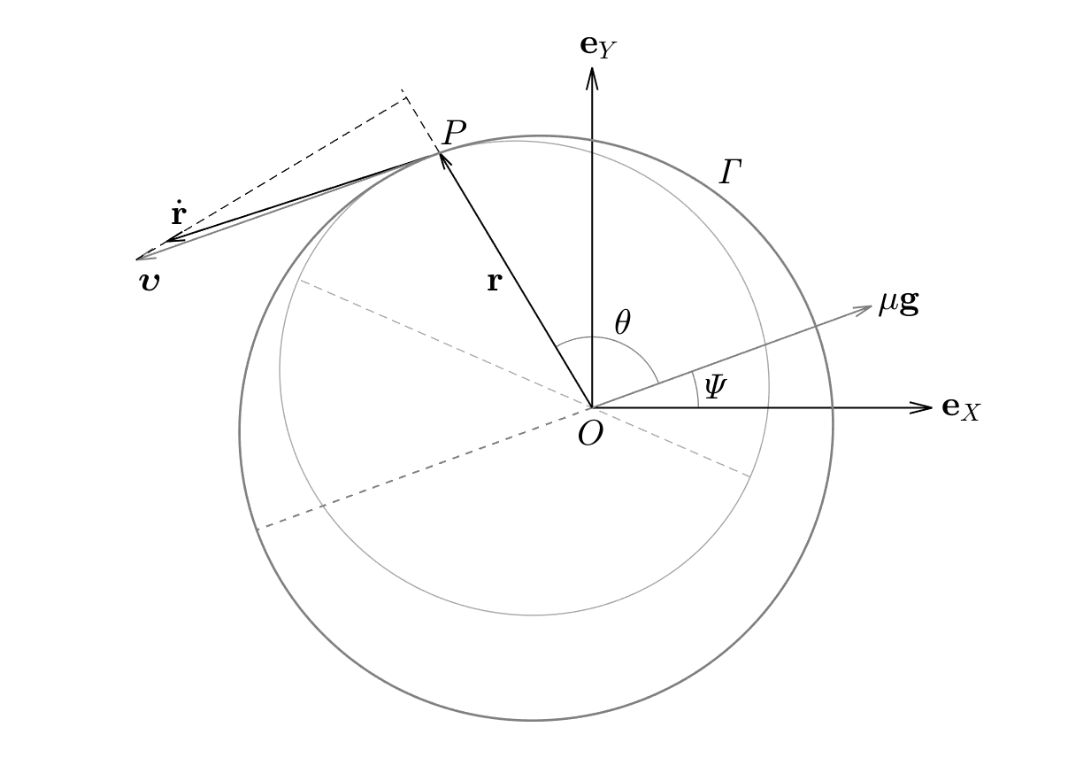
Figure 1: View from the angular momentum vector of the osculating ellipse (in light grey) and the non-osculating ellipse $\Gamma$ described in Section (2.1). The generalized true anomaly $\theta$ and generalized longitude of pericenter $\Psi$ are also shown. The velocities $\dot{\bf r}$ and $\bm{\upsilon}$ of $P$ along the two ellipses have the same radial component $\dot{r}$.

2.2 The elements $\nu$, $p_{1}$, $p_{2}$, $\mathcal{L}$

Consider the classical equinoctial reference frame

$$\Sigma_{\textsf{eq}}=\{O;{\bf e}_{X},{\bf e}_{Y},{\bf e}_{Z}\}.$$

The axis $OX$, associated to ${\bf e}_{X}$, is rotated of $\Omega$ from the ascending node in the retrograde direction; the axis $OY$, associated to ${\bf e}_{Y}$, is rotated of $\pi/2$ from the axis $OX$ in the direction of the motion. The unit vector ${\bf e}_{Z}$ completes the right-handed orthonormal basis. The angular displacement between the direction of ${\bf e}_{r}$ and the departure direction defined by ${\bf e}_{X}$ is called true longitude, and is given by

$$L=\varpi+f,$$ (10)

where

$$\varpi=\omega+\Omega,$$

with $\omega$ the argument of pericenter and $\Omega$ the longitude of the ascending node. We define the angular variable $\Psi$ as

$$\Psi=L-\theta.$$ (11)

When $\mathscr{U}=0$ the angle $\theta$ coincides with $f$ and thereby $\Psi=\varpi$, which becomes constant if we have also ${\bf P}={\bf 0}$. It is straightforward to check that through the angle $\Psi$ we can obtain the direction of the Laplace vector from the direction of ${\bf e}_{X}$, and for this reason we call it the generalized longitude of pericenter (see Figure 1).

The first three elements of the new set are defined as

$$\nu :=\frac{1}{\mu}(-2\mathscr{E})^{3/2},$$ (12)

$$p_{1} :=g\sin\Psi,$$ (13)

$$p_{2} :=g\cos\Psi,$$ (14)

where $\nu$ is the generalized form of the mean motion $n$, and $p_{1}$, $p_{2}$ are the generalized versions of the equinoctial orbital elements $h$, $k$ (Broucke and Cefola, 1972). For later use, we introduce the generalized semi-latus rectum

$$\varrho=\textsl{{a}}(1-g^{2}),$$ (15)

and note that the following formula holds:

$$c^{2}=\mu\varrho,$$ (16)

which is obtained from (6), (7), (15). Moreover, since

a $$=\biggl{(}\frac{\mu}{\nu^{2}}\biggr{)}^{1/3},$$ (17)

$$g^{2} =p_{1}^{2}+p_{2}^{2},$$

we can write $c$ as function of $\nu$, $p_{1}$, $p_{2}$:

$$c=\biggl{(}\frac{\mu^{2}}{\nu}\biggr{)}^{1/3}\sqrt{1-p_{1}^{2}-p_{2}^{2}}.$$ (18)

At this point we need to make another step to define the fourth generalized equinoctial element. We first introduce the generalized eccentric anomaly $G$ through the relations

$$r =\textsl{{a}}(1-g\cos G),$$ (19)

$$r\dot{r} =g\sqrt{\mu\textsl{{a}}}\sin G,$$ (20)

which are analogous to the well-known relations for the Kepler problem

$$r =a(1-e\cos E),$$

$$r\dot{r} =e\sqrt{\mu a}\sin E,$$

where $a$, $E$ are the semi-major axis and eccentric anomaly, respectively. Then, the generalized Kepler’s equation can be written as

$$\mathcal{M}=G-g\sin G,$$ (21)

where $\mathcal{M}$ is the generalized mean anomaly

$$\mathcal{M}=\nu(t-t_{0}),$$ (22)

and $t_{0}$ is the time of passage through the pericenter of the ellipse $\Gamma$ (see Remark 1).

We include in the GEqOE the generalized mean longitude

$$\mathcal{L}:=\mathcal{M}+\Psi.$$ (23)

After defining in a similar way the generalized eccentric longitude as

$$\mathcal{K}=G+\Psi,$$ (24)

we can put equation (22) in the form

$$\mathcal{L}=\mathcal{K}+p_{1}\cos\mathcal{K}-p_{2}\sin\mathcal{K},$$ (25)

where the right-hand side is derived from (21) by taking into account (13), (14), (23), (24). If we know the values of $p_{1}$, $p_{2}$, $\mathcal{L}$ we can compute $\mathcal{K}$ by solving Kepler’s equation (25). The orbital distance and the radial velocity are obtained by means of the formulae:

$$r =\textsl{{a}}(1-p_{1}\sin\mathcal{K}-p_{2}\cos\mathcal{K}),$$ (26)

$$\dot{r} =\frac{\sqrt{\mu\textsl{{a}}}}{r}(p_{2}\sin\mathcal{K}-p_{1}\cos\mathcal{K}),$$ (27)

which follow from equations (19), (20) where we use the definitions (13), (14), (24). Considering also relation (17), we recognize that $r$ and $\dot{r}$ are known from the first four GEqOE, i.e., $\nu$, $p_{1}$, $p_{2}$, $\mathcal{L}$, which are defined in equations (12), (13), (14), (23).

It is worth noting that $r$ and $\dot{r}$ can also be expressed as functions of the true longitude. From equations (8), (9) and (11), (13), (14) we have

$$r =\frac{\varrho}{1+p_{1}\sin L+p_{2}\cos L},$$ (28)

$$\dot{r} =\frac{\mu}{c}(p_{2}\sin L-p_{1}\cos L),$$ (29)

where $\varrho$ is introduced in (15).

2.3 The remaining elements

The three elements $\nu$, $p_{1}$, $p_{2}$ determine the shape and orientation of the non-osculating ellipse $\Gamma$ on the orbital plane, and $\mathcal{L}$ fixes the position of $P$ with respect to $\Sigma_{\textsf{eq}}$. Therefore, the remaining elements of the proposed set need to characterize the orientation of $\Sigma_{\textsf{eq}}$ with respect to $\Sigma$ (see equation 2), which can be recovered by applying the sequence of rotations $\Omega$, $i$, $-\Omega$, where $i$ is the orbital inclination.

The two elements $p$, $q$ in Broucke and Cefola (1972), that is:

$$q_{1} :=\tan\frac{i}{2}\sin\Omega,$$ (30)

$$q_{2} :=\tan\frac{i}{2}\cos\Omega$$ (31)

satisfy our request, and therefore it is natural to include them in the set of GEqOE. An alternative to $q_{1}$, $q_{2}$ is represented by the Euler parameters $e_{1}$, $e_{2}$, $e_{3}$ that define the orientation of $\Sigma_{\textsf{eq}}$ with respect to $\Sigma$ (Goldstein, 1980, p. 155):

$$e_{1}:=\cos\frac{i}{2}\cos\Omega,\quad e_{2}:=\sin\frac{i}{2},\quad e_{3}:=\cos\frac{i}{2}\sin\Omega.$$ (32)

Note that both these elements and $q_{1}$, $q_{2}$ suffer of the singularity for $i=\pi$. The Euler parameters allow us to partially control the error accumulation during the propagation by monitoring the quantity $e_{1}^{2}+e_{2}^{2}+e_{3}^{2}$. On the other hand, they make the set of GEqOE redundant, increasing the dimension of the state vector from 6 to 7. We refer to Section 5.2 for more details about the alternative formulation with $e_{1}$, $e_{2}$, $e_{3}$ in place of $q_{1}$, $q_{2}$.

2.4 Summary

A set of generalized equinoctial orbital elements consists of

$$\nu\,\,({\rm eq.}~{}\ref{eq:enne}),\quad p_{1}\,\,({\rm eq.}~{}\ref{eq:p1}),\quad p_{2}\,\,({\rm eq.}~{}\ref{eq:p2}),\quad\mathcal{L}\,\,({\rm eq.}~{}\ref{eq:elle}),$$

along with

$$q_{1}\,\,({\rm eq.}~{}\ref{eq:q1}),\quad q_{2}\,\,({\rm eq.}~{}\ref{eq:q2}).$$

The generalized mean longitude $\mathcal{L}$ can be replaced by the generalized mean longitude at epoch $\mathcal{L}_{0}$ as shown in Section 5.1. These sets of elements represent two generalizations of the alternate equinoctial orbital elements proposed by Horwood et al (2011) (see the Introduction), with an improved propagation performance, as it will be shown in Section 7.

3 From position and velocity to the GEqOE

Assume that we know the position (${\bf r}$) and velocity ($\dot{\bf r}$) at some time $t$ with respect to the reference frame $\Sigma$ (see equation 2). We want to determine the values of the new elements.

First, we get the quantities

$$r=|{\bf r}|,\qquad\dot{r}=\frac{{\bf r}\cdot\dot{\bf r}}{r},$$

and compute the total energy:

$$\mathscr{E}({\bf r},\dot{\bf r},t)=\mathscr{E}_{K}({\bf r},\dot{\bf r})+\mathscr{U}({\bf r},t),$$

where $\mathscr{E}_{K}$ is the Keplerian energy and the disturbing potential energy $\mathscr{U}$ does not depend on $\dot{\bf r}$. The element $\nu$ is obtained from equation (12).

From the Keplerian orbital elements $\Omega$, $i$, which are determined by classical formulae, we compute $q_{1}$, $q_{2}$ through equations (30), (31), and the unit vectors ${\bf e}_{X}$, ${\bf e}_{Y}$ of the equinoctial reference frame $\Sigma_{\textsf{eq}}$ by

$$\begin{split}{\bf e}_{X}&=\frac{1}{1+q_{1}^{2}+q_{2}^{2}}\left(1-q_{1}^{2}+q_{2}^{2},\,\,2q_{1}q_{2},\,\,-2q_{1}\right)^{T},\\[4.30554pt] {\bf e}_{Y}&=\frac{1}{1+q_{1}^{2}+q_{2}^{2}}\left(2q_{1}q_{2},\,\,1+q_{1}^{2}-q_{2}^{2},\,\,2q_{2}\right)^{T}.\end{split}$$ (33)

Inversion of relations (28), (29) yields

$$p_{1} =\Bigl{(}\frac{\varrho}{r}-1\Bigr{)}\sin L-\frac{c\dot{r}}{\mu}\cos L,$$ (34)

$$p_{2} =\Bigl{(}\frac{\varrho}{r}-1\Bigr{)}\cos L+\frac{c\dot{r}}{\mu}\sin L,$$ (35)

where

$$\cos L={{\bf e}_{r}}\cdot{{\bf e}_{X}},\qquad\sin L={{\bf e}_{r}}\cdot{{\bf e}_{Y}},$$

with ${\bf e}_{r}$ the radial unit vector, and ${\bf e}_{X}$, ${\bf e}_{Y}$ given by (33). The quantity $c$ is obtained using formula (4), wherein $h=|{\bf r}\times\dot{\bf r}|$.

In order to determine the generalized mean longitude $\mathcal{L}$, we need to know the value of the generalized eccentric longitude $\mathcal{K}$. Let us introduce

$$S =(\mu+c\textsl{{w}}-r\dot{r}^{2})\sin L-\dot{r}(c+\textsl{{w}}r)\cos L,$$

$$C =(\mu+c\textsl{{w}}-r\dot{r}^{2})\cos L+\dot{r}(c+\textsl{{w}}r)\sin L.$$

It is possible to show that (see Appendix A)

$$\sin\mathcal{K}=\frac{S}{\mu+c\textsl{{w}}},\quad\cos\mathcal{K}=\frac{C}{\mu+c\textsl{{w}}},$$ (36)

where

$$\textsl{{w}}=\sqrt{\frac{\mu}{\textsl{{a}}}},$$ (37)

and a depends on $\nu$ (see 17). The value of $\mathcal{L}$ is found by means of the generalized Kepler’s equation (25), which is written as

$$\mathcal{L}=\operatorname{atan2}(S,C)+\frac{Cp_{1}-Sp_{2}}{\mu+c\textsl{{w}}}.$$

Finally, we point out that an alternative way to get $p_{1}$, $p_{2}$ is given by the formulae:

$$p_{1} =\frac{1}{\mu+c\textsl{{w}}}\left[\Bigl{(}1-\frac{r}{\textsl{{a}}}\Bigr{)}S-\frac{r\dot{r}}{\sqrt{\mu\textsl{{a}}}}C\right],$$

$$p_{2} =\frac{1}{\mu+c\textsl{{w}}}\left[\frac{r\dot{r}}{\sqrt{\mu\textsl{{a}}}}S+\Bigl{(}1-\frac{r}{\textsl{{a}}}\Bigr{)}C\right],$$

which are derived by solving equations (26), (27) for $p_{1}$, $p_{2}$ and making the substitutions in (36).

4 From the GEqOE to position and velocity

Assume that we know the values taken by the new elements at some time $t$ and we want to find ${\bf r}$ and $\dot{\bf r}$ at that epoch.

We first solve Kepler’s equation (25) for $\mathcal{K}$. Then, we compute a from (17), and obtain $r$ and $\dot{r}$ from (26) and (27). By combining these two equations with (28), (29), and considering (15), (16), we find

$$\begin{split}\sin L&=\frac{\textsl{{a}}}{r}\left[\alpha p_{1}p_{2}\cos\mathcal{K}+(1-\alpha p_{2}^{2})\sin\mathcal{K}-p_{1}\right],\\[4.30554pt] \cos L&=\frac{\textsl{{a}}}{r}\left[\alpha p_{1}p_{2}\sin\mathcal{K}+(1-\alpha p_{1}^{2})\cos\mathcal{K}-p_{2}\right],\end{split}$$ (38)

where

$$\alpha=\frac{1}{1+\sqrt{1-p_{1}^{2}-p_{2}^{2}}}.$$ (39)

After computing the unit vectors ${\bf e}_{X}$, ${\bf e}_{Y}$ of the equinoctial reference frame by means of (33), we can obtain the unit vectors ${\bf e}_{r}$, ${\bf e}_{f}$ of the orbital basis through the rotation:

$$\begin{split}{\bf e}_{r}&={\bf e}_{X}\cos L+{\bf e}_{Y}\sin L,\\[4.30554pt] {\bf e}_{f}&={\bf e}_{Y}\cos L-{\bf e}_{X}\sin L.\end{split}$$ (40)

Finally, the position and velocity vectors are given by the formulae

$${\bf r}=r{\bf e}_{r},\qquad\dot{\bf r}=\dot{r}{\bf e}_{r}+\frac{h}{r}{\bf e}_{f}.$$ (41)

Since the function $\mathscr{U}$ does not depend of $\dot{\bf r}$ we can use equation (4) to calculate $h$:

$$h=\sqrt{c^{2}-2r^{2}\mathscr{U}({\bf r},t)},$$

where $c^{2}$ is obtained from (18).

5 Time derivatives of the GEqOE

The time derivative of $\nu$ is

$$\dot{\nu}=-3\biggl{(}\frac{\nu}{\mu^{2}}\biggr{)}^{\!1/3}\dot{\mathscr{E}},$$ (42)

where

$$\dot{\mathscr{E}}=\mathscr{U}_{t}+{\bf P}\cdot\dot{\bf r}=\mathscr{U}_{t}+\dot{r}P_{r}+\frac{h}{r}P_{f},$$ (43)

and $\mathscr{U}_{t}$ denotes the partial derivative of $\mathscr{U}({\bf r},t)$ with respect to $t$.

The angular velocity of $\Sigma_{\textsf{eq}}$ with respect to $\Sigma$ is

$${\bf w}=w_{X}{\bf e}_{X}+w_{Y}{\bf e}_{Y}+w_{h}{\bf e}_{h},$$

where

$$w_{X} =F_{h}\frac{r}{h}\cos L,$$

$$w_{Y} =F_{h}\frac{r}{h}\sin L,$$

$$w_{h} =\frac{h}{r^{2}}-\dot{L}=-F_{h}\frac{r}{h}\tan{\frac{i}{2}}\sin(\omega+f),$$

and $F_{h}$ is the projection of the perturbing force along ${\bf e}_{h}$. Note that $w_{h}$ is not defined when $i=\pi$. If we divide $w_{X}$, $w_{Y}$, $w_{h}$ by $F_{h}r/h$, and denote the resulting quantities with $\hat{w}_{X}$, $\hat{w}_{Y}$, $\hat{w}_{h}$, we have

$$\begin{split}\hat{w}_{X}&=\cos L,\\ \hat{w}_{Y}&=\sin L,\\ \hat{w}_{h}&=q_{1}\cos L-q_{2}\sin L,\end{split}$$ (44)

where $q_{1}$, $q_{2}$ are defined in (30), (31). The expression for $\hat{w}_{h}$ is obtained noting that

$$\omega+f=L-\Omega.$$

For the time derivatives of $p_{1}$, $p_{2}$ we find (see the derivation in Appendix B)

$$\dot{p}_{1} =p_{2}\biggl{(}\frac{h-c}{r^{2}}-\frac{r}{h}\hat{w}_{h}F_{h}\biggr{)}+\frac{1}{c}\Bigl{(}\frac{r\dot{r}}{c}p_{1}+\tilde{\varsigma}p_{2}+\varsigma\cos L\Bigr{)}(2\mathscr{U}-rF_{r})$$

$$\quad\,+\frac{r}{\mu}(\varsigma\,p_{1}+\tilde{\varsigma}\sin L)\dot{\mathscr{E}},$$ (45)

$$\dot{p}_{2} =p_{1}\biggl{(}\frac{r}{h}\hat{w}_{h}F_{h}-\frac{h-c}{r^{2}}\biggr{)}+\frac{1}{c}\Bigl{(}\frac{r\dot{r}}{c}p_{2}-\tilde{\varsigma}p_{1}-\varsigma\sin L\Bigr{)}(2\mathscr{U}-rF_{r})$$

$$\quad\,+\frac{r}{\mu}(\varsigma\,p_{2}+\tilde{\varsigma}\cos L)\dot{\mathscr{E}},$$ (46)

where $F_{r}={\bf F}\cdot{\bf e}_{r}$, $F_{h}={\bf F}\cdot{\bf e}_{h}$ and we use the non-dimensional quantities

$$\varsigma=\frac{r}{\varrho},\qquad\tilde{\varsigma}=1+\varsigma.$$ (47)

Concerning the element $\mathcal{L}$, we can write (see the derivation in Appendix C)

$$\begin{split}\dot{\mathcal{L}}&=\nu+\frac{h-c}{r^{2}}-\frac{r}{h}\hat{w}_{h}F_{h}+\Bigl{(}\frac{r\dot{r}c}{\mu^{2}}\tilde{\varsigma}\alpha\Bigr{)}\dot{\mathscr{E}}\\ &\quad\,+\frac{1}{c}\biggl{[}\frac{1}{\alpha}+\alpha\Bigl{(}1-\frac{r}{\textsl{{a}}}\Bigr{)}\biggr{]}(2\mathscr{U}-rF_{r}),\end{split}$$ (48)

where $\alpha$ is defined in (39). For the remaining two elements $q_{1}$, $q_{2}$ we need the derivatives (see Battin, 1999, eqs. 10.51, 10.52, p. 493)

$$\dot{q}_{1} =\frac{r}{2h}F_{h}(1+q_{1}^{2}+q_{2}^{2})\sin L,$$ (49)

$$\dot{q}_{2} =\frac{r}{2h}F_{h}(1+q_{1}^{2}+q_{2}^{2})\cos L.$$ (50)

The right-hand side of equations (42), (45), (46), (C), (49), (50) can be efficiently computed by following the procedure outlined in Section 4.

5.1 Constant time element

The equinoctial elements presented in Broucke and Cefola (1972) comprise the mean longitude at epoch $\lambda_{0}=\varpi+nt_{0}$, where we recall that $n$ is the mean motion and $t_{0}$ the time of pericenter passage. This quantity is a constant of the motion when the perturbations are turned off, and being related to the physical time we can refer to $\lambda_{0}$ as a constant time element. On the other hand, the generalized mean longitude $\mathcal{L}$ included in the GEqOE varies linearly with time along Keplerian motion (see equation C), and therefore it is a linear time element.

In place of $\mathcal{L}$, we may consider the generalized mean motion at epoch $\mathcal{L}_{0}$, which we define as

$$\mathcal{L}_{0}:=\Psi-\nu t_{0}.$$

Using equations (22), (23), we see that

$$\mathcal{L}_{0}=\mathcal{L}-\nu t,$$

and therefore its time derivative can be computed from (42), (C), resulting in

$$\dot{\mathcal{L}}_{0} =\frac{h-c}{r^{2}}-\frac{r}{h}\hat{w}_{h}F_{h}+\biggl{[}3t\biggl{(}\frac{\nu}{\mu}\biggr{)}^{\!1/3}+\frac{r\dot{r}c}{\mu^{2}}\tilde{\varsigma}\alpha\biggr{]}\dot{\mathscr{E}}$$

$$\quad\,+\frac{1}{c}\biggl{[}\frac{1}{\alpha}+\alpha\Bigl{(}1-\frac{r}{\textsl{{a}}}\Bigr{)}\biggr{]}(2\mathscr{U}-rF_{r}),$$

where $\alpha$, $\tilde{\varsigma}$ are introduced in (39), (68). We note that a term dependent explicitly on time arises in the expression of $\dot{\mathcal{L}}_{0}$, which is not present in $\dot{\mathcal{L}}$. For long-term propagations this term may grow enough to deteriorate the efficiency of the propagation.

5.2 Alternative formulation

If the Euler parameters $e_{1}$, $e_{2}$, $e_{3}$ given in (32) are used in place of $q_{1}$, $q_{2}$, then, ${\bf e}_{X}$, ${\bf e}_{Y}$ are computed from the formulae

$${\bf e}_{X} =\left(e_{1}^{2}+e_{2}^{2}-e_{3}^{2},\,\,-2e_{1}e_{3},\,\,2e_{2}e_{3}\right)^{T},$$

$${\bf e}_{Y} =\left(2e_{1}e_{3},\,\,e_{1}^{2}-e_{2}^{2}-e_{3}^{2},\,\,-2e_{1}e_{2}\right)^{T}.$$

The time derivatives of the Euler parameters read

$$\dot{e}_{1} =\frac{r}{2h}F_{h}(\hat{w}_{h}e_{2}+\hat{w}_{X}e_{3}),$$

$$\dot{e}_{2} =-\frac{r}{2h}F_{h}(\hat{w}_{h}e_{1}-\hat{w}_{Y}e_{3}),$$

$$\dot{e}_{3} =-\frac{r}{2h}F_{h}(\hat{w}_{X}e_{1}+\hat{w}_{Y}e_{2}),$$

where $\hat{w}_{X}$, $\hat{w}_{Y}$ are defined in (44) and

$$\hat{w}_{h}=\frac{e_{2}}{e_{1}^{2}+e_{3}^{2}}(e_{3}\cos L-e_{1}\sin L),$$

with $\sin L$, $\cos L$ obtained by (38).

6 The fundamental matrix and its inverse

The fundamental matrix is defined as the matrix of the partial derivatives of position and velocity with respect to the set of elements used for describing the motion (Broucke, 1970). We consider in this section the two sets of GEqOE given by $\nu$, $p_{1}$, $p_{2}$, $q_{1}$, $q_{2}$, along with either $\mathcal{L}$ or $\mathcal{L}_{0}$. In Broucke and Cefola (1972), the fundamental matrix and its inverse are expressed using the perifocal reference frame. However, since its basis is not defined when the eccentricity is zero, we prefer to have the unit vectors of the equinoctial and orbital reference frames appearing directly in (52), (53), (54), (55) (see Danielson et al, 1995). We use the notation:

$$X =r\cos L, Y =r\sin L,$$

$$\dot{X} =\dot{r}\cos L-\frac{h}{r}\sin L, \dot{Y} =\dot{r}\sin L+\frac{h}{r}\cos L,$$

for the components of the position and velocity vectors along the directions of the unit vectors ${\bf e}_{X}$, ${\bf e}_{Y}$, that is

$${\bf r}=X{\bf e}_{X}+Y{\bf e}_{Y},\qquad\dot{\bf r}=\dot{X}{\bf e}_{X}+\dot{Y}{\bf e}_{Y}.$$

Moreover, we introduce the non-dimensional quantities

$$\beta =\sqrt{1-p_{1}^{2}-p_{2}^{2}}, \gamma =1+q_{1}^{2}+q_{2}^{2},$$ (51)

where $\beta=0$, $\gamma=0$ when $g=0$, $i=\pi$, respectively.

6.1 Partial derivatives of position and velocity with respect to the GEqOE

We obtain the partial derivatives of ${\bf r}$, $\dot{\bf r}$ with respect to the GEqOE by direct differentiation of equations (41), wherein $r$, $\dot{r}$ and ${\bf e}_{r}$, ${\bf e}_{f}$ are replaced by the expressions reported in (26), (27) and (40), respectively. Relations (25), (38) are also necessary. Regarding the position, we have:

$$\begin{split}\frac{\partial{\bf r}}{\partial\nu}&=-\frac{2}{3\nu}{\bf r},\\[4.30554pt] \frac{\partial{\bf r}}{\partial p_{1}}&=-\textsl{{a}}\Bigl{(}\frac{\alpha p_{2}}{\beta}{\bf q}+{\bf e}_{Y}\Bigr{)}-\frac{\textsl{{a}}}{\varrho}\left[X+p_{2}(r+\alpha\beta\textsl{{a}})\right]{\bf e}_{f},\\[4.30554pt] \frac{\partial{\bf r}}{\partial p_{2}}&=\textsl{{a}}\Bigl{(}\frac{\alpha p_{1}}{\beta}{\bf q}-{\bf e}_{X}\Bigr{)}+\frac{\textsl{{a}}}{\varrho}\left[Y+p_{1}(r+\alpha\beta\textsl{{a}})\right]{\bf e}_{f},\\[4.30554pt] \frac{\partial{\bf r}}{\partial\mathcal{L}}&=\frac{1}{\nu}{\bm{\upsilon}},\\[4.30554pt] \frac{\partial{\bf r}}{\partial q_{1}}&=-\frac{2}{\gamma}(rq_{2}{\bf e}_{f}+X{\bf e}_{h}),\\[4.30554pt] \frac{\partial{\bf r}}{\partial q_{2}}&=\frac{2}{\gamma}(rq_{1}{\bf e}_{f}+Y{\bf e}_{h}),\end{split}$$ (52)

where the generalized velocity $\bm{\upsilon}$ and the non-dimensional quantity $\alpha$ are introduced in (5), (39), respectively, and

$${\bf q}=p_{2}{\bf e}_{Y}-p_{1}{\bf e}_{X}.$$

Remark 2. It is possible to prove that the derivatives of ${\bf r}$ with respect to a, $p_{1}$, $p_{2}$, $\tilde{\mathcal{L}}_{0}$ (see the footnote 5), $q_{1}$, $q_{2}$ can be written in the same form as the derivatives of ${\bf r}$ with respect to $a$, $h$, $k$, $\lambda_{0}$, $p$, $q$ that are reported in Broucke and Cefola (1972, Table I). We just have to replace in the latters the osculating eccentric anomaly ($E$), eccentricity ($e$), semi-major axis ($a$), longitude of pericenter ($\omega+\Omega$) by $G$, $g$, a, $\Psi$, respectively, and the unit vectors ${\bf e}_{p}$, ${\bf e}_{q}$ of the perifocal reference frame by their generalized versions ${\bf e}_{p}^{\prime}$, ${\bf e}_{q}^{\prime}$, which are defined as (see also Figure 2)

$${\bf e}_{p}^{\prime} ={\bf e}_{X}\cos\Psi+{\bf e}_{Y}\sin\Psi,$$

$${\bf e}_{q}^{\prime} ={\bf e}_{Y}\cos\Psi-{\bf e}_{X}\sin\Psi,$$

where $\Psi$ is given in (11).

The partial derivatives of the velocity with respect to the GEqOE are:

$$\begin{split}\frac{\partial{\dot{\bf r}}}{\partial\nu}&=\frac{1}{3\nu}\dot{\bf r}+f_{0}{\bf e}_{f},\\[4.30554pt] \frac{\partial{\dot{\bf r}}}{\partial p_{1}}&=-\frac{\mu\textsl{{a}}}{r}\biggl{[}\frac{2\sigma_{1}}{\mu\beta}{\dot{\bf r}}+\Bigl{(}\frac{p_{2}}{r\textsl{{w}}}-\frac{\sigma_{2}}{c}\Bigr{)}{\bf e}_{r}+\frac{p_{1}}{h}{\bf e}_{f}\biggr{]}+\frac{1}{r}{\bf s}_{1}+f_{1}{\bf e}_{f},\\[4.30554pt] \frac{\partial{\dot{\bf r}}}{\partial p_{2}}&=-\frac{\mu\textsl{{a}}}{r}\biggl{[}\frac{2\sigma_{2}}{\mu\beta}{\dot{\bf r}}-\Bigl{(}\frac{p_{1}}{r\textsl{{w}}}-\frac{\sigma_{1}}{c}\Bigr{)}{\bf e}_{r}+\frac{p_{2}}{h}{\bf e}_{f}\biggr{]}+\frac{1}{r}{\bf s}_{2}+f_{2}{\bf e}_{f},\\[4.30554pt] \frac{\partial{\dot{\bf r}}}{\partial\mathcal{L}}&=\frac{1}{r\nu}\biggl{[}-2\dot{r}\dot{\bf r}+\frac{\mu}{r}\Bigl{(}1-\frac{r}{\textsl{{a}}}\Bigr{)}{\bf e}_{r}\biggr{]}+\frac{1}{r}{\bf s}_{3}+f_{3}{\bf e}_{f},\\[4.30554pt] \frac{\partial{\dot{\bf r}}}{\partial q_{1}}&=\frac{2}{\gamma}(q_{2}\dot{\bf r}\times{\bf e}_{h}-\dot{X}{\bf e}_{h})+f_{4}{\bf e}_{f},\\[4.30554pt] \frac{\partial{\dot{\bf r}}}{\partial q_{2}}&=-\frac{2}{\gamma}(q_{1}\dot{\bf r}\times{\bf e}_{h}-\dot{Y}{\bf e}_{h})+f_{5}{\bf e}_{f},\end{split}$$ (53)

where the variable w is defined in (37),

$$f_{0} =\frac{r}{h}\biggl{(}\frac{2}{3\nu}\mathscr{U}-\frac{\partial{\mathscr{U}}}{\partial\nu}\biggr{)},$$

$$f_{i} =-\frac{1}{h}\biggl{(}\frac{2\sigma_{i}\textsl{{a}}}{\beta}\mathscr{U}+r\frac{\partial\mathscr{U}}{\partial p_{i}}\biggr{)},\quad i=1,2,$$

$$f_{3} =-\frac{1}{h}\biggl{(}\frac{2\dot{r}}{\nu}\mathscr{U}+r\frac{\partial\mathscr{U}}{\partial\mathcal{L}}\biggr{)},$$

$$f_{i+3} =-\frac{r}{h}\frac{\partial\mathscr{U}}{\partial q_{i}},\quad i=1,2,$$

and

$$\sigma_{1} =\frac{1}{r}[\alpha p_{1}(\varrho-r)-Y],$$

$$\sigma_{2} =\frac{1}{r}[\alpha p_{2}(\varrho-r)-X],$$

$${\bf s}_{i} =\dot{r}\frac{\partial{\bf r}}{\partial p_{i}}+\frac{h}{r}{\bf e}_{h}\times\frac{\partial{\bf r}}{\partial p_{i}},\qquad i=1,2,$$

$${\bf s}_{3} =\dot{r}\frac{\partial{\bf r}}{\partial\mathcal{L}}+\frac{h}{r}{\bf e}_{h}\times\frac{\partial{\bf r}}{\partial\mathcal{L}}.$$

In (53) the terms $f_{i},\,(i=1,\dots,5)$ are equal to zero if $\mathscr{U}=0$.

If the constant time element $\mathcal{L}_{0}$ is used instead of $\mathcal{L}$, we have

$$\frac{\partial{\bf r}}{\partial\nu} =\frac{1}{\nu}\Bigl{(}t{\bm{\upsilon}}-\frac{2}{3}{\bf r}\Bigr{)},$$

$$\frac{\partial{\bf r}}{\partial\mathcal{L}_{0}} =\frac{\partial{\bf r}}{\partial\mathcal{L}},$$

and

$$\frac{\partial{\dot{\bf r}}}{\partial\nu} =\frac{1}{3\nu}\dot{\bf r}+f_{0}{\bf e}_{f}+\frac{t}{r^{2}\nu}\left(\frac{c}{h}(c-h)\,\dot{\bf r}\times{\bf e}_{h}-\mu{\bf e}_{r}\right),$$

$$\frac{\partial{\dot{\bf r}}}{\partial\mathcal{L}_{0}} =\frac{\partial{\dot{\bf r}}}{\partial\mathcal{L}}.$$

On the other hand, the partial derivatives of ${\bf r}$, $\dot{\bf r}$ with respect to $p_{1}$, $p_{2}$, $q_{1}$, $q_{2}$ remain the same as in (52), (53).

Remark 3. The partial derivative of $\mathscr{U}$ with respect to any element $\chi$ of our set of GEqOE is computed by the chain rule

$$\frac{\partial{\mathscr{U}}}{\partial\chi}=\frac{\partial{\mathscr{U}}}{\partial{\bf r}}\frac{\partial{\bf r}}{\partial\chi}.$$

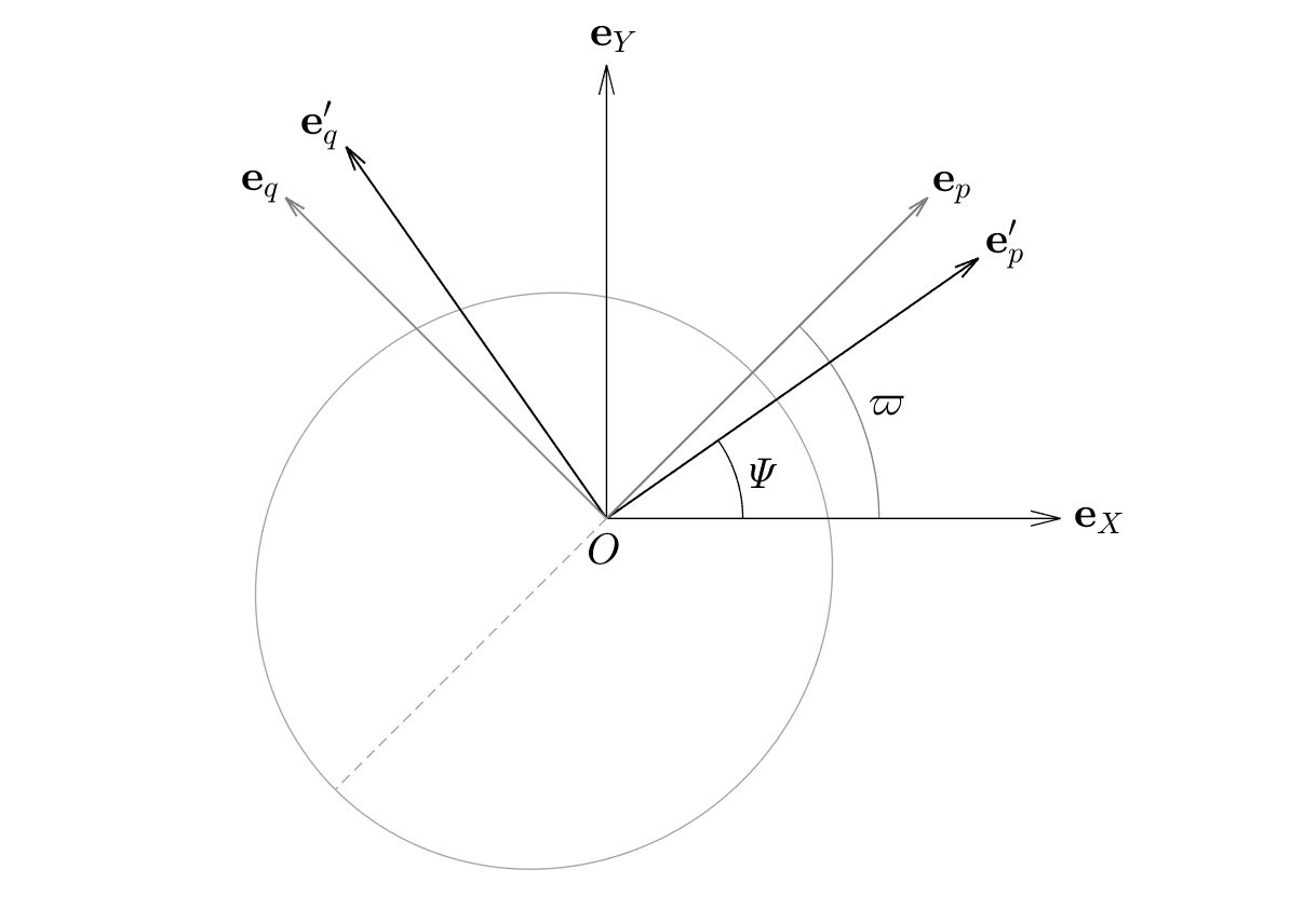
Figure 2: View from the angular momentum vector of the unit vectors ${\bf e}_{X}$, ${\bf e}_{Y}$ of the equinoctial basis, and of ${\bf e}_{p}^{\prime}$, ${\bf e}_{q}^{\prime}$, which are the generalized counterparts of the unit vectors ${\bf e}_{p}$, ${\bf e}_{q}$ of the perifocal basis.

6.2 Partial derivatives of the GEqOE with respect to position and velocity

The inverse of the fundamental matrix for the equinoctial elements is obtained in Broucke and Cefola (1972) using the Poisson brackets and the fundamental matrix (see also Broucke, 1970). Here, we proceed as follows. As concerns the elements $q_{1}$, $q_{2}$, we simply put the expressions given in Broucke and Cefola (1972, Table III) for the derivatives of $p$, $q$ in a suitable form to avoid singularities for small eccentricities and inclinations (as in Danielson et al, 1995). For the generalized mean motion $\nu$ we started from equation (12) and used the definition of the total energy. The computation for the elements $p_{1}$, $p_{2}$ was done considering equations (34), (35) and taking into account (10). Finally, concerning $\mathcal{L}$ and $\mathcal{L}_{0}$, equations (25), (26), (27) were used.

The partial derivatives with respect to the position and velocity read

$$\begin{split}\frac{\partial\nu}{\partial{\bf r}}&=-\frac{3\textsl{{a}}\nu}{r^{2}}{\bf e}_{r}^{T}+{\bf f}_{0},\\[4.30554pt] \frac{\partial p_{1}}{\partial{\bf r}}&=\frac{1}{r}(p_{1}+\sin L){\bf e}_{r}^{T}-\frac{h}{cr}\biggl{[}\Bigl{(}2-\frac{c}{h}\Bigr{)}p_{2}+\frac{X}{\textsl{{a}}}\biggr{]}{\bf e}_{f}^{T}-\frac{p_{2}\Lambda}{h}{\bf e}_{h}^{T}+{\bf f}_{1},\\[4.30554pt] \frac{\partial p_{2}}{\partial{\bf r}}&=\frac{1}{r}(p_{2}+\cos L){\bf e}_{r}^{T}+\frac{h}{cr}\biggl{[}\Bigl{(}2-\frac{c}{h}\Bigr{)}p_{1}+\frac{Y}{\textsl{{a}}}\biggr{]}{\bf e}_{f}^{T}+\frac{p_{1}\Lambda}{h}{\bf e}_{h}^{T}+{\bf f}_{2},\\[4.30554pt] \frac{\partial\mathcal{L}}{\partial{\bf r}}&=\frac{\dot{r}}{cr}(\varrho\alpha-r\beta){\bf e}_{r}^{T}-\frac{h}{cr}\Bigl{(}2-\frac{c}{h}+\frac{\alpha}{\textsl{{a}}}(\varrho-r)\Bigr{)}{\bf e}_{f}^{T}-\frac{\Lambda}{h}{\bf e}_{h}^{T}+{\bf f}_{3},\\[4.30554pt] \frac{\partial q_{1}}{\partial{\bf r}}&=-\frac{\gamma\dot{Y}}{2h}{\bf e}_{h}^{T},\\[4.30554pt] \frac{\partial q_{2}}{\partial{\bf r}}&=-\frac{\gamma\dot{X}}{2h}{\bf e}_{h}^{T},\end{split}$$ (54)

and

$$\begin{split}\frac{\partial\nu}{\partial{\dot{\bf r}}}&=-\frac{3}{\sqrt{\mu\textsl{{a}}}}\dot{\bf r}^{T},\\[4.30554pt] \frac{\partial p_{1}}{\partial{\dot{\bf r}}}&=-\frac{c}{\mu}\cos L\,{\bf e}_{r}^{T}+\frac{h}{\mu}\Bigl{(}2\sin L-\frac{\dot{r}}{c}X\Bigr{)}{\bf e}_{f}^{T}+\frac{p_{2}\lambda}{h}{\bf e}_{h}^{T},\\[4.30554pt] \frac{\partial p_{2}}{\partial{\dot{\bf r}}}&=\frac{c}{\mu}\sin L\,{\bf e}_{r}^{T}+\frac{h}{\mu}\Bigl{(}2\cos L+\frac{\dot{r}}{c}Y\Bigr{)}{\bf e}_{f}^{T}-\frac{p_{1}\lambda}{h}{\bf e}_{h}^{T},\\[4.30554pt] \frac{\partial\mathcal{L}}{\partial{\dot{\bf r}}}&=\Bigl{(}\frac{c}{\mu r}\alpha(r-\varrho)-\frac{2r}{\sqrt{\mu\textsl{{a}}}}\Bigr{)}{\bf e}_{r}^{T}+\frac{h\dot{r}}{c\mu}\alpha(\varrho+r){\bf e}_{f}^{T}+\frac{\lambda}{h}{\bf e}_{h}^{T},\\[4.30554pt] \frac{\partial q_{1}}{\partial{\dot{\bf r}}}&=\frac{\gamma Y}{2h}{\bf e}_{h}^{T},\\[4.30554pt] \frac{\partial q_{2}}{\partial{\dot{\bf r}}}&=\frac{\gamma X}{2h}{\bf e}_{h}^{T},\end{split}$$ (55)

where

$${\bf f}_{0} =-\frac{3}{\sqrt{\mu\textsl{{a}}}}\frac{\partial{\mathscr{U}}}{\partial{\bf r}},$$

$${\bf f}_{1} =\frac{1}{\mu\varrho}\left[(\varrho+r)Y+p_{1}r^{2}\right]\frac{\partial\mathscr{U}}{\partial{\bf r}},$$

$${\bf f}_{2} =\frac{1}{\mu\varrho}\left[(\varrho+r)X+p_{2}r^{2}\right]\frac{\partial\mathscr{U}}{\partial{\bf r}},$$

$${\bf f}_{3} =\frac{r\dot{r}}{c\mu}(\varrho+r)\alpha\frac{\partial\mathscr{U}}{\partial{\bf r}},$$

and

$$\lambda=Yq_{2}-Xq_{1},\qquad\Lambda=\dot{Y}q_{2}-\dot{X}q_{1}.$$

The vectors ${\bf f}_{i}$ ($i=0,\ldots,3$) are equal to zero if $\mathscr{U}=0$.

Finally, the partial derivatives of the constant time element $\mathcal{L}_{0}$ are given by

$$\frac{\partial\mathcal{L}_{0}}{\partial{\bf r}} =\frac{\partial\mathcal{L}}{\partial{\bf r}}-3t\Bigl{(}\frac{\alpha}{r^{2}}{\bf e}_{r}^{T}-\frac{1}{\sqrt{\mu\textsl{{a}}}}\frac{\partial\mathscr{U}}{\partial{\bf r}}\Bigr{)},$$

$$\frac{\partial\mathcal{L}_{0}}{\partial{\dot{\bf r}}} =\frac{\partial\mathcal{L}}{\partial{\dot{\bf r}}}+\frac{3t}{\sqrt{\mu\textsl{{a}}}}\dot{\bf r}^{T}.$$

Remark 4. If $\mathcal{L}_{0}$ is employed in place of $\mathcal{L}$, terms that are linear in time are introduced in the expressions of $\partial{{\bf r}}/\partial{\nu}$, $\partial{\dot{\bf r}}/\partial{\nu}$, $\partial{\mathcal{L}_{0}}/\partial{{\bf r}}$, $\partial{\mathcal{L}_{0}}/\partial{\dot{\bf r}}$.

7 Numerical tests

We employ the generalized equinoctial elements (GEqOE) $\nu$, $p_{1}$, $p_{2}$, $\mathcal{L}$, $q_{1}$, $q_{2}$ (Section 2.4) to propagate the motion of an artificial satellite around the Earth. Starting from the case in which only the perturbation due to the $J_{2}$ zonal harmonic of the geopotential is considered, we then add the third-body gravitational attraction of the Moon and Sun. The GEqOE are compared to the alternate equinoctial orbital elements (AEqOE) presented in Horwood et al (2011, Section 10.4) and Cowell’s method. We deliberately select a very simple numerical integrator, which is a fourth order Runge-Kutta with a fixed step size, in order to highlight the impact of the particular set of elements on the propagation performance. The errors are computed by taking as true the solution obtained by using the Dromo(PC) formulation presented in Baù and Bombardelli (2014) and an adaptive step size Runge-Kutta Dormand-Prince 5(4)7FM method described in Dormand and Prince (1980) with a tolerance of $10^{-13}$.

7.1 The main problem

Let us introduce an Earth-centered inertial reference frame. In particular, we denote by $Oz$ the axis pointing to the North Pole and by ${\bf e}_{z}$ the corresponding unit vector. We consider here the unrealistic case in which the perturbing force ${\bf F}$ (see equation 3) is given by

$${\bf F}=\nabla\mathscr{R}({\bf r}),$$

where $\mathscr{R}$ is the disturbing potential associated with the $J_{2}$ term of the Earth’s gravitational field:

$$\mathscr{R}=-\mathscr{U}=\frac{A}{r^{3}}(1-3\hat{z}^{2}),$$ (56)

with

$$A=\frac{GMJ_{2}r_{eq}^{2}}{2},\qquad\hat{z}=\frac{z}{r},$$

and $z={\bf r}\cdot{\bf e}_{z}$. The quantity $r_{eq}$ denotes the equatorial radius of the Earth. We have

$${\bf F}=-\frac{3A}{r^{4}}\bigl{[}(1-5\hat{z}^{2}){\bf e}_{r}+2\hat{z}{\bf e}_{z}\bigr{]}.$$

In the differential equations of the generalized equinoctial elements the perturbing force appears only as $2\mathscr{U}-rF_{r}$, $r\hat{w}_{h}F_{h}$, $rF_{h}$, where $F_{r}={\bf F}\cdot{\bf e}_{r}$, $F_{h}={\bf F}\cdot{\bf e}_{h}$. A straightforward computation yields

$$2\mathscr{U}-rF_{r}=-\mathscr{U},$$

$$r\hat{w}_{h}F_{h}=\frac{3A}{r^{3}}\hat{z}^{2}(1-q_{1}^{2}-q_{2}^{2})=\frac{3A}{hr^{3}}\hat{z}^{2}\,\mathscr{C}(1+q_{1}^{2}+q_{2}^{2}),$$

$$rF_{h}=-\frac{6A}{hr^{3}}\hat{z}\,\mathscr{C},$$

where we used the relation

$$\cos i=\frac{\mathscr{C}}{h},$$

and $\mathscr{C}$ is the component of the angular momentum vector along $Oz$, which is a first integral of the motion. Taking into account that the total energy $\mathscr{E}$ is also a first integral in this case, the time derivatives of the GEqOE become

$$\dot{\nu} =0,$$

$$\dot{p}_{1} =p_{2}\biggl{(}\frac{h-c}{r^{2}}-I\hat{z}\biggr{)}-\frac{1}{c}\Bigl{(}\frac{r\dot{r}}{c}p_{1}+\tilde{\varsigma}p_{2}+\varsigma\cos L\Bigr{)}\mathscr{U},$$

$$\dot{p}_{2} =-p_{1}\biggl{(}\frac{h-c}{r^{2}}-I\hat{z}\biggr{)}-\frac{1}{c}\Bigl{(}\frac{r\dot{r}}{c}p_{2}-\tilde{\varsigma}p_{1}-\varsigma\sin L\Bigr{)}\mathscr{U},$$

$$\dot{\mathcal{L}}_{0} =\frac{h-c}{r^{2}}-I\hat{z}-\frac{1}{c}\biggl{[}\frac{1}{\alpha}+\alpha\Bigl{(}1-\frac{r}{\textsl{{a}}}\Bigr{)}\biggr{]}\mathscr{U},$$

$$\dot{q}_{1} =-I\sin L,$$

$$\dot{q}_{2} =-I\cos L,$$

where

$$I=\frac{3A}{h^{2}r^{3}}\hat{z}\,\mathscr{C}(1+q_{1}^{2}+q_{2}^{2}).$$

The meaning of the variables a, $\alpha$, $\tilde{\varsigma}$, $\varsigma$ is explained in (6), (39), (68). In the equations above the quantities $\mathscr{C}$, a, $\nu$ remain constant along the motion and their values are determined by the initial position (${\bf r}$) and velocity ($\dot{\bf r}$). In particular, the value of the element $\nu$ is computed by (see equation 12)

$$\nu=\frac{1}{\mu}\biggl{[}\frac{2A}{r_{*}^{3}}(1-3\hat{z}_{*}^{2})-|{\dot{\bf r}}_{*}|^{2}\biggr{]}^{3/2},$$

where $r_{*}$, $\hat{z}_{*}$, ${\dot{\bf r}}_{*}$ refer to the starting epoch of the propagation.

Table 1: Initial conditions for the numerical tests: $r_{p}$ is the radius of perigee in km, $e$, $i$, $\Omega$, $\omega$, $M_{0}$ are Keplerian elements. Angular variables are given in degrees and expressed with respect the J2000 frame.

	$r_{p}$	$e$	$i$	$\Omega$	$\omega$	$M_{0}$
1)	7178.1366	0	45	0	0	0
2)	7178.1366	0	90	0	0	0
3)	26000	0.74	63.4	30	270	0

The initial conditions specified in the row labeled 1) in Table 1, which correspond to a low Earth orbit, are propagated for 12 days. Figure 3 shows the position error at the final time obtained with different values of the integration step size. The same initial conditions are then propagated for 365 days using a step size of 1 minute. The time evolution of the errors in the position and total energy are displayed in Figure 4. It is evident that the GEqOE are much better than the EqOE and Cowell’s method for this test case.

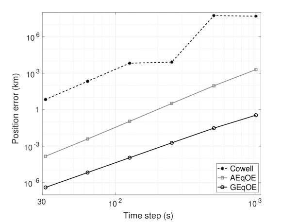
Figure 3: Position error after 12 days of propagation for increasing values of the integration step size. The initial conditions correspond to the low Earth orbit reported in the row 1) of Table 1. Only the perturbation arising from the $J_{2}$ zonal harmonic of the geopotential is considered. Note that a logarithmic scale is applied to both axes.

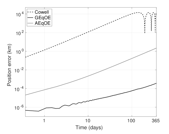
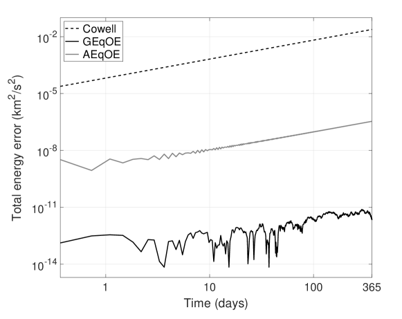
Figure 4: Time evolution of (top) the position error and (bottom) the error of the total energy throughout 365 days of propagation of the initial conditions reported in the row 1) of Table 1. Only the perturbation arising from the $J_{2}$ zonal harmonic of the geopotential is considered. Note that a logarithmic scale is applied to both axes.

7.2 $J_{2}$ and third-body perturbations

Third-body perturbing forces due to the gravitational attraction of the Moon and Sun are switched on in the following tests. Since we decided to not derive them from a potential, these forces determine the vector ${\bf P}$ in equation (3). On the other hand, the force exerted by the Earth’s oblateness is derived from the potential $\mathscr{R}$ introduced in (56).

The same performance plots shown in Section 7.1 are obtained for the initial conditions reported in the rows 2) and 3) of Table 1, which correspond to a low Earth orbit and a Molniya orbit. The initial epoch of the propagations is January 1, 2020 UTC. For a short-term propagation (in the order of a few days), we display in Figure 5 the variation of the position error referred to the final time as the step size of the integrator is enlarged. Then, for a long-term propagation (in the order of hundreds of days) Figure 6 shows the time evolution of the position error using a step size of 1 minute. The timespan of the Molniya orbit propagation was chosen about 7 times larger in order to have the same number of revolutions as the case of the low Earth orbit.

From these results we see that third-body perturbations do not deteriorate the performance of the GEqOE, when compared to the case in which only a conservative perturbation is present. The generalized equinoctial orbital elements brings a substantial improvement with respect to the AEqOE and Cowell’s method.

Because the Molniya orbit is quite eccentric, it is reasonable to use also a variable step size numerical integrator: we chose the same Runge-Kutta Dormand-Prince method that provides the true solution. The relative tolerance controls the selection of the step size and tighter tolerances imply shorter steps. The total number of evaluations of the vector field at the end of the propagation can be taken as a measure of the computational cost. In Figure 7 we show for decreasing values of the relative tolerance the number of evaluations and the corresponding maximum position error reached in a 85.6 days propagation interval. We denote with GEqOE(c) the set of generalized orbital elements in which $\mathcal{L}_{0}$ (see Section 5.1) is employed instead of $\mathcal{L}$. While in the previous numerical tests GEqOE and GEqOE(c) exhibit an almost identical performance, in this test the latter formulation is better: it is faster and decreases the minimum achievable position error. We see that the formulations GEqOE and GEqOE(c) are much more efficient than AEqOE and Cowell’s method.

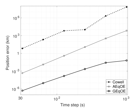
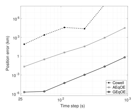
Figure 5: Position error for increasing values of the integration step size. The initial conditions correspond to (top) the low Earth orbit and (bottom) the Molniya orbit reported in the rows 2) and 3), respectively, of Table 1. The former is propagated for 12 days, the latter for 85.6 days. Perturbations due to the $J_{2}$ zonal harmonic of the geopotential and the attraction of the Moon and Sun are considered. Note that a logarithmic scale is applied to both axes.

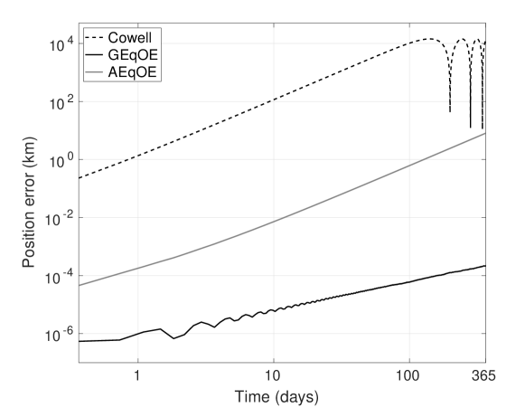
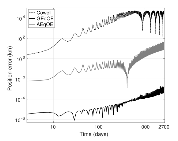
Figure 6: Time evolution of the position error. The initial conditions correspond to (top) the low Earth orbit and (bottom) the Molniya orbit reported in the rows 2) and 3), respectively, of Table 1. The former is propagated for 365 days, the latter for 2604 days. Perturbations due to the $J_{2}$ zonal harmonic of the geopotential and the attraction of the Moon and Sun are considered. Note that a logarithmic scale is applied to both axes.

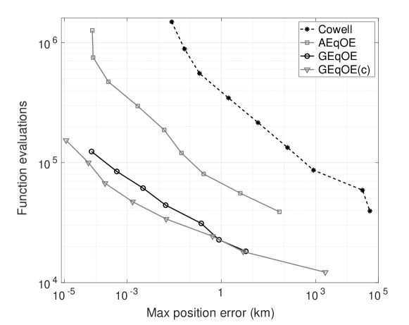
Figure 7: Function evaluations (see the text) versus maximum position error in 85.6 days of propagation for decreasing (right to left) values of the integrator relative tolerance. The initial conditions correspond to the Molniya orbit reported in the row 3) of Table 1. Perturbations due to the $J_{2}$ zonal harmonic of the geopotential and the attraction of the Moon and Sun are considered. Note that a logarithmic scale is applied to both axes.

8 Conclusions and future work

We have introduced six orbital elements that generalize the classical equinoctial elements in the presence of perturbations that are derivable from a disturbing potential. The latter appears in the intrinsic definition of the new elements, through the generalization of different orbital motion quantities. The new elements are defined for a negative value of the total energy, and a positive value of the effective potential energy. They are non-singular for circular and equatorial trajectories, and are affected by the same singularities of their classical counterpart (retrograde equatorial and rectilinear orbits). Equations of motions, transformation from and to Cartesian coordinates are provided along with the associated Jacobian matrices.

Representative propagation tests for low Earth orbits show a dramatic increase in performance (accuracy and computational cost) for a propagator based on the new elements compared to the alternate equinoctial orbital elements as well as Cartesian coordinates. Ongoing research is focused on the application of the proposed elements to the problem of uncertainty propagation.

Conflict of Interest

The authors declare that they have no conflict of interest.

Appendix A Expressions of $\sin\mathcal{K}$, $\cos\mathcal{K}$

Note that from (11), (24) we can write

$$\mathcal{K}=\mathcal{L}-(\theta-G).$$

Let us consider the well-known relation

$$\tan\left(\frac{\theta-G}{2}\right)=\frac{\sin\theta-\sin G}{\cos\theta+\cos G}.$$

After replacing $\sin\theta$, $\cos\theta$, $\sin G$, $\cos G$ with the expressions that can be derived from (8), (9), (19), (20), respectively, we find

$$\tan\left(\frac{\theta-G}{2}\right)=\frac{r\dot{r}}{c+\textsl{{w}}r},$$

where w is defined by equation (37). Taking into account the formulae

$$\sin(2\arctan\iota)=\frac{2\iota}{1+\iota^{2}},\quad\cos(2\arctan\iota)=\frac{1-\iota^{2}}{1+\iota^{2}},$$

where in our case

$$\iota=\frac{r\dot{r}}{c+\textsl{{w}}r},$$

we get

$$\sin\mathcal{K} =\frac{1}{1+\iota^{2}}\left[(1-\iota^{2})\sin\mathcal{L}-2\iota\cos\mathcal{L}\right],$$

$$\cos\mathcal{K} =\frac{1}{1+\iota^{2}}\left[(1-\iota^{2})\cos\mathcal{L}+2\iota\sin\mathcal{L}\right].$$

Finally, with the aid of the definition of the total energy in terms of $r$, $\dot{r}$, $c$, $\mathscr{U}$, it is possible to show that

$$\frac{2\iota}{1+\iota^{2}}=\dot{r}\frac{c+\textsl{{w}}r}{\mu+c\textsl{{w}}},\quad\frac{1-\iota^{2}}{1+\iota^{2}}=1-\frac{r\dot{r}^{2}}{\mu+c\textsl{{w}}}.$$

Appendix B Time derivatives of $p_{1}$, $p_{2}$

From equations (13), (14) we have

$$\dot{p}_{1} =\dot{g}\sin\Psi+g\dot{\Psi}\cos\Psi,$$ (57)

$$\dot{p}_{2} =\dot{g}\cos\Psi-g\dot{\Psi}\sin\Psi.$$ (58)

For the time derivative of $g$ we use relation (7) and so we need the expressions of $\dot{\mathscr{E}}$, $\dot{c}$. The former is given in (43), the latter is derived from the definition of $c$ provided in (4) and results:

$$\dot{c}=\frac{1}{c}[r^{2}\dot{\mathscr{E}}+r\dot{r}(2\mathscr{U}-rF_{r})].$$ (59)

Then, we find

$$\dot{g}=\frac{1}{\mu^{2}g}\left[(c^{2}+2\mathscr{E}r^{2})\dot{\mathscr{E}}+2\mathscr{E}r\dot{r}(2\mathscr{U}-rF_{r})\right].$$

After writing $2\mathscr{E}$ as a function of $c$, $g$ by means of relation (7), and using

$$r=\frac{c^{2}}{\mu(1+g\cos\theta)},\qquad\dot{r}=\frac{\mu}{c}g\sin{\theta},$$

which directly follows from (8), (9), we obtain

$$\dot{g}=\frac{r}{\mu}(\tilde{\varsigma}\cos\theta+\varsigma g)\dot{\mathscr{E}}+\frac{g^{2}-1}{c}\varsigma\sin\theta(2\mathscr{U}-rF_{r}),$$ (60)

where $\varsigma$, $\tilde{\varsigma}$ are introduced in (68).

From the definition of $\Psi$ we write

$$g\dot{\Psi}=g\dot{L}-g\dot{\theta}.$$ (61)

The expression of $\dot{L}$ can be derived, for example, from Battin (1999, eqs. 10.78, 10.81, pp. 500–501):

$$\dot{L}=\frac{h}{r^{2}}+\frac{r}{h}F_{h}\tan\frac{i}{2}\sin(L-\Omega).$$ (62)

The time derivative of $\theta$ is obtained by differentiation of both sides of equation

$$\tan\theta=\frac{r\dot{r}c}{c^{2}-\mu r},$$

which is a consequence of (8), (9). We first use

$$\ddot{r}=-\frac{\mu}{r^{2}}+\frac{c^{2}}{r^{3}}-\frac{2\mathscr{U}}{r}+F_{r},$$ (63)

to get

$$\dot{\theta}=\frac{c}{r^{2}}-\frac{c}{\mu rg}[(2\mathscr{U}-rF_{r})\cos\theta+\tilde{\varsigma}\dot{c}\sin\theta].$$

Then, we replace $\dot{c}$ with the expression in (59) and find

$$\dot{\theta}=\frac{c}{r^{2}}-\frac{1}{\mu g}\Bigl{[}(\tilde{\varsigma}r\sin\theta)\dot{\mathscr{E}}+\Bigl{(}\frac{c}{r}\cos\theta+\tilde{\varsigma}\dot{r}\sin\theta\Bigr{)}(2\mathscr{U}-rF_{r})\Bigr{]}.$$ (64)

From equations (61), (62), (64) we have

$$g\dot{\Psi}=\frac{g}{r^{2}}(h-c)-\frac{gr}{h}\hat{w}_{h}F_{h}+\frac{\tilde{\varsigma}r}{\mu}\dot{\mathscr{E}}\sin\theta+\frac{1}{c}(\tilde{\varsigma}g+\varsigma\cos\theta)(2\mathscr{U}-rF_{r}),$$ (65)

where (see 44)

$$\hat{w}_{h}=-\tan\frac{i}{2}\sin(L-\Omega),$$

and we applied the substitution

$$\frac{c}{r}\cos\theta+\tilde{\varsigma}\dot{r}\sin\theta=\frac{\mu}{c}(\tilde{\varsigma}g+\varsigma\cos\theta).$$

The expressions of $\dot{g}$, $g\dot{\Psi}$, given in (60), (65), are inserted in (57), (58), and by using the definitions of $p_{1}$, $p_{2}$ (see 13, 14) and the relation $L=\Psi+\theta$, we get equations (45), (46).

Appendix C Time derivative of $\mathcal{L}$

From equation (25) we have

$$\dot{\mathcal{L}}=\dot{\mathcal{K}}(1-p_{1}\sin\mathcal{K}-p_{2}\cos\mathcal{K})+\dot{p}_{1}\cos\mathcal{K}-\dot{p}_{2}\sin\mathcal{K},$$

which can be written as

$$\dot{\mathcal{L}}=\dot{\mathcal{K}}\frac{r}{\textsl{{a}}}+\dot{p}_{1}\cos\mathcal{K}-\dot{p}_{2}\sin\mathcal{K},$$ (66)

taking into account relation (26). We first consider $\dot{p}_{1}\cos\mathcal{K}-\dot{p}_{2}\sin\mathcal{K}$. Using (45), (46), the following four terms will appear:

$$p_{1}\sin\mathcal{K}+p_{2}\cos\mathcal{K},\qquad p_{1}\cos\mathcal{K}-p_{2}\sin\mathcal{K},$$

and

$$\varsigma(\cos L\cos\mathcal{K}+\sin L\sin\mathcal{K}),\qquad\sin L\cos\mathcal{K}-\sin\mathcal{K}\sin L,$$ (67)

where $\varsigma$ is introduced in (68). The first two terms are written as functions of $r$, $\dot{r}$, a through (26), (27). Solving equations (38) for $\sin\mathcal{K}$, $\cos\mathcal{K}$ we get

$$\sin\mathcal{K} =\frac{1}{\beta}\Bigl{[}(1-\alpha p_{1}^{2})\Bigl{(}\frac{r}{\textsl{{a}}}\sin L+p_{1}\Bigr{)}-\alpha p_{1}p_{2}\Bigl{(}\frac{r}{\textsl{{a}}}\cos L+p_{2}\Bigr{)}\Bigr{]},$$

$$\cos\mathcal{K} =\frac{1}{\beta}\Bigl{[}(1-\alpha p_{2}^{2})\Bigl{(}\frac{r}{\textsl{{a}}}\cos L+p_{2}\Bigr{)}-\alpha p_{1}p_{2}\Bigl{(}\frac{r}{\textsl{{a}}}\sin L+p_{1}\Bigr{)}\Bigr{]},$$

where $\alpha$, $\beta$ are defined in (39), (51). In particular, we used the relation

$$\beta=1-\alpha(p_{1}^{2}+p_{2}^{2}).$$

The expressions above for $\sin{\mathcal{K}}$, $\cos{\mathcal{K}}$ are needed to write the two terms (67) as

$$\varsigma(\cos L\cos\mathcal{K}+\sin L\sin\mathcal{K}) =1-\varsigma+\beta\left[\varsigma^{2}-\alpha(1-\varsigma)^{2}\right],$$

$$\sin L\cos\mathcal{K}-\cos L\sin\mathcal{K} =\frac{c\dot{r}}{\mu}\left[\varsigma+\alpha(1-\varsigma)\right],$$

where we noticed that

$$p_{1}\sin L+p_{2}\cos L =\frac{1}{\varsigma}-1,$$

$$p_{2}\sin L-p_{1}\cos L =\frac{c\dot{r}}{\mu},$$ (68)

and

$$\alpha\beta=1-\alpha,\qquad\frac{r}{\textsl{{a}}}=\beta^{2}\varsigma.$$ (69)

We can write

$$\dot{p}_{1}\cos\mathcal{K}-\dot{p}_{2}\sin\mathcal{K}=$$

$$\biggl{(}\frac{h-c}{r^{2}}-\frac{r}{h}\hat{w}_{h}F_{h}\biggr{)}\Bigl{(}1-\frac{r}{\textsl{{a}}}\Bigr{)}+\frac{1}{c}\biggl{[}\Bigl{(}1-\frac{r}{\textsl{{a}}}\Bigr{)}(1+\alpha\beta\varsigma)$$

$$+\alpha(1+\beta\varsigma)-\frac{(r\dot{r})^{2}}{c\mu}\textsl{{w}}\biggr{]}(2\mathscr{U}-rF_{r})+\frac{r\dot{r}}{\mu^{2}}c\Bigl{[}\alpha+\varsigma\Bigl{(}1-\frac{r}{\textsl{{a}}}\alpha\Bigr{)}\Bigr{]}\dot{\mathscr{E}},$$ (70)

where w is introduced in (37) and we applied the relations

$$\tilde{\varsigma}\Bigl{(}1-\frac{r}{\textsl{{a}}}\Bigr{)}+1-\varsigma+\beta\left[\varsigma^{2}-\alpha(1-\varsigma)^{2}\right]=\Bigl{(}1-\frac{r}{\textsl{{a}}}\Bigr{)}(1+\alpha\beta\varsigma)+\alpha(1+\beta\varsigma),$$

$$\tilde{\varsigma}c\left[\varsigma+\alpha(1-\varsigma)\right]-r\varsigma\textsl{{w}}=c\Bigl{[}\alpha+\varsigma\Bigl{(}1-\frac{r}{\textsl{{a}}}\alpha\Bigr{)}\Bigr{]}.$$

We deal with the time derivative of $\mathcal{K}$. From (11), (24) we have

$$\dot{\mathcal{K}}=\dot{L}+\dot{G}-\dot{\theta}.$$ (71)

The expressions of $\dot{L}$, $\dot{\theta}$ are shown in (62), (64). By differentiation of both sides of equation

$$\tan G=\frac{r\dot{r}}{\textsl{{w}}(\textsl{{a}}-r)},$$

which follows from (19), (20), and using (63), we find

$$\dot{G}=\frac{\textsl{{w}}}{r}-\frac{1}{g\sqrt{\mu\textsl{{a}}}}\Bigl{[}\frac{\mu r\sin\theta}{2c\textsl{{a}}^{2}}(r+\textsl{{a}})\dot{\textsl{{a}}}+(\cos G)(2\mathscr{U}-rF_{r})\Bigr{]}.$$

Then, considering that

$$\cos G=\frac{\cos\theta+g}{1+g\cos\theta},\qquad\dot{\textsl{{a}}}=\frac{2\textsl{{a}}^{2}}{\mu}\dot{\mathscr{E}},$$

we can write

$$\dot{G}=\frac{\textsl{{w}}}{r}-\frac{r}{cg\sqrt{\mu\textsl{{a}}}}\Bigl{[}\sin\theta(r+\textsl{{a}})\dot{\mathscr{E}}+\frac{\mu}{c}(\cos\theta+g)(2\mathscr{U}-rF_{r})\Bigr{]}.$$ (72)

From equations (71) and (62), (64), (72) we obtain

$$\dot{\mathcal{K}} =\frac{\textsl{{w}}}{r}+\frac{h-c}{r^{2}}-\frac{r}{h}\hat{w}_{h}F_{h}+\frac{1}{c}\Bigl{[}1+\alpha\Bigl{(}1-\frac{r}{\textsl{{a}}}\Bigr{)}\Bigr{]}(2\mathscr{U}-F_{r}r)$$

$$\quad\,-\frac{r\dot{r}\alpha}{\mu}\Bigl{(}\frac{1}{\textsl{{w}}}-\frac{r}{c}\Bigr{)}\dot{\mathscr{E}}.$$ (73)

After using (70), (73) in equation (66) we obtain

$$\dot{\mathcal{L}} =\nu+\frac{h-c}{r^{2}}-\frac{r}{h}\hat{w}_{h}F_{h}+\Bigl{(}\frac{r\dot{r}c}{\mu^{2}}\tilde{\varsigma}\alpha\Bigr{)}\dot{\mathscr{E}}+\frac{1}{c}\biggl{[}(1+\alpha)(1+\beta\varsigma)$$

$$\quad\,-\beta\varsigma\frac{r}{\textsl{{a}}}-\frac{(r\dot{r})^{2}}{c\mu}\textsl{{w}}\biggr{]}(2\mathscr{U}-rF_{r}).$$

Finally, the expression of $\dot{\mathcal{L}}$ reported in (C) follows noting that

$$(1+\alpha)(1+\beta\varsigma)-\beta\varsigma\frac{r}{\textsl{{a}}}-\frac{(r\dot{r})^{2}}{c\mu}\textsl{{w}}=\frac{1}{\alpha}+\alpha\Bigl{(}1-\frac{r}{\textsl{{a}}}\Bigr{)},$$

where we used relations (68), (69), and

$$(p_{2}\sin L-p_{1}\cos L)^{2}=\frac{2\varsigma-1}{\varsigma^{2}}-\beta^{2}.$$

References

- Aristoff et al (2021) Aristoff JM, Horwood JT, Alfriend KT (2021) On a set of equinoctial orbital elements and their use for uncertainty propagation. Celestial Mechanics and Dynamical Astronomy 133(9):1–19
- Arsenault et al (1970) Arsenault JL, Ford KC, E KP (1970) Orbit Determination Using Analytic Partial Derivatives of Perturbed Motion. AIAA Journal 8(1):4–9
- Battin (1999) Battin RH (1999) An Introduction to the Mathematics and Methods of Astrodynamics, revised edn. AIAA Education Series, AIAA, Reston, VA
- Baù and Bombardelli (2014) Baù G, Bombardelli C (2014) Time elements for enhanced performance of the Dromo orbit propagator. The Astronomical Journal 148(43):1–15
- Baù et al (2013) Baù G, Bombardelli C, Peláez J (2013) A new set of integrals of motion to propagate the perturbed two-body problem. Celestial Mechanics and Dynamical Astronomy 116:53–78
- Baù et al (2015) Baù G, Bombardelli C, Peláez J, Lorenzini E (2015) Non-singular orbital elements for special perturbations in the two-body problem. Monthly Notices of the Royal Astronomical Society 454(3):2890–2908
- Biria and Russell (2018) Biria AD, Russell RP (2018) Equinoctial elements for Vinti theory: Generalizations to an oblate spheroidal geometry. Acta Astronautica 153:274–288
- Biria and Russell (2020) Biria AD, Russell RP (2020) Analytical Solution to the Vinti Problem in Oblate Spheroidal Equinoctial Orbital Elements. The Journal of the Astronautical Sciences 67:1–27
- Broucke (1970) Broucke RA (1970) On the Matrizant of the Two-Body Problem. Astronomy and Astrophysics 6:173–182
- Broucke and Cefola (1972) Broucke RA, Cefola PJ (1972) On the equinoctial orbit elements. Celestial Mechanics 5:303–310
- Cefola (1972) Cefola PJ (1972) Equinoctial orbit elements – application to artificial satellite orbits, AIAA paper 72–937, presented at the AIAA/AAS Astrodynamics Conference. Palo Alto, CA.
- Danielson et al (1995) Danielson DA, Sagovac CP, Neta B, Early LW (1995) Semianalytic satellite theory. Tech. Rep. NPS-MA-95-002, Naval Postgraduate School, Monterey, CA
- Dormand and Prince (1980) Dormand JR, Prince PJ (1980) A family of embedded Runge-Kutta formulae. Journal of Computational and Applied Mathematics 6(1):19–26
- Goldstein (1980) Goldstein H (1980) Classical Mechanics, 2nd edn. Addison-Wesley, Reston, VA
- Horwood et al (2011) Horwood JT, Aragon ND, Poore AB (2011) Gaussian Sum Filters for Space Surveillance: Theory and Simulations. Journal of Guidance, Control, and Dynamics 34(6):1839–1851
- Junkins et al (1996) Junkins JL, Akella MR, Alfriend KT (1996) Non-Gaussian Error Propagation in Orbital Mechanics. In: Advances in the Astronautical Sciences, pp 283–298
- Lagrange (1781) Lagrange JL (1781) Théorie des variations séculaires del éléments des planètes. Première partie contenant les principes et les formules générales pour déterminer ces variations. Nouveaux mémoires de l’Académie des Sciences et Belles-Lettres de Berlin Reprinted in Œuvres de Lagrange, Gauthier-Villars, Paris (1870), vol. 5, pp. 125–207
- Milani and Gronchi (2010) Milani A, Gronchi GF (2010) Theory of Orbit Determination. Cambridge University Press, Cambridge, UK
- Vinti (1959) Vinti JP (1959) New Method of Solution for Unretarded Satellite Orbits. Journal of Research of the National Bureau of Standards–B Mathematics and Mathematical Physics 62B(2):105–116
- Walker et al (1985) Walker MJH, Ireland B, Owens J (1985) A set of modified equinoctial orbit elements. Celestial Mechanics 36:409–419