Viable Wormhole Solutions in Energy-Momentum Squared Gravity

Abstract

This paper investigates static wormhole solutions through Noether symmetry approach in the context of energy-momentum squared gravity. This newly developed proposal resolves the singularity of big-bang and yields feasible cosmological results in the early times. We consider the particular model of this theory to establish symmetry generators and corresponding conserved quantities. For constant and variable red-shift functions, we examine the presence of viable traversable wormhole solutions for both dust as well as non-dust matter distributions and analyze the stable state of these solutions. We investigate the graphical interpretation of null and weak energy bounds for normal and effective energy-momentum tensors to examine the presence of physically viable wormhole geometry. It is found that realistic traversable and stable wormhole solutions are obtained for a particular model of this gravity.

Keywords: Energy-momentum squared gravity; Noether symmetry;
Wormhole solutions.
PACS: 04.20.Jb; 04.50.Kd; 98.80.Jk; 98.80.-k

1 Introduction

The accelerated expansion of the universe has been the most stunning and dazzling consequence for scientific community over the past two decades. This expansion is considered as the result of some ambiguous force dubbed as dark energy which has repulsive effects. This cryptic energy has motivated many researchers to reveal its hidden characteristics which are still unknown. In this perspective, modified theories of gravity are known as the most significant and elegant proposals to unveil the cosmic mysteries. These proposals can be established by introducing the curvature invariant and their corresponding functions in the curvature part of the Einstein-Hilbert action. The $f(R)$ theory is the simplest modification of general relativity (GR). The significant literature [1] has been accessible to understand the viable attributes of this modified theory.

The curvature-matter coupled theories have become the subject of great interest for cosmologists due to the interactions among the geometric and matter part. These interactions determine the distinct stages of the universe and the rotation curves of galaxies. The conservation law does not hold in these theories that yield the presence of an additional force. Such theories are very helpful to understand the cosmic acceleration as well as interactions between the dark components. Harko et al. [2] developed such interactions in $f(R)$ gravity named as $f(R,T)$ theory. The non-minimally interaction of curvature with matter was established in [3], named as $f(R,T,R_{\alpha\beta}T^{\alpha\beta})$ theory. One such coupling yields $f(R,T^{\phi})$ theory [4].

The existence of singularities in GR is a critical issue due to its prediction at high energy regime, where GR is not applicable because of the expected quantum effects. Nevertheless, there is no particular technique for quantum theory. Accordingly, energy-momentum squared gravity (EMSG) (also known as $f(R,\mathbf{T}^{2})$ gravity) has been established by incorporating the analytic function $T_{\alpha\beta}T^{\alpha\beta}$ in the generic action where $\mathbf{T}^{2}$ is denoted by $T_{\alpha\beta}T^{\alpha\beta}$. [5]. It provides squared terms of the fluid variables and their products in the equations of motion which help to explain different captivating cosmological results. This theory has a regular bounce with finite maximum energy density and a minimum scale factor at early times. As a result, it can resolve big-bang singularity with a non-quantum prescription. It is mentioned here that this proposal resolves the spacetime singularity but cosmological evolution remains unaffected.

Further work on this proposal has been carried out by many researchers [6]. Board and Barrow [7] analyzed the analytic solutions for the isotropic universe and examined their actions with cosmic expansion, existence and avoidance of singularities. Nari and Roshan [8] investigated the physically realistic and stable dense objects. Morares and Sahoo [9] examined non-exotic matter wormholes in this background. Bahamonde et al. [10] explored minimal as well as non-minimal coupling models of EMSG and found that these models explain expanding behavior of the universe. Recently, we have studied the Noether symmetry approach in this framework and examined the physically viable solutions through different cosmological parameters. We have also studied the viability and stability of dense objects. It is found that modified EMSG terms boost the stability of system and hence prevent the collapse rate [11]. It is clear from the aforementioned references that EMSG needs more attention and therefore motivation to investigate such a theory is very strong. There are several open problems that may be explored and this will upgrade our knowledge about various alternative gravitational theories.

Symmetry is a familiar and important ingredient of cosmology and theoretical physics. In this perspective, the Noether symmetry strategy is supposed as the most fascinating method that exhibits a relation among symmetry generators and conserved quantities of a dynamical system [12]. These symmetries are very helpful to establish the exact solution of a nonlinear system by minimizing them to a linear one. Capozziello et al. [13] found the exact solutions of static and non-static spherical spacetime via the Noether symmetry technique in $f(R)$ gravity. Shamir et al. [14] used this strategy to investigate the stability of spherically symmetric and Friedmann-Robertson-Walker universe in the same theory. Kucukakca et al. [15] studied exact solutions of the Bianchi type-I universe via the Noether symmetry technique. Sharif and his collaborators [16] examined cosmic expansion and evolution by using this strategy.

Our universe puts forward stunning questions for the researchers due to its surprising and enigmatic nature. The presence of hypothetical structures is viewed as the most controversial problem that yields the structure of a wormhole (WH). It is defined as a speculative tunnel that joins two different regions of spacetimes in the presence of exotic matter. If a hypothetical bridge joins distinct sectors of the same universe then intra-universe WH appears while for two different spacetimes inter-universe WH exists. The appearance of a physically realistic WH is questioned due to large amount of exotic matter. Hence, for a physically viable WH geometry, the exotic matter in the bridge must be minimum. Apart from the presence of such astrophysical geometries, stability analysis is the most critical issue which determines their actions against perturbations and boosts the physical characterization. The configuration without singularity demonstrates a stable state that restricts the WH to collapse whereas unstable WH may also exist due to very slow decay. The evolution of system instability may contribute to several phenomena of interest from structure formation to supernova explosions. To investigate WH geometry, different techniques have been proposed to examine the presence of physically viable WH geometry [17].

In modified gravitational theories, the study of WH geometry has been incredibly enthusiastic for cosmologists. Bahamonde et al. [18] formulated physically realistic WH solutions for Friedmann-Robertson-Walker spacetime in $f(R)$ theory. Sharif and Fatima [19] examined the static and non-static WH solutions in $f(\mathcal{G})$ gravity. Mazharimousavi and Halilsoy [20] studied the solution of WH structure near the throat that fulfills all the required WH conditions for both vacuum/non-vacuum cases in the framework of $f(R)$ theory. Bahamonde et al. [21] applied the Noether symmetry technique to derive the physically viable and traversable WH solutions in the background of scalar-tensor theory. Sharif and Nawazish [22] formulated static WH solutions via the Noether symmetry technique and found the stable state of WH for both constant/variable red-shift function in $f(R)$ theory. Zubair et al. [23] investigated the presence of static WH geometry with various matter configurations in $f(R,T)$ gravity.

In this paper, we use the Noether symmetry technique to analyze the geometry of WH for both dust as well as non-dust matter distribution in EMSG. The paper is organized as follows. In section 2, we establish the field equations of static spherical system and energy bounds in the background of EMSG. Section 3 is devoted to formulate point-like Lagrangian. Section 4 provides brief information of WH solutions via the Noether symmetry technique for a particular EMSG model and analyze the physical presence through energy conditions graphically. In section 5, we investigate the stability of WH solutions by Tolman-Oppenheimer-Volkov (TOV) equation. A brief description and discussion of the outcomes are bestowed in the last section.

2 Energy-Momentum Squared Gravity

We establish the equations of motion with isotropic matter distribution in this section. The action for this gravity is determined as [5]

$$S=\frac{1}{2\kappa^{2}}\int f\left(R,\mathbf{T}^{2}\right){\sqrt{-g}}d^{4}x+\int L_{m}\sqrt{-g}d^{4}x,$$ (1)

where $\kappa^{2}$, $g$ and $L_{m}$ demonstrate the coupling constant, determinant of the metric tensor and matter lagrangain, respectively. This action implies that EMSG has extra degrees of freedom. Consequently, the possibility of analytic solutions increases as compared to GR. It is anticipated that some useful outcomes would be achieved to study the cosmic mysteries in this gravity due to the matter-dominated era. The action’s variation corresponding to $g_{\alpha\beta}$ yields the equations of motion

$$R_{\alpha\beta}f_{R}+g_{\alpha\beta}\Box f_{R}-\nabla_{\alpha}\nabla_{\beta}f_{R}-\frac{1}{2}g_{\alpha\beta}f=\kappa^{2}T_{\alpha\beta}-\Theta_{\alpha\beta}f_{\mathbf{T}^{2}},$$ (2)

where $\Box=\nabla_{\alpha}\nabla^{\alpha}$, $f\equiv f(R,\mathbf{T}^{2})$, $f_{\mathbf{T}^{2}}=\frac{\partial f}{\partial\mathbf{T}^{2}}$, $f_{R}=\frac{\partial f}{\partial R}$, and

$$\Theta_{\alpha\beta}=-2L_{m}\left(T_{\alpha\beta}-\frac{1}{2}g_{\alpha\beta}T\right)-4\frac{\partial^{2}L_{m}}{\partial g^{\alpha\beta}\partial g^{\mu\nu}}T^{\mu\nu}-TT_{\alpha\beta}+2T_{\alpha}^{\mu}T_{\beta\mu}.$$ (3)

It is noted that this theory leads to $f(R)$ gravity for $f(R,T_{\alpha\beta}T^{\alpha\beta})=f(R)$ and reduces to GR when $f(\mathcal{R},T_{\alpha\beta}T^{\alpha\beta})=R$. In gravitational physics, the configuration of matter and energy is determined by the stress-energy tensor and each non-zero component yields dynamical variables with certain physical attributes.

Here, we take isotropic matter distribution as

$$T^{m}_{\alpha\beta}=\left(\mathrm{\rho}_{m}+\mathrm{p}_{m}\right)\emph{U}_{\alpha}\emph{U}_{\beta}+g_{\alpha\beta}\mathrm{p}_{m},$$ (4)

where $\emph{U}_{\alpha}$, $\mathrm{p}_{m}$ and $\mathrm{\rho}_{m}$ demonstrate the four velocity, pressure and energy density, respectively. Manipulating Eq.(3), we obtain

$$\Theta_{\alpha\beta}=-\left(3\mathrm{p}_{m}^{2}+\mathrm{\rho}_{m}^{2}+4\mathrm{p}_{m}\mathrm{\rho}_{m}\right)\emph{U}_{\alpha}\emph{U}_{\beta}.$$

Rearranging Eq.(2), we have

$$G_{\alpha\beta}=\kappa^{2}\left(\frac{T_{\alpha\beta}^{c}}{\kappa^{2}}+\frac{T_{\alpha\beta}^{m}}{f_{R}}\right)=T_{\alpha\beta}^{eff},$$ (5)

where $G_{\alpha\beta}$ is the Einstein tensor and $T_{\alpha\beta}^{eff}$ are the additional impacts of EMSG that include the higher-order curvature terms because of the modification in curvature part named as correction terms defined as

$$T_{\alpha\beta}^{eff}=\frac{1}{2}g_{\alpha\beta}\left(f-Rf_{R}\right)+\left(\nabla_{\alpha}\nabla_{\beta}-g_{\alpha\beta}\Box\right)f_{R}-\Theta_{\alpha\beta}f_{\mathbf{T}^{2}}.$$ (6)

The $f(R,\mathbf{T}^{2})$ gravity provides non-conserved stress-energy tensor implying the presence of an extra force which acts as a non-geodesic motion of particles given by

$$\nabla^{\alpha}T^{m}_{\alpha\beta}=-\frac{1}{2\kappa^{2}}\Big{(}f_{\mathbf{T}^{2}}g_{\alpha\beta}\nabla^{\alpha}\mathbf{T}^{2}-2\nabla^{\alpha}\left(f_{\mathbf{T}^{2}}\Theta_{\alpha\beta}\right)\Big{)}.$$ (7)

In order to study the WH geometry, we consider static spherically symmetric spacetime as [24]

$$ds^{2}=-e^{\lambda\left(\emph{r}\right)}dt^{2}+e^{\vartheta\left(\emph{r}\right)}dr^{2}+\mathrm{M}\left(\emph{r}\right)\left(d\theta^{2}+\sin^{2}\theta d\phi^{2}\right),$$ (8)

where $\mathrm{M}(\emph{r})=\sinh\emph{r}$, $\emph{r}^{2}$, $\sin\emph{r}$ for $\emph{K}=-1,0,1$ (K defines the curvature parameter) and $\lim_{\emph{r}\longrightarrow 0}\mathrm{M}(\emph{r})=0$ represents the geodesic deviation equation [25]. To analyze the WH geometry, we assume $\mathrm{M}(\emph{r})=\emph{r}^{2}$ and $e^{\vartheta(\emph{r})}=\left(1-\frac{b(\emph{r})}{\emph{r}}\right)^{-1}$, where $\lambda(\emph{r})$ and $b(r)$ define the red-shift and shape function, respectively. In order to identify the WH throat, the behavior of $r$ should be non-monotonic as it decreases from infinity to $\emph{r}_{0}$ (minimum value) and after that it increases from $\emph{r}_{0}$ to infinity $(\emph{r}>\emph{r}_{0})$ indicating WH throat at $b(\emph{r}_{0})=\emph{r}_{0}$. The condition $b^{\prime}(\emph{r}_{0})<1$ must be satisfied to examine the WH solution at throat, where prime depicts the rate of change corresponding to radial coordinate. The flaring-out condition $\frac{b(\emph{r})-\emph{r}b(\emph{r})^{\prime}}{b(\emph{r})^{2}}>0$ is the fundamental feature of WH geometry. For the appearance of traversable WH, the surface must be independent of horizon as well as $\lambda(\emph{r})$ must be finite everywhere. The resulting equations of motion are

$$e^{\lambda-\vartheta}\left(\frac{M^{\prime 2}}{4M^{2}}+\frac{e^{\vartheta}}{M}-\frac{M^{\prime\prime}}{M}+\frac{\vartheta^{\prime}M^{\prime}}{2M}\right)=\frac{e^{\lambda}}{f_{R}}\left\{\rho_{m}+\frac{1}{2}\left(Rf_{R}-f\right)\right.$$

$$+\left.e^{-\vartheta}f_{R}^{\prime\prime}+e^{-\vartheta}\left(\frac{M^{\prime}}{M}-\frac{\vartheta^{\prime}}{2}\right)f_{R}^{\prime}+\left(3\mathrm{p}_{m}^{2}+\mathrm{\rho}_{m}^{2}+4\mathrm{p}_{m}\mathrm{\rho}_{m}\right)f_{\mathbf{T}^{2}}\right\},$$ (9)

$$M\left(\frac{e^{\vartheta}}{M^{2}}-\frac{M^{\prime 2}}{4M^{3}}-\frac{\lambda^{\prime}M^{\prime}}{2M^{2}}\right)=\frac{e^{\vartheta}}{f_{R}}\left\{p_{m}+\frac{1}{2}\left(f-Rf_{R}\right)\right.$$

$$-\left.e^{-\vartheta}\left(\frac{M^{\prime}}{M}+\frac{\lambda^{\prime}}{2}\right)f_{R}^{\prime}\right\},$$ (10)

$$\frac{e^{-2\vartheta}}{4}\left(M^{\prime}(\lambda^{\prime}-\vartheta^{\prime})+2M^{\prime\prime}+\frac{1}{M}\left(\lambda^{\prime 2}-\lambda^{\prime}\vartheta^{\prime}+2\lambda^{\prime\prime}\right)-\frac{M^{\prime 2}}{M}\right)$$

$$=\frac{M}{f_{R}}\left\{p_{m}-\frac{1}{2}\left(f-Rf_{R}\right)+\frac{f_{R}^{\prime}}{e^{\vartheta}}\left(\frac{M^{\prime}}{2}-\frac{M^{\prime}}{M}-\frac{\lambda^{\prime}-\vartheta^{\prime}}{2}\right)\right.$$

$$-\left.\frac{f_{R}^{\prime\prime}}{M^{2}e^{\vartheta}}\right\}.$$ (11)

The energy conditions are the key aspects in determining the physical existence of some cosmological structures. In order to analyze the physically viable geometry of WH, these conditions must be violated. To determine the energy conditions, we write down Raychaudhari equations as

$$\frac{d\varphi}{d\tau}+\frac{1}{3}\varphi^{2}-\varsigma_{\alpha\beta}\varsigma^{\alpha\beta}+\upsilon_{\alpha\beta}\upsilon^{\alpha\beta}+R_{\alpha\beta}k^{\alpha}k^{\beta}=0,$$

$$\frac{d\varphi}{d\tau}+\frac{1}{2}\varphi^{2}-\varsigma_{\alpha\beta}\varsigma^{\alpha\beta}+\upsilon_{\alpha\beta}\upsilon^{\alpha\beta}+R_{\alpha\beta}l^{\alpha}l^{\beta}=0,$$

where $\varphi$, $\varsigma$, $\upsilon$ $k$, $l$ determine the expansion scalar, shear and rotation tensors, timelike and null vectors, respectively. These equations are defined for null and timelike congruences. In GR, these bounds can be categorized into null $(\mathbb{NEC})$ $(\mathrm{\rho}_{m}+\mathrm{p}_{m}\geq 0)$, weak $(\mathbb{WEC})$ $(\mathrm{\rho}_{m}+\mathrm{p}_{m}\geq 0,\mathrm{\rho}_{m}\geq 0)$, strong $(\mathbb{SEC})$ $(\mathrm{\rho}_{m}+3\mathrm{p}_{m}\geq 0)$ and dominant $(\mathbb{DEC})$ $(\mathrm{\rho}_{m}\pm\mathrm{p}_{m}\geq 0)$ energy conditions [26]. The Raychaudhari equation for non-geodesic congruences as follows

$$\frac{d\varphi}{d\tau}+\frac{1}{3}\varphi^{2}-\varsigma_{\alpha\beta}\varsigma^{\alpha\beta}+\upsilon_{\alpha\beta}\upsilon^{\alpha\beta}+R_{\alpha\beta}k^{\alpha}k^{\beta}-A=0,$$

where $\textit{A}=\nabla_{\alpha}\left(\emph{U}^{\alpha}\nabla_{\beta}\emph{U}^{\beta}\right)$ represents the additional impact of modified gravity named as acceleration term. The purely geometric nature of Raychaudhari equations implies that $T^{m}_{\alpha\beta}l^{\alpha}l^{\beta}-A\geq 0$ which can be replaced by $T^{eff}_{\alpha\beta}l^{\alpha}l^{\beta}-A\geq 0$. Consequently, these conditions follow non-geodesic congruences in curvature-matter coupled gravity expressed as [27]

$$\mathbb{NEC}:\quad\mathrm{\rho}_{eff}+\mathrm{p}_{eff}-\textit{A}\geq 0,$$

$$\mathbb{WEC}:\quad\mathrm{\rho}_{eff}-\textit{A}\geq 0,\quad\mathrm{\rho}_{eff}+\mathrm{p}_{eff}-\textit{A}\geq 0,$$

$$\mathbb{SEC}:\quad\mathrm{\rho}_{eff}+\mathrm{p}_{eff}-\textit{A}\geq 0,\quad\mathrm{\rho}_{eff}+3\mathrm{p}_{eff}-\textit{A}\geq 0,$$

$$\mathbb{DEC}:\quad\mathrm{\rho}_{eff}-\textit{A}\geq 0,\quad\mathrm{\rho}_{eff}\pm\mathrm{p}_{eff}-\textit{A}\geq 0.$$

In modified theories, the violation of $(\mathbb{NEC})$ ensures the presence of physically viable WH. By using Eqs.(6), we obtain

$$\mathrm{\rho}_{eff}+\mathrm{p}_{eff}-\textit{A}=\frac{1}{2e^{\vartheta}}\Big{(}\frac{\lambda^{\prime}\mathrm{M}^{\prime}}{\mathrm{M}}+\frac{\vartheta^{\prime}\mathrm{M}^{\prime}}{\mathrm{M}}+\frac{\mathrm{M}^{\prime 2}}{\mathrm{M}^{2}}-\frac{2\mathrm{M}^{\prime\prime}}{\mathrm{M}}\Big{)},$$ (12)

where the acceleration term is expressed as

$$\textit{A}=\frac{1}{4e^{\vartheta}}\Big{(}\lambda^{\prime 2}+2\lambda^{\prime\prime}+4\lambda^{\prime}\emph{r}^{-1}\Big{)}+\frac{\lambda^{\prime}\left(b-\emph{r}b^{\prime}\right)}{4r^{2}}.$$ (13)

3 Point-Like Lagrangian

Here, we formulate point-like Lagrangian corresponding to the action (1) by applying Lagrange multiplier approach as

$$S=2\pi^{2}\int\sqrt{-g}\Big{\{}f-(R-\bar{R})\mu_{1}-\left(\mathbf{T}^{2}-\mathbf{\bar{T}}^{2}\right)\mu_{2}+\mathrm{p}_{m}\left(\lambda,\vartheta,\mathrm{M}\right)\Big{\}}dr,$$ (14)

where

$$\sqrt{-g}=e^{\frac{\lambda+\vartheta}{2}}\mathrm{M},\quad\mathbf{\bar{T}^{2}}=3\mathrm{p}_{m}^{2}+\mathcal{\rho}_{m}^{2},\quad\mu_{1}=f_{R},\quad\mu_{2}=f_{\mathbf{T}^{2}},$$

$$\bar{R}=-\frac{1}{e^{\vartheta}}\Big{(}\lambda^{\prime\prime}+\frac{\lambda^{\prime 2}}{2}+\frac{2\mathrm{M}^{\prime\prime}}{\mathrm{M}}+\frac{\lambda^{\prime}\mathrm{M}^{\prime}}{\mathrm{M}}-\frac{\mathrm{M}^{\prime 2}}{2\mathrm{M}^{2}}-\frac{\vartheta^{\prime}\mathrm{M}^{\prime}}{\mathrm{M}}-\frac{\lambda^{\prime}\vartheta^{\prime}}{2}-\frac{2e^{\vartheta}}{\mathrm{M}}\Big{)}.$$ (15)

We note that the action (14) reduces to the action (1) for $R-\bar{R}=0$ and $\mathbf{T}^{2}-\mathbf{\bar{T}}^{2}=0$. Substituting the values from Eq.(15) in (14) and eliminating the boundary terms, we have

$$\mathcal{L}\left(\lambda,\vartheta,\mathrm{M},R,\mathbf{T}^{2},\lambda^{\prime},\vartheta^{\prime},\mathrm{M}^{\prime},R^{\prime},(\mathbf{T}^{2})^{\prime}\right)=\mathrm{M}e^{\frac{\lambda+\vartheta}{2}}\Big{(}f+\mathrm{p}_{m}-f_{R}\left(R-2\mathrm{M}^{-1}\right)$$

$$+f_{\mathbf{T}^{2}}\left(3\mathrm{p}_{m}^{2}+\mathrm{\rho}_{m}^{2}-\mathbf{T}^{2}\right)\Big{)}+\mathrm{M}e^{\frac{\lambda-\vartheta}{2}}\Bigg{\{}\left(\frac{\lambda^{\prime}\mathrm{M}^{\prime}}{\mathrm{M}}+\frac{\mathrm{M}^{\prime 2}}{2\mathrm{M}^{2}}\right)f_{R}$$

$$+\left(\frac{2\mathrm{M}^{\prime}R^{\prime}}{\mathrm{M}}+\lambda^{\prime}R^{\prime}\right)f_{RR}+\left(\frac{2\mathrm{M}^{\prime}(\mathbf{T}^{2})^{\prime}}{\mathrm{M}}+\lambda^{\prime}(\mathbf{T}^{2})^{\prime}\right)f_{R\mathbf{T}^{2}}\Bigg{\}}.$$ (16)

The Euler-Lagrange equations and Hamiltonian of the Lagrangian is expressed as

$$\frac{\partial\mathcal{L}}{\partial q^{i}}-\frac{d}{dr}\left(\frac{\partial\mathcal{L}}{\partial q^{i^{\prime}}}\right)=0,\quad H=q^{i^{\prime}}\left(\frac{\partial\mathcal{L}}{\partial q^{i^{\prime}}}\right)-\mathcal{L}.$$ (17)

where $q^{i}$ are the generalized coordinates of $n$-dimensional space. By using Lagrangian (16), Eq.(17) becomes

$$f-Rf_{R}+\mathrm{p}_{m}+f_{\mathbf{T}^{2}}\left(3\mathrm{p}_{m}^{2}+\mathrm{\rho}_{m}^{2}+12\mathrm{p}_{m}\mathrm{p}_{m_{,\lambda}}+4\mathrm{\rho}\mathrm{\rho}_{m_{,\lambda}}-\mathbf{T}^{2}\right)+2\mathrm{p}_{m_{,\lambda}}$$

$$-\frac{1}{e^{\vartheta}}\Bigg{\{}\left(\frac{2\mathrm{M}^{\prime\prime}}{\mathrm{M}}-\frac{\mathrm{M}^{\prime 2}}{2\mathrm{M}^{2}}-\frac{\vartheta^{\prime}\mathrm{M}^{\prime}}{\mathrm{M}}-\frac{2e^{\vartheta}}{\mathrm{M}}\right)f_{R}+\left(2R^{\prime\prime}-\vartheta^{\prime}R^{\prime}+\frac{2\mathrm{M}^{\prime}R^{\prime}}{\mathrm{M}}\right)f_{RR}$$

$$+\left(2(\mathbf{T}^{2})^{\prime\prime}-\vartheta^{\prime}(\mathbf{T}^{2})^{\prime}+\frac{2\mathrm{M}^{\prime}(\mathbf{T}^{2})^{\prime}}{\mathrm{M}}\right)f_{R\mathbf{T}^{2}}+2R^{\prime 2}f_{RRR}+4R^{\prime}(\mathbf{T}^{2})^{\prime}f_{RR\mathbf{T}^{2}}$$

$$+2((\mathbf{T}^{2})^{\prime})^{2}f_{R\mathbf{T}^{2}\mathbf{T}^{2}}\Bigg{\}}=0,$$ (18)

$$f-Rf_{R}+\mathrm{p}_{m}+f_{\mathbf{T}^{2}}\left(3\mathrm{p}_{m}^{2}+\mathrm{\rho}_{m}^{2}+12\mathrm{p}_{m}\mathrm{p}_{m_{,\vartheta}}+4\mathrm{\rho}\mathrm{\rho}_{m_{,\vartheta}}-\mathbf{T}^{2}\right)$$

$$+2\mathrm{p}_{m_{,\vartheta}}+\frac{1}{e^{\vartheta}}\Bigg{\{}\left(\frac{2e^{\vartheta}}{\mathrm{M}}-\frac{\mathrm{M}^{\prime 2}}{2\mathrm{M}^{2}}-\frac{\lambda^{\prime}\mathrm{M}^{\prime}}{\mathrm{M}}\right)f_{R}-\left(\lambda^{\prime}R^{\prime}+\frac{2\mathrm{M}^{\prime}R^{\prime}}{\mathrm{M}}\right)f_{RR}$$

$$-\left(\lambda^{\prime}(\mathbf{T}^{2})^{\prime}+\frac{2\mathrm{M}^{\prime}(\mathbf{T}^{2})^{\prime}}{\mathrm{M}}\right)f_{R\mathbf{T}^{2}}\Bigg{\}}=0,$$ (19)

$$f-Rf_{R}+f_{\mathbf{T}^{2}}\left(3\mathrm{p}_{m}^{2}+\mathrm{\rho}_{m}^{2}+6\mathrm{M}\mathrm{p}_{m}\mathrm{p}_{m_{,\mathrm{M}}}+2\mathrm{M}\mathrm{\rho}\mathrm{\rho}_{m_{,\mathrm{M}}}-\mathbf{T}^{2}\right)$$

$$-\frac{1}{e^{\vartheta}}\Bigg{\{}\left(\lambda^{\prime\prime}+\frac{\lambda^{\prime 2}}{2}+\frac{\mathrm{M}^{\prime\prime}}{\mathrm{M}}+\frac{\lambda^{\prime}\mathrm{M}^{\prime}}{2\mathrm{M}}-\frac{\vartheta^{\prime}\mathrm{M}^{\prime}}{2\mathrm{M}}-\frac{\lambda^{\prime}\vartheta^{\prime}}{2}-\frac{\mathrm{M}^{\prime 2}}{2\mathrm{M}^{2}}\right)f_{R}$$

$$+\left(\lambda^{\prime}R^{\prime}-\vartheta^{\prime}R^{\prime}+2R^{\prime\prime}+\frac{\mathrm{M}^{\prime}R^{\prime}}{\mathrm{M}}\right)f_{RR}+\left(\lambda^{\prime}(\mathbf{T}^{2})^{\prime}-\vartheta^{\prime}(\mathbf{T}^{2})\right.$$

$$\left.+2(\mathbf{T}^{2})^{\prime\prime}+\frac{\mathrm{M}^{\prime}(\mathbf{T}^{2})^{\prime}}{\mathrm{M}}\right)f_{R\mathbf{T}^{2}}+2R^{\prime 2}f_{RRR}+4R^{\prime}(\mathbf{T}^{2})^{\prime}f_{RR\mathbf{T}^{2}}$$

$$+2((\mathbf{T}^{2})^{\prime})^{2}f_{R\mathbf{T}^{2}\mathbf{T}^{2}}-\mathrm{p}_{m}e^{\vartheta}-\mathrm{M}\mathrm{p}_{m_{,\mathrm{M}}}e^{\vartheta}\Bigg{\}}=0,$$ (20)

$$\left(\lambda^{\prime\prime}+\frac{\lambda^{\prime 2}}{2}+\frac{2\mathrm{M}^{\prime\prime}}{\mathrm{M}}+\frac{\lambda^{\prime}\mathrm{M}^{\prime}}{\mathrm{M}}-\frac{\vartheta^{\prime}\mathrm{M}^{\prime}}{\mathrm{M}}-\frac{\lambda^{\prime}\vartheta^{\prime}}{2}-\frac{\mathrm{M}^{\prime 2}}{2\mathrm{M}^{2}}\right)f_{RR}$$

$$+e^{\vartheta}\bigg{\{}\left(R-2\mathrm{M}^{-1}\right)f_{RR}-\left(3\mathrm{p}_{m}^{2}+\mathrm{\rho}_{m}^{2}-\mathbf{T}^{2}\right)f_{R\mathbf{T}^{2}}\bigg{\}}=0,$$ (21)

$$\left(\lambda^{\prime\prime}+\frac{\lambda^{\prime 2}}{2}+\frac{2\mathrm{M}^{\prime\prime}}{\mathrm{M}}+\frac{\lambda^{\prime}\mathrm{M}^{\prime}}{\mathrm{M}}-\frac{\vartheta^{\prime}\mathrm{M}^{\prime}}{\mathrm{M}}-\frac{\lambda^{\prime}\vartheta^{\prime}}{2}-\frac{\mathrm{M}^{\prime 2}}{2\mathrm{M}^{2}}\right)f_{R\mathbf{T}^{2}}$$

$$+e^{\vartheta}\bigg{\{}\left(R-2\mathrm{M}^{-1}\right)f_{R\mathbf{T}^{2}}-\left(3\mathrm{p}_{m}^{2}+\mathrm{\rho}_{m}^{2}-\mathbf{T}^{2}\right)f_{\mathbf{T}^{2}\mathbf{T}^{2}}\bigg{\}}=0.$$ (22)

The variation of energy function corresponding to Lagrangian (16) yields

$$e^{\vartheta(r)}=\frac{\left(\frac{\mathrm{M}^{\prime 2}}{2\mathrm{M}^{2}}+\frac{\lambda^{\prime}\mathrm{M}^{\prime}}{\mathrm{M}}\right)f_{R}+\left(\lambda^{\prime}+\frac{2\mathrm{M}^{\prime}}{\mathrm{M}}\right)\Big{(}R^{\prime}f_{RR}+(\mathbf{T}^{2})^{\prime}f_{\mathbf{T}^{2}\mathbf{T}^{2}}\Big{)}}{\Big{(}f-Rf_{R}+\left(3\mathrm{p}_{m}^{2}+\mathrm{\rho}_{m}^{2}-\mathbf{T}^{2}\right)f_{\mathbf{T}^{2}}+\mathrm{p}_{m}+\frac{2f_{R}}{\mathrm{M}}\Big{)}}.$$ (23)

4 Noether Symmetry Approach

Noether symmetries are used to discuss the solutions of dynamical configuration and also their existence provides some viable conditions of cosmological models according to current observations [28]. In particular, the Noether symmetry strategy is also used to probe the nature of mysterious energy [29]-[32]. The main incentive comes from different laws of conservation that are consequences of some type of symmetry that exists in a system. The conservation laws are the major aspects in the study of different physical phenomena and every continuous symmetry yields the conservation law as indicated by the Noether theorem. This theorem is important as it offers a relation among symmetries and conserved entities of the system. The EMSG is a non-conserved theory but we attain conserved quantities in the framework of the Noether symmetry technique. These are useful to derive exact or numeric solutions to examine the mysterious universe. To examine the presence of Noether symmetry with corresponding conserved quantity, we consider

$$Y=\varrho(\lambda,\vartheta,\mathrm{M},R,\mathbf{T}^{2})\frac{\partial}{\partial\emph{r}}+\zeta(\lambda,\vartheta,\mathrm{M},R,\mathbf{T}^{2})^{i}\frac{\partial}{\partial q^{i}},\quad i=1,2,3,4,5.$$ (24)

where $\varrho$ and $\zeta$ are unknown coefficients of the vector field. The Lagrangian must satisfy the invariance condition to enure the presence of Noether symmetries. Accordingly, $Y$ plays a role of symmetry generator which establishes the conserved quantities. The invariance condition is determined as

$$Y^{[1]}\mathcal{L}+(D\varrho)\mathcal{L}=D\psi,$$ (25)

where $Y^{[1]}$ defines the prolongation of first order, $D$ represents the total rate of change and $\psi$ is the boundary term,. Further, it is determined as

$$Y^{[1]}=Y+{\zeta^{i}}^{\prime}\frac{\partial}{\partial{q^{i}}^{\prime}},~{}~{}~{}D=\frac{\partial}{\partial\emph{r}}+{q^{i}}^{\prime}\frac{\partial}{\partial{q^{i}}},$$ (26)

here ${\zeta^{i}}^{\prime}=D{\zeta^{i}}^{\prime}-{q^{i}}^{\prime}D\varrho$.

The conserved quantities associated with symmetry generators are expressed as

$$I=-\varrho H+\zeta^{i}\frac{\partial\mathcal{L}}{\partial q^{i}}-\psi.$$ (27)

This is the most important part of Noether symmetries that plays a key role to derive physically viable solutions. By considering Eq.(25) and comparing the coefficients ${\lambda^{\prime}}^{2}\mathrm{M}^{\prime},~{}\lambda^{\prime}\vartheta^{\prime}\mathrm{M}^{\prime},~{}\lambda^{\prime}{\mathrm{M}^{\prime}}^{2},~{}\lambda^{\prime}{R^{\prime}}^{2}$ and $\lambda^{\prime}(\mathbf{T}^{2})^{\prime}$, we obtain

$$\varrho_{,\lambda}f_{R}=0,\quad\varrho_{,\vartheta}f_{R}=0,\quad\varrho_{,\mathrm{M}}f_{R}=0,\quad\varrho_{,R}f_{RR}=0,\quad\varrho_{,\mathbf{T}^{2}}f_{R\mathbf{T}^{2}}=0.$$ (28)

This shows that either $\varrho_{,\lambda},~{}\varrho_{,\vartheta},~{}\varrho_{,\mathrm{M}},~{}\varrho_{,R},~{}\varrho_{,\mathbf{T}^{2}}=0$, or $f_{R},~{}f_{RR},~{}f_{R\mathbf{T}^{2}}=0$. For the second choice, we get a trivial solution. So, for the non-trivial solution $f_{R},~{}f_{RR},~{}f_{R\mathbf{T}^{2}}\neq 0$ and equating the remaining coefficients, we have the following system of equations

$$\psi_{,\vartheta}=0,\quad\varrho_{,\lambda}=0,\quad\varrho_{,\vartheta}=0,\quad\varrho_{,\mathrm{M}}=0,\quad\varrho_{,R}=0,\quad\varrho_{,\mathbf{T}^{2}}=0.$$ (29)

$$\mathrm{M}\zeta^{1}_{,\vartheta}f_{RR}+2\zeta^{3}_{,\vartheta}f_{RR}=0,$$ (30)

$$\mathrm{M}\zeta^{1}_{,R}f_{RR}+2\zeta^{3}_{,R}f_{RR}=0,$$ (31)

$$\mathrm{M}\zeta^{1}_{,\vartheta}f_{R\mathbf{T}^{2}}+2\zeta^{3}_{,\vartheta}f_{R\mathbf{T}^{2}}=0,$$ (32)

$$\mathrm{M}\zeta^{1}_{,\mathbf{T}^{2}}f_{R\mathbf{T}^{2}}+2\zeta^{3}_{,\mathbf{T}^{2}}f_{R\mathbf{T}^{2}}=0,$$ (33)

$$\zeta^{3}_{,\vartheta}f_{R}+\mathrm{M}\zeta^{4}_{,\vartheta}f_{RR}+\mathrm{M}\zeta^{5}_{,\vartheta}f_{R\mathbf{T}^{2}}=0,$$ (34)

$$\mathrm{M}\zeta^{1}_{,\emph{r}}f_{RR}+2\zeta^{3}_{,\emph{r}}f_{RR}-e^{\frac{\vartheta-\lambda}{2}}\psi_{,R}=0,$$ (35)

$$\zeta^{3}_{,\lambda}f_{R}+\mathrm{M}\zeta^{4}_{,\lambda}f_{RR}+\mathrm{M}\zeta^{5}_{,\lambda}f_{R\mathbf{T}^{2}}=0,$$ (36)

$$\mathrm{M}\zeta^{1}_{,\emph{r}}f_{R\mathbf{T}^{2}}+2\zeta^{3}_{,\emph{r}}f_{R\mathbf{T}^{2}}-e^{\frac{\vartheta-\lambda}{2}}\psi_{,\mathbf{T}^{2}}=0,$$ (37)

$$\zeta^{1}_{,\vartheta}f_{R}+\zeta^{3}_{,\vartheta}\mathrm{M}^{-1}f_{R}+2\zeta^{4}_{,\vartheta}f_{RR}+2\zeta^{5}_{,\vartheta}f_{R\mathbf{T}^{2}}=0,$$ (38)

$$\zeta^{3}_{,\emph{r}}f_{R}+\mathrm{M}\zeta^{5}_{,\emph{r}}f_{RR}+\mathrm{M}\zeta^{5}_{,\emph{r}}f_{R\mathbf{T}^{2}}-e^{\frac{\vartheta-\lambda}{2}}\psi_{,\lambda}=0,$$ (39)

$$\mathrm{M}\zeta^{1}_{,\mathbf{T}^{2}}f_{RR}+2\zeta^{3}_{,\mathbf{T}^{2}}f_{RR}+\mathrm{M}\zeta^{1}_{,R}f_{R\mathbf{T}^{2}}+2\zeta^{3}_{,R}f_{R\mathbf{T}^{2}}=0,$$ (40)

$$\zeta^{1}_{,\emph{r}}f_{R}+\zeta^{3}_{,\emph{r}}\mathrm{M}^{-1}f_{R}+2\zeta^{4}_{,\emph{r}}f_{RR}+2\zeta^{5}_{,\emph{r}}f_{R\mathbf{T}^{2}}-e^{\frac{\vartheta-\lambda}{2}}\psi_{,\mathrm{M}}=0,$$ (41)

$$\left(\zeta^{1}-\zeta^{2}-2\mathrm{M}^{-1}\zeta^{3}+4\mathrm{M}\zeta^{1}_{,\mathrm{M}}+4\zeta^{3}_{,\mathrm{M}}-2\varrho_{,\emph{r}}\right)f_{R}$$

$$+\left(2\zeta^{4}+8\mathrm{M}\zeta^{4}_{,\mathrm{M}}\right)f_{RR}+\left(2\zeta^{5}+8\mathrm{M}\zeta^{5}_{,\mathrm{M}}\right)f_{R\mathbf{T}^{2}}=0,$$ (42)

$$\left(2\zeta^{4}+2\mathrm{M}\zeta^{4}_{,\mathrm{M}}+4\zeta^{4}_{,\lambda}\right)f_{RR}+\left(2\zeta^{5}+2\mathrm{M}\zeta^{5}_{,\mathrm{M}}+4\zeta^{5}_{,\lambda}\right)f_{R\mathbf{T}^{2}}$$

$$+\left(\zeta^{1}-\zeta^{2}+2\zeta^{1}_{,\lambda}+2\mathrm{M}^{-1}\zeta^{3}_{,\lambda}+2\zeta^{3}_{,\mathrm{M}}-2\varrho_{,\emph{r}}\right)f_{R}=0,$$ (43)

$$\left(\zeta^{1}-\zeta^{2}+\mathrm{M}\zeta^{1}_{,\mathrm{M}}+2\zeta^{3}_{,\mathrm{M}}+2\zeta^{4}_{,R}-2\varrho_{,r}\right)f_{RR}+2\zeta^{4}f_{RRR}$$

$$+\left(\zeta^{1}_{,R}+\mathrm{M}^{-1}\zeta^{3}_{,R}\right)f_{R}+2\zeta^{5}f_{RR\mathbf{T}^{2}}+2\zeta^{5}_{,R}f_{R\mathbf{T}^{2}}=0,$$ (44)

$$\left(\zeta^{1}-\zeta^{2}+\mathrm{M}\zeta^{1}_{,\mathrm{M}}+2\zeta^{3}_{,\mathrm{M}}+2\zeta^{5}_{,\mathbf{T}^{2}}-2\varrho_{,\emph{r}}\right)f_{R\mathbf{T}^{2}}+2\zeta^{4}f_{RR\mathbf{T}^{2}}$$

$$+\left(\zeta^{1}_{,\mathbf{T}^{2}}+\mathrm{M}^{-1}\zeta^{3}_{,\mathbf{T}^{2}}\right)f_{R}+2\zeta^{5}f_{R\mathbf{T}^{2}\mathbf{T}^{2}}+2\zeta^{4}_{,\mathbf{T}^{2}}f_{RR}=0,$$ (45)

$$\left(\mathrm{M}\zeta^{1}-\mathrm{M}\zeta^{2}+2\zeta^{3}+2\mathrm{M}\zeta^{1}_{,\lambda}+4\zeta^{3}_{,\lambda}+2\mathrm{M}\zeta^{4}_{,R}-2\mathrm{M}\varrho_{,\emph{r}}\right)f_{RR}$$

$$+2\zeta^{3}_{,R}f_{R}+2\mathrm{M}\zeta^{4}f_{RRR}+2\mathrm{M}\zeta^{5}f_{RR\mathbf{T}^{2}}+2\zeta^{5}_{,R}f_{R\mathbf{T}^{2}}=0,$$ (46)

$$\left(\mathrm{M}\zeta^{1}-\mathrm{M}\zeta^{2}+2\zeta^{3}+2\mathrm{M}\zeta^{1}_{,\lambda}+4\zeta^{3}_{,\lambda}+2\mathrm{M}\zeta^{4}_{,R}-2\mathrm{M}\varrho_{,r}\right)f_{R\mathbf{T}^{2}}$$

$$+2\zeta^{3}_{,\mathbf{T}^{2}}f_{R}+2\mathrm{M}\zeta^{4}f_{RR\mathbf{T}^{2}}+2\mathrm{M}\zeta^{5}f_{R\mathbf{T}^{2}\mathbf{T}^{2}}+2\zeta^{5}_{,\mathbf{T}^{2}}f_{RR}=0,$$ (47)

$$e^{\frac{\lambda+\vartheta}{2}}\mathrm{M}\bigg{\{}\left(f-Rf_{R}+\mathrm{p}_{m}+f_{\mathbf{T}^{2}}\left(3\mathrm{p}_{m}^{2}+\mathrm{\rho}_{m}^{2}-\mathbf{T}^{2}\right)+2\mathrm{M}^{-1}f_{R}\right)$$

$$\times\left(\frac{\zeta^{1}+\zeta^{2}}{2}+\varrho_{,r}\right)+\zeta^{1}\left(f_{\mathbf{T}^{2}}\left(6\mathrm{p}_{m}\mathrm{p}_{m_{,\lambda}}+2\mathrm{\rho}\mathrm{\rho}_{m_{,\lambda}}\right)+\mathrm{p}_{m_{,\lambda}}\right)$$

$$+\zeta^{2}\left(f_{\mathbf{T}^{2}}\left(6\mathrm{p}_{m}\mathrm{p}_{m_{,\vartheta}}+2\mathrm{\rho}\mathrm{\rho}_{m_{,\vartheta}}\right)+\mathrm{p}_{m_{,\vartheta}}\right)+\zeta^{3}\left(f_{\mathbf{T}^{2}}\left(6\mathrm{p}_{m}\mathrm{p}_{m_{,\mathrm{M}}}+2\mathrm{\rho}\right.\right.$$

$$\times\left.\left.\mathrm{\rho}_{m_{,\mathrm{M}}}\right)+\mathrm{p}_{m_{,\mathrm{M}}}\right)+\frac{\zeta^{3}}{\mathrm{M}}\left(f-Rf_{R}+\mathrm{p}_{m}+f_{\mathbf{T}^{2}}\left(3\mathrm{p}_{m}^{2}+\mathrm{\rho}_{m}^{2}-\mathbf{T}^{2}\right)\right)$$

$$-\zeta^{4}\left(f_{RR}\left(R-2\mathrm{M}^{-1}\right)+f_{R\mathbf{T}^{2}}\left(3\mathrm{p}_{m}^{2}+\mathrm{\rho}_{m}^{2}-\mathbf{T}^{2}\right)\right)-\zeta^{5}\left(f_{R\mathbf{T}^{2}}\left(R\right.\right.$$

$$\left.\left.-2\mathrm{M}^{-1}\right)+f_{\mathbf{T}^{2}\mathbf{T}^{2}}\left(3\mathrm{p}_{m}^{2}+\mathrm{\rho}_{m}^{2}-\mathbf{T}^{2}\right)\right)\bigg{\}}-\psi_{,\emph{r}}=0.$$ (48)

Noether symmetry approach reduces the system’s complexity and helps in determining the exact solutions. Therefore, the analysis of viable and traversable WH solutions through this strategy would provide fascinating results. However, the above system is highly nonlinear and complicated because of the multivariate functions and their derivatives. It is difficult to find a non-trivial solution without considering any specific EMSG model. In the following, we take minimal model as [33]

• $f(R,\mathbf{T}^{2})=R+\eta(\mathbf{T}^{2})^{n}$.

where $\eta$ is a constant. We consider $\eta=1$ for the sake of simplicity. In order to make resemblance of this model with the standard $\Lambda$CDM model, we add cosmological constant in this model and redefine as

$$f(R,\mathbf{T}^{2})=R+\Lambda(\mathbf{T}^{2})+(\mathbf{T}^{2})^{n}.$$ (49)

The simultaneous solutions of Eqs.(29)-(47) yield

$$\zeta^{2}=-\frac{2\emph{c}_{2}\emph{c}_{5}}{\emph{r}^{2}},\quad\varrho=\emph{c}_{1}-\frac{\emph{c}_{2}\emph{c}_{5}}{\emph{r}},\quad\zeta^{1}=\zeta^{3}=\zeta^{4}=\zeta^{5}=0,$$

$$\Lambda(\mathbf{T}^{2})=-(\mathbf{T}^{2})^{n}+\emph{c}_{3}\mathbf{T}^{2}+\emph{c}_{4},\quad\psi=\emph{c}_{5}\emph{r},$$ (50)

where $\emph{c}_{i}$ represent the arbitrary constants.

It is noteworthy to examine perfect matter as it describes the exact matter configuration of different astrophysical objects. The cosmic matter configuration can also be examined by dust matter only when a negligible amount of radiation is present. In the following, we analyze the presence of viable traversable WH and derive exact solutions of $f(R,\mathbf{T}^{2})$ gravity model for dust and non-dust matter distributions.

4.1 Dust Case

For dust matter distribution, Eq.(4) reduces to

$$T^{m}_{\alpha\beta}=\mathcal{\rho}_{m}\emph{U}_{\alpha}\emph{U}_{\beta}.$$ (51)

Using Eq.(51) in (48), we obtain

$$\mathcal{\rho}_{m}=\sqrt{\frac{e^{\frac{-\lambda-\vartheta}{2}}}{2\emph{c}_{2}\emph{c}_{3}}},\quad f(R,\mathbf{T}^{2})=R+2\emph{c}_{3}\mathbf{T}^{2}+\emph{c}_{4}.$$ (52)

The symmetry generators and corresponding conserved quantities become

$$Y_{1} = \frac{\partial}{\partial\emph{r}},\quad Y_{2}=-\frac{2\emph{c}_{2}}{\emph{r}}\frac{\partial}{\partial\emph{r}}-\frac{2\emph{c}_{2}}{\emph{r}^{2}}\frac{\partial}{\partial\vartheta},$$

$$I_{1} = 2e^{\frac{\lambda-\vartheta}{2}}\bigg{\{}1+\lambda^{\prime}\emph{r}-\left(1+\frac{\emph{c}_{4}\emph{r}^{2}}{2}+\frac{\emph{r}^{2}e^{\frac{-\lambda-\vartheta}{2}}}{2\emph{c}_{2}}\right)e^{\vartheta}\bigg{\}},$$

$$I_{2} = \emph{r}-\frac{2\emph{c}_{2}e^{\frac{\lambda-\vartheta}{2}}}{\emph{r}}\bigg{\{}1+\lambda^{\prime}\emph{r}-\left(1+\frac{\emph{c}_{4}\emph{r}^{2}}{2}+\frac{\emph{r}^{2}e^{\frac{-\lambda-\vartheta}{2}}}{2\emph{c}_{2}}\right)e^{\vartheta}\bigg{\}}.$$

Substituting Eq.(52) in (23), we have

$$e^{\vartheta(\emph{r})}=\frac{1+\lambda^{\prime}\emph{r}}{1+\frac{\emph{r}^{2}\emph{c}_{4}}{2}+\frac{\emph{r}^{2}e^{\frac{-\lambda-\vartheta}{2}}}{2\emph{c}_{2}}}.$$ (53)

We consider both constant as well as variable red-shift function $(\lambda(\emph{r})=h$, $\lambda(\emph{r})=-h/\emph{r};~{}h>0)$ [34] to study the structure and existence of a physically viable WH via energy bounds and shape function. In the following, we manipulate Eq.(53) for both values of the red-shift function.

Case I: $\lambda(r)=h$

Inserting this value in (53), we have

$$\vartheta(\emph{r})=2\ln\bigg{\{}-\frac{\emph{r}^{2}e^{\frac{-h}{2}}+\sqrt{\left(e^{\frac{-h}{2}}\right)^{2}\emph{r}^{4}+8\emph{r}^{2}\emph{c}_{2}^{2}\emph{c}_{4}+16\emph{c}_{2}^{2}}}{2\emph{c}_{2}\left(\emph{r}^{2}\emph{c}_{4}+2\right)}\bigg{\}}.$$ (54)

The associated shape function is

$$b(\emph{r}) = \Big{\{}2\emph{r}^{3}\left(\emph{r}^{2}e^{-h}-4\emph{c}_{2}^{2}\emph{c}_{4}+e^{\frac{-h}{2}}\sqrt{\emph{r}^{4}e^{-h}+8\emph{r}^{2}\emph{c}_{2}^{2}\emph{c}_{4}+16\emph{c}_{2}^{2}}\right)$$ (55)

$$- 2\emph{r}^{2}\emph{c}_{2}^{2}\emph{c}_{4}^{2}\Big{\}}\Big{\{}\left(\emph{r}^{2}e^{\frac{-h}{2}}+\sqrt{\emph{r}^{4}e^{-h}+8\emph{r}^{2}\emph{c}_{2}^{2}\emph{c}_{4}+16\emph{c}_{2}^{2}}\right)^{2}\Big{\}}^{-1}.$$

The energy density for dust matter becomes

$$\rho_{m}=\sqrt{\frac{e^{\frac{-h}{2}-\ln\bigg{\{}-\frac{\emph{r}^{2}e^{\frac{-h}{2}}+\sqrt{\left(e^{\frac{-h}{2}}\right)^{2}\emph{r}^{4}+8\emph{r}^{2}\emph{c}_{2}^{2}\emph{c}_{4}+16\emph{c}_{2}^{2}}}{2\emph{c}_{2}\left(\emph{r}^{2}\emph{c}_{4}+2\right)}\bigg{\}}}}{2\emph{c}_{2}\emph{c}_{3}}}.$$ (56)

By using a graphical representation, we examine the geometry of WH. In Figure 1, the upper left plot implies that the action of shape function increases positively with $b(\emph{r})<r$ whereas the right plot is asymptotically flat. The left plot in the below panel determines the throat of WH at $\emph{r}_{0}=0.01$ and the associated right plot shows $\frac{db\left(\emph{r}_{0}\right)}{d\emph{r}}<1$. To analyze the existence of traversable WH, we substitute Eq.(55) in (12) as

$$\mathrm{\rho}_{eff}+\mathrm{p}_{eff}-\textit{A} = \Big{\{}e^{\frac{-h}{2}}\sqrt{\emph{r}^{4}e^{-h}+8\emph{r}^{2}\emph{c}_{2}^{2}\emph{c}_{4}+16\emph{c}_{2}^{2}}+\emph{r}^{2}e^{-h}$$ (57)

$$- 2\emph{r}^{2}\emph{c}_{2}^{2}\emph{c}_{4}^{2}-4\emph{c}_{2}^{2}\emph{c}_{4}\Big{\}}\left(64\emph{c}_{2}^{2}+32\emph{r}^{2}\emph{c}_{2}^{2}\emph{c}_{4}\right)$$

$$\times \Big{\{}\left(\emph{r}^{4}e^{-h}+8\emph{r}^{2}\emph{c}_{2}^{2}\emph{c}_{4}+16\emph{c}_{2}^{2}\right)^{\frac{1}{2}}+\left(\emph{r}^{2}e^{\frac{-h}{2}}\right.$$

$$+ \left.\left(8\emph{r}^{2}\emph{c}_{2}^{2}\emph{c}_{4}+16\emph{c}^{2}_{2}+r^{4}e^{-h}\right)^{\frac{1}{2}}\right)^{3}\Big{\}}^{-1}.$$

Figure 2 describes that the behavior of energy density is positively increasing whereas the effective matter variables are negatively increasing ($\rho_{m}-\textit{A}>0$ and $\mathrm{\rho}_{eff}+\mathrm{p}_{eff}-\textit{A}<0$). This inequality shows that matter variables violate $\mathbb{NEC}$ which ensures the presence of physically realistic traversable WH.

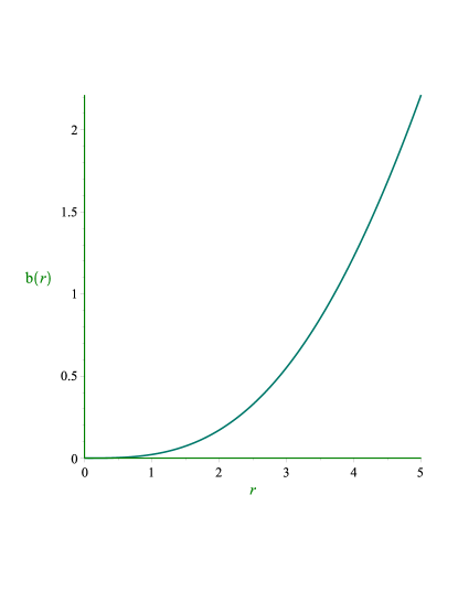
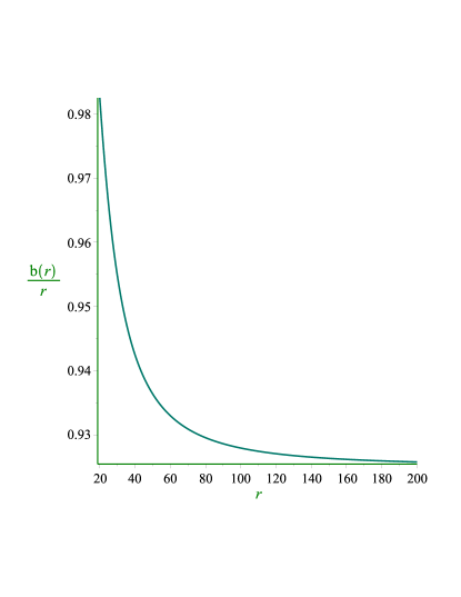
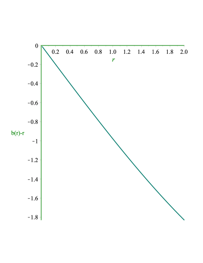
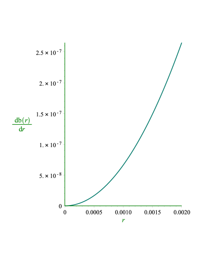
Figure 1: Graphs of $b(\emph{r})$, $\frac{b(\emph{r})}{\emph{r}}$, $b(\emph{r})-\emph{r}$ and $\frac{db(\emph{r})}{\emph{r}}$ corresponding to r for $\emph{c}_{2}$=30, $\emph{c}_{4}$=-0.0095 and h=-0.08.

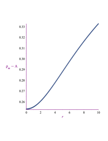
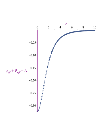
Figure 2: Graphs of $\rho_{m}-\textit{A}$ and $\mathrm{\rho}_{eff}+\mathrm{p}_{eff}-\textit{A}$ versus r

Case II: $\lambda(r)=-\frac{h}{\emph{r}}$

Here, Eq.(53) yields

$$\vartheta(r) = 2\ln\left\{-\left(\left(\emph{r}^{6}e^{\frac{h}{\emph{r}}}+8\emph{r}^{4}\emph{c}_{2}^{2}\emph{c}_{4}+8\emph{r}^{3}h\emph{c}_{2}^{2}\emph{c}_{4}+16\emph{r}^{2}\emph{c}_{2}^{2}\right.\right.\right.$$ (58)

$$+ \left.\left.\left.16\emph{r}h\emph{c}_{2}^{2}\right)^{\frac{1}{2}}+r^{3}e^{\frac{h}{2\emph{r}}}\right)\left(2\emph{c}_{2}\left(\emph{r}^{2}\emph{c}_{4}+2\right)\right)^{-1}\right\}.$$

The associated shape function becomes

$$b(r) = 2\emph{r}^{2}\left(\sqrt{\emph{r}^{6}e^{\frac{h}{\emph{r}}}+8\emph{r}^{4}\emph{c}_{2}^{2}\emph{c}_{4}+8\emph{r}^{3}h\emph{c}_{2}^{2}\emph{c}_{4}+16\emph{r}^{2}\emph{c}_{2}^{2}+16\emph{r}h\emph{c}_{2}^{2}}\right.$$

$$\times \left.\emph{r}e^{\frac{h}{2\emph{r}}}+\emph{r}^{5}e^{\frac{h}{\emph{r}}}+4h\emph{r}^{2}\emph{c}_{2}^{2}\emph{c}_{4}-4\emph{r}^{3}\emph{c}_{2}^{2}\emph{c}_{4}-2\emph{r}^{5}\emph{c}_{2}^{2}\emph{c}_{4}^{2}+8h\emph{c}_{2}^{2}\right)$$

$$\times \Big{\{}\left(\left(\emph{r}^{6}e^{\frac{h}{\emph{r}}}+8\emph{r}^{4}\emph{c}_{2}^{2}\emph{c}_{4}+8\emph{r}^{3}h\emph{c}_{2}^{2}\emph{c}_{4}+16\emph{r}^{2}\emph{c}_{2}^{2}+16\emph{r}h\emph{c}_{2}^{2}\right)^{\frac{1}{2}}\right.$$

$$+ \left.\emph{r}^{3}e^{\frac{h}{2\emph{r}}}\right)^{2}\Big{\}}^{-1}.$$

The corresponding energy density takes the form

$$\mathcal{\rho}_{m}=\sqrt{\frac{e^{\frac{-\lambda}{2}-\ln\left\{-\left(\emph{r}^{6}e^{\frac{h}{\emph{r}}}+8\emph{r}^{4}\emph{c}_{2}^{2}\emph{c}_{4}+8\emph{r}^{3}h\emph{c}_{2}^{2}\emph{c}_{4}+16\emph{r}^{2}\emph{c}_{2}^{2}+16\emph{r}h\emph{c}_{2}^{2}\right)^{\frac{1}{2}}-\emph{r}^{3}e^{\frac{h}{2\emph{r}}}\right\}}}{4\emph{c}_{2}^{2}\emph{c}_{3}\left(2+\emph{r}^{2}\emph{c}_{4}\right)}}.$$

Figure 3 indicates that the shape function maintains its positivity and the structure of WH is obtained asymptotically flat. The left graph in the lower panel exhibits the throat of WH at $\emph{r}_{0}=0.4$ and the associated right graph implies that $\frac{db\left(\emph{r}_{0}\right)}{d\emph{r}}<1$. For the existence of physically viable WH, we substitute the value of $\lambda(\emph{r})$ and $\vartheta(\emph{r})$ in Eq.(12), it gives

$$\mathrm{\rho}_{eff}+\mathrm{p}_{eff}-\textit{A} = \left(64\emph{c}_{2}^{2}+32\emph{r}^{2}\emph{c}_{2}^{2}\emph{c}_{4}\right)\left(4h^{2}\emph{r}^{2}\emph{c}_{2}^{2}\emph{c}_{4}-4h\emph{r}^{3}\emph{c}_{2}^{2}\emph{c}_{4}\right.$$

$$- \left.4\emph{r}^{4}\emph{c}_{2}^{2}\emph{c}_{4}+\emph{r}^{4}h^{2}\emph{c}_{2}^{2}\emph{c}_{4}^{2}-2\emph{r}^{6}\emph{c}_{2}^{2}\emph{c}_{4}^{2}-2h\emph{r}^{5}\emph{c}_{2}^{2}\emph{c}_{4}^{2}\right.$$

$$+ \left.4h^{2}\emph{c}_{2}^{2}+\emph{r}^{6}e^{\frac{h}{\emph{r}}}\right)+e^{\frac{h}{2\emph{r}}}\emph{r}^{3}\left(8\emph{r}^{4}\emph{c}_{2}^{2}\emph{c}_{4}+8\emph{r}^{3}h\emph{c}_{2}^{2}\emph{c}_{4}\right.$$

$$+ \left.\emph{r}^{6}e^{\frac{h}{\emph{r}}}+16\emph{r}^{2}\emph{c}_{2}^{2}+16\emph{r}h\emph{c}_{2}^{2}\right)^{\frac{1}{2}}\Big{\{}\left(\left(r^{6}e^{\frac{h}{r}}+16r^{2}\emph{c}_{2}^{2}\right.\right.$$

$$+ \left.\left.8\emph{r}^{4}\emph{c}_{2}^{2}\emph{c}_{4}+8\emph{r}^{3}h\emph{c}_{2}^{2}\emph{c}_{4}+16\emph{r}h\emph{c}_{2}^{2}\right)^{\frac{1}{2}}+r^{3}e^{\frac{h}{2\emph{r}}}\right)^{3}$$

$$\times \left(8\emph{r}^{4}\emph{c}_{2}^{2}\emph{c}_{4}+8\emph{r}^{3}h\emph{c}_{2}^{2}\emph{c}_{4}+\emph{r}^{6}e^{\frac{h}{\emph{r}}}+16\emph{r}^{2}\emph{c}_{2}^{2}\right.$$

$$+ \left.16\emph{r}h\emph{c}_{2}^{2}\right)^{\frac{1}{2}}\Big{\}}^{-1}.$$

Figure 4 implies that $\rho_{m}-\textit{A}\geq 0$ and $\mathrm{\rho}_{eff}+\mathrm{p}_{eff}-\textit{A}\leq 0$. This inequality assures the presence of a viable traversable wormhole.

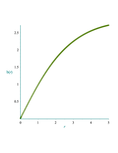
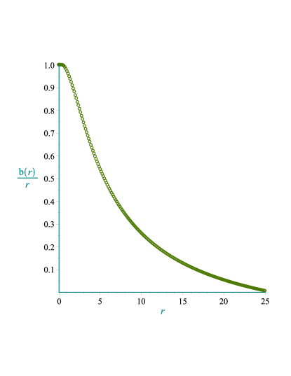
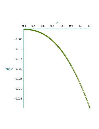
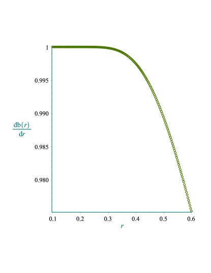
Figure 3: Graphs of $b(\emph{r}),~{}\frac{b(\emph{r})}{\emph{r}},~{}b(\emph{r})-\emph{r}$ and $\frac{db(\emph{r})}{\emph{r}}$ corresponding to r for $\emph{c}_{2}$=0.5=$\emph{c}_{3}$, $\emph{c}_{4}$=2.2 and h=4.9.

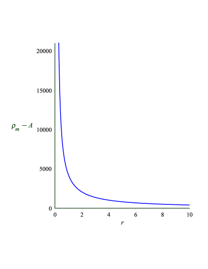
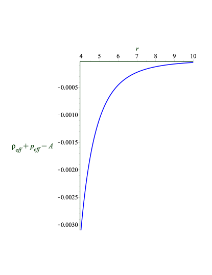
Figure 4: Graphs of $\rho_{m}-\textit{A}$ and $\mathrm{\rho}_{eff}+\mathrm{p}_{eff}-\textit{A}$ versus r

4.2 Non-Dust Case

In the presence of radiations, this case well explains the cosmic matter configuration. Therefore, we take into account a specific correlation between matter variables such that $\mathrm{p}_{m}(\lambda,\vartheta,\mathrm{M})=\omega\mathrm{\rho}_{m}(\lambda,\vartheta,\mathrm{M})$($\omega$ represents the equation of state parameter) and manipulate Eq.(48) which gives

$$\mathrm{\rho}_{m}=\frac{-\emph{c}_{2}\omega+\sqrt{\emph{c}_{2}^{2}\omega^{2}+4\emph{c}_{2}\emph{c}_{3}e^{\frac{-\lambda-\vartheta}{2}}+12\emph{c}_{2}\emph{c}_{3}\omega^{2}e^{\frac{-\lambda-\vartheta}{2}}}}{2\emph{c}_{2}\emph{c}_{3}\left(3\omega^{2}+1\right)}.$$ (59)

In this case, the generators of Noether symmetry are the same as for the dust case while the associated conserved quantities are given as

$$I_{1} = e^{\frac{\lambda-\vartheta}{2}}\emph{r}^{2}\bigg{\{}2\left(\frac{1+\lambda^{\prime}\emph{r}}{\emph{r}^{2}}\right)-e^{\vartheta}\left(\emph{c}_{4}+\frac{2}{\emph{r}^{2}}+\left(\emph{c}_{3}\left(3\omega^{2}+1\right)\right)\right.$$

$$\times \left.\left(\frac{-\emph{c}_{2}\omega+\sqrt{\emph{c}_{2}^{2}\omega^{2}+4\emph{c}_{2}\emph{c}_{3}e^{\frac{-\lambda-\vartheta}{2}}+12\emph{c}_{2}\emph{c}_{3}\omega^{2}e^{\frac{-\lambda-\vartheta}{2}}}}{2\emph{c}_{2}\emph{c}_{3}\left(3\omega^{2}+1\right)}\right)^{2}\right.$$

$$+ \left.\omega\frac{-\emph{c}_{2}\omega+\sqrt{\emph{c}_{2}^{2}\omega^{2}+4\emph{c}_{2}\emph{c}_{3}e^{\frac{-\lambda-\vartheta}{2}}+12\emph{c}_{2}\emph{c}_{3}\omega^{2}e^{\frac{-\lambda-\vartheta}{2}}}}{2\emph{c}_{2}\emph{c}_{3}\left(3\omega^{2}+1\right)}\right)\bigg{\}}$$

$$I_{2} = \emph{r}-\emph{c}_{2}\emph{r}e^{\frac{\lambda-\vartheta}{2}}\bigg{\{}\frac{2\lambda^{\prime}}{\emph{r}}+\frac{2}{\emph{r}^{2}}-e^{\vartheta}\left(\emph{c}_{4}+\frac{2}{\emph{r}^{2}}+\left(\emph{c}_{3}\left(3\omega^{2}+1\right)\right)\right.$$

$$\times \left.\left(\frac{-\emph{c}_{2}\omega+\sqrt{\emph{c}_{2}^{2}\omega^{2}+4\emph{c}_{2}\emph{c}_{3}e^{\frac{-\lambda-\vartheta}{2}}+12\emph{c}_{2}\emph{c}_{3}\omega^{2}e^{\frac{-\lambda-\vartheta}{2}}}}{2\emph{c}_{2}\emph{c}_{3}\left(3\omega^{2}+1\right)}\right)^{2}\right.$$

$$+ \left.\omega\frac{-\emph{c}_{2}\omega+\sqrt{\emph{c}_{2}^{2}\omega^{2}+4\emph{c}_{2}\emph{c}_{3}e^{\frac{-\lambda-\vartheta}{2}}+12\emph{c}_{2}\emph{c}_{3}\omega^{2}e^{\frac{-\lambda-\vartheta}{2}}}}{2\emph{c}_{2}\emph{c}_{3}\left(3\omega^{2}+1\right)}\right)\bigg{\}}$$

Substituting the values of matter variables from the equation of state and using Eq.(59) in (23), we obtain

$$e^{\vartheta(\emph{r})}=\frac{2+2\lambda^{\prime}\emph{r}}{\emph{r}^{2}\left(\emph{c}_{4}+\frac{2}{\emph{r}^{2}}+\frac{e^{\frac{-\lambda-\vartheta}{2}}}{\emph{c}_{2}}\right)}.$$ (60)

We study the structure and existence of viable WH for the same red-shift functions as discussed for the dust case.

Case I: $\lambda(r)=h$

In this case, Eq.(60) reduces to

$$\vartheta(\emph{r})=2\ln\bigg{\{}\frac{-\emph{r}^{2}e^{\frac{-h}{2}}+\sqrt{\left(e^{\frac{-h}{2}}\right)^{2}\emph{r}^{4}+8\emph{r}^{2}\emph{c}_{2}^{2}\emph{c}_{4}+16\emph{c}_{2}^{2}}}{2\emph{c}_{2}\left(r^{2}\emph{c}_{4}+2\right)}\bigg{\}}.$$ (61)

The corresponding shape function becomes

$$b(\emph{r}) = \bigg{\{}2\emph{r}^{3}\left(\emph{r}^{2}e^{-h}-4\emph{c}_{2}^{2}\emph{c}_{4}-e^{\frac{-h}{2}}\sqrt{\emph{r}^{4}e^{-h}+8\emph{r}^{2}\emph{c}_{2}^{2}\emph{c}_{4}+16\emph{c}_{2}^{2}}\right)$$

$$- 2\emph{r}^{2}\emph{c}_{2}^{2}\emph{c}_{4}^{2}\bigg{\}}\bigg{\{}\left(\emph{r}^{2}e^{\frac{-h}{2}}-\sqrt{\emph{r}^{4}e^{-h}+8\emph{r}^{2}\emph{c}_{2}^{2}\emph{c}_{4}+16\emph{c}_{2}^{2}}\right)^{2}\bigg{\}}^{-1}.$$

Inserting Eq.(61) in (59), we have

$$\mathrm{\rho}_{m} = \bigg{\{}-\emph{c}_{2}\omega+\bigg{\{}4\emph{c}_{2}\emph{c}_{3}e^{\frac{-\lambda}{2}-\ln\big{(}\frac{-\emph{r}^{2}e^{\frac{-h}{2}}+\sqrt{\left(e^{\frac{-h}{2}}\right)^{2}\emph{r}^{4}+8\emph{r}^{2}\emph{c}_{2}^{2}\emph{c}_{4}+16\emph{c}_{2}^{2}}}{2\emph{c}_{2}\left(\emph{r}^{2}\emph{c}_{4}+2\right)}\big{)}}$$

$$+ 12\emph{c}_{2}\emph{c}_{3}\omega^{2}e^{\frac{-\lambda}{2}-\ln\Big{(}\frac{-\emph{r}^{2}e^{\frac{-h}{2}}+\sqrt{\left(e^{\frac{-h}{2}}\right)^{2}\emph{r}^{4}+8\emph{r}^{2}\emph{c}_{2}^{2}\emph{c}_{4}+16\emph{c}_{2}^{2}}}{2\emph{c}_{2}\left(\emph{r}^{2}\emph{c}_{4}+2\right)}\big{)}}$$

$$+ \emph{c}_{2}^{2}\omega^{2}\bigg{\}}^{\frac{1}{2}}\bigg{\}}\left\{2\emph{c}_{2}\emph{c}_{3}\left(3\omega^{2}+1\right)\right\}^{-1}.$$

Figure 5 shows that upper face of the shape function remains positive but the structure of WH is not asymptotically flat. In the lower plane, WH throat is identified at $r_{0}=0.1$ and the associated right plot leads to $\frac{db\left(r_{0}\right)}{dr}<1$. Using Eq.(61) in Eq.(12), we have

$$\mathrm{\rho}_{eff}+\mathrm{p}_{eff}-\textit{A}=\frac{\emph{r}b^{\prime}-b}{\emph{r}^{3}}.$$

Figure 6 indicates that $\rho_{m}-\textit{A}\geq 0$ and $\mathrm{\rho}_{m}+\mathrm{p}_{m}-\textit{A}\geq 0$ for $0\leq\omega\leq 1$ while $\mathrm{\rho}_{eff}+\mathrm{p}_{eff}-\textit{A}\leq 0$ for $-1\leq\omega\leq 1$ which implies that viable traversable wormhole solution exists in this particular range of $\omega$.

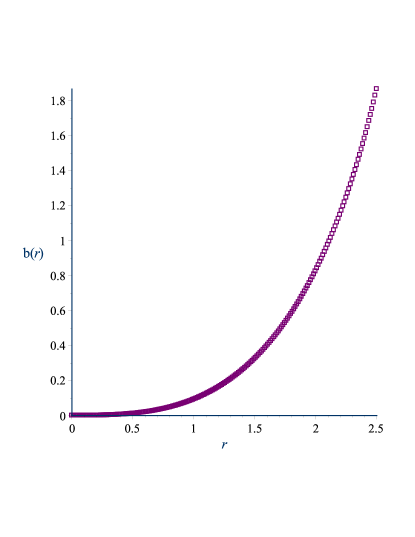
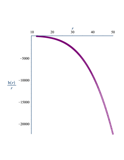
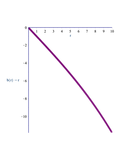
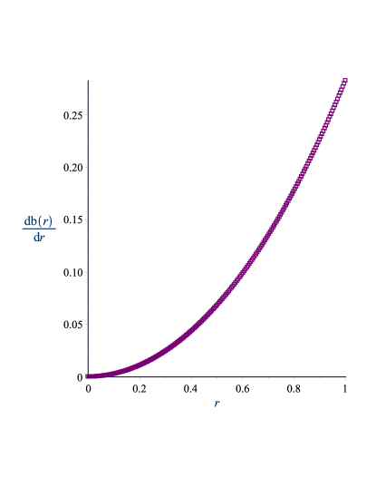
Figure 5: Graphs of $b(\emph{r})$, $\frac{b(\emph{r})}{\emph{r}}$, $b(\emph{r})-\emph{r}$ and $\frac{db(\emph{r})}{\emph{r}}$ corresponding to r for $\emph{c}_{2}$=5, $\emph{c}_{4}$=-0.3 and h=1.

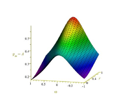
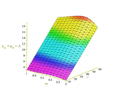
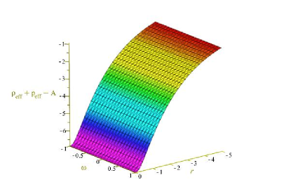
Figure 6: Graps of $\mathrm{\rho}_{m}-\textit{A}$, $\mathrm{\rho}_{m}+\mathrm{p}_{m}-\textit{A}$ and $\mathrm{\rho}_{eff}+\mathrm{p}_{eff}-\textit{A}$ corresponding to r.

Case II: $\lambda(r)=-\frac{h}{\emph{r}}$

Here, Eq.(60) leads to

$$\vartheta(\emph{r}) = 2\ln\bigg{\{}\left\{-\emph{r}^{3}e^{\frac{h}{2\emph{r}}}+\left(\emph{r}^{6}e^{\frac{h}{\emph{r}}}+8h\emph{r}^{3}\emph{c}_{2}^{2}\emph{c}_{4}+8r^{4}\emph{c}_{2}^{2}\emph{c}_{4}\right.\right.$$ (62)

$$+ \left.\left.16h\emph{r}\emph{c}_{2}^{2}+16\emph{r}^{2}\emph{c}_{2}^{2}\right)^{\frac{1}{2}}\right\}\left\{2\emph{c}_{2}\left(\emph{r}^{2}\emph{c}_{4}+2\right)\right\}^{-1}\bigg{\}}.$$

The associated shape function is

$$b(\emph{r}) = \bigg{\{}\left(\emph{r}^{5}e^{\frac{h}{\emph{r}}}+4h\emph{r}^{2}\emph{c}_{2}^{2}\emph{c}_{4}+8h\emph{c}_{2}^{2}-2\emph{r}^{5}\emph{c}_{2}^{2}\emph{c}_{4}^{2}-4\emph{r}^{3}\emph{c}_{2}^{2}\emph{c}_{4}\right.$$

$$- \left.\sqrt{\emph{r}^{6}e^{\frac{h}{\emph{r}}}+8h\emph{r}^{3}\emph{c}_{2}^{2}\emph{c}_{4}+8\emph{r}^{4}\emph{c}_{2}^{2}\emph{c}_{4}-16h\emph{r}\emph{c}_{2}^{2}+16\emph{r}^{2}\emph{c}_{2}^{2}}\right.$$

$$\times \left.\emph{r}^{2}e^{\frac{h}{2\emph{r}}}\right)2\emph{r}^{2}\bigg{\}}\setminus\bigg{\{}\left(8h\emph{r}^{3}\emph{c}_{2}^{2}\emph{c}_{4}+8\emph{r}^{4}\emph{c}_{2}^{2}\emph{c}_{4}-16h\emph{r}\emph{c}_{2}^{2}+\emph{r}^{2}\right.$$

$$\times \left.16\emph{c}_{2}^{2}+\emph{r}^{6}e^{\frac{h}{\emph{r}}}\right)^{\frac{1}{2}}-\emph{r}^{3}e^{\frac{h}{2\emph{r}}}\bigg{\}}^{2}.$$

Figure 7 shows that $b(r)$ remains positive but the geometry of WH is not asymptotically flat and WH throat is located at $\emph{r}_{0}=2$ with $\frac{db\left(\emph{r}_{0}\right)}{d\emph{r}}<1$. Figure 8 exhibits that $\rho_{m}-\textit{A}\geq 0$ and $\mathrm{\rho}_{m}+\mathrm{p}_{m}-\textit{A}\geq 0$ for $-1\leq\omega\leq 1$ whereas $\mathrm{\rho}_{eff}+\mathrm{p}_{eff}-\textit{A}<0$ for $-1\leq\omega\leq 0$, implying that physically viable and traversable WH exists.

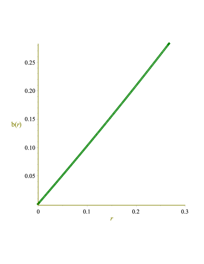
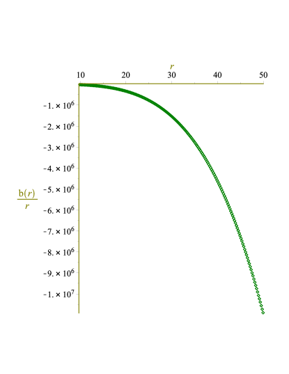
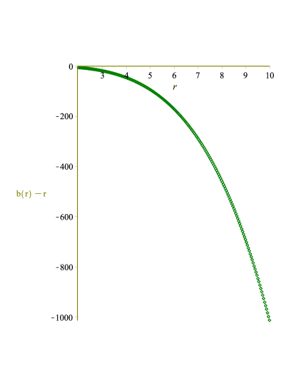
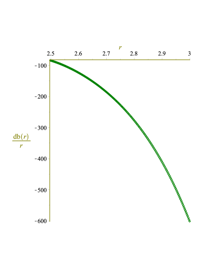
Figure 7: Graphs of $b(\emph{r})$, $\frac{b(\emph{r})}{\emph{r}}$, $b(\emph{r})-\emph{r}$ and $\frac{db(\emph{r})}{\emph{r}}$ corresponding to r for $\emph{c}_{2}$=0.4, $\emph{c}_{4}$=0.2 and h=-5.

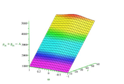
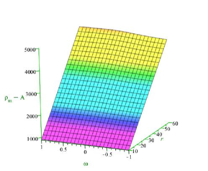
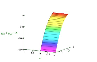
Figure 8: Graphs of $\mathrm{\rho}_{m}-\textit{A}$, $\mathrm{\rho}_{m}+\mathrm{p}_{m}-\textit{A}$ and $\mathrm{\rho}_{eff}+\mathrm{p}_{eff}-\textit{A}$ corresponding to r.

5 Stability Analysis

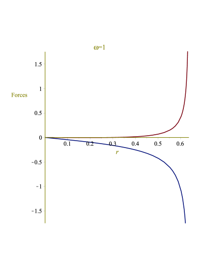
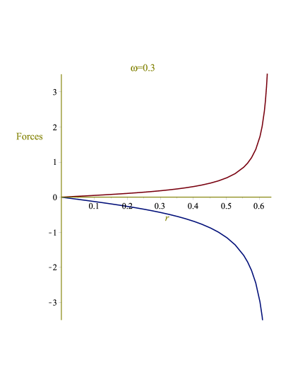
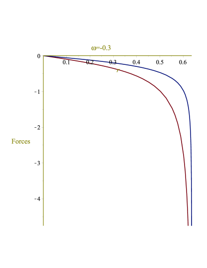
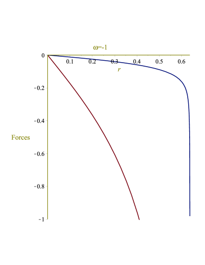
Figure 9: Graphs of $\mathcal{F}_{g}$ (red) and $\mathcal{F}_{\mathfrak{h}}$ (blue) versus r for constant red-shift function with $\emph{c}_{2}$=-0.5, $\emph{c}_{3}$=0.1, $\emph{c}_{4}$=-5 and h=1.

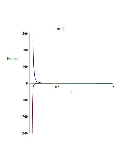
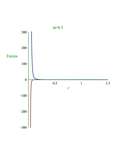
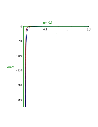
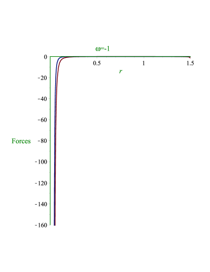
Figure 10: Graphs of $\mathcal{F}_{g}$ (red) and $\mathcal{F}_{\mathfrak{h}}$ (blue) versus r for variable red-shift function with $\emph{c}_{2}$=-8, $\emph{c}_{3}$=0.9, $\emph{c}_{4}$=-0.9 and h=0.5.

Here, we investigate the stability of viable and traversable WH solutions for both choices of red-shift function by using the TOV equation. We take into account non-conserved stress-energy tensor and formulate TOV equation for isotropic matter configuration as

$$\mathrm{p}_{m}^{\prime}+f_{\mathbf{T}^{2}}\left\{\left(3\mathrm{p}_{m}\mathrm{p}_{m}^{\prime}+\mathrm{\rho}_{m}\mathrm{\rho}_{m}^{\prime}\right)+\frac{\lambda^{\prime}}{2}\left(3\mathrm{p}_{m}^{2}+\mathrm{\rho}_{m}^{2}+4\mathrm{p}_{m}\mathrm{\rho}_{m}\right)\right\}+\frac{\lambda^{\prime}}{2}\left(\mathrm{\rho}_{m}+\mathrm{p}_{m}\right)=0.$$ (63)

This equation demonstrates the combination of gravitational force $\left(\mathcal{F}_{g}\right)$ and hydrostatic force $\left(\mathcal{F}_{h}\right)$ that determine the equilibrium state of WH. In the light of Eq.(63), these forces defined as

$$\mathcal{F}_{\mathfrak{h}}=\mathrm{p}_{m}^{\prime}\left(1+3\mathrm{p}_{m}f_{\mathbf{T}^{2}}\right),$$ (64)

$$\mathcal{F}_{g}=\frac{\lambda^{\prime}}{2}\left\{\left(\mathrm{\rho}_{m}+\mathrm{p}_{m}\right)+f_{\mathbf{T}^{2}}\left(3\mathrm{p}_{m}^{2}+\mathrm{\rho}_{m}^{2}+4\mathrm{p}_{m}\mathrm{\rho}_{m}\right)+f_{\mathbf{T}^{2}}\mathrm{\rho}_{m}\mathrm{\rho}_{m}^{\prime}\right\}.$$ (65)

The null impact of these forces $\left(\mathcal{F}_{\mathfrak{h}}+\mathcal{F}_{g}=0\right)$ ensure the presence of stable traversable WH. Figure 9 shows the stable and unstable behavior of viable traversable WH with constant red-shift function at distinct evolutionary eras. In the upper face, both plots indicate the stable state of WH for $\omega=1$ and $\omega=0.3$. This exhibits that WH preserves its stable state in the stiff matter era that remains until the radiation dominated era. The paths of both forces in the lower face are identical in direction as well as magnitude and hence violates the condition of equilibrium for both $\omega=-1$ and $\omega=-0.3$. This leads to the presence of stable and realistic traversable WH in the decelerating era whereas this stable state is disturbed in the cosmic accelerated expansion phase. For $\lambda(\emph{r})=\frac{-h}{\emph{r}}$, Eqs.(55) and (64) describe the stable state of WH incorporating with stiff matter, radiation dominated era and dark energy phase. The upward and downward faces of Figure 10 explain the fate of traversable WH such that in the decelerating phase it admits stable state whereas unstable state occurs in DE era.

6 Concluding Remarks

Noether symmetries are not just a mechanism to deal with the dynamical solutions, but also their possible existence may provide some feasible conditions so that one can choose some viable universe models according to recent observations. Lagrangian multipliers are useful to re-shape the Lagrangian into its canonical form which may prove to be quite useful to reduce the dynamics of the system and eventually help in determining the exact solutions. The existence of Noether charges are considered important in the literature and conserved quantities play an important role to analyze the mysterious universe.

The main challenge whether a WH exists is usually based on energy conditions which appears to be a fascinating subject in gravitation. In GR, the fundamental constituent for the existence of physically viable WH is the violation of energy conditions due to the presence of exotic matter. Modified gravitational theories have received significant attention as a possible alternative to GR during the last few decades. Many researchers found this quite significant to examine whether different modified theories violate the energy conditions by the effective energy-momentum tensor which leads to exotic matter and hence confirms the existence of a physically viable WH.

In this paper, we have used the Noether symmetry technique to evaluate some exact solutions that help to construct static WHs in EMSG and also investigate whether ordinary matter assists WHs or not in this theory. We have discussed the presence of exotic and normal matter in WHs through effective and ordinary energy bounds. We have taken a minimal coupling model to examine the viable WH geometry for both dust as well as non-dust matter distribution. We have also checked the stable and unstable states of these WH solutions through the TOV equation. We have formulated the complicated system through the Noether symmetry technique and determined the generators of symmetry with corresponding conserved quantities in the presence of shape function and energy density.

For EMSG model, we have examined the viability of WH solutions with red-shift functions $\lambda(\emph{r})=h$ and $\lambda(\emph{r})=-\frac{h}{\emph{r}}$ for dust as well as non-dust matter distribution and evaluated exact solutions. It is found that for $\lambda(\emph{r})=h$, WH fulfills all the necessary conditions for dust fluid while for non-dust distribution, WH does not preserve asymptotically flat behavior. The energy density for normal matter in both cases remains positive whereas the effective stress-energy tensor violates the $\mathbb{NEC}$. This implies that traversable WH exists whereas the existence of normal matter gives physically realistic WH. For $\lambda(\emph{r})=-\frac{h}{\emph{r}}$, all necessary conditions of WHs are satisfied for both matter distributions and specific relation between matter variables is considered in non-dust case ($\mathrm{p}_{m}=\omega\mathrm{\rho}_{m}$). For both matter distributions, we have found $\mathrm{\rho}_{m}-\textit{A}\geq 0$, $\mathrm{\rho}_{m}+\mathrm{p}_{m}-\textit{A}\geq 0$ and $\mathrm{\rho}_{eff}+\mathrm{p}_{eff}-\textit{A}\leq 0$. These inequalities indicate the presence of physically viable and traversable WH. Finally, we have checked the stability of WH against stiff matter-dominated and radiation-dominated era for both values of the red-shift function. This stable state of WHs becomes unstable as the universe passes through dust dominated phase and enters into the dark energy era.

Lobo and Oliveira [35] discussed the WH geometry in $f(R)$ gravity and found that no viable wormhole solution exists for the vacuum case. Zubair et al. [36] found static WH solutions with anisotropic, isotropic, and barotropic matter contents in $f(R,T)$ gravity. For this purpose, they considered a generalization of Starobinsky $f(R)$ model with linear form of $f(T)$ and tackled complexity of the field equations via numerical approach. To analyze the physical viability of WHs, they constructed a graphical analysis of energy bounds for all considered fluids and found that WH solutions can be studied without evolving exotic matter in certain regions of spacetime. They concluded that WH solutions are realistic and stable only for anisotropic matter in $f(R,T)$ gravity. Shamir and Ahmad [37] obtained the WH solutions with anisotropic matter distribution in $f(G,T)$ gravity. They investigated some viable regions for the presence of traversable wormhole geometries. Sharif et al. [38] analyzed static WH solutions using the Noether symmetry technique in $f(G)$ gravity and found a stable structure for different cases of red-shift function.

Recently, Capozziello et al. [39] derived the exact traversable WH solutions as well as stable conditions in the absence of exotic matter in $f(R)$ theory and found that small deviation from GR give stable solutions. De Falco et al. [40] formulated the static spherically symmetric WH solutions in the same framework. It is interesting to mention here that for $\mathbf{T}^{2}=0$, our results reduce to $f(R)$ gravity. We conclude that EMSG leads to the presence of more viable and stable WH solutions for isotropic matter configuration through Noether symmetry approach.

References

[1] Felice, A.D. and Tsujikawa, S.R.: Living Rev. Relativ.
13(2010)3; Nojiri, S. and Odintsov, S.D.: Phys. Rep.
505(2011)59; Bamba, et al.: Astrophys. Space Sci.
342(2012)155.
[2] Harko, T. et al.: Phys. Rev. D 84(2011)024020.
[3] Haghani, Z. et al.: Phys. Rev. D 88(2013)044023.
[4] Moraes, P.H.R.S. and Santos, J.R.L.: Eur. Phys. J. C 76(2016)60.
[5] Katirci, N. and Kavuk, M.: Eur. Phys. J. Plus 129(2014)163.
[6] Chen, C.Y. and Chen, P.: Phys. Rev. D 101 (2020)064021;
Bhattacharjee, S. and Sahoo, P.K.: Eur. Phys. J. Plus 135
(2020)86; Barbar, A.H., Awad, A.M. and AlFiky, M.T.: Phys. Rev. D
101 (2020)044058; Sharif, M. and Gul, M.Z.: Phys. Scr.
96(2020)025002.
[7] Board, C.V.R. and Barrow, J.D.: Phys. Rev. D 96(2017)123517.
[8] Nari, N. and Roshan, M.: Phys. Rev. D 98(2018)024031.
[9] Moraes P.H.R.S. and Sahoo, P.K.: Phys. Rev. D 97 (2018)024007.
[10] Bahamonde, S., Marciu, M. and Rudra, P.: Phys. Rev. D 100
(2019)083511.
[11] Sharif, M. and Gul M.Z.: Phys. Scr.
96(2020)025002; Int. J. Mod. Phys. A
36(2021)2150004; Chin. J. Phys. 71(2021)365.
[12] Demianski, et al.: Phys. Rev. D 46(1992)1391.
[13] Capozziello, S., Stabile, A. and Troisi, A.: Class. Quantum Grav.
24(2007)2153; ibid. 25(2008)085004; ibid.
27(2010)165008.
[14] Shamir, M.F., Jhangeer, A. and Bhatti, A.A.: Chin. Phys. Lett. 29(2012)080402.
[15] Kucukakca, Y., Camci, U. and Semiz, I.: Gen. Relativ. Gravit. 44(2012)1893.
[16] Sharif, M. and Waheed, S.: Can. J. Phys. 88(2010)833;
Phys. Scr. 83(2011)015014; J. Cosmol. Astropart. Phys.
2(2013)043; Sharif, M. and Nawazish, I.: J. Exp. Theor.
Phys. 120(2014)49; Sharif, M. and Shafique, I.: Phys. Rev.
D 90(2014)084033; Sharif, M. and Fatima, H.I.: J. Exp.
Theor. Phys. 122(2016)104; Sharif, M. and Gul, M.Z.: Eur.
Phys. J. Plus 133(2018)345; Int. J. Mod. Phys. D
28(2019)1950054; Chin. J. Phys. 57(2019)329.
[17] Kashargin, P.E. and Sushkov, S.V.: Gravit. Cosmol. 14(2008)80;
Eiroa, E.F. and Simeone, C.: Phys. Rev. D 82(2010)084039.
[18] Bahamonde, S. et al.: Phys. Rev. D 94(2016)044041.
[19] Sharif, M. and Fatima, I.: Gen. Relativ. Gravit. 48(2016)148;
ibid. 400(2019)37. Astrophys. Space Sci.
361(2016)127.
[20] Mazharimousavi, S.H. and Halilsoy, M.: Mod. Phys. Lett. A 31(2016)1650203.
[21] Bahamonde, S. et al.: Phys. Rev. D 94(2016)084042.
[22] Sharif, M. and Nawazish, I.: Ann. Phys 389(2018)283.
[23] Zubair, M., Waheed, S. and Ahmed, Y.: Eur. Phys. J. C 76(2016)444.
[24] Morris, M. and Thorne, A.: Am. J. Phys. 56(1988)395.
[25] Ellis, G.F.R. R., Maartens and MacCallum, M.A.H.: Relativistic Cosmology (Cambridge University Press, 2012).
[26] Carroll, S.: Spacetime and Geomety, An Introduction to General
Relativity (Addison Wesley, 2004).
[27] Santos, J. et al.: Phys. Rev. D 76(2007)083513.
[28] Capozziello, S., De Laurentis, M. and Odintsov, S.D.: Eur. Phys. J.
C 72(2012)1434.
[29] Basilakos, S. et al.: Phys. Rev. D 88(2013)103526.
[30] Paliathanasis, A. et al.: Phys. Rev. D 89(2014)063532.
[31] Paliathanasis, A., Tsamparlis, M. and Basilakos, S.: Phys. Rev. D
84(2011)123514.
[32] Basilakos, S., Tsamparlis, M. and Paliathanasis, A.:
Phys. Rev. D 83(2011)103512.
[33] Roshan, M. and Shojai, M.: Phys. Rev. D
94(2016)044002.
[34] Kar, S. and Sahdev, D.: Phys. Rev. D 52(1995)2030.
[35] Lobo, F.S.N. and Oliveira, M.A.: Phys. Rev. D 80(2009)104012.
[36] Zubair, M. Waheed, S. and Ahmed, Y.: Eur. Phys. J. C 76(2016)444.
[37] Shamir, M.F. and Ahmad, M.: Int. J. Geom. Methods Mod. Phys. 15(2018)1850070.
[38] Sharif, M., Nawazish, I. and Hussain, S.: Eur. Phys. J. C 80(2021)783.
[39] Capozziello, S., Luongo, O. and Mauro, L.: Eur. Phys. J. Plus 136(2021)167.
[40] De Falco, V. et al.: Eur. Phys. J. C 81(2021)157.