Topological Uncertainty: Monitoring trained neural networks
through persistence of activation graphs

Abstract

Although neural networks are capable of reaching astonishing performances on a wide variety of contexts, properly training networks on complicated tasks requires expertise and can be expensive from a computational perspective. In industrial applications, data coming from an open-world setting might widely differ from the benchmark datasets on which a network was trained. Being able to monitor the presence of such variations without retraining the network is of crucial importance. In this article, we develop a method to monitor trained neural networks based on the topological properties of their activation graphs. To each new observation, we assign a Topological Uncertainty, a score that aims to assess the reliability of the predictions by investigating the whole network instead of its final layer only, as typically done by practitioners. Our approach entirely works at a post-training level and does not require any assumption on the network architecture, optimization scheme, nor the use of data augmentation or auxiliary datasets; and can be faithfully applied on a large range of network architectures and data types. We showcase experimentally the potential of Topological Uncertainty in the context of trained network selection, Out-Of-Distribution detection, and shift-detection, both on synthetic and real datasets of images and graphs.

1 Introduction

Over the last decade, Deep Learning (DL) has become the most popular approach to tackle complex machine learning tasks, opening the door to a broad range of industrial applications. Despite its undeniable strengths, monitoring the behavior of deep Neural Networks (NN) in real-life applications can be challenging. The more complex the architectures become, the stronger the predictive strengths of the networks, but the looser our grasp on their behaviors and weaknesses.

Training a neural network requires task-specific expertise, is time consuming, and requires the use of high-end expensive hardware. With the rise of companies providing model marketplaces (e.g., (Kumar et al., 2020, §, Table 1) or tensorflow-hub), it is now common that users only have access to fixed trained neural networks, with few information on the training process, and would rather avoid training the networks again.

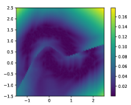
Figure 1: (Left) Confidence (maximum in the final soft-max layer) of the predictions made by a neural network trained on the two-moons dataset (white and black crosses) over the plane. Away from the thin classification boundary (confidence value close to $0.5$), the network tends to produce over-confident predictions (value close to $1$), even for points that are far away from the training data. (Right) Topological distance between all activation graphs and the activation graphs computed on the train set (higher means less confident).

In practice, a network can perform well on a given learning problem—in the sense that it can achieve high accuracy on the training and test sets—, but lack reliability when used in real-life applications thereafter. One can think of, among other examples, adversarial attacks, that are misinterpreted by neural networks with high confidence levels Nguyen et al. (2015); Akhtar and Mian (2018); Biggio and Roli (2018), calibration issues leading to under- or over-confident predictions Guo et al. (2017); Ovadia et al. (2019); Hein et al. (2019), lack of robustness to corruption or perturbation of the input data Hendrycks and Dietterich (2019).

Related work.

Many techniques have been proposed to improve or monitor the behavior of NN deployed in real-life applications. Most require specific actions taken during the training phase of the network; for instance via data augmentation Shorten and Khoshgoftaar (2019)), the use of large auxiliary datasets Hendrycks et al. (2019), modifications of the network architecture DeVries and Taylor (2018) or its objective function Atzmon et al. (2019); Van Amersfoort et al. (2020), or using several networks at once to produce predictions Lakshminarayanan et al. (2017). The approach we introduce in this article focuses on acting at a post-training level only, and since our goal is to benchmark it against the use of confidence alone in a similar setting, we use, in our experimental results, the baseline introduced in Hendrycks and Gimpel (2017), which proposes to monitor NNs based on their confidences and on the idea that low-confidence predictions may account for anomalies.

Using topological quantities to investigate NN properties has experienced a growth of interest recently (see for instance Guss and Salakhutdinov (2018); Carlsson and Gabrielsson (2020)). In Gebhart and Schrater (2017); Gebhart et al. (2019), the authors introduce the notion of activation graphs and showcase their use in the context of adversarial attacks. We mix this idea with Rieck et al. (2019), which proposes to investigate topological properties of NN layer-wise. A topological score based on an estimation of the NN decision boundary has been proposed in Ramamurthy et al. (2019) to perform trained network selection, an idea we adapt in Subsection 4.1.

Contributions.

In this work, we propose a new approach to monitor trained NNs by leveraging the topological properties of activation graphs. Our main goal is to showcase the potential benefits of investigating network predictions through the lens of the whole network instead of looking at its confidence encoded by its final layer only as usually done in practice.

To that aim, we introduce Topological Uncertainty (TU), a simple topological quantity that, for a given NN and a new observation, encodes how the network “reacts” to this observation, and whether this reaction is similar to the one on training data. Our approach does not require any assumption on the network training phase nor the type of input data, and can thus be deployed in a wide variety of settings. Furthermore, it only relies on computating maximum spanning trees (MST), leading to a simple and efficient implementation.

Experimentally, we show that TU can be used to monitor trained NNs and detect Out-of-Distribution (OOD) or shifted samples when deployed in real-life applications. Our results suggest that TU can drastically improve on a standard baseline based on the network confidence in different situations. Our implementation will be made publicly available.

2 Background

2.1 Neural networks

For the sake of clarity, we restrict our presentation to sequential neural networks, although our approach (detailed in Section 3) can be generalized to more general architectures, e.g., recurrent neural networks. We also restrict to classification tasks; let $d$ denote the dimension of the input space and $K$ be the number of classes. A (sequential) neural network (NN) learns a function $F\colon\mathbb{R}^{d}\to\mathbb{R}^{K}$ that can be written as $F=f_{L}\circ\dots\circ f_{1}$, where the $(f_{\ell})_{\ell=1}^{L}$ are elementary blocks defined for $\ell=1,\dots,L-1$ as

$$x_{\ell+1}=f_{\ell}(x_{\ell})=\sigma_{\ell}(W_{\ell}\cdot x_{\ell}+b_{\ell}),$$ (1)

with $W_{\ell}\in\mathbb{R}^{d_{\ell}\times d_{\ell+1}}$, $b_{\ell}\in\mathbb{R}^{d_{\ell+1}}$, and $(\sigma_{\ell})_{\ell}$ are activation maps, e.g., $\sigma_{\ell}=\mathrm{ReLU}\colon x\mapsto\max\{x,0\}$. In classification tasks, the final activation $f_{L}=\sigma_{L}$ is usually taken to be the soft-max function, so that the output $x_{L}=F(x)$ can be understood as a probability distribution on $\{1,\dots,K\}$ whose entries $(F(x)_{k})_{k}$ indicate the likelihood that $x$ belongs to class $k$. The predicted class is thus $\operatorname*{arg\,max}_{k}\{F(x)_{k}\}$, while the confidence that the network has in its prediction is $\max_{k}\{F(x)_{k}\}\in[0,1]$. Given a training set of observations and labels $(X^{\text{train}},Y^{\text{train}})=(x_{i},y_{i})_{i=1}^{N_{\mathrm{train}}}$ distributed according to some (unknown) joint law $(\mathcal{X},\mathcal{Y})$, the network parameters $W_{\ell},b_{\ell}$ are optimized to minimize the loss $\sum\mathcal{L}(F(x_{i}),y_{i})$ for some loss function $\mathcal{L}$ (e.g., the categorical cross-entropy). The (training) accuracy of $F$ is defined as $\frac{1}{N_{\mathrm{train}}}\sum_{i=1}^{N_{\mathrm{train}}}1_{\operatorname*{arg\,max}(F(x_{i}))=y_{i}}$.

2.2 Activation graphs and topological descriptors

Activation graphs.

Let us consider a neural network $F$ and two layers of size $d_{\ell}$ and $d_{\ell+1}$ respectively, connected by a matrix $W_{\ell}\in\mathbb{R}^{d_{\ell}\times d_{\ell+1}}$. One can build a bipartite graph $G_{\ell}$ whose vertex set is $V_{\ell}\sqcup V_{\ell+1}$ with $|V_{\ell}|=d_{\ell}$ and $|V_{\ell+1}|=d_{\ell+1}$, and edge set is $E_{\ell}=V_{\ell}\times V_{\ell+1}$. Following Gebhart et al. (2019), given an instance $x\in\mathbb{R}^{d}$, one can associate to each edge $(i,j)\in E_{\ell}$ the weight $|W_{\ell}(i,j)\cdot x_{\ell}(i)|$, where $x_{\ell}(i)$ (resp. $W_{\ell}(i,j)$) denotes the $i$-th coordinate of $x_{\ell}\in\mathbb{R}^{d_{\ell}}$ (resp. entry $(i,j)$ of $W_{\ell}\in\mathbb{R}^{d_{\ell}\times d_{\ell+1}}$). Intuitively, the quantity $|W_{\ell}(i,j)\cdot x_{\ell}(i)|$ encodes how much the observation $x$ “activates” the connection between the $i$-th unit of the $\ell$-th layer and the $j$-th unit of the $(\ell+1)$-th layer of $F$. In this way, we obtain a sequence of bipartite graphs $(G_{\ell}(x,F))_{\ell}$ called the activation graphs of the pair $(x,F)$, whose vertices are $V_{\ell}\sqcup V_{\ell+1}$ and edges weights are given by the aforementioned formula.

Maximum spanning trees and persistence diagrams.

To summarize the information contained in these possibly large graphs in a quantitative way, we rely on topological descriptors called persistence diagrams, coming from the Topological Data Analysis (TDA) literature. A formal introduction to TDA is not required in this work (we refer to the appendix for a more general introduction): in our specific case, persistence diagrams can be directly defined as the distribution of weights of a maximum spanning tree (MST). We recall that given a connected graph $G$ with $N+1$ vertices, a MST is a connected acyclic sub-graph of $G$ sharing the same set of vertices such that the sum of the $N$ edge weights is maximal among such sub-graphs. MST can be computed efficiently, namely in quasilinear time with respect to the number of edges in $G$. Given the ordered weights $w_{1}\geq\dots\geq w_{N}$ of a MST built on top of a graph $G$, its persistence diagram is the one-dimensional probability distribution

$$\mu(G):=\frac{1}{N}\sum_{i=1}^{N}\delta_{w_{i}},$$ (2)

where $\delta_{w_{i}}$ denotes the Dirac mass at $w_{i}\in\mathbb{R}$. See Figure 2 for an illustration.

Comparing and averaging persistence diagrams.

The standard way to compare persistence diagrams relies on optimal partial matching metrics. The choice of such metrics is motivated by stability theorems that, in our context, imply that the map $x\mapsto\mu(G_{\ell}(x,F))$ is Lipschitz with Lipschitz constant that only depends on the network architecture and weights (and not on properties of the distribution of $x\sim\mathcal{X}$ for instance). The computation of these metrics is in general challenging Kerber et al. (2017). However, in our specific setting, the distance $\mathrm{Dist}(\mu,\nu)$ between two diagrams $\mu=\frac{1}{N}\sum_{i=1}^{N}\delta_{w_{i}}$ and $\nu=\frac{1}{N}\sum_{j=1}^{N}\delta_{w^{\prime}_{j}}$ can be simply obtained by computing a 1D-optimal matching⁵, which in turn only requires to match points in increasing order, leading to the simple formula

$$\mathrm{Dist}(\mu,\nu)^{2}=\frac{1}{N}\sum_{i=1}^{N}|w_{i}-w^{\prime}_{i}|^{2},$$ (3)

where $w_{1}\geq w_{2}\geq\dots\geq w_{N}$ and $w^{\prime}_{1}\geq w^{\prime}_{2}\geq\dots\geq w^{\prime}_{N}$. With this metric comes a notion of average persistence diagram, called a Fréchet mean Turner et al. (2014): a Fréchet mean $\overline{\mu}$ of a set of $M$ diagrams $\mu_{1},\dots,\mu_{M}$ is a minimizer of $\nu\mapsto\sum_{m=1}^{M}\mathrm{Dist}(\mu_{m},\nu)^{2}$, which in our context simply reads

$$\overline{\mu}:=\frac{1}{N}\sum_{i=1}^{N}\delta_{\bar{w}_{i}},$$ (4)

where $\bar{w}_{i}=\frac{1}{M}\sum_{m=1}^{M}w_{i}^{(m)}$ and $w_{i}^{(m)}$ denotes the $i$-th point of $\mu_{m}$. The Fréchet mean provides a geometric way to concisely summarize the information contained in a set of persistence diagrams.

3 Topological Uncertainty (TU)

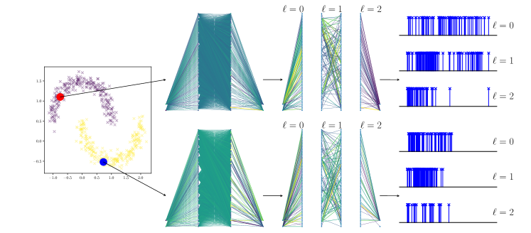
Figure 2: Pipeline presented in this article: Each observation activates the network with a weight $|W_{\ell}(i,j)\cdot x_{\ell}(i)|$ on the edge connecting the $i$-th unit in the $\ell$-th layer to the $j$-th unit of the $(\ell+1)$-th layer. A maximum spanning tree is then computed for each layer $\ell$ of the network, whose distribution of weights provides a corresponding persistence diagram. On this example, the network used is a simple network with two hidden-layers of 64 units each with ReLU activation, each layer is fully-connected (dense matrix).

Building on the material introduced in Section 2, we propose the following pipeline, which is summarized in Figure 2. Given a trained network $F$ and an observation $x$, we build a sequence of activation graphs $G_{1}(x,F),\dots,G_{L-1}(x,F)$. We then compute a MST of each $G_{\ell}(x,F)$, which in turn induces a persistence diagram $D_{\ell}(x,F):=\mu(G_{\ell}(x,F))$.

Topological Uncertainty.

Given a network $F\colon\mathbb{R}^{d}\to\mathbb{R}^{K}$ trained on a set $X^{\text{train}}$, one can store the corresponding sequence of diagrams $(D_{\ell}(x^{\text{train}},F))_{\ell}$ for each $x^{\text{train}}\in X^{\text{train}}$. These diagrams summarize how the network is activated by the training data. Thus, given a new observation $x$ with $\operatorname*{arg\,max}(F(x))=k$, one can compute the sequence $(D_{\ell}(x,F))_{\ell}$ and then the quantity

$$\min_{\begin{subarray}{c}x^{\text{train}}\in X^{\text{train}},\\ \operatorname*{arg\,max}(F(x^{\text{train}}))=k\end{subarray}}\mathrm{Dist}\left(D_{\ell}(x,F),D_{\ell}(x^{\text{train}},F)\right),$$ (5)

that is, comparing $D_{\ell}(x,F)$ to the diagrams of training observations that share the same predicted label than $x$. Figure 1 (right) shows how this quantity evolves over the plane, and how, contrary to the network confidence (left), it allows one to detect instances that are far away from the training distribution.

Since storing the whole set of training diagrams for each class and each layer $\{D_{\ell}(x^{\text{train}},F)\;:\;\operatorname*{arg\,max}(F(x^{\text{train}}))=k\}$ might be inefficient in practice, we propose to summarize these sets through their respective Fréchet means $\overline{D^{\text{train}}_{\ell,k}}$. For a new observation $x\in\mathbb{R}^{d}$, let $k(x)=\operatorname*{arg\,max}(F(x))$ be its predicted class, and $(D_{\ell}(x,F))_{\ell}$ the corresponding persistence diagrams. The Topological Uncertainty of $x$ is defined to be

$$\mathrm{TU}(x,F):=\frac{1}{L}\sum_{\ell=1}^{L}\mathrm{Dist}\left(D_{\ell}(x,F),\overline{D^{\text{train}}_{\ell,k(x)}}\right),$$ (6)

which is the average distance over layers between the persistence diagrams of the activation graphs of $(x,F)$ and the average diagrams stored from the training set. Having a low TU suggests that $x$ activates the network $F$ in a similar way to the points in $X^{\text{train}}$ whose class predicted by $F$ was the same as $x$. Conversely, an observation with a high TU (although being possibly classified with a high confidence) is likely to account for an OOD sample as it activates the network in an unusual manner.

Remarks.

Our definition of activation graphs differs from the one introduced in Gebhart et al. (2019), as we build one activation graph for each layer, instead of a single, possibly very large, graph on the whole network. Note also that the definition of TU can be declined in a variety of ways. First, one does not necessarily need to work with all layers $1\leq\ell\leq L$, but can only consider a subset of those. Similarly, one can estimate Fréchet means $\overline{D^{\text{train}}_{\ell,k}}$ using only a subset of the training data. These techniques might be of interest when dealing with large datasets and deep networks. One could also replace the Fréchet mean $\overline{D^{\text{train}}_{\ell,k}}$ by some other diagram of interest; in particular, using the empty diagram instead allows us to retrieve a quantity analog to the Neural persistence introduced in Rieck et al. (2019). On an other note, there are other methods to build persistence diagrams on top of activation graphs that may lead to richer topological descriptors, but our construction has the advantage of returning diagrams supported on the real line (instead of the plane as it usually occurs in TDA) with fixed number of points, which dramatically simplifies the computation of distances and Fréchet means, and makes the process efficient practically.

4 Experiments

This section showcases the use of TU in different contexts: trained network selection (§4.1), monitoring of trained networks that achieve large train and test accuracies but have not been tweaked to be robust to Out-Of-Distribution observations (§4.2) or distribution shift (§4.3).

Datasets and experimental setting.

We use standard, publicly available, datasets of graphs and images. MNIST, Fashion-MNIST, CIFAR-10, SVHN, DTD are datasets of images, while MUTAG and COX2 are datasets of graphs coming from a chemical framework. We also build two OOD image datasets, Gaussian and Uniform, by randomly sampling pixel values following a Gaussian distribution (resp. uniform on the unit cube). A detailed report of datasets and experimental settings (data preprocessing, network architectures and training parameters, etc.) can be found in the appendix.

4.1 Trained network selection for unlabeled data

In this subsection, we showcase our method in the context of trained network selection through an experiment proposed in (Ramamurthy et al., 2019, §4.3.2). Given a dataset with 10 classes (here, MNIST or Fashion-MNIST), we train $45$ NNs on the binary classification problems $i$ vs. $j$ for each pair of classes $(i,j)$ with $i>j$, and store the average persistence diagrams of the activation graphs for the different layers and classes as explained in Section 3. These networks are denoted by $F_{ij}$ in the following, and consistently reach high accuracies on their respective training and test sets given the simplicity of the considered tasks. Then, for each pair of classes $k_{1}>k_{2}$, we sample a set of new observations $X_{k_{1},k_{2}}$ made of $200$ instances sampled from the test set of the initial dataset (in particular, these observations have not been seen during the training of any of the $(F_{ij})_{ij}$) whose labels are $k_{1}$ and $k_{2}$. Assume now that $k_{1},k_{2}$ and the labels of our new observations are unknown. The goal is to select a network that is likely to perform well on $X_{k_{1},k_{2}}$ among the $(F_{ij})_{ij}$. To that aim, we compute a score for each pairing $(k_{1},k_{2})\leftrightarrow(i,j)$, which is defined as the average TU (see Eq. (6)) when feeding $F_{ij}$ with $X_{k_{1},k_{2}}$. A low score between $(i,j)$ and $(k_{1},k_{2})$ suggests that $X_{k_{1},k_{2}}$ activates $F_{ij}$ in a “known” way, thus that $F_{ij}$ is likely to be a relevant classifier for $X_{k_{1},k_{2}}$, while a high score suggests that the data in $X_{k_{1},k_{2}}$ is likely to be different from the one on which $F_{i,j}$ was trained, making it a less relevant choice. Figure 3 plots the couple (scores, accuracies) obtained on MNIST when taking $(k_{1},k_{2})=(1,0)$, that is, we feed networks that have been trained to classify between $i$ and $j$ handwritten digits with images representing $0$ and $1$ digits. Not surprisingly, $F_{1,0}$ achieves both a small TU (thus would be selected by our method) and a high accuracy. On the other hand, using the model $F_{7,6}$ on $X_{1,0}$ leads to the highest score and a low accuracy.

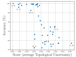
Figure 3: Score and accuracies obtained on 45 models trained on the MNIST dataset when fed with a set $X_{1,0}$ of images representing $0$ and $1$ digits. The point annotations refer to the values $(i,j)$ on which the network was initially trained. For instance, a network trained on $7$ and $4$ has a score of $0.49$ and an accuracy of $\sim 75$% on $X_{1,0}$.

To quantitatively evaluate the benefit of using our score to select a model, we use the the metric proposed by Ramamurthy et al. (2019): the difference between the mean accuracy obtained using the 5 models that have the lowest scores and the 5 models that have the highest scores. We obtain a $+14.8$%-increase on MNIST and a $+12.6$%-increase on Fashion-MNIST. These positive values indicate that, on average, using low TU as a criterion helps to select a better model to classify our new set of observations. As a comparison, using the average network confidence as a score leads to $+6.6\%$ on MNIST and $+4.7\%$ on Fashion-MNIST, indicating that using (high) confidence to select a model would be less relevant than using TU, on average. See the appendix for a complementary discussion.

Remark.

Our setting differs from the one of Ramamurthy et al. (2019): in the latter work, the method requires to have access to true labels on the set of new observations $X_{k_{1},k_{2}}$ (which we do not), but do not need to evaluate $F_{ij}(x),\ x\in X_{k_{1},k_{2}}$ on each model $F_{ij}$ (which we do). To that respect, we stress the complementary aspect of both methods.

4.2 Detection of Out-Of-Distribution samples

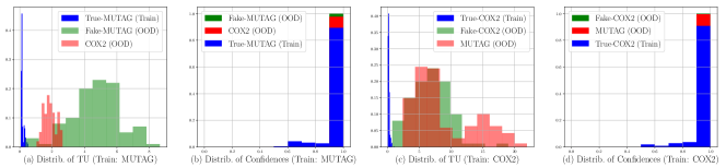
Figure 4: (a) Distributions of Topological Uncertainties (TU) of a network trained on the MUTAG dataset. Blue distribution corresponds to $\mathcal{T}^{\text{train}}$. Green and red distributions correspond to topological uncertainties of observations coming from Fake-MUTAG and COX2 datasets respectively. (b) Distributions of network confidences ($\max\{F(x)_{k}\}$). The network makes overconfident predictions, especially on OOD datasets that are classified almost systematically with a confidence of $1$. (c,d) Similar plots for the COX2 dataset.

The following experiment illustrates the behavior of TU when a trained network faces Out-Of-Distribution (OOD) observations, that is, observations that are not distributed according to the training distribution. To demonstrate the flexibility of our approach, we present the experiment in the context of graph classification, relying on the COX2 and the MUTAG graph datasets. Complementary results on image datasets can be found in Table 1 and in the appendix. Working with these datasets is motivated by the possibility of using simple networks while achieving reasonably high accuracies which are near state-of-the-art on these sets. To train and evaluate our networks, we extract $40$ spectral features from graphs—thus representing a graph by a vector in $\mathbb{R}^{40}$—following a procedure proposed in Carrière et al. (2020). See the appendix for details.

For both datasets, we build a set of 100 fake graphs in the following way. Let $\mathcal{N}$ and $\mathcal{M}$ be the distributions of number of vertices and number of edges respectively in a given dataset (e.g., graphs in MUTAG have on average $17.9\pm 4.6$ vertices and $19.8\pm 5.7$ edges). Fake graphs are sampled as Erdős-Renyi graphs of parameters $(n,m/n^{2})$, with $n\sim\mathcal{N}$, $m\sim\mathcal{M}$, thus by construction fake graphs have (on average) the same number of vertices and edges as graphs from the training dataset. These sets are referred to as Fake-MUTAG and Fake-COX2, respectively.

		Baseline		Topological Uncertainty
Training data	OOD data	FPR (TPR 95%) $\downarrow$	AUC $\uparrow$	FPR (TPR 95%) $\downarrow$	AUC $\uparrow$
MUTAG	Fake-MUTAG	98.4	1.7	0.0	99.8
	COX2	93.0	31	0.0	100.0
COX2	Fake-COX2	91.2	1.4	0.0	99.9
	MUTAG	91.2	1.1	0.0	100.0
CIFAR-10	FMNIST	93.6	54.9	65.6	86.4
	MNIST	94.7	58.3	25.4	94.7
	SVHN	90.6	27.6	83.6	65.8
	DTD	90.9	32.6	90.3	57.3
	Uniform	91.5	31.8	59.1	80.2
	Gaussian	91.0	27.2	18.8	88.2

Table 1: Comparison between the baseline OOD-detector based on network confidence and our TU-based classifier on graph datasets (first two rows) and on image datasets for a network trained on CIFAR-10 (third row). $\uparrow$: higher is better, $\downarrow$: lower is better.

Now, given a network $F_{\texttt{MUTAG}}$ trained on MUTAG (resp. $F_{\texttt{COX2}}$ trained on COX2), we store the average persistence diagrams of each classes. It allows us to compute the corresponding distribution of TUs $\mathcal{T}^{\text{train}}=\{\mathrm{TU}(x,F_{\texttt{MUTAG}})\;:\;x\in\texttt{MUTAG}\}$ (resp. $\mathrm{TU}(x,F_{\texttt{COX2}})$). Similarly, we evaluate the TUs of graphs from the Fake-MUTAG (resp. Fake-COX2) and from COX2 (resp. MUTAG). These distributions are shown on Figure 4 (second and fourth plots, respectively). As expected, the TUs of training inputs $\mathcal{T}^{\text{train}}$ are concentrated around low values. Conversely, the TUs of OOD graphs (both from the Fake dataset and the second graph dataset) are significantly higher. Despite these important differences in terms of TU, the network still shows confidence near 100% (first and third plots) over all the OOD datasets, making this quantity impractical for detecting OOD samples.

To quantify this intuition, we propose a simple OOD detector. Let $F$ be a network trained on MUTAG or COX2, with distribution of training TUs $\mathcal{T}^{\text{train}}$. A new observation $x$ is classified as an OOD sample if $\mathrm{TU}(x,F)$ is larger than the $q$-th quantile of $\mathcal{T}^{\text{train}}$. This classifier can be evaluated with standard metrics used in OOD detection experiments: the False Positive Rate at 95% of True Positive Rate (FPR at 95%TPR), and the Area Under the ROC Curve (AUC). We compare our approach with the baseline introduced in Hendrycks and Gimpel (2017) based on confidence only: a point is classified as an OOD sample if its confidence is lower than the $q$-th quantile of the distribution of confidences of training samples. As recorded in Table 1, this baseline performs poorly on these graph datasets, which is explained by the fact that (perhaps surprisingly) the assumption of loc. cit. that training samples tend to be assigned a larger confidence than OOD-ones is not satisfied in this experiment. In the third row of this Table, we provide similar results for a network trained on CIFAR-10 using other image datasets as OOD sets. Although in this setting TU is not as efficient as it is on graph datasets, it still improves on the baseline reliably.

4.3 Sensitivity to shifts in sample distribution

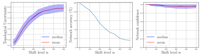
Figure 5: (Top row) A $0$ digit from the MNIST dataset exposed to increasing level of shift (pixel corruption). (Bottom row), (Left). The TU (with $0.1$ and $0.9$ quantiles) of corrupted inputs in the MNIST dataset with respect to the corruption level $n$. (middle) The accuracy of the network on these data (that is, the proportion of observations that are still correctly classified). (right) The confidence of the network in its predictions. Although the accuracy is dropping significantly, the network remains overall extremely confident in its predictions.

This last experimental subsection is dedicated to distribution shift. Distribution shifts share similar ideas with OOD-detection, in the sense that the network will be confronted to samples that are not following the training distribution. However, the difference lies in the fact that these new observations are shifted instances of observations that would be sampled with respect to the training distribution. In particular, shifted instances still have an underlying label that one may hope to recover. Formally, given a training distribution $\mathcal{X}$ and a parametric family of shifts $(s_{\gamma})_{\gamma}$ with the convention that $s_{0}=\mathrm{id}$, a shifted sample with level of shift $\gamma$ is a sample $s_{\gamma}(x_{1}),\dots,s_{\gamma}(x_{N})$, where $x_{1},\dots,x_{N}\sim\mathcal{X}$ with underlying labels $y_{1},\dots,y_{N}$. For instance, given an image, one can apply a corruption shift of parameter $\gamma=n\in\mathbb{N}$ where $s_{n}(x)$ consists of randomly switching $n$ pixels of the image $x$ ($x_{ij}\mapsto 1-x_{ij}$). See the top row of Figure 5 for an illustration.

Ideally, one would hope a trained network $F$ to be robust to shifts, that is $\operatorname*{arg\,max}(F(x))=\operatorname*{arg\,max}(F(s_{\gamma}(x)))$. However, since the map $x\mapsto s_{\gamma}(x)$ cannot be inverted in general, one cannot realistically expect robustness to hold for high levels of shift. Here, we illustrate how TU can be used as a way to monitor the presence of shifts that would lead to a dramatic diminution of the network accuracy in situations where the network confidence would be helpless.

For this, we train a network on MNIST and, following the methodology presented in Section 3, store the corresponding average persistence diagrams for the $10$ classes appearing in the training set. We then expose a batch of $1000$ observations from the test set containing $100$ instances of each class (that have thus not been seen by the network during the training phase) to the corruption shifts with various shift levels $n\in\{0,10,20,50,100,150,\dots,500\}$. For each shift level, we evaluate the distributions of TUs and confidences attributed by the network to each sample, along with the accuracy of the network over the batch. As illustrated in the second row of Figure 5, as the batch shifts, the TU increases and the accuracy drops. However, the network confidence remains very close to $1$, making this indicator unable to account for the shift. In practice, one can monitor a network by routinely evaluating the distribution of TUs of a new batch (e.g., daily recorded data). A sudden change in this 1D distribution is likely to reflect a shift in the distribution of observations that may itself lead to a drop in accuracy (or the apparition of OOD samples as illustrated in Subsection 4.2).

We end this subsection by stressing that the empirical relation we observe between the TU and the network accuracy cannot be guaranteed without further assumption on the law $(\mathcal{X},\mathcal{Y})$. It however occurs consistently in our experiments (see the appendix for complementary experiments involving different types of shift and network architectures). Studying the theoretical behavior of the TU and activation graphs in general will be the focus of further works.

5 Conclusion and perspectives

Monitoring trained neural networks deployed in practical applications is of major importance and is challenging when facing samples coming from a distribution that differs from the training one. While previous works focus on improving the behavior of the network confidence, in this article we propose to investigate the whole network instead of restricting to its final layer. By considering a network as a sequence of bipartite graphs on top of which we extract topological features, we introduce the Topological Uncertainty, a tool to compactly quantify if a new observation activates the network in the same way as training samples did. This notion can be adapted to a wide range of networks and is entirely independent from the way the network was trained. We illustrate numerically how it can be used to monitor networks and how it turns out to be a strong alternative to network confidence on these tasks. We will make our implementation publicly available.

We believe that this work will motivate further developments involving Topological Uncertainty, and more generally activation graphs, when it comes to understand and monitor neural networks. In particular, most techniques introduced in recent years to improve confidence-based descriptors may be declined to be used with Topological Uncertainty. These trails of research will be investigated in future work.

Appendix A Elements of Topological Data Analysis and theoretical considerations

A.1 Construction of persistence diagrams for activation graphs.

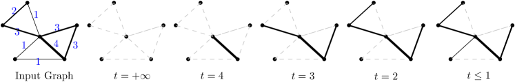
Figure 6: The super-level set filtration of a weighted graph, where we only draw edges that connect two connected components (not those creating loops). The filtration ends up with a Maximum Spanning Tree of the graph.

In this section, we provide a brief introduction to Topological Data Analysis (TDA) and refer to Edelsbrunner and Harer [2010]; Oudot [2015]; Chazal and Michel [2017] for a more complete description of this field.

Let $X$ be a topological space and $f\colon X\to\mathbb{R}$ be a real-valued continuous function. The sublevel set of parameter $t$ of $(X,f)$ is the set $\mathcal{F}_{t}:=\{x\in X\;:\;f(x)\leq t\}\subseteq X$. As $t$ increases from $-\infty$ to $+\infty$, one gets an increasing sequence (i.e., nested with respect to the inclusion) of topological spaces called the filtration of $X$ by $f$. Given such a filtration, persistent homology tracks the times $t$ of appearance and disappearance of topological features (such as connected components, loops, cavities, etc.). For instance, a new connected component may appear at time $t_{1}$ in the sublevel set $\mathcal{F}_{t_{1}}$, and may disappear—that is, it may get merged with an already present, other connected component—at time $t_{2}\geq t_{1}$. We say that this connected component persists over the interval $[t_{1},t_{2}]$ and we store the pairs $(t_{1},t_{2})$ as a point cloud in the Euclidean plane called the persistence diagram of the sublevel sets of $(X,f)$. Persistence diagrams of the superlevel sets are defined similarly. We refer to Figure 6 for an illustration.

Now, given a graph $G=(V,E)$ and a weight function $w\colon E\to\mathbb{R}$, we build a superlevel set persistence diagram as follows: at $t=+\infty$ (i.e., at the very beginning), we add all the nodes $V$. Then, we build a sequence of subgraphs $G_{t}=\{(V,E_{t})\}$ with $E_{t}=\{e\in E\,:\,w(e)\geq t\}$, that is, we add edges in decreasing order with respect to their weights. In this process, no new connected component can be created (we never add new vertices), and each new edge inserted at time $t$ either connects two previously independent components leading to a point with coordinates $(+\infty,t)$ in the persistence diagram, or creates a new loop in the graph. In our construction, we propose to only keep track of connected components ($0$-dimensional topological features). Since all points in the persistence diagram have $+\infty$ as first coordinate, we simply discard it and end up with a distribution of real numbers $t_{1}\geq\dots\geq t_{N}$, where $N=|V|-1$, which exactly corresponds to the weights of a maximum spanning tree built on top of $G$, see for instance [Doraiswamy et al., 2020, Proof of Lemma 2] for a proof.

Therefore, in our setting, we can compute the persistence diagram of an activation graph $G_{\ell}(x,F)$ connecting two layers, using the weight function $w\colon e\mapsto|W_{\ell}(i,j)x_{\ell}(i)|$, where $e$ is the edge connecting the $i$-th unit of the input layer to the $j$-th unit of the output layer.

A comparison with Neural persistence.

Given a bipartite graph, the construction we propose is exactly the one introduced in Rieck et al. [2019]. The difference between the two approaches is that loc. cit. works with the network weights $|W_{\ell}(i,j)|$ directly, obtaining one graph for each layer of the network $F$, while we use activation graphs $G_{\ell}(x,F)$ with weights $|W_{\ell}(i,j)x_{\ell}(i)|$, so that we obtain one graph per observation $x$ for each layer of the network. Then, both approaches compute a persistence diagram (MST) on top of their respective graphs. The second difference is that, in order to make use of their persistence diagrams in a quantitative way, Rieck et al. [2019] proposes to compute their total persistence, which is exactly the distance between a given diagram and the empty one (forcing to match all the points of the given diagram onto the diagonal $\Delta$). Taking advantage of the fact that our diagrams always have the same number of points (determined by the in- and out-layers sizes), we instead propose to compute distances to a reference diagram, namely the Fréchet mean of diagrams obtained on the training set. This allows us to compactly summarize information contained in the training set and use it to monitor the network behavior when facing new observations.

A.2 Metrics and Stability results.

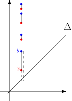
Figure 7: Two persistence diagrams whose points are distributed on the real line. Since we use $\|\cdot\|_{1}$ as a ground metric between diagram points, the distance between any two points $x$ and $y$ is always smaller than or equal to the sum of their distances to the diagonal. Therefore, an optimal partial matching between the two persistence diagrams can be obtained by simply matching points in increasing order (plain lines).

Diagram metrics in our setting.

Let $\Delta=\{(t,t)\in\mathbb{R}^{2}\}$ denote the diagonal of the Euclidean plane. Let $\mu,\nu$ be two diagrams with points $X:=\{x_{1},\dots,x_{n}\}\subseteq\mathbb{R}^{2}$ and $Y:=\{y_{1},\dots,y_{m}\}\subseteq\mathbb{R}^{2}$, respectively. Persistence diagrams are compared using optimal partial matching metrics. Namely, given a parameter $1\leq p\leq+\infty$, the $p$-th diagram metric is defined by

$$\mathbf{d}_{p}(\mu,\nu)=\left(\inf_{\gamma}\sum_{x\in X\cup\Delta}\|x-\gamma(x)\|^{p}_{1}\mathrm{d}x\right)^{1/p},$$ (7)

where $\gamma$ ranges over bijections between $X\cup\Delta$ and $Y\cup\Delta$. Intuitively, it means that one can either match points in $X$ to points in $Y$, or match points in $X$ (resp. in $Y$) to their orthogonal projections onto the diagonal $\Delta$. Among all the possible bijections, the optimal one is selected and used for computing the distance.

This combinatorial problem is computationally expensive to solve (a fortiori, so is the one of computing Fréchet means for this metric). Fortunately, in our setting, where diagrams are actually one-dimensional, that is, supported on the real line, and have the same number of points $N=d_{\ell}+d_{\ell+1}-1$, computing the optimal bijection becomes trivial. Indeed, one can observe first that, since we use $\|\cdot\|_{1}$ as our ground metric on the plane, it is never optimal to match a point $x\in X$ (resp. $y\in Y$) to the diagonal, since $\|x-y\|_{1}\leq\|x-s(x)\|_{1}+\|y-s(y)\|_{1}$, where $s$ denotes the orthogonal projection of a point onto the diagonal, see Figure 7. Since the persistence diagrams (that have to be compared) always have the same number of points in our setting, we can simply ignore the diagonal. In this way, we end up with an optimal matching problem between 1D measures. In that case, it is well-known that the optimal matching is given by matching points in increasing order, see for instance [Santambrogio, 2015, §2.1]. Thus, the distance $\mathrm{Dist}$ introduced in the article is equal to the distance $\mathbf{d}_{1}$ up to a normalization term $1/N$. This normalization is meant to prevent large layers from artificially increasing the distance between diagrams (and thus the Topological Uncertainty) and helps making distances over layers more comparable. The same normalization appears in Rieck et al. [2019].

Stability.

Let $G=(V,E)$ be a graph, and $w,w^{\prime}\colon E\to\mathbb{R}$ be two weight functions on its edges. In this context, the stability theorem (see for instance Chazal et al. [2016]) in TDA states that

$$\mathbf{d}_{\infty}(\mathrm{Dgm}(G,w),\mathrm{Dgm}(G,w^{\prime}))\leq\sup_{e\in E}|w(e)-w^{\prime}(e)|.$$ (8)

Now, let us consider a (sequential) neural network $F$ with $L$ layers and assume that all activations map $\sigma_{\ell}$ for $1\leq\ell\leq L-1$ are $1$-Lipschitz. We now introduce the notation

$$A_{\ell}=\sup_{i_{\ell},i_{\ell+1}}\sum_{i_{\ell}=1}^{d_{\ell}}|W_{\ell}(i_{\ell},i_{\ell+1})|.$$

Then, the map $x_{\ell}\mapsto\sigma_{\ell}(W_{\ell}x_{\ell}+b_{\ell})$ is an $A_{\ell}$-Lipschitz transformation (for the $\|\cdot\|_{\infty}$ norm). Indeed, one has:

$$\sup_{1\leq i_{\ell+1}\leq d_{\ell+1}}\bigg{\|}\sigma_{\ell}\left(\sum_{i_{\ell}=1}^{d_{\ell}}W_{\ell}(i_{\ell},i_{\ell+1})x_{\ell}(i_{\ell})+b_{\ell}(i_{\ell})\right)$$ (9)

$$-\sigma_{\ell}\left(\sum_{i_{\ell}=1}^{d_{\ell}}W_{\ell}(i_{\ell},i_{\ell+1})y_{\ell}(i_{\ell})+b_{\ell}(i_{\ell})\right)\bigg{\|}$$ (10)

$$\leq \sup_{1\leq i_{\ell+1}\leq d_{\ell+1}}\sum_{i_{\ell}=1}^{d_{\ell}}|W_{\ell}(i_{\ell},i_{\ell+1})||x_{\ell}(i_{\ell})-y_{\ell}(i_{\ell})|$$ (11)

$$\leq A_{\ell}\|x_{\ell}-y_{\ell}\|_{\infty}.$$ (12)

Therefore, the map $x\mapsto x_{\ell}$ is Lipschitz with Lipschitz constant $\mathcal{A}_{\ell}:=\prod_{\ell^{\prime}\leq\ell}A_{\ell^{\prime}}$. Now, using the stability theorem, we know that for $x,y$ two observations, one has

$$\mathbf{d}_{\infty}(D_{\ell}(x,F),D_{\ell}(y,F))\leq\mathcal{A}_{\ell}\|x-y\|_{\infty}.$$ (13)

Finally, observe that $\frac{1}{N}\mathbf{d}_{1}\leq\mathbf{d}_{\infty}$, so that the same result holds using the metric $\mathrm{Dist}$ introduced in the main paper.

We end this subsection by highlighting that, contrary to most applications of TDA, having a low Lipschitz constant in our stability result is not crucial as we actually want to be able to separate observations based on their Topological Uncertainties. Nevertheless, studying and proving results in this vein is of great importance in order to understand the theoretical properties of Topological Uncertainty, a project that we left for further work.

Appendix B Complementary experimental details and results

Implementation.

Our implementation relies on tensorflow 2 Abadi et al. [2016] for neural network training and on Gudhi Maria et al. [2014] for persistence diagrams (MST) computation. Note that instantiating the SimplexTree (representation of the activation of the graph in Gudhi) from the matrix $(|W_{\ell}(i,j)x_{\ell}(i)|)_{ij}$ is the limiting factor in terms of running time in our current implementation, taking up to $0.9$ second on a $784\times 512$ dense matrix for instance. Using a more suited framework to turn a matrix into a MST may drastically improve the computational efficiency of our approach. As a comparison, extracting a MST of a graph using Gudhi only takes about $0.03$ second.

B.1 Datasets.

Datasets description.

The MNIST and FMNIST datasets LeCun and Cortes [2010]; Xiao et al. [2017] both consist of training data and $10,000$ test data that are grey-scaled images of shape $28\times 28$), separated in $10$ classes, representing hand-written digits and fashion articles, respectively.

The CIFAR10 dataset Krizhevsky [2009] is a set of RGB images of shape $32\times 32\times 3$, separated in $10$ classes, representing natural images (airplanes, horses, etc.).

The SVHN dataset (Street View House Number) Netzer et al. [2011] is a dataset of RGB images of shape $32\times 32\times 3$, separated in $10$ classes, representing digits taken from natural images.

The DTD dataset (Describable Texture Dataset) Cimpoi et al. [2014] is a set of RGB images whose shape can vary between $300\times 300\times 3$ and $640\times 640\times 3$, separated in 47 classes.

Finally, Gaussian and Uniform refers to synthetic dataset of images of shape $32\times 32\times 3$ where pixels are sampled i.i.d following a normal distribution $\mathcal{N}(0.5,0.1)$ and a uniform distribution on $[0,1]$, respectively.

The MUTAG dataset is a small set of graphs (188 graphs) coming from chemestry, separated in $2$ classes. Graphs have on average $17.9$ vertices and and $19.8$ edges. They do not contain nodes or edges attributes and are undirected.

The COX2 dataset is a small set of graphs (467 graphs) coming from chemestry, separated in $2$ classes. Graphs have on average $41.2$ vertices and and $43.7$ edges. They do not contain nodes or edges attributes and are undirected.

Preprocessing.

All natural images datasets are rescaled to have coordinates in $[0,1]$ (from $[0,255]$). The coordinates of images belonging to the Gaussian dataset are thresholded to $[0,1]$. When feeding a network trained on CIFAR10 with smaller grey-scaled images (from MNIST and FMNIST), we pad the smaller images with zeros (by adding two columns (resp. rows) on the left and on the right of the image) and repeat the grey-scale matrix along the three channels. Conversely, we randomly sub-sample $32\times 32\times 3$ patches for images coming from the DTD dataset, as typically done in similar experiments.

The preprocessing of graphs datasets is slightly more subtle. In order to describe graphs as Euclidean vectors, we follow a procedure described in Carrière et al. [2020]. We compute the first $30$ eigenvalues of their normalized Laplacian (or pad with $0$s if there is less than $30$ eigenvalues). Additionally, we compute the quantile of the Heat Kernel Signature of the graphs with parameter $t=10$ as suggested in Carrière et al. [2020]. This processing was observed to be sufficient to reach fairly good accuracies on both MUTAG and COX2, namely $\sim 88$% on MUTAG and $\sim 78\%$ on COX2, about $2-3\%$ below the state-of-the-art results reported in [Carrière et al., 2020, Table 2].

B.2 Networks architectures and training.

Depending on the type of data and the dataset difficulty, we tried our approach on different architectures.

• For MUTAG and COX2, we used a simple network with one-hidden layer with 32 units and ReLU activation. The input and the hidden layer are followed by Batch normalization operations.

• For networks trained on MNIST and FMNIST, we used the reference architecture described at https://github.com/pytorch/examples/tree/master/mnist (although reproduced in tensorflow 2). When computing TU on top of this architecture, we only take the two final fully-connected layers into account (see the paragraph Remarks in the main paper).

• For networks trained on CIFAR-10, we used the architecture in https://www.tensorflow.org/tutorials/images/cnn.

All networks are trained using the ADAM optimizer Kingma and Ba [2015] (from tensorflow) with its defaults parameters, except for graph datasets where the learning rate is taken to be $0.01$.

B.3 Complementary experimental results.

We provide in this subsection some complementary experimental results and discussions that aim at putting some perspective on our work.

About trained network selection.

First, we stress that the results we obtain using either the TU or the confidence can probably be improved by a large margin: if the method was perfectly reliable, one would expect a $\sim+50\%$ increase between the accuracy obtained by a network with low TU (resp. high confidence) and the accuracy obtained by a network with high TU (resp. low confidence). Indeed, this would indicate that the score clearly separates networks that perfectly split the input dataset (leading to an accuracy of $\sim 100\%$) and those which classify all the points in a similar way (accuracy of $50\%$).

OOD detection: complementary illustrations.

Figure 8 shows the distribution of the TU for a network trained on the CIFAR-10 datasets (from which we store average persistence diagrams used to compute the TU) and a series of OOD datasets. Although the results are less conclusive that those obtained on graph datasets, the distribution of TUs on training data remains well concentrated around low values while being more spread for OOD datasets (with the exception of the DTD dataset, on which our approach indeed performs poorly), still allowing for a decent detection rate. Figure 9 provides a similar illustration for a network trained on MNIST using FMNIST as an OOD dataset. On this example, interestingly, the confidence baseline Hendrycks and Gimpel [2017] achieves a perfect FPR at 95% TPR of $0\%$ and an AUC of $64$, while our TU baseline achieves a FPR at 95% of $5\%$ (slightly worse than the confidence baseline) but an overall good AUC of $98$.

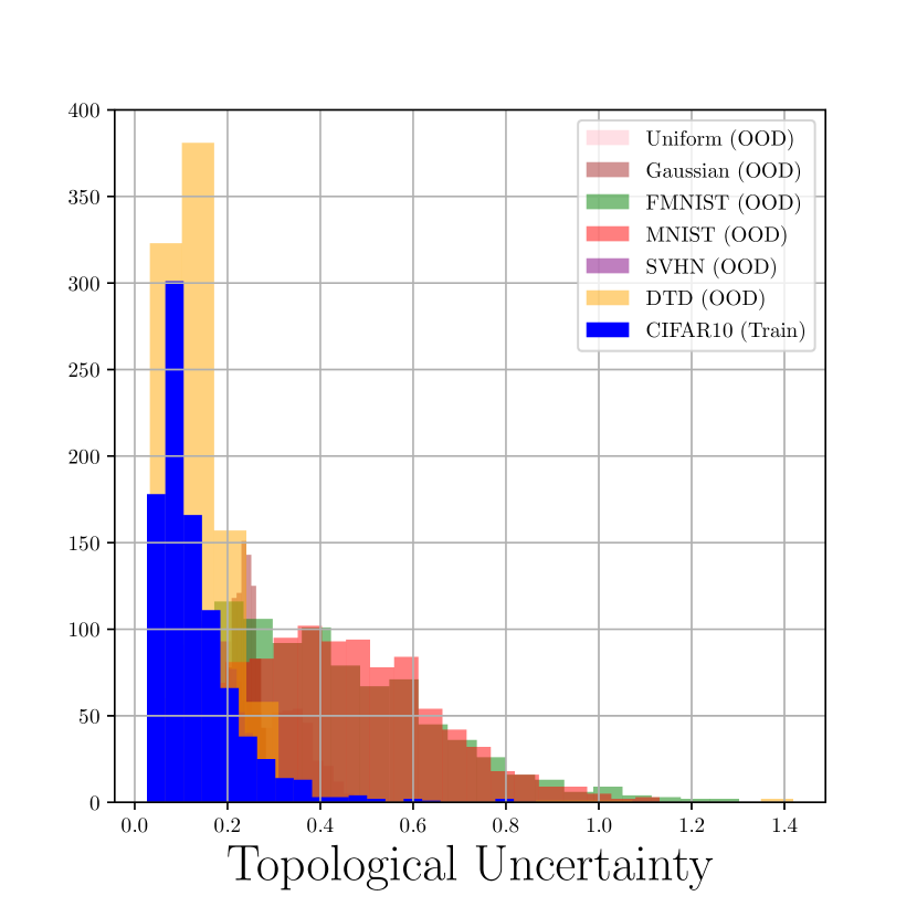
Figure 8: Distribution of TU for the CIFAR-10 dataset (training set) and OOD datasets.

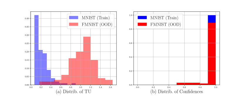
Figure 9: Distributions of TU and Confidence for a network trained on the MNIST dataset, using FMNIST as an OOD dataset.

Sensitivity to shift under Gaussian blur.

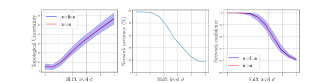
Figure 10: (Top row) A $0$ digit from the MNIST dataset exposed to increasing level of shift (Gaussian blur). (Bottom row), (Left). The TU (with $0.1$ and $0.9$ quantiles) of corrupted inputs in the MNIST dataset with respect to the corruption level $\sigma$. (middle) The accuracy of the network on these data (that is, the proportion of observations that are still correctly classified). (right) The confidence of the network in its predictions.

Figure 10 illustrates the behavior of TU, accuracy, and network confidence when data from the MNIST are exposed to Gaussian blur of variance $\sigma\in[0,5]$ (see the top row for an illustration). The increase in TU accounts for the shift in the distribution in a convincing way. Interestingly, on this example, the confidence reflects the shift (and the drop in accuracy) in a satisfactory way, contrary to what happens when using a corruption shift.

References

- Abadi et al. [2016] Martín Abadi, Paul Barham, Jianmin Chen, Zhifeng Chen, Andy Davis, Jeffrey Dean, Matthieu Devin, Sanjay Ghemawat, Geoffrey Irving, Michael Isard, et al. Tensorflow: A system for large-scale machine learning. In 12th USENIX symposium on operating systems design and implementation (OSDI 16), pages 265–283, 2016.
- Akhtar and Mian [2018] Naveed Akhtar and Ajmal Mian. Threat of adversarial attacks on deep learning in computer vision: A survey. IEEE Access, 6:14410–14430, 2018.
- Atzmon et al. [2019] Matan Atzmon, Niv Haim, Lior Yariv, Ofer Israelov, Haggai Maron, and Yaron Lipman. Controlling neural level sets. In NeurIPS, pages 2034–2043, 2019.
- Biggio and Roli [2018] Battista Biggio and Fabio Roli. Wild patterns: Ten years after the rise of adversarial machine learning. Pattern Recognition, 84:317–331, 2018.
- Carlsson and Gabrielsson [2020] Gunnar Carlsson and Rickard Brüel Gabrielsson. Topological approaches to deep learning. In Topological Data Analysis, pages 119–146. Springer, 2020.
- Carrière et al. [2020] Mathieu Carrière, Frédéric Chazal, Yuichi Ike, Théo Lacombe, Martin Royer, and Yuhei Umeda. Perslay: a neural network layer for persistence diagrams and new graph topological signatures. In AISTATS, pages 2786–2796. PMLR, 2020.
- Chazal and Michel [2017] Frédéric Chazal and Bertrand Michel. An introduction to topological data analysis: fundamental and practical aspects for data scientists. arXiv preprint arXiv:1710.04019, 2017.
- Chazal et al. [2016] Frédéric Chazal, Vin De Silva, Marc Glisse, and Steve Oudot. The structure and stability of persistence modules. Springer, 2016.
- Chen et al. [2020] Jiefeng Chen, Yixuan Li, Xi Wu, Yingyu Liang, and Somesh Jha. Robust out-of-distribution detection via informative outlier mining. arXiv preprint arXiv:2006.15207, 2020.
- Cimpoi et al. [2014] Mircea Cimpoi, Subhransu Maji, Iasonas Kokkinos, Sammy Mohamed, and Andrea Vedaldi. Describing textures in the wild. In Proceedings of the IEEE Conference on Computer Vision and Pattern Recognition, pages 3606–3613, 2014.
- DeVries and Taylor [2018] Terrance DeVries and Graham W Taylor. Learning confidence for out-of-distribution detection in neural networks. arXiv preprint arXiv:1802.04865, 2018.
- Doraiswamy et al. [2020] Harish Doraiswamy, Julien Tierny, Paulo JS Silva, Luis Gustavo Nonato, and Claudio Silva. Topomap: A 0-dimensional homology preserving projection of high-dimensional data. arXiv preprint arXiv:2009.01512, 2020.
- Edelsbrunner and Harer [2010] Herbert Edelsbrunner and John Harer. Computational topology: an introduction. American Mathematical Soc., 2010.
- Gebhart and Schrater [2017] Thomas Gebhart and Paul Schrater. Adversary detection in neural networks via persistent homology. arXiv preprint arXiv:1711.10056, 2017.
- Gebhart et al. [2019] Thomas Gebhart, Paul Schrater, and Alan Hylton. Characterizing the shape of activation space in deep neural networks. In 2019 18th IEEE ICMLA, pages 1537–1542. IEEE, 2019.
- Guo et al. [2017] Chuan Guo, Geoff Pleiss, Yu Sun, and Kilian Q Weinberger. On calibration of modern neural networks. In ICML, pages 1321–1330, 2017.
- Guss and Salakhutdinov [2018] William H Guss and Ruslan Salakhutdinov. On characterizing the capacity of neural networks using algebraic topology. arXiv preprint arXiv:1802.04443, 2018.
- Hein et al. [2019] Matthias Hein, Maksym Andriushchenko, and Julian Bitterwolf. Why relu networks yield high-confidence predictions far away from the training data and how to mitigate the problem. In Proceedings of the IEEE Conference on Computer Vision and Pattern Recognition, pages 41–50, 2019.
- Hendrycks and Dietterich [2019] Dan Hendrycks and Thomas Dietterich. Benchmarking neural network robustness to common corruptions and perturbations. arXiv preprint arXiv:1903.12261, 2019.
- Hendrycks and Gimpel [2017] Dan Hendrycks and Kevin Gimpel. A baseline for detecting misclassified and out-of-distribution examples in neural networks. ICLR, 2017.
- Hendrycks et al. [2019] Dan Hendrycks, Mantas Mazeika, and Thomas Dietterich. Deep anomaly detection with outlier exposure. ICLR, 2019.
- Kerber et al. [2017] Michael Kerber, Dmitriy Morozov, and Arnur Nigmetov. Geometry helps to compare persistence diagrams. Journal of Experimental Algorithmics (JEA), 22:1–20, 2017.
- Kingma and Ba [2015] Diederik P Kingma and Jimmy Ba. Adam: A method for stochastic optimization. ICLR, 2015.
- Krizhevsky [2009] Alex Krizhevsky. Learning multiple layers of features from tiny images. Technical report, 2009.
- Kumar et al. [2020] Abhishek Kumar, Benjamin Finley, Tristan Braud, Sasu Tarkoma, and Pan Hui. Marketplace for ai models. arXiv preprint arXiv:2003.01593, 2020.
- Lakshminarayanan et al. [2017] Balaji Lakshminarayanan, Alexander Pritzel, and Charles Blundell. Simple and scalable predictive uncertainty estimation using deep ensembles. NeurIPS, 30:6402–6413, 2017.
- LeCun and Cortes [2010] Yann LeCun and Corinna Cortes. MNIST handwritten digit database. 2010.
- Maria et al. [2014] Clément Maria, Jean-Daniel Boissonnat, Marc Glisse, and Mariette Yvinec. The gudhi library: Simplicial complexes and persistent homology. In International Congress on Mathematical Software, pages 167–174. Springer, 2014.
- Netzer et al. [2011] Yuval Netzer, Tao Wang, Adam Coates, Alessandro Bissacco, Bo Wu, and Andrew Y Ng. Reading digits in natural images with unsupervised feature learning. 2011.
- Nguyen et al. [2015] Anh Nguyen, Jason Yosinski, and Jeff Clune. Deep neural networks are easily fooled: High confidence predictions for unrecognizable images. In Proceedings of the IEEE conference on computer vision and pattern recognition, pages 427–436, 2015.
- Oudot [2015] Steve Oudot. Persistence theory: from quiver representations to data analysis. American Mathematical Society, 2015.
- Ovadia et al. [2019] Yaniv Ovadia, Emily Fertig, Jie Ren, Zachary Nado, David Sculley, Sebastian Nowozin, Joshua Dillon, Balaji Lakshminarayanan, and Jasper Snoek. Can you trust your model’s uncertainty? evaluating predictive uncertainty under dataset shift. In NeurIPS, pages 13991–14002, 2019.
- Ramamurthy et al. [2019] Karthikeyan Natesan Ramamurthy, Kush Varshney, and Krishnan Mody. Topological data analysis of decision boundaries with application to model selection. In ICML, pages 5351–5360. PMLR, 2019.
- Rieck et al. [2019] Bastian Alexander Rieck, Matteo Togninalli, Christian Bock, Michael Moor, Max Horn, Thomas Gumbsch, and Karsten Borgwardt. Neural persistence: A complexity measure for deep neural networks using algebraic topology. In ICLR. OpenReview, 2019.
- Santambrogio [2015] Filippo Santambrogio. Optimal transport for applied mathematicians. Birkäuser, NY, 55(58-63):94, 2015.
- Shorten and Khoshgoftaar [2019] Connor Shorten and Taghi M Khoshgoftaar. A survey on image data augmentation for deep learning. Journal of Big Data, 6(1):60, 2019.
- Torralba et al. [2008] Antonio Torralba, Rob Fergus, and William T Freeman. 80 million tiny images: A large data set for nonparametric object and scene recognition. IEEE transactions on pattern analysis and machine intelligence, 30(11):1958–1970, 2008.
- Turner et al. [2014] Katharine Turner, Yuriy Mileyko, Sayan Mukherjee, and John Harer. Fréchet means for distributions of persistence diagrams. Discrete & Computational Geometry, 52(1):44–70, 2014.
- Van Amersfoort et al. [2020] Joost Van Amersfoort, Lewis Smith, Yee Whye Teh, and Yarin Gal. Uncertainty estimation using a single deep deterministic neural network. In ICML, volume 119 of Proceedings of Machine Learning Research, pages 9690–9700. PMLR, 13–18 Jul 2020.
- Xiao et al. [2017] Han Xiao, Kashif Rasul, and Roland Vollgraf. Fashion-mnist: a novel image dataset for benchmarking machine learning algorithms. arXiv preprint arXiv:1708.07747, 2017.