On projection methods for functional time series forecasting

Abstract

Two nonparametric methods are presented for forecasting functional time series (FTS). The FTS we observe is a curve at a discrete-time point. We address both one-step-ahead forecasting and dynamic updating. Dynamic updating is a forward prediction of the unobserved segment of the most recent curve. Among the two proposed methods, the first one is a straightforward adaptation to FTS of the $k$-nearest neighbors methods for univariate time series forecasting. The second one is based on a selection of curves, termed the curve envelope, that aims to be representative in shape and magnitude of the most recent functional observation, either a whole curve or the observed part of a partially observed curve. In a similar fashion to $k$-nearest neighbors and other projection methods successfully used for time series forecasting, we “project” the $k$-nearest neighbors and the curves in the envelope for forecasting. In doing so, we keep track of the next period evolution of the curves. The methods are applied to simulated data, daily electricity demand, and NOx emissions and provide competitive results with and often superior to several benchmark predictions. The approach offers a model-free alternative to statistical methods based on FTS modeling to study the cyclic or seasonal behavior of many FTS.

1 Introduction

In the last few decades, technological advancements have simplified and decreased the cost of data collecting and storing processes. This new paradigm has made data scientific to confront not only big data sets but also complex data structures. Functional data analysis (FDA) arises naturally in this context to exploit the information recorded over a continuum such as time or space. The literature has experienced a prominent development of techniques and tools to take advantage of this kind of data. While the monographs of [60, 23, 38] provide complete picture of the methodological and theoretical contributions, recent advances in the field can be found in survey papers [18, 27, 79, 1].

This article addresses the problem of forecasting functional time series (FTS). These are time series $\{y_{k},k\in\mathbb{N}\}$ where each $y_{k}$ is a random function $t\rightarrow y_{k}(t)$, $t\in[a,b]$. We refer the reader to Hörmann and Kokoszka [28] for theory and examples of FTS. One-step-ahead forecasting is one of the most important problems in FTS analysis, and it has been addressed by diverse prominent literature [see, e.g., 11, 7, 34, 3, 30, 31, 2, 9, 59]. Also, forward prediction of a curve which is already being observed, termed dynamic updating by Shang and Hyndman [66], a topic of current interest [64, 67]. As many classical methods for time series forecasting, for example, those based on the ARIMA family models, the benchmark methods for FTS forecasting are based on fitting some statistical model of some approximated data generation. The most common is to fit ARIMA or VAR models to the Functional Principal Components Scores (FPC) of the functions, see FAR model [34, 9]. Klepsch and Klüppelberg [37] considered Functional Moving Average (FMA) and FARMA. [42] and [41] consider functional autoregressive fractionally integrated moving average (ARFIMA). Here we discuss an alternative model-free approach that addresses both one-step-ahead forecasting and dynamic updating in a unified way.

The literature of artificial intelligence and machine learning for time series forecasting has gained considerable prominence over the last decade [see, e.g., 51]. Besides the lack of an underlying model, many of these methods exhibit interesting features compared with classical statistical methods, including their ability to capture nonlinearities [53]. Among the most powerful machine learning technics used for time series forecasting, we must mention artificial neural networks [82] and $k$-nearest neighbors (KNN). The simplicity of implementing the algorithm and its high accuracy have popularized KNN. It has demonstrated to be a strong contender in forecasting competitions [52]. The method can be schematized as follows:

1. Consider $T$ observations, $x_{1},\dots,x_{T}$, from a time series and a prediction horizon $h$. Our goal is to forecast $p=(x_{T+1},\dots,x_{T+h})$, i.e. the time series $h$ periods ahead.

2. Consider all the possible observed $(E+h)$-tuples $(x_{i-(E-1)},\dots,x_{i},x_{i+1},\dots,x_{i+h})$. This means $E\leq i\leq T-h$.

3. Denote ${\mathbb{x}}_{i}=(x_{i-(E-1)},\dots,x_{i})$ and its projection $P({\mathbb{x}}_{i})=(x_{i+1},\dots,x_{i+h})$. Note that $p$ is the projection of ${\mathbb{x}}_{T}$.

4. Find the $k$-nearest neighbors to ${\mathbb{x}}_{T}$ from $\{{\mathbb{x}}_{i},E\leq i\leq T-h\}$.

5. Predict $p$ by a convex combination of the projections of the $k$-nearest neighbors.

In addition to the distance function used to find the nearest neighbors and the convex combination used for predicting, KNN involves setting the sometimes called embedding dimension $E$ and the number of neighbors denoted by $k$. The simplex projection [71] and the S-map projection [70] are methods related to KNN that provide skillful forecasts, free of $k$.

Moreover, these model-free methods have outperformed any forecast based on models [58]. Surprisingly, functional versions have not been developed for FTS. In contrast, in the context of FDA, the KNN method has been explored and theoretically supported towards regression problems [12, 10, 40, 43] or functional classification problems [13, 29]. Biau et al. [10] introduces asymptotic results when the response variable has a finite dimension. Kara et al. [36] provides asymptotic results that, exceptionally, allows for an automatic choice data-driven of the number of neighbors for several operators, among them functional regression with a scalar response. Lian [43] proves the consistency of the KNN regression estimate when both dependent and independent variables are functions. Recently, [22] use the nearest neighbours method for bandwidth selection on a problem of scalar-on-function local linear regression. Remarkably, [83] addresses the problem of forecasting final prices of auctions via functional KNN. Roughly, their forecasting is based on the $k$-nearest price curves to the item being predicted and their corresponding final prices. We consider dynamic updating in line with these authors. For example, if we predict afternoon electricity demand, we use afternoon data from days with morning data near to the morning of the day being predicted. For one-step-ahead forecasting, we mimic the projection procedure inherent to KNN. For example, for tomorrow’s forecasting electricity demand, we consider next-day demands of daily curves near to today. Moreover, we take ideas of [71], and we do not only consider the nearest daily curves but those that surround the most recent data from above and below, when this is possible, to select a neighbor that is representative of its shape and its magnitude. This is the key to produce coherent band predictions, in which the observed part of the day being predicted is inside the band delimited by the curves that we are using for predicting. Whereas the curve to predict may be entirely outside of the band delimited by its $k$-nearest curves. In this vein, we combine two concepts, nearness and centrality, commonly termed depth in the functional context.

Functional depth [56, 25] has received a great deal of attention since it was introduced by Fraiman and Muniz [24]. It has been used for several applications; including classification [46, 19, 16, 29, 17], outlier detection [21, 35, 8, 55, 54], populations comparison [47, 48, 74], and clustering [68, 75]. Functional versions of boxplots and other graphical tools based on different depths have also been proposed for visualizing curves to discover features from a sample that might not be apparent using other methods [32, 72, 62, 20]. However, up to our knowledge, the concept of depth has not been used for forecasting.

Here we introduce a depth-based projection method for forecasting that constitutes a contribution to the literature of nonparametric FDA, an area popularized by [23] and that it is actively growing, see the review by Ling and Vieu [44]. Also, we consider an adaptation to FTS of the KNN briefly schematized above and we follow ideas from [36] to make it automatic. We also consider several benchmark methods in the field for comparisons. For that, we use daily functions of electricity demand and nitrogen monoxide (NOx) emissions. Both are FTS that have already been considered by the literature. Also, both exhibit a strong calendar-effect [78], making them appropriate to illustrate the excellent performance of the method discussed here. As we discuss below, the projection methods have been intended to forecast FTS with seasonal or cyclical patterns. Through a simulation study, we investigate the impact on forecast accuracy from the departure of stationarity. We remark that, although we do not assume any stationarity of first or second order, we do not consider applications to FTS with a significant trend. Specifically, we suppose the curves of the FTS fluctuate in a finite band.

This paper is organized as follows. Section 2 describes the projection methods considered here. Section 3 provides results of comparing the proposed methods with benchmark methods. Section 4 concludes with a general discussion.

2 Projection methods for forecasting

Let $\{y_{i},i\in\mathbb{N}\}$ be a FTS [28]. Here, we assume that each $y_{i}$ is a univariate random function and, without loss of generality, we suppose that its domain is $[0,1]$.

2.1 Basic notions

We consider two scenarios of prediction:

• One-step-ahead forecasting; when we have observed $y_{1},...,y_{n}$ on $[0,1]$, and we want to predict $\{y_{n+1}(t):t\in[0,1]\}$.

• Dynamic updating; when we have observed $y_{1},...,y_{n-1}$ on $[0,1]$ and $y_{n}(t)$ on $[0,q]$, for a given $0\ll q<1$, and we want to predict $\{y_{n}(t):t\in(q,1]\}$.

In both scenarios, we refer to the most recently observed functional datum, either $\{y_{n}(t):t\in[0,1]\}$ or $\{y_{n}(t):t\in[0,q]\}$, as the focal curve. The latter will be denoted by $f$ and its observation domain by $D_{f}$, regardless of whether it is $[0,1]$ or $[0,q]$. For each $i$, $1\leq i\leq n-1$, we consider the restriction of $y_{i}$ to $D_{f}$, this is the curve with graph equal to $\{(t,y_{i}(t)):t\in D_{f}\}$. We denote this restriction by $y_{i|f}$ and we refer to ${\cal Y}_{n}=\{y_{1|f},\dots y_{n-1|f}\}$ as the past-focal-curves sample. Note that in one-step-ahead forecasting $y_{i|f}\equiv y_{i}$ .

Denote by $p$ the curve or curve segment to predict, this is $\{y_{n+1}(t):t\in[0,1]\}$ or $\{y_{n}(t):t\in(q,1]\}$. The domain of $p$, either $[0,1]$ or $(q,1]$, is denoted by $D_{p}$. Then, for each $y_{i|f}\in{\cal Y}_{n}$, we consider the projection

$${\cal P}y_{i|f}=\begin{cases}\{y_{i+1}(t),t\in[0,1]\},&\mbox{in one-step-ahead forecasting.}\\ \{y_{i}(t),t\in(q,1]\},&\mbox{in dynamic updating.}\\ \end{cases}$$

Note that ${\cal P}f=p$ and that, although not explored it in this article, $h$-step-ahead projection could be achieved by ${\cal P}y_{i|f}=\{y_{i+h}(t),t\in[0,1]\}$.

Many FTS regularly repeat dependency patterns between past focal curves and their projections. The change in shape and magnitude of the curves over time of some FTS can be visualized from the rainbow plots of Hyndman and Shang [32] and other related plots [65].

In dynamic updating, we observe that $y_{i|f}$ and ${\cal P}y_{i|f}$ are a partition of $y_{i}$ in two curve segments. The dependence patterns between past focal curves and their projections can be observed from groups of curves with similar colors in the rainbow plots already mentioned. Similar curves may be distant in time due to seasons and cycles, making specific patterns be repeated over time. It is not necessarily an easy task to visualize dependency patterns between focal curves and their projections; it depends on the complexity of the FTS and the curves’ shapes, and the number of curves involved. Nonetheless, the cyclic nature of many FTS suggests that there may be statistical regularity between the morphology of focal curves and the morphology of their projections. The core idea of the methods discussed here is based on the existence of this kind of regularity. Thus, if $f$ is surrounded by past focal curves that capture both its shape and magnitude, we could predict $p$ from these past focal curves’ projections. Of course, when the FTS has a strong global trend, the future values are always out of the historical data magnitude. Therefore, the projection methods discussed here are not suitable without detrending in such cases.

2.2 The focal-curve envelope

The straightforward approach for surrounding $f$ with past focal curves is by using KNN. However, as we already commented, $f$ does not have to be necessarily centred in the band delimited by its $k$-nearest curves. Even $f$ may be completely outside of this band. To produce bands where $f$ is central, which is natural for band estimation, we use the concept of functional depth. In particular, we use the modified band depth of López-Pintado and Romo [47] with bands formed by two curves. This is a widely used depth measure that allows a million curves to be ranked in only tenths of seconds [73] making our algorithm efficient even for large data sets. Strictly speaking, for any $\mathcal{J}\subset{\cal Y}_{n}$ with $|\mathcal{J}|\geq 2$ and $y\in\mathcal{J}\cup\{f\}$, we consider

$$D(y,\mathcal{J})=\frac{1}{2}{|\mathcal{J}|+1\choose 2}^{-1}\sum_{x,z\in\mathcal{J}\cup\{f\}}\lambda\left(\left\{t\in D_{f}:\min(x(t),z(t))\leq y(t)\leq\max(x(t),z(t))\right\}\right),$$

$\lambda(\{t\in D_{f}:A(t)\})$ being the proportion of time that $A(t)$ is true on $D_{f}$. The larger $D(y,{\cal J})$, the deeper will be $y$ in ${\cal J}\cup\{f\}$. Denote by ${\cal J}_{k}$ the $k$ deepest curves of ${\cal J}$. We remark that $f\notin{\cal J}_{k}$ although $f$ may be the deepest curve of ${\cal J}\cup\{f\}$.

In line with Sun and Genton [72], who consider central regions based on the modified band depth for visualizing the spread of the deepest curves, we consider the Focal Central Region (FCR) delimited by ${\cal J}_{k}$. This is the region

$$R({\cal J}_{k})=\left\{(t,y(t)):t\in D_{f},\min_{x\in{\cal J}_{k}}x(t)\leq y(t)\leq\max_{x\in{\cal J}_{k}}x(t)\right\}.$$

So that $R({\cal J}_{k})$ can capture the shape and magnitude of $f$, $R({\cal J}_{k})$ must be roughly centered at $f$ and its mean width should be small. Having these objectives in mind, we look for a set ${\cal J}$ of past focal curves, as large as possible in order of not restricting the range of $k$, such that:

1. $f$ is deep in ${\cal J}\cup\{f\}$, the deepest if possible.

2. $f$ is enveloped by ${\cal J}$ as much as possible. Here, we say $f$ is more enveloped by ${\cal J}$ than by ${\cal J}^{\prime}$ if and only if

   $$\lambda\left(\left\{t:\min_{y\in{\cal J}}y(t)\leq f(t)\leq\max_{y\in{\cal J}}y(t)\right\}\right)>\lambda\left(\left\{t:\min_{y\in{\cal J}^{\prime}}y(t)\leq f(t)\leq\max_{y\in{\cal J}^{\prime}}y(t)\right\}\right).$$

3. $f$ is surrounded by near curves of ${\cal J}$, as many as possible.

Algorithm 1 provides a set of past focal curves with the three features above that we call the focal-curve envelope and denote by ${\cal J}$ from now on. In a nutshell, the algorithm iteratively selects as many past curves as possible. From the nearest to the farthest to $f$, we obtain an envelope of $f$ with an increasing depth.

Algorithm 1 Input: ${\cal Y}_{n},f$. Output: $\mathcal{J}$

Initialize ${\cal Y}={\cal Y}_{n}$, ${\cal J}=\emptyset$, $D(f,{\cal J})=0$

while  size of ${\cal Y}\geq 2$  do

    Let $y^{\prime}$ be the nearest curve to $f$ from ${\cal Y}$ and ${\cal N}=\{y^{\prime}\}$

    for  $y\in{\cal Y}\setminus\{y^{\prime}\}$, from the nearest curve to the farthest from $f$, do

         if $f$ is more enveloped by ${\cal N}\cup\{y\}$ than by ${\cal N}$ then

             ${\cal N}={\cal N}\cup\{y\}$

         end if

    end for

    if $D(f,{\cal J}\cup{\cal N})\geq D(f,{\cal J})$ then

         ${\cal J}={\cal J}\cup{\cal N}$

    end if

    ${\cal Y}={\cal Y}\setminus{\cal N}$

end while

As an illustration of how Algorithm 1 works, see top panels of Figure 1, where 100 curves from a simulated FTS are considered. The left panels show the twelve curves selected on the first iteration of Algorithm 1 (top panel) and the 12-nearest neighbors (bottom panel). For measuring nearness, hereafter, we use $L_{2}$ distance. Besides this is the most widely used distance in the KNN context, we base our choice by looking for a small mean squared error on the prediction method discussed in Subsection 2.3. We emphasize the intervals where the nearest curves do not envelope the focal curve. Right panels show the band delimited by the focal-curve envelope obtained after five iterations and formed by forty-six curves and the corresponding band from the 46-nearest curves. As a general rule, Algorithm 1 selects near curves that are enveloping the focal until it is the deepest one. In contrast, nearest neighbors neither necessarily envelope the focal curve nor make it the deepest one.

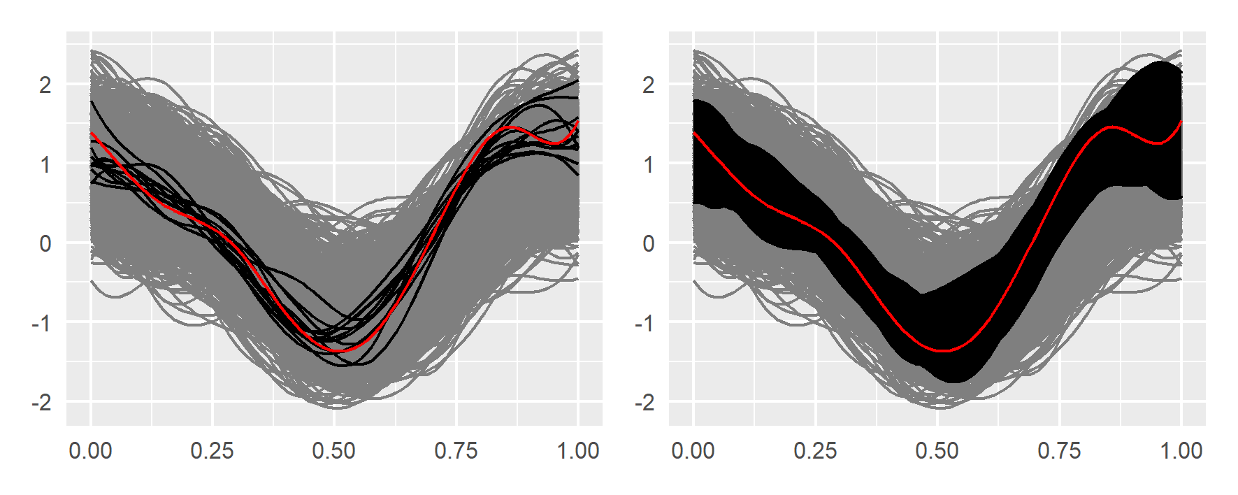
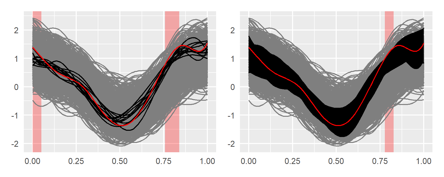
Fig. 1: Top panels: focal curves (in red), the twelve curves selected on the first iteration of Algorithm 1 (left panel) and band delimited by the focal-curve envelope from the 46 curves selected by the algorithm (right panel). Bottoms panels: The 12-nearest curves and the band delimited by the 46-nearest curves. The intervals where the nearest curves do not envelope the focal are shaded in red. Algorithm 1 selects near curves that envelope the focal until making it been the deepest one. The nearest curves do not necessarily envelope the focal curve nor making it been the deepest one.

2.3 Prediction

We make predictions by projecting the $k$-nearest curves to the focal and projecting the curves that belong to the focal-curve envelope. We compute weighted means of these projections for punctual prediction, assigning more weights to the curves closer to the focal. Following the literature on KNN [52, 36], and simplex projections or S-map [58], we consider two types of weights: On one hand, weights inversely proportional to the square distance to the focal, which we identify in the sequel by $1/d$ weights. On the other hand, exponential weights. Specifically, let $f_{1},\dots,f_{k}$ be the $k$-nearest curves to $f$, $d_{i}=\lVert f_{i}-f\rVert^{2}$, and more general $d_{y}=\lVert y-f\rVert^{2}$, let ${\cal J}$ be the focal-curve envelope of $f$ and $\theta>0$, what we do is to consider the following estimators of $p={\cal P}f$:

• functional KNN projections (fKNN) with $1/d$ and exponential weights

  $$\hat{p}_{k}=\frac{\sum_{i=1}^{k}\frac{1}{d_{i}}\ {\cal P}f_{i}}{\sum_{i=1}^{k}\frac{1}{d_{i}}},\ \ \mbox{and}\ \ \hat{p}_{k,\theta}=\frac{\sum_{i=1}^{k}e^{-\theta d_{i}/d_{1}}{\cal P}y}{\sum_{i=1}^{k}e^{-\theta d_{i}/d_{1}}}$$ (1)

• Envelope projections (EP) with $1/d$ and exponential weights

  $$\hat{p}=\frac{\sum_{y\in{\cal J}}\frac{1}{d_{i}}\ {\cal P}f_{i}}{\sum_{y\in{\cal J}}\frac{1}{d_{i}}},\ \ \mbox{and}\ \ \hat{p}_{\theta}=\frac{\sum_{y\in{\cal J}}e^{-\theta d_{y}/d_{1}}{\cal P}y}{\sum_{y\in{\cal J}}e^{-\theta d_{y}/d_{1}}}$$ (2)

For fixed $\theta$, $k$ in (1) will be chosen by minimizing the prediction Mean Square Error (MSE) on a rolling forecasting origin procedure, as it is customary in the literature of KNN for time series. We denote by $k^{*}$ the value that minimizes the MSE. Similarly, we can select $\theta$ in (2). Let $\theta^{*}$ be the resulting value of minimizing MSE by rolling origin. We discard selection of optimal pairs $(\theta,k)$ for $\hat{p}_{k,\theta}$ in (1) by a high computational cost involved in this two-dimensional optimization problem. To compare the methods, on one hand we compute $\hat{p}_{k}^{*}$ and $\hat{p}$. On the other hand, we fix $\theta=1$ and compute $\hat{p}_{k^{*},\theta=1}$ and $\hat{p}_{\theta=1}$. In addition, we compute $\hat{p}_{\theta^{*}}$.

For band prediction, we consider the region delimited by the projections of the $k$ deepest curves of ${\cal J}$. This is the band

$${\cal P}R({\cal J}_{k})=\left\{(t,y(t)):t\in D_{p},\min_{x\in{\cal J}_{k}}{\cal P}x(t)\leq y(t)\leq\max_{x\in{\cal J}_{k}}{\cal P}x(t)\right\}.$$

This band prediction corresponds to a central functional region such as those defined by [72]. As with the fKNN projections, $k$ is chosen by minimizing a rolling forecasting origin procedure’s cost function. For that, we consider the Winkler score. This is a measure that penalizes both bandwidth and non-coverage for a given $\alpha\in(0,1)$, penalizing even more heavily when observations are remarkably outside the band the confidence levels are higher [80, 26]. Thus, for a given $(1-\alpha)$ mean coverage, i.e., the proportion of time that $p$ is in the band, $k$ is chosen by minimizing the score. Mimicking this procedure, we also consider the region delimited by the projection of the $k$ nearest curves for band prediction based on fKNN.

Figure 2 shows an example of point and band prediction based on 1000 curves from a simulated FTS corresponding to the model discussed in Section 3.1 with $\mu=0$. Both one-step-ahead forecasting and dynamic updating provided by EP with $\hat{p}_{\theta}$ are illustrated.

Fig. 2: 1000 curves from a simulated FTS (grey). Focal curve $f$ in solid red, curve to predict $p$ in dashed red, point prediction $\hat{p}_{1}$ in blue and prediction band ${\cal P}R({\cal J}_{10})$ in black. Left panel: One-step-ahead prediction. Right panel: Dynamic updating from $0.5$ to $1$.

3 Results

For one-period-ahead forecasting, we compare fKNN and EP estimators with benchmark predictions for stationary FTS. In particular, we implement a variant of the method proposed by Hyndman and Ullah [34] and Hyndman and Shang [31], who suggest functional prediction based on modeling the functional principal component scores as independent time series. Following Aue et al. [9], we will consider the first $d$ functional scores as a $d$-variate time series since the score vectors could have non-diagonal autocorrelations. The number of scores $d$ is chosen as the smallest integer such that the first $d$ principal components explain at least 80% of the variance of the data. Then, we fit a $d$-dimensional autoregressive model [50] to the scores’ time series. This method is termed FPCF. For validating FPCF as a benchmark method, we repeated the simulation study conducted by Aue et al. [9] and obtained competitive results with the best of their methods (see Appendix 5.1).

For dynamic updating, we compare fKNN, and EP with the method of [39] for predicting partially observed functional data. We also tested the well-known method of Yao et al. [81] but Kraus [39] achieved better results in our experiments. When the FTS is constructed by slicing a periodic univariate time series, we also consider the Block-Moving (BM) approach by Shang and Hyndman [66]. The BM approach is designed to re-arrange the time series so that all the FTS are ultimately observed and, then, to apply FPCF is possible. The literature devoted to dynamic updating has successfully proposed methodologies based on ordinary least squares (OLS) regression, ridge regression (RR), penalized least squares (PLS) regression, or functional linear regression [66, 64, 67]. However, we do not compare with them because we deal with large data sets where these methods might be computationally inefficient. In other circumstances, they certainly are the benchmark of the field.

Finally, to understand the scale of how superior a method is with respect to the other, we also report about the two most basic estimators. They are the historical mean and the naive prediction. This is just the most recent observed datum corresponding to the prediction range. In our notation, the naive predictor of ${\cal P}y_{n}$ is ${\cal P}y_{n-1}$.

The implementation of the Envelope Projection method is available at https://github.com/aefdz/nnFTS. The benchmark methods for Functional Time Series are available in the ftsa R package by Hyndman and Shang [33]. Finally, the method for estimating partially observed data was implemented by [39] with the code available from https://www.davidkraus.net/?page_id=349.

3.1 Stationary FTS with random shocks

To simulate FTS with the features discussed at the end of Section 2.1, we consider slices of a scalar process with complex periodic rhythm that artificially corrupt with shocks. This process is denoted $Y_{\mu}$, being $\mu\in[0,1)$ the expected proportion of affected periods. The process is the sum of three independent components corresponding to:

1. A noise $\{X(t):t\geq 0\}$, modeled by a zero-mean stationary Gaussian process.

2. A random periodic function $f:[0,+\infty)\rightarrow\mathbb{R}$.

3. A random shock process $\{S_{\mu}(t):t\geq 0\}$ that occasionally affects two contiguous periods of $f$. For $\mu=0$, $S_{\mu}=0$.

See Appendix 5.2 for more details about these processes. Thus $Y_{\mu}=X+f+S_{\mu}$ and the considered FTS is $y_{i}(t)=Y_{\mu}(t+i-1)$, $0\leq t\leq 1$, $i\in\mathbb{N}$. If $\mu=0$, there are no shocks and the corresponding FTS is stationary. With increasing $\mu$, we explore different non-stationary regimes. Figure 3 shows two random trajectories of $Y_{0.2}$ and their respective FTS.

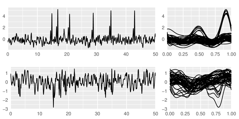
Fig. 3: Two random trajectories of $Y_{0.2}$ (left panel) and their corresponding FTS (right panel).

We performed 300 realizations of $Y_{\mu}$, 100 for each level of contamination considered. They were $\mu=0.0,0.2$ and $0.4$. For each realization, we considered $1000$ periods and, from the corresponding $1000$ slices, the exercise of one-step-ahead prediction and dynamic updating on the last $100$ slices. For dynamic updating, we chose $q=0.5$, corresponding to half slice. The resulting MSEs are shown in Table 1. In summary, we found the proposed methods were superior to the benchmark method. They were even better at higher contamination levels, and fKNN is often superior to EP.

Table 1: Mean Squared Errors for one-step-ahead forecasting and dynamic updating from a stationary FTS ($\mu=0$) contaminated with random shocks at two levels of contamination ($\mu=0.2$ and $\mu=0.4$). The observed minimum MSE among the considered methods is remarked in bold.

One-step-ahead prediction
			fKNN			EP
	Average	Naive	$\hat{p}_{k^{*}}$	$\hat{p}_{k^{*},\theta=1}$		$\hat{p}$	$\hat{p}_{\theta=1}$	$\hat{p}_{\theta^{*}}$	FPCF
$\mu=0.0$	0.192	0.385	0.1880	0.1879		0.192	0.199	0.192	0.190
$\mu=0.2$	2.465	5.380	1.5288	1.5153		1.646	1.679	1.594	1.662
$\mu=0.4$	4.513	11.35	2.5893	2.5974		2.912	2.832	2.744	2.767

Dynamic Updating
			fKNN			EPU
	Average	Naive	$\hat{p}_{k^{*}}$	$\hat{p}_{k^{*},\theta=1}$		$\hat{p}$	$\hat{p}_{\theta=1}$	$\hat{p}_{\theta^{*}}$	BM	Kraus
$\mu=0.0$	0.192	0.382	0.1582	0.1582		0.160	0.172	0.157	0.182	0.166
$\mu=0.2$	2.527	5.520	1.2109	1.1920		1.669	1.421	1.239	2.173	1.599
$\mu=0.4$	4.783	12.126	1.4078	1.3805		2.278	1.640	1.418	3.756	2.750

3.2 Spanish electricity demand

Functional methods for electricity demand forecasting have been widely used [77, 6, 57, 14, 63, 4, 5, 76, 59]. These methods often consider particular features of the data, such as weekly seasonality, the effect of holidays, and outliers’ presence. Thus, researchers process weekdays separately from Saturdays and Sundays and apply methods for replacing outliers. In addition to this, Raña et al. [59] use additional data from functional exogenous covariates in their Functional Additive Models (FAM) for next-day forecasting. Certainly, they provide the benchmark predictions in functional Spanish electricity demand forecasting.

We consider the challenge of predicting the daily curves of a whole year (2018) without considering any specific peculiarity of the electricity demand by using raw data. For dynamic updating, we considered the practical case of half-day ahead prediction. Our study is based on electricity demand at every 10-minute interval, from January 1, 2014, to December 31, 2018. The data set is available at http://www.ree.es/es/. Following Raña et al. [59], we compute the mean absolute percentage error (MAPE) in addition to the MSE. Viewing the weekly seasonality of electricity demand and the naive prediction corresponding to yesterday for predicting today, we also consider the naive prediction corresponding to the same day one week ago, identified below as seasonal naive (Naive^′ in the tables). The results are shown in Table 2.

Table 2: Forecasting accuracy for daily electricity demand during 2018. The performance is measure by MSE, MSE/MSE_min, being the MSE divided by the minimum MSE among the different methods and MAPE. The minimum value of each row is remarked in bold.

One-step-ahead prediction
				fKNN			EP
	Average	Naive	Naive’	$\hat{p}_{k^{*}}$	$\hat{p}_{k^{*},\theta=1}$		$\hat{p}$	$\hat{p}_{\theta=1}$	$\hat{p}_{\theta^{*}}$	FPCF
MSE	10139732	8011267	4448292	1537719	1530080		2144232	1440256	1416428	5771944
$\frac{\text{MSE}}{\text{MSE}_{\min}}$	7.158	5.655	3.140	1.086	1.080		1.514	1.017	1.000	4.075
MAPE	8.857	6.383	4.647	2.57953	2.59538		3.495	2.666	2.542	6.583

Dynamic Updating
				fKNN			EP
	Average	Naive	Naive’	$\hat{p}_{k^{*}}$	$\hat{p}_{k^{*},\theta=1}$		$\hat{p}$	$\hat{p}_{\theta=1}$	$\hat{p}_{\theta^{*}}$	BM	KRAUS
MSE	11545143	7805649	5245784	433620	426642		534009	414877	413508	2823846	512749.9
$\frac{\text{MSE}}{\text{MSE}_{\min}}$	27.92	18.877	12.687	1.049	1.032		1.291	1.003	1.000	6.829	1.240
MAPE	9.061	6.183	5.035	1.55566	1.55052		1.79564	1.54113	1.53637	4.43493	1.7558

From this table, we remark that FPCF is slightly inferior to the naive method and significantly inferior to seasonal naive. However, the projection methods were superior to the benchmark competitors for both one-step-ahead forecasting and dynamic updating, and EP slightly superior to fKNN.

Although they are different studies, MAPE of Raña et al. [59] (in the last four rows of the last column of their Table 1) might reference the expected magnitude of the forecasting performance. The naive method in both studies produces the same MAPE (6.383 vs. 6.39). However, we remark that MAPE computed by Raña et al. [59] corresponds to 2012 prediction instead of 2018, using demand each hour, instead of every 10 minutes, and therefore conclusions might be taken with caution. From this extrapolation, FPCF in Table 2 seems to be by far inferior to FAM. This points out the convenience of removing outliers and taking into account the data’s weekly seasonality to improve predictions as suggested by Raña et al. [59]. Finally, MAPE of fKNN and EP turned out to be by far smaller than those of FAM, despite being based on data without preprocessed, without splitting the data into Weekdays, Saturdays, and Sundays, and without covariates.

Notably, Raña et al. [59] also reports coverage and mean Winkler scores of prediction bands, providing an approximate order of magnitude of the results to compare them with the prediction bands based on projection methods introduced at the end of Subsection 2.3. Table 3 displays the scores resulting from projection methods for $\alpha=0.05,0.10$ and $0.20$. The first noteworthy result is that the mean coverages obtained are often above $(1-\alpha)$. Second, the mean Winkler scores are often smaller than that those previously reported.

Table 3: Coverage and mean Winkler score of prediction bands for electricity demand and NOx emissions.

		Electricity Demand						NoX Emission
		One-day-ahead			Dynamic Updating			One-day-ahead			Dynamic Updating
$\alpha$		EPF	fKNN		EPU	fKNN		EPF	fKNN		EPU	fKNN
$0.05$	Coverage	0.96	0.96		0.96	0.93		0.94	0.94		0.96	0.98
	(width)	6340.22	5581.59		3909.38	6871.60		88.64	81.07		99.56	95.59
	Winkler	7245.76	6200.67		4391.11	10326.45		103.94	94.95		108.16	97.85
$0.10$	Coverage	0.93	0.92		0.92	0.87		0.89	0.89		0.89	0.95
	(width)	5272.801	4477.16		3126.253	5881.41		71.16	68.91		60.41	79.47
	Winkler	6005.07	5097.22		3672.03	9969.236		87.23	84.90		71.70	83.81
$0.20$	Coverage	0.83	0.84		0.82	0.80		0.80	0.79		0.80	0.87
	(width)	4228.828	3355.45		2457.981	4794.38		56.93	54.54		47.43	64.04
	Winkler	5390.77	4185.80		3162.14	8344.702		75.13	75.06		60.34	71.79

Also, we want to remark that the projection methods take into account the weekly and yearly periodicity of the data without any prior information. For illustrating this, we plot the frequency distribution of the number of days between predicted days and days used in the EP prediction in Figure 4. The exponential weights properly averaged and scaled are also plotted in the same figure. This figure reveals the most relevant past information to forecast one-period-ahead and the electricity demand’s seasonal structure. In particular, we observe that the most recent day contributes the most to the point forecast, followed by the same weekday but one week before (highest bars at the bottom panel). This weekly contribution vanishes until we approach the values of one year ago (highest bars at the top panel). For example, if we aim to forecast the demand for a given Wednesday, then the envelope would consider data from the last Tuesday, past Wednesdays, and same calendar days of other years in the same season, in order of importance.

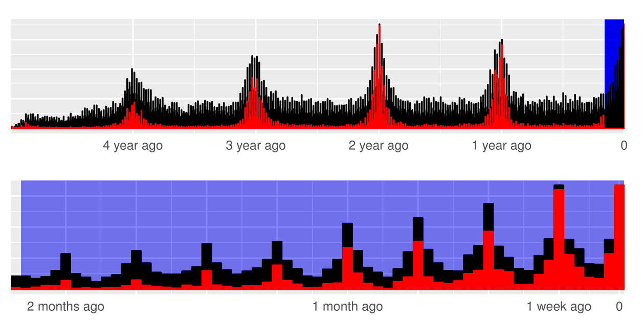
Fig. 4: Black bars: frequency distribution of the number of days between predicted day and the ones used in the EP prediction. Red bars: the normalized average of exponential weights used in the EP prediction. Bottom panel: zoom of the blue shaded area in the top panel.

3.3 NOx emissions in Madrid city center

Air quality is nowadays in the spotlight due to its impact on human health [45]. Many cities gather almost continuous data of different air quality measures, such as nitrogen monoxide (NOx). The Cityhall of Madrid has recorded data since $2001$ at different city points and has made them publicly available at https://datos.madrid.es/portal/site/egob/. In this section, we analyze the data from a station located in Plaza de España, Madrid downtown, because it has been functioning uninterrupted since the very beginning. By discarding days with fails on record, we end up with $6187$ daily functions from $2001$ to $2017$ observed each hour.

Following [60], we evaluate these functions every 15 minutes by applying a positive smoothing with $K=11$ Fourier basics functions (periodic data) and a $\lambda$ obtained from minimizing the generalized cross-validation coefficient. As we did with the Spanish electricity demand, we forecast the last recorded year (2017), predicting half a day for dynamic updating exercise. The results are also shown in Table 4.

Table 4: Forecast accuracy for NOx emissions during 2017. The performance is measure by MSE/MSE_min, being the MSE divided by the minimum MSE among the different methods. The minimum value of each row is remarked in bold.

One-step-ahead
				fKNN			EP
	Average	Naive	Naive’	$\hat{p}_{k^{*}}$	$\hat{p}_{k^{*},\theta=1}$		$\hat{p}$	$\hat{p}_{\theta=1}$	$\hat{p}_{\theta^{*}}$	FPCF
MSE	661.5623	582.1691	945.5869	386.1636	386.2248		383.0795	387.2456	381.9375	502.6298
$\frac{\text{MSE}}{\text{MSE}_{min}}$	1.732	1.524	2.476	1.011	1.011		1.003	1.014	1.000	1.316

Dynamic Updating
				fKNN			EP
	Average	Naive	Naive’	$\hat{p}_{k^{*}}$	$\hat{p}_{k^{*},\theta=1}$		$\hat{p}$	$\hat{p}_{\theta=1}$	$\hat{p}_{\theta^{*}}$	KRAUS
MSE	733.5805	512.6575	963.5414	257.2160	256.0309		273.2082	257.6278	257.7905	272.6422
$\frac{\text{MSE}}{\text{MSE}_{min}}$	2.8652	2.0023	3.7633	1.0046	1.0000		1.0671	1.0062	1.0069	1.0648

Results for BM are not reported for the high computational cost involved. Neither MAPE is reported for avoiding divisions by zero. Once again, projection methods were superior to benchmark competitors in real case studies, as shown in Table 4.

4 Conclusion

The functional projection methods offer an empirical insight into forecasting functional time series of cyclic nature that repeat curve patterns and dependency patterns between contiguous curves. Both one-step-ahead prediction and dynamic updating are addressed in a unified way, without attending to any statistical model that could explain data generation’s mechanism.

The projection methods were superior to benchmark methods from the functional time series literature for simulated and real data. The Spanish electricity demand curves illustrated how projection methods take into account structural features of the underlying functional time series, such as weekly and yearly periodicity, crucial in the literature of electricity demand forecasting. Particular characteristics of the electricity demand related to the calendar effect and outliers’ presence were anticipated by the method for making accurate predictions. Although these peculiarities are known and often used to model and forecast electricity demand, they could be unknown for other data sets. In these cases, the projection methods may be particularly attractive.

According to the data set, the two projection methods were competitive with each other, being on average one better than the other. By construction, they are similar if the $k$-nearest curves surround the most recent functional datum (termed here focal curve), making it deep. However, they differ if this curve is outlying with respect to their nearest curves. The method based on curve envelope projections performs better in the simulation and empirical data analyses in such cases. The superiority is because both punctual and band predictions are computed from curves surrounding the focal from below and above. However, for focal curves inlying with respect to their nearest curves, the method based on $k$-nearest neighbors projections can be even superior, making both methods similar in average, as we observed with the data sets considered in the previous section. This result reveals the common statistical tradeoff between efficiency and robustness that merits a separate study between both methods. Nevertheless, our main goal is to propose a parameter-free forecasting method for functional time series. We remark that the envelope method with $\theta=1$ presents a competitive and entirely data-driven method. Based on our implementations and executions of the algorithms, the projection methods discussed here lead to substantive improvements in the computational time with respect to the benchmark. Additionally, the method could easily accommodate explanatory variables by-products of a suitable distance between multivariate functions and a multivariate functional depth, already available in the literature [35, 49, 15, 29]. Finally, we note that the methodology is intuitive and data-driven, making the valuable approach to a broad audience, even without any prior knowledge of functional time series.

5 Appendix

5.1 Functional Autoregressive Processes

With the primary aim of validating FPCF as a benchmark method, we repeated the simulation study conducted by Aue et al. [9]. This study was based on $100$ realizations of eight classes of functional autoregressive (FAR) processes, 800 realizations in total. Each class is characterized by a pair of values $(\kappa_{1},\kappa_{2})$ and a vector of standard deviations. Two vectors were chosen by the authors, denoted by $(\sigma 1)$ and $(\sigma 2)$. See Section 6.3 of Aue et al. [9] for full description of these models. For generating FAR processes data, we used the fChange package [69]. For each realization, the study considered small $n$ (from 180 to 199) and large $n$ (from 900 to 999). This involves 2000 predictions for small $n$ on each model and 10,000 for large $n$. We chose $q=0.25$. Both for EPF and EPU_0.25 we considered $m=100$, for small $n$, and $m=500$, for large $n$. Smaller values of $m$ (20 for small $n$ and 100 for large $n$) were also considered and yield similar results. MSEs produced by the methods mentioned above are shown in Table 1.

		$\sigma_{1}$					$\sigma_{2}$
$\kappa_{1}$	$\kappa_{2}$	Average	FPCF	EPF	EPU0.25		Average	FPCF	EPF	EPU0.25
0.2	0.0	1.63	1.65	1.69	0.92		2.30	2.33	2.42	2.02
		1.62	1.61	1.65	0.88		2.30	2.30	2.36	1.91
0.8	0.0	2.04	1.59	1.62	1.11		2.63	2.43	2.43	2.20
		2.14	1.65	1.67	1.05		2.41	2.32	2.37	2.09
0.4	0.4	1.92	1.74	1.84	0.70		2.47	2.45	2.54	2.13
		1.83	1.63	1.74	0.97		2.41	2.32	2.43	2.00
0.0	0.8	2.15	1.70	2.23	1.13		2.64	2.45	2.75	2.27
		2.19	1.66	2.26	1.03		2.57	2.36	2.67	2.11

Table 5: MSE based on functional average, FPCF, EPF and EPU_0.25, for the two vector standard deviations, $(\sigma 1)$ and $(\sigma 2)$, chosen by Aue et al. [9]. The first row of each setting ($\kappa_{1},\kappa_{2})$ corresponds to small $n$ and the second row to large $n$.

From this table and Table 1 of Aue et al. [9], we conclude:

• FPCF is competitive with the best method reported by Aue et al. [9].

• FPCF has advantages over EPF.

• MSE based on DB-U_0.25 was by far the smallest.

We emphasize that FAR processes are not necessarily the kind of FTS that we have discussed at the end of Subsection 2.1, and consequently, neither EPF nor EPU should work well, although their performance is reasonably good. For the pair $(0.8,0.0)$, EPF was competitive. For these values, the future realization is generated only with the focal curve and innovations. Unlike $(0.0,0.8)$, the focal curve is not involved, making EPF a little competitive. For $(0.4,0.4)$, the difference of MSE based on FPCF and EPF was roughly 0.1, below to 7% of relative difference. For $(0.2,0.0)$, the FTS is mainly noise, and the average is the best prediction.

5.2 Stationary FTS with random shocks

The noise $X$ is generated with a stationary Gaussian process with zero mean and squared exponential autocovariance function

$$\mbox{Cov}(X(t),X(s))=\exp(-\frac{|t-s|^{2}}{2\textit{l}_{X}^{2}}).$$

This is the default autocovariance function in Gaussian processes simulation [61]. The parameter $\textit{l}_{X}$ determines the length of the ‘wiggles’ in the trajectories.

The random function $f$ is a trajectory of a stationary Gaussian process with zero mean and periodic autocovariance function

$$\mbox{Cov}(f(t),f(s))=\exp(-\frac{2\sin^{2}(\pi|t-s|)}{\textit{l}_{f}^{2}}).$$

The parameter $\textit{l}_{f}$ determines lengthscale in the same way as in the squared exponential autocovariance function. We emphasize that the trajectories of $f$ are periodic functions of period $1$.

The random shocks process $S_{\mu}$ is based on two independent processes. First, an occurrence process

$$\chi_{\rho}(t)=\sum_{i\geq 1}x_{i}\mathbbm{1}_{[i-1,i)}(t),$$

$\{x_{i},i\geq 0\}$ being a two states Markov chain, with $x_{0}=0$ and transition probabilities

$$\mathbb{P}(x_{i+1}=1|x_{i})=\rho(1-x_{i}),\ \mathbb{P}(x_{i+1}=0|x_{i})=1-\mathbb{P}(x_{i+1}=1|x_{i}).$$

Second, a random periodic function for modeling irregular shock patterns. Specifically, we use $Z(t)=\sigma_{g}^{2}(g^{2}(t)-g^{2}(0))$, $g$ being an independent copy of $f$. The parameter $\sigma_{g}$ determines the average distance of $g$ away from zero. The squares are taking for generating a non-zero mean pattern, and $g^{2}(0)$ is subtracted for beginning to shock from zero. The random shock at time $t$ is then

$$S_{\mu}(t)=\begin{cases}0,&\mbox{for}\ t<u\\ Z(t-u)\chi_{\rho}(t-u),&\mbox{for}\ t\geq u\\ \end{cases}$$

$u$ being the minimum time that can elapse before the first shock and $\rho=\mu/(2-\mu)$. In our simulations, $u$ is uniformly distributed on $[0,1]$. Since the stationary distribution of $\{x_{i}\}$ is $\mathbb{P}(x_{i}=1)=\rho/(1+\rho)$ and each shock affects two contiguous periods with probability equals to 1, the proportion of periods affected by shocks, when $t\rightarrow\infty$, is $\mu$.

The parameters considered for examples and simulations are $\textit{l}_{f}=1,\textit{l}_{X}=0.2$, and $\sigma_{g}^{2}=10$.

References

- Aneiros et al. [2019] G. Aneiros, R. Cao, R. Fraiman, C. Genest, P. Vieu, Recent advances in functional data analysis and high-dimensional statistics, Journal of Multivariate Analysis 170 (2019) 3–9. Special Issue on Functional Data Analysis and Related Topics.
- Aneiros et al. [2011] G. Aneiros, R. Cao, J. M. Vilar, Functional methods for time series prediction: a nonparametric approach, Journal of Forecasting 30 (2011) 377–392.
- Aneiros and Vieu [2008] G. Aneiros, P. Vieu, Nonparametric time series prediction: A semi-functional partial linear modeling, Journal of Multivariate Analysis 99 (2008) 834–857.
- Aneiros et al. [2013] G. Aneiros, J. M. Vilar, R. Cao, A. Muñoz, Functional prediction for the residual demand in electricity spot markets, IEEE Transactions on Power Systems 28 (2013) 4201–4208.
- Aneiros et al. [2016] G. Aneiros, J. M. Vilar, P. Raña, Short-term forecast of daily curves of electricity demand and price, International Journal of Electrical Power & Energy Systems 80 (2016) 96–108.
- Antoch et al. [2010] J. Antoch, L. Prchal, M. R. De Rosa, P. Sarda, Electricity consumption prediction with functional linear regression using spline estimators, Journal of Applied Statistics 37 (2010) 2027–2041.
- Antoniadis et al. [2006] A. Antoniadis, E. Paparoditis, T. Sapatinas, A functional wavelet-kernel approach for time series prediction, Journal of the Royal Statistical Society. Series B (Statistical Methodology) 68 (2006) 837–857.
- Arribas-Gil and Romo [2014] A. Arribas-Gil, J. Romo, Shape outlier detection and visualization for functional data: the outliergram, Biostatistics 15 (2014) 603–619.
- Aue et al. [2015] A. Aue, D. D. Norinho, S. Hörmann, On the prediction of stationary functional time series, Journal of the American Statistical Association: Theory and Methods 110 (2015) 378–392.
- Biau et al. [2010] G. Biau, F. Cerou, A. Guyader, Rates of convergence of the functional -nearest neighbor estimate, IEEE Transactions on Information Theory 56 (2010) 2034–2040.
- Bosq [2000] D. Bosq, Linear Processes in Function Spaces: Theory and Applications., Springer, New York, 2000.
- Burba et al. [2009] F. Burba, F. Ferraty, P. Vieu, k-nearest neighbour method in functional nonparametric regression, Journal of Nonparametric Statistics 21 (2009) 453–469.
- Cérou, Frédéric and Guyader, Arnaud [2006] Cérou, Frédéric, Guyader, Arnaud, Nearest neighbor classification in infinite dimension, ESAIM: PS 10 (2006) 340–355.
- Cho et al. [2013] H. Cho, Y. Goude, X. Brossat, Q. Yao, Modeling and forecasting daily electricity load curves: A hybrid approach, Journal of the American Statistical Association: Applications and Case Studies 108 (2013) 7–21.
- Claeskens et al. [2014] G. Claeskens, M. Hubert, L. Slaets, K. Vakili, Multivariate functional halfspace depth, Journal of the American Statistical Association 109 (2014) 411–423.
- Cuesta-Albertos and Nieto-Reyes [2008] J. Cuesta-Albertos, A. Nieto-Reyes, The random tukey depth, Computational Statistics & Data Analysis 52 (2008) 4979–4988.
- Cuesta-Albertos et al. [2017] J. A. Cuesta-Albertos, M. Febrero-Bande, M. Oviedo de la Fuente, The -classifier in the functional setting, TEST 26 (2017) 119–142.
- Cuevas [2014] A. Cuevas, A partial overview of the theory of statistics with functional data, Journal of Statistical Planning and Inference 147 (2014) 1–23.
- Cuevas et al. [2007] A. Cuevas, M. Febrero-Bande, R. Fraiman, Robust estimation and classification for functional data via projection-based depth notions, Computational Statistics 22 (2007) 481–496.
- Dai and Genton [2018] W. Dai, M. G. Genton, Multivariate functional data visualization and outlier detection, Journal of Computational and Graphical Statistics 27 (2018) 923–934.
- Febrero-Bande et al. [2008] M. Febrero-Bande, P. Galeano, W. González-Manteiga, Outlier detection in functional data by depth measures, with application to identify abnormal nox levels, Environmetrics 19 (2008) 331–345.
- Ferraty and Nagy [2021] F. Ferraty, S. Nagy, Scalar-on-function local linear regression and beyond, Biometrika (2021).
- Ferraty and Vieu [2006] F. Ferraty, P. Vieu, Nonparametric Functional Data Analysis: Theory and Practice, Springer-Verlag New York, 2006.
- Fraiman and Muniz [2001] R. Fraiman, G. Muniz, Trimmed means for functional data, Test 10 (2001) 419–440.
- Gijbels and Nagy [2017] I. Gijbels, S. Nagy, On a general definition of depth for functional data, Statist. Sci. 32 (2017) 630–639.
- Gneiting and Raftery [2007] T. Gneiting, A. Raftery, Strictly proper scoring rules, prediction, and estimation, Journal of the American Statistical Association: Review Article 102 (2007) 359–378.
- Goia and Vieu [2016] A. Goia, P. Vieu, An introduction to recent advances in high/infinite dimensional statistics, Journal of Multivariate Analysis 146 (2016) 1–6. Special Issue on Statistical Models and Methods for High or Infinite Dimensional Spaces.
- Hörmann and Kokoszka [2012] S. Hörmann, P. P. Kokoszka, Functional time series, Functional Time Series, volume 30 of Handbook of Statistics, Elsevier B.V., Netherlands, 2012, pp. 157–186. DOI: 10.1016/B978-0-444-53858-1.00007-7.
- Hubert et al. [2017] M. Hubert, P. Rousseeuw, P. Segaert, Multivariate and functional classification using depth and distance, Advances in Data Analysis and Classification 11 (2017) 445–466.
- Hyndman and Booth [2008] R. J. Hyndman, H. Booth, Stochastic population forecasts using functional data models for mortality, fertility and migration, International Journal of Forecasting 24 (2008) 323–342.
- Hyndman and Shang [2009] R. J. Hyndman, H. L. Shang, Forecasting functional time series, Journal of the Korean Statistical Society 38 (2009) 199–211.
- Hyndman and Shang [2010] R. J. Hyndman, H. L. Shang, Rainbow plots, bagplots, and boxplots for functional data, Journal of Computational & Graphical Statistics 19 (2010) 29–45.
- Hyndman and Shang [2020] R. J. Hyndman, H. L. Shang, ftsa: Functional Time Series Analysis, 2020. R package version 6.0.
- Hyndman and Ullah [2007] R. J. Hyndman, M. Ullah, Robust forecasting of mortality and fertility rates: A functional data approach, Journal of Computational & Graphical Statistics 51 (2007) 4942–4956.
- Ieva and Paganoni [2013] F. Ieva, A. M. Paganoni, Depth measures for multivariate functional data, Communications in Statistics - Theory and Methods 42 (2013) 1265–1276.
- Kara et al. [2017] L.-Z. Kara, A. Laksaci, M. Rachdi, P. Vieu, Data-driven knn estimation in nonparametric functional data analysis, Journal of Multivariate Analysis 153 (2017) 176–188.
- Klepsch and Klüppelberg [2017] J. Klepsch, C. Klüppelberg, An innovations algorithm for the prediction of functional linear processes, Journal of Multivariate Analysis 155 (2017) 252–271.
- Kokoszka and Reimherr [2017] P. Kokoszka, M. Reimherr, Introduction to Functional Data Analysis, Chapman and Hall/CRC, 1st edition edition, 2017.
- Kraus [2015] D. Kraus, Components and completion of partially observed functional data, J. R. Stat. Soc. B 77 (2015) 777–801.
- Kudraszow and Vieu [2013] N. L. Kudraszow, P. Vieu, Uniform consistency of knn regressors for functional variables, Statistics & Probability Letters 83 (2013) 1863–1870.
- Li et al. [2020a] D. Li, P. M. Robinson, H. L. Shang, Local whittle estimation of long-range dependence for functional time series, Journal of Time Series Analysis (2020a).
- Li et al. [2020b] D. Li, P. M. Robinson, H. L. Shang, Long-range dependent curve time series, Journal of the American Statistical Association: Theory and Methods 115 (2020b) 957–971.
- Lian [2011] H. Lian, Convergence of functional k-nearest neighbor regression estimate with functional responses, Electronic Journal of Statistics 5 (2011) 31–40.
- Ling and Vieu [2018] N. Ling, P. Vieu, Nonparametric modelling for functional data: selected survey and tracks for future, Statistics 52 (2018) 934–949.
- Liu et al. [2019] Liu et al., Ambient particulate air pollution and daily mortality in 652 cities, New England Journal of Medicine 381 (2019) 705–715.
- López-Pintado and Romo [2006] S. López-Pintado, J. Romo, Depth-based classification for functional data, in: R. S. Regina Y. Liu, D. L. Souvaine (Eds.), Data Depth: Robust Multivariate Analysis, Computational Geometry and Applications, volume 72, AMS and DIMACS, 2006, p. 103.
- López-Pintado and Romo [2009] S. López-Pintado, J. Romo, On the concept of depth for functional data, Journal of the American Statistical Association: Theory and Methods 104 (2009) 718–734.
- López-Pintado et al. [2010] S. López-Pintado, J. Romo, A. Torrente, Robust depth-based tools for the analysis of gene expression data, Biostatistics 11 (2010) 254–264.
- López-Pintado et al. [2014] S. López-Pintado, Y. Sun, J. K. Lin, M. G. Genton, Simplicial band depth for multivariate functional data, Advances in Data Analysis and Classification 8 (2014) 321–338.
- Lütkepohl [2006] H. Lütkepohl, New Introduction to Multiple Time Series Analysis, New York: Sprinter-Verlag, 2006.
- Makridakis et al. [2018] S. Makridakis, E. Spiliotis, V. Assimakopoulos, Statistical and machine learning forecasting methods: Concerns and ways forward, PLOS ONE 13 (2018) 1–26.
- Martínez et al. [2019a] F. Martínez, M. P. Frías, F. Charte, A. J. Rivera, A methodology for applying k-nearest neighbor to time series forecasting, Artificial Intelligence Review 52 (2019a) 2019–2037.
- Martínez et al. [2019b] F. Martínez, M. P. Frías, F. Charte, A. J. Rivera, Time Series Forecasting with KNN in R: the tsfknn Package, The R Journal 11 (2019b) 229–242.
- Nagy et al. [2017] S. Nagy, I. Gijbels, D. Hlubinka, Depth-based recognition of shape outlying functions, Journal of Computational and Graphical Statistics 26 (2017) 883–893.
- Narisetty and Nair [2015] N. N. Narisetty, V. N. Nair, Extremal depth for functional data and applications, Journal of the American Statistical Association: Theory and Methods 111 (2015) 1705–1714.
- Nieto-Reyes and Battey [2016] A. Nieto-Reyes, H. Battey, A topologically valid definition of depth for functional data, Statistical Science 31 (2016) 61–79.
- Paparoditis and Sapatinas [2013] E. Paparoditis, T. Sapatinas, Short-term load forecasting: The similar shape functional time-series predictor, IEEE Transactions on Power Systems 28 (2013) 3818–3825.
- Perretti et al. [2013] C. T. Perretti, S. B. Munch, G. Sugihara, Model-free forecasting outperforms the correct mechanistic model for simulated and experimental data, Proceedings of the National Academy of Sciences 110 (2013) 5253–5257.
- Raña et al. [2018] P. Raña, J. Vilar, G. Aneiros, On the use of functional additive models for electricity demand and price prediction, IEEE Access 6 (2018) 9603–9613.
- Ramsay and Silverman [2005] J. Ramsay, B. Silverman, Functional Data Analysis, Springer, New York, 2nd edition, 2005.
- Rasmussen and Williams [2005] C. E. Rasmussen, C. K. I. Williams, Gaussian Processes for Machine Learning, The MIT Press, 2005.
- Serfling and Wijesuriya [2017] R. Serfling, U. Wijesuriya, Depth-based nonparametric description of functional data, with emphasis on use of spatial depth, Computational Statistics & Data Analysis 105 (2017) 24–45.
- Shang [2013] H. L. Shang, Functional time series approach for forecasting very short-term electricity demand, Journal of Applied Statistics 40 (2013) 152–168.
- Shang [2017] H. L. Shang, Functional time series forecasting with dynamic updating: An application to intraday particulate matter concentration, Econometrics and Statistics 1 (2017) 184–200.
- Shang [2019] H. L. Shang, Visualizing rate of change: an application to age-specific fertility rates, J. R. Stat. Soc. A 182 (2019) 249–262.
- Shang and Hyndman [2011] H. L. Shang, R. J. Hyndman, Nonparametric time series forecasting with dynamic updating, Math. Comput. Simul. 81 (2011) 1310–1324.
- Shang et al. [2018] H. L. Shang, Y. Yang, F. Kearney, Intraday forecasts of a volatility index: functional time series methods with dynamic updating, Annals of Operations Research 282 (2018) 331 – 354.
- Singh et al. [2016] S. K. Singh, H. McMillan, A. Bádossy, C. Fateh, Nonparametric catchment clustering using the data depth function, Hydrological Sciences Journal 61 (2016) 2649–2667.
- Sonmez et al. [2019] O. Sonmez, A. Aue, G. Rice, fChange: Change Point Analysis in Functional Data, 2019. R package version 0.2.1, removed from CRAN.
- Sugihara et al. [1994] G. Sugihara, B. T. Grenfell, R. M. May, H. Tong, Nonlinear forecasting for the classification of natural time series, Philosophical Transactions of the Royal Society of London. Series A: Physical and Engineering Sciences 348 (1994) 477–495.
- Sugihara and May [1990] G. Sugihara, R. M. May, Nonlinear forecasting as a way of distinguishing chaos from measurement error in time series, Nature 344 (1990) 734–741.
- Sun and Genton [2011] Y. Sun, M. G. Genton, Functional boxplots, Journal of Computational & Graphical Statistics 20 (2011) 316–334.
- Sun et al. [2012] Y. Sun, M. G. Genton, D. C. Nychka, Exact fast computation of band depth for large functional datasets: How quickly can one million curves be ranked?, Stat 1 (2012) 68–74.
- Tarabelloni et al. [2015] N. Tarabelloni, F. Ieva, R. Biasi, A. M. Paganoni, Use of depth measure for multivariate functional data in disease prediction: An application to electrocardiograph signals, The International Journal of Biostatistics 11 (2015) 189–201.
- Tupper et al. [2017] L. L. Tupper, D. S. Matteson, C. L. Anderson, L. Zephyr, Band depth clustering for nonstationary time series and wind speed behavior, Technometrics 60 (2017) 245–254.
- Vilar et al. [2018] J. Vilar, G. Aneiros, P. Raña, Prediction intervals for electricity demand and price using functional data, International Journal of Electrical Power & Energy Systems 96 (2018) 457–472.
- Vilar et al. [2012] J. M. Vilar, R. Cao, G. Aneiros, Forecasting next-day electricity demand and price using nonparametric functional methods, International Journal of Electrical Power & Energy Systems 39 (2012) 48–55.
- Wang et al. [2020] E. Wang, D. Cook, R. J. Hyndman, Calendar-based graphics for visualizing people’s daily schedules, Journal of Computational and Graphical Statistics 29 (2020) 1–13.
- Wang et al. [2016] J.-L. Wang, J.-M. Chiou, H.-G. Müller, Functional data analysis, Annual Review of Statistics and Its Application 3 (2016) 257–295.
- Winkler [1972] R. L. Winkler, A decision-theoretic approach to interval estimation, Journal of the American Statistical Association: Theory and Methods 67 (1972) 187–191.
- Yao et al. [2005] F. Yao, H. G. Müller, J. L. Wang, Functional data analysis for sparse longitudinal data, Journal of the American Statistical Association: Theory and Methods 100 (2005) 577–590.
- Zhang et al. [1998] G. Zhang, B. Eddy Patuwo, M. Y. Hu, Forecasting with artificial neural networks:: The state of the art, International Journal of Forecasting 14 (1998) 35 – 62.
- Zhang et al. [2010] S. Zhang, W. Jank, G. Shmueli, Real-time forecasting of online auctions via functional k-nearest neighbors, International Journal of Forecasting 26 (2010) 666 – 683.