Incorporating the Coulomb potential into a finite, unitary perturbation theory

Abstract

We have constructed a perturbation theory to treat interactions that can include the Coulomb interaction, describing a physical problem that is often encountered in nuclear physics. The Coulomb part is not treated perturbatively; the exact solutions are employed. The method is an extension of the results presented in Hoffmann (2021 J. Math. Phys. 62 032105). It is designed to calculate phase shifts directly rather than the full form of the wavefunctions in position space. We present formulas that allow calculation of the phase shifts to second order in the perturbation. The phase shift results to second order, for a short-range potential, were compared with the exact solution, where we found an error of third order in the coupling strength. A different model, meant as a simple approximation of nuclear scattering of a proton on Helium-4 and including a Coulomb potential and a spherical well, was constructed to test the theory. The wavepacket scattering formalism of Hoffmann (2017 J. Phy. B: At. Mol. Opt. Phys 50 215302), known to give everywhere finite results, was employed. We found physically acceptable results and a cross section of the correct order of magnitude.

I Introduction

A fundamental problem in nuclear physics is to treat the scattering from a system with a Coulomb interaction and a short-range nuclear interaction. This is known as the Coulomb-nuclear interference problem (Deltuva et al. (2005); Durand and Ha (2020); Franco (1973); Islam (1967); Petrov (2018); West and Yennie (1968)). Here we treat this problem within nonrelativistic quantum mechanics but note that the velocities involved are often relativistic when describing the results of experiments.

Our treatment involves partial wave analysis. This was thought to be not applicable to the Coulomb scattering problem, as the sum over the angular momentum quantum number, $l,$ diverges in a plane wave treatment. In Hoffmann (2017), treating the scattering of a wavepacket by a Coulomb potential was found to introduce a convergence factor into this sum and to lead to physical results, thereby making the method applicable to the Coulomb case.

In that paper, probabilities of wavepacket to wavepacket transitions were calculated and found to be everywhere finite and less than or equal to unity (including in the forward scattering direction). A simple formula from that paper relates these probabilities to differential cross sections.

It is well known that the solutions of the pure Coulomb problem are not accessible by perturbation theory. While the first-order contribution can be made finite in some perturbation theories, all higher-order corrections in the pure Coulomb case diverge (Dalitz (1951)). In our unitary perturbation method, we do not find finiteness even for the first-order contribution if the Coulomb potential is treated perturbatively.

In a recent paper (Hoffmann (2021)), this author introduced a unitary perturbation theory for the radial Schrödinger equation (to treat spherically symmetric potentials). The calculations were done in momentum space rather than position space, with resulting simplifications. The goal of the method is to calculate the phase shifts for the scattering problem. Along with the wavepacket parameters, these contain all the information necessary to describe a scattering process. This paper presents formulas for their calculation up to second order in the coupling strength (which has the magnitude of the velocity in the denominator. See eq. (23)). Only the case of $s$-wave scattering ($l=0$) was treated there. The first aim of this paper (in section II) is to extend the results to general nonnegative integers, $l,$ and to test the results by comparison with an exactly solvable model. Mathematical methods needed for the derivation are given in appendix A.

The method relates the free momentum eigenvectors to the interacting eigenvectors of the same momentum by a unitary transformation. The exponential generator of this transformation is written as a power series in a dimensionless coupling constant. The transformation of the Hamiltonian from the free case to the interacting case (free plus potential) gives equations for the terms in the generator to each order in the coupling constant. These can be solved, taking care to eliminate divergences by imposing a rule of principal part integration. The unitarity of the transformation guarantees that the interacting state vector remains conveniently normalized at each order in the approximation.

In section III we choose an exactly solvable model and compare our results with the exact solutions for the phase shifts.

In section IV, as the central result of this paper, we propose to use the known exact solutions for the Coulomb potential and perturb around them with a suitably well-behaved nuclear potential. The mathematical methods needed for this procedure are given in this section and in appendix B. The total phase shift is a sum of the Coulomb phase shift, $\sigma_{l}(p),$ and a correction, $\delta_{l}^{+}(p).$ We present formulas for the calculation of the $\delta_{l}^{+}(p)$ up to second order in the nuclear coupling strength, $\eta^{+}$ (eq. (51)), and to all orders in the Coulomb coupling strength, $\eta^{C}$ (eq. (40)).

For a non-Coulomb potential, the phase shifts are calculated directly using formulas that are in terms of matrix elements of the potential between free spherical waves. In the case where we treat a potential that is the sum of a Coulomb potential and a perturbation, the matrix elements are between solutions of the radial Schrödinger equation with a Coulomb potential. In principle, there is no restriction on the strength of the Coulomb interaction.

Then, in section V, we choose a spherical well as the “nuclear” part of the potential, with parameters chosen to model the scattering of a proton and a $\phantom{|}{}_{2}^{4}\mathrm{He}$ nucleus, and calculate differential cross sections. The main purpose of this exercise is to demonstrate that we obtain everywhere finite results that are physically realistic.

This perturbation theory will generally be applicable for sufficiently high momenta (as $\eta^{+}$ is the expansion parameter), so that this method could be improved by extending it to the relativistic regime. It is the intention of the author to do that in a future paper.

Conclusions follow in section VI.

This method is to be contrasted with other methods for calculating phase shifts. Several approaches (Vigo-Aguiar and Simos (2005); Simos and Williams (1997)) involve numerically integrating a full solution in the direction of the radial coordinate, $r,$ then extracting the phase shift from the asymptotic behaviour for large $r.$ These methods have the advantage that they do not rely on a perturbative system; they obtain a numerical approximation to the full solution. The method presented here was derived using only the asymptotic behaviour of the solutions and does not calculate the wavefunction at lower $r.$

Hence these two approaches can be seen as complementary. For a system that is judged to be perturbative, the method presented here allows fast, direct determination of the phase shift contributions at first and second order in the coupling. For nonperturbative systems, a numerical integration method would be appropriate.

The WKB method (Messiah (1961); Kramers and Ittman (1929)) was used by Bethe on the Coulomb-nuclear problem to derive the phase that bears his name (Bethe (1958); Islam (1967)). This is the relative phase between the Coulomb and nuclear terms in the total scattering amplitude for this problem. If we applied this approximation method to the regime where the energy is larger that the maximum of the potential (no tunneling), best results would be obtained for large energies, much greater than this maximum. Hence the conditions for an accurate approximation are similar to those for other perturbation theories.

Throughout this paper, we use Heaviside-Lorentz units, in which $\hbar=c=\epsilon_{0}=\mu_{0}=1.$

II Unitary perturbation method to second order

Our goal is to solve the radial Schrödinger equation

$$\{-\frac{1}{2m}\frac{d^{2}}{dr^{2}}+\frac{l(l+1)}{2mr^{2}}+V(r)\}y_{l}^{(i)}(r,p)=\frac{p^{2}}{2m}y_{l}^{(i)}(r,p)$$ (1)

for the interacting wavefunctions

$$y_{l}^{(i)}(r,p)=\langle\,r\,|\,p,l;i\,\rangle$$ (2)

and an interaction potential $V.$ The boundary condition is

$$y_{l}^{(i)}(r,p)\sim(pr)^{1+\epsilon}\quad\mathrm{with}\quad\epsilon\geq 0,$$ (3)

to ensure regularity of the three-dimensional solution

$$\psi_{l}(\boldsymbol{r})=\frac{y_{l}^{(i)}(r,p)}{r}Y_{lm}(\hat{\boldsymbol{r}})$$ (4)

at the origin.

The central proposal leading to this unitary perturbation theory is that the energy eigenvectors and operators of the free and interacting systems, at equal momenta, can be related by a unitary transformation. If the state vectors transform as

$$|\,p,l;i\,\rangle=U_{if}|\,p,l;f\,\rangle,$$ (5)

then the Hamiltonians must be related by

$$U_{if}H_{f}U_{if}^{\dagger}=H_{i}=H_{f}+\lambda U,$$ (6)

so that we have the eigenvalue relation

$$H_{i}|\,p,l;i\,\rangle=(H_{f}+\lambda U)|\,p,l;i\,\rangle=U_{if}H_{f}U_{if}^{\dagger}U_{if}|\,p,l;f\,\rangle=\frac{p^{2}}{2m}|\,p,l;i\,\rangle.$$ (7)

We have written the potential as $V=\lambda U$ to show explicitly the dependence on a dimensionless coupling constant, $\lambda.$

Note that $i$ refers here to the free or unperturbed system. Then $f$ refers to the perturbed system, with Hamiltonian given by the first part of Eq. 7.

We write

$$U_{if}=e^{-i\Theta},$$ (8)

in terms of a generator, $\Theta.$

We assume that this generator can be expressed as a power series in the coupling constant

$$\Theta=\lambda\Theta^{(1)}+\frac{1}{2}\lambda^{2}\Theta^{(2)}+\dots,$$ (9)

to second order. Note $\Theta$ must vanish at $\lambda=0$ to give $U_{if}=1$ there.

The author is grateful to a referee, who pointed out that this is known as the Magnus expansion. Useful results are contained in the references (Blanes et al., 2009, 2010; Casas, 2007).

We expand $U_{if}$ to $\mathcal{O}(\lambda^{2})$

$$U_{if}\cong 1-i\lambda\Theta^{(1)}-\frac{i}{2}\lambda^{2}\Theta^{(2)}-\frac{1}{2}\lambda^{2}\Theta^{(1)2}$$ (10)

and insert this into eq. 6, then equate like powers of $\lambda.$ This gives

$$[H_{f},\lambda\Theta^{(1)}] =-iV,$$

$${}[H_{f},\lambda^{2}\Theta^{(2)}] =[\lambda\Theta^{(1)},V].$$ (11)

Solving these for the free matrix elements gives

$$\langle\,k_{1},l;f\,|\,\lambda\Theta^{(1)}\,|\,k_{2},l;f\,\rangle=-i\frac{2mV_{l}(k_{1},k_{2})}{k_{1}^{2}-k_{2}^{2}}$$ (12)

and

$$\langle\,k_{1},l;f\,|\,\lambda^{2}\Theta^{(2)}\,|\,k_{2},l;f\,\rangle=\\ \quad\frac{-i}{k_{1}^{2}-k_{2}^{2}}P\int_{0}^{\infty}dk^{\prime}\,\{\frac{2mV_{l}(k_{1},k^{\prime})2mV_{l}(k^{\prime},k_{2})}{k_{1}^{2}-k^{\prime 2}}-\frac{2mV_{l}(k_{1},k^{\prime})2mV_{l}(k^{\prime},k_{2})}{k^{\prime 2}-k_{2}^{2}}\}.$$ (13)

Consequently

$$\langle\,k_{1},l;f\,|\,\lambda^{2}\Theta^{(1)2}\,|\,k_{2},l;f\,\rangle=-P\int_{0}^{\infty}dk^{\prime}\,\frac{2mV_{l}(k_{1},k^{\prime})}{k_{1}^{2}-k^{\prime 2}}\frac{2mV_{l}(k^{\prime},k_{2})}{k^{\prime 2}-k_{2}^{2}}.$$ (14)

Here the free momentum matrix elements of the potential are

$$V_{l}(k_{1},k_{2})=\int_{0}^{\infty}dr\,y_{l}^{(f)}(r,k_{1})V(r)y_{l}^{(f)}(r,k_{2}),$$ (15)

with

$$y_{l}^{(f)}(r,k)=\sqrt{\frac{2}{\pi}}\,krj_{l}(kr)$$ (16)

in terms of spherical Bessel functions (Abramowitz and Stegun (1972)). As $r\rightarrow\infty,$ these have the asymptotic form

$$y_{l}^{(f)}(r,k)\rightarrow\sqrt{\frac{2}{\pi}}\,\sin(kr-l\frac{\pi}{2}).$$ (17)

So for the matrix element integrals to converge as $r\rightarrow\infty$ requires that $V(r)$ fall off faster than $1/r,$ excluding the Coulomb potential. Near $r=0,$ the strongest bound comes from examining the radial Schrödinger equation in that region. If $V(r)\sim r^{\nu}$ near the origin, we must have $\nu>-2.$

We deal with the singularities in our method by imposing the rule that principal part integration must be used. We will see that this leads to finite results in agreement with the exact solution for a model potential (in section III). Here $P\int$ indicates a principal part integral, defined in our case as

$$P\int_{-1}^{1}dx\,\frac{f(x)}{x}=\lim_{\epsilon\rightarrow 0^{+}}\{\int_{-1}^{-\epsilon}dx\,\frac{f(x)}{x}+\int_{\epsilon}^{1}dx\,\frac{f(x)}{x}\}.$$ (18)

The perturbed wavefunction to second order is then

$$y_{l}^{(2)}(r,p)=\langle\,r;f\,|\,1-i\lambda\Theta^{(1)}-\frac{i}{2}\lambda^{2}\Theta^{(2)}-\frac{1}{2}\lambda^{2}\Theta^{(1)2}\,|\,p,l;f\,\rangle\\ =y_{l}^{(f)}(r,p)-P\int_{0}^{\infty}dk\,y_{l}^{(f)}(r,k)\frac{2mV_{l}(k,p)}{k^{2}-p^{2}}\\ +\frac{1}{2}P\int_{0}^{\infty}dk\,y_{l}^{(f)}(r,k)\,P\int_{0}^{\infty}dk^{\prime}\,\frac{2mV_{l}(k,k^{\prime})}{k^{2}-k^{\prime 2}}\frac{2mV_{l}(k^{\prime},p)}{k^{\prime 2}-p^{2}}\\ \quad-\frac{1}{2}P\int_{0}^{\infty}dk\,\frac{y_{l}^{(f)}(r,k)}{k^{2}-p^{2}}\,P\int_{0}^{\infty}dk^{\prime}\,\{\frac{2mV_{l}(k,k^{\prime})2mV_{l}(k^{\prime},p)}{k^{2}-k^{\prime 2}}-\frac{2mV_{l}(k,k^{\prime})2mV_{l}(k^{\prime},p)}{k^{\prime 2}-p^{2}}\}.$$ (19)

Note that this is real, as will be the case at all orders.

To extract the phase shifts, we only need the asymptotic form of this wavefunction as $pr\rightarrow\infty.$ It is expected to take the form

$$y_{l}^{(2)}(r,p) \rightarrow\sqrt{\frac{2}{\pi}}\,\sin(pr-l\frac{\pi}{2}+\delta_{l}^{(1)}(p)+\delta_{l}^{(2)}(p))$$

$$\cong\{1-\frac{1}{2}\delta_{l}^{(1)2}(p)\}\sqrt{\frac{2}{\pi}}\,\sin(pr-l\frac{\pi}{2})+\{\delta_{l}^{(1)}(p)+\delta_{l}^{(2)}(p)\}\sqrt{\frac{2}{\pi}}\,\cos(pr-l\frac{\pi}{2}),$$ (20)

where $\delta^{(1)}(\delta^{(2)})$ is the first (second) order contribution to the phase shift. In this way we can identify the contributions to the phase shift from the form of our asymptotic wavefunction.

Using the mathematical methods of Appendix A, we found

$$y_{l}^{(2)}(r,p) \rightarrow\{1-\frac{1}{2}\eta^{2}v_{l}(p,p)^{2}\}\sqrt{\frac{2}{\pi}}\,\sin(pr-l\frac{\pi}{2})$$

$$\quad+\{-\eta\,v_{l}(p,p)+\eta^{2}(\Delta_{-}(l,p)+\Delta_{+}(l,p)+\Delta_{\infty}(l,p))\}\sqrt{\frac{2}{\pi}}\,\cos(pr-l\frac{\pi}{2}),$$ (21)

where

$$\Delta_{-}(l,p) =\frac{2}{\pi}\int_{-1}^{1}dx\,\frac{\{v_{l}(p,p(1+x))^{2}-v_{l}(p,p(1-x))^{2}\}}{x(4-x^{2})},$$

$$\Delta_{+}(l,p) =-\frac{1}{\pi}\int_{-1}^{1}dx\,\frac{\{v_{l}(p,p(1+x))^{2}+v_{l}(p,p(1-x))^{2}\}}{4-x^{2}},$$

$$\Delta_{\infty}(l,p) =\frac{2}{\pi}\int_{2}^{\infty}dz\,\frac{v_{l}(p,pz)^{2}}{z^{2}-1},$$ (22)

and

$$\eta=\frac{\lambda}{p/m}\quad\mathrm{and}\quad v_{l}(k_{1}k_{2})=\frac{\pi}{\lambda}V_{l}(k_{1},k_{2}).$$ (23)

Thus our predictions for the phase shift contributions are

$$\delta_{l}^{(1)}(p) =-\eta\,v_{l}(p,p),$$

$$\delta_{l}^{(2)}(p) =\eta^{2}(\Delta_{-}(l,p)+\Delta_{+}(l,p)+\Delta_{\infty}(l,p)).$$ (24)

The equation for the first order contribution is well-known (Messiah (1961), their eq. X.74).

All of these integrals converge for the model system we will consider in section III. More generally, for the class of well-behaved potentials we are considering, we find $v_{l}(p,0)=0$ and that $v_{l}(p,pz)$ will be an asymptotically decreasing function of $z.$ So $\Delta_{\pm}(l,p)$ will always converge. Since there is a factor of $1/(z^{2}-1)$ in the integrand for $\Delta_{\infty}(l,p),$ that integral will also always converge.

III Comparison with the exact solutions for the spherical barrier/well

To have an exact solution with which to compare our results, we consider the radial Schrödinger equation with potential

$$V^{\mathrm{b/w}}(r)=\begin{cases}\frac{\lambda}{R}&0<r<R,\\ 0&r>R,\end{cases}$$ (25)

a spherical barrier $(\lambda>0)$ or well $(\lambda<0)$ with height $V_{0}=\lambda/R.$ This was done in Hoffmann (2021), but only for $l=0.$

The full solutions of energy $p^{2}/2m$ are proportional to $y_{l}^{(f)}(\kappa^{\prime}\frac{r}{R})$ on the inner region (to satisfy the boundary condition of vanishing at least as fast as $Cr$ at $r=0$) and are linear combinations of $y_{l}^{(f)}(\kappa\frac{r}{R})$ and $\tilde{y}_{l}^{(f)}(\kappa\frac{r}{R})$ on the outer region, where

$$\tilde{y}_{l}^{(f)}(z)=\sqrt{\frac{2}{\pi}}\,z\,n_{l}(z)$$ (26)

and the $n_{l}(z)$ are the spherical Neumann functions, which diverge at the origin (Abramowitz and Stegun (1972), their section 10.1.3). Here

$$\kappa=pR\quad\mathrm{and}\quad\kappa^{\prime}=\sqrt{\kappa^{2}-2\eta(p)\kappa}$$ (27)

with $\eta(p)=\lambda/(p/m).$

We merely quote the result for the phase shifts

$$\delta_{l}^{\mathrm{exact}}(p)=\mathrm{Arg}(A_{l}(p)-iB_{l}(p)),$$ (28)

with

$$A_{l}(p) =\kappa^{2}j_{l}(\kappa^{\prime})n_{l}^{\prime}(\kappa)-\kappa^{\prime}\kappa j_{l}^{\prime}(\kappa^{\prime})n_{l}(\kappa),$$

$$B_{l}(p) =\kappa^{\prime}\kappa j_{l}^{\prime}(\kappa^{\prime})j_{l}(\kappa)-\kappa^{2}j_{l}(\kappa^{\prime})j_{l}^{\prime}(\kappa).$$ (29)

Expansion in $\eta$ gives the first-order contribution

$$\delta_{0}^{(1)\mathrm{exact}}=-\eta\,(1-\mathrm{sinc}(2\kappa)).$$ (30)

We use the results of section II with

$$V_{l}^{\mathrm{b/w}}(p,p(1+x))=\frac{2\lambda\kappa^{2}}{\pi}(1+x)\int_{0}^{1}d\rho\,\rho^{2}j_{l}(\kappa\rho)j_{l}(\kappa(1+x)\rho)\\ \quad=\frac{2\lambda\kappa}{\pi}\frac{1+x}{2+x}\{\frac{j_{l-1}(\kappa)j_{l}(\kappa(1+x))-j_{l-1}(\kappa(1+x))j_{l}(\kappa)}{x}\\ -j_{l-1}(\kappa(1+x))j_{l}(\kappa)\},$$ (31)

free from singularities on $x\in[-1,\infty)$ for $l\geq 1.$ For $l=0$ we use $j_{-1}(z)=-n_{0}(z)$ (Abramowitz and Stegun (1972), their eq. (10.1.12)).

For $l=0,$ $\kappa=10,$ we find the results in figure 1(a). Here

$$R_{l}(\eta)=\left|\frac{\delta_{l}(\eta)-\delta_{l}^{\mathrm{exact}}(\eta)}{\delta_{l}^{\mathrm{exact}}(\eta)}\right|$$ (32)

is the relative error in the approximation. In figure 1(b) we show the relative error for the second order approximation and the first order approximation, noting that the former gives a significantly better approximation than the latter.

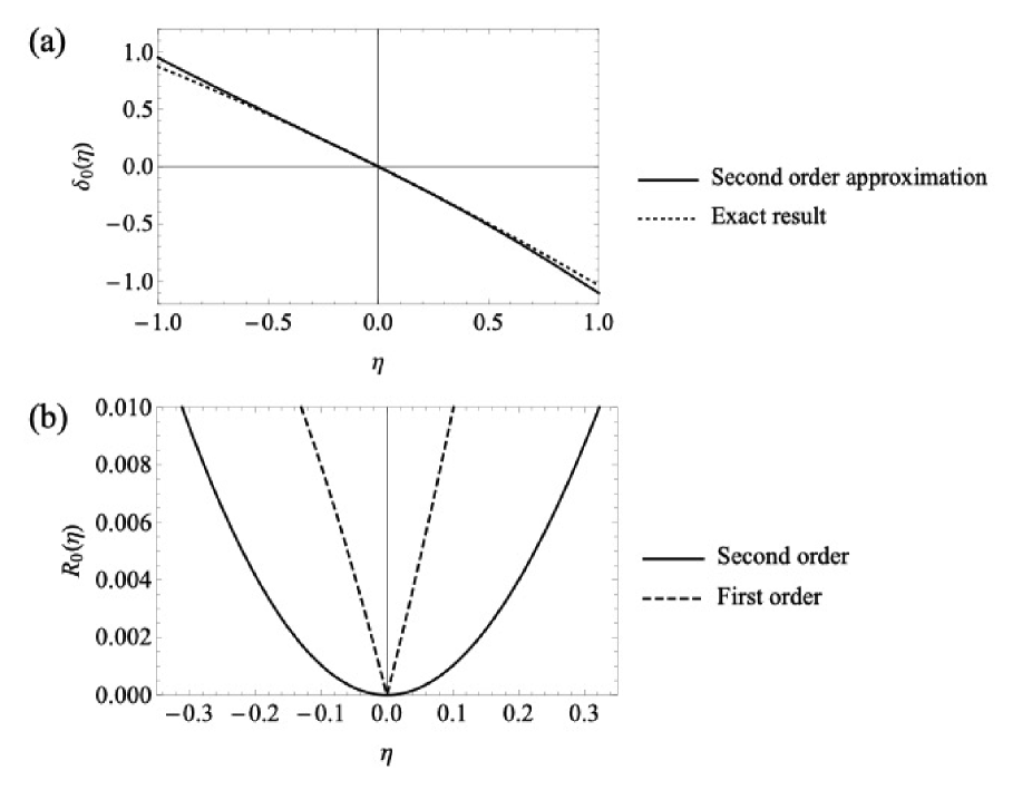
Figure 1: (a) Total phase shift to second order for $l=0,$ $\kappa=10,$ (b) relative error in the result.

For $l=5,$ $\kappa=10,$ we find a similar region to the $l=0$ case over which the approximation is useful, shown in figure 2.

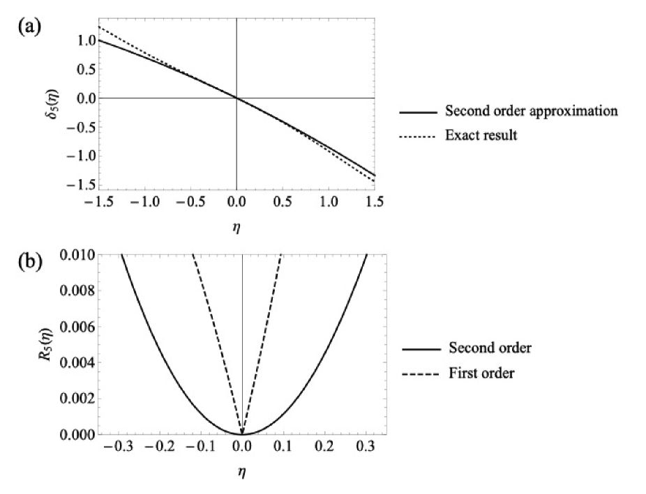
Figure 2: (a) Total phase shift to second order for $l=5,$ $\kappa=10,$ (b) relative error in the result.

As is typical for short-range potentials, the phase shifts fall off rapidly with $l,$ so that, in practice, only a small number of $l$ values need be used for a good approximation of the cross section.

IV Perturbation around exact Coulomb solutions

As discussed in the introduction, it is well known that perturbation theory, in any of its forms, applied to the Coulomb potential,

$$V^{(C)}(r)=\frac{Z_{t}Z_{p}\alpha}{r},$$ (33)

produces divergent contributions at second and higher order in $\alpha$. Here $Z_{t}$ is the atomic number of the target, $Z_{p}$ is the atomic number of the projectile and $\alpha\cong 1/137$ is the fine structure constant.

For the unitary perturbation theory presented here, not even the first order contribution is finite. The $s$-wave ($l=0$) matrix elements of the potential are

$$V_{0}^{(C)}(k_{1},k_{2})=\int_{0}^{\infty}dr\,\sqrt{\frac{2}{\pi}}\,\sin(k_{1}r)\frac{Z_{t}Z_{p}\alpha}{r}\sqrt{\frac{2}{\pi}}\,\sin(k_{1}r)=\frac{Z_{t}Z_{p}\alpha}{2\pi}\ln\left(\frac{(k_{1}+k_{2})^{2}}{(k_{1}-k_{2})^{2}}\right).$$ (34)

Clearly $V_{0}^{(C)}(p,p)$ diverges for all $p.$

However, the exact solutions of the Coulomb problem,

$$\{-\frac{1}{2m}\frac{d^{2}}{dr^{2}}+\frac{l(l+1)}{2mr^{2}}+\frac{Z_{t}Z_{p}\alpha}{r}\}y_{l}^{(C)}(r,p)=\frac{p^{2}}{2m}y_{l}^{(C)}(r,p),$$ (35)

are known (Messiah (1961)). They are real and given by

$$y_{l}^{(C)}(r,p)=\sqrt{\frac{2}{\pi}}\,c_{l}(\eta^{C}(p))\,e^{ipr}\,(pr)^{l+1}\,F(l+1+i\eta^{C}(p),2l+2;-2ipr),$$ (36)

in terms of a degenerate hypergeometric function, $F,$ (Gradsteyn and Ryzhik (1980), their section 9.21. They use the notation $F\rightarrow\Phi.$). The coefficients are

$$c_{0}=\left(\frac{2\pi\eta}{e^{2\pi\eta}-1}\right)^{\frac{1}{2}}$$ (37)

and, for $l\geq 1,$

$$c_{l}=\frac{c_{0}}{(2l+1)!!}\prod_{s=1}^{l}\left(1+\frac{\eta^{2}}{s^{2}}\right)^{\frac{1}{2}}.$$ (38)

These solutions are orthonormalized to

$$\int_{0}^{\infty}dr\,y_{l}^{(C)}(r,k_{1})y_{l}^{(C)}(r,k_{2})=\delta(k_{1}-k_{2}).$$ (39)

Here

$$\eta^{C}(p)=\frac{Z_{t}Z_{p}\alpha}{p/m}$$ (40)

is a dimensionless measure of the coupling strength. These solutions have the asymptotic behaviour, for $pr\rightarrow\infty,$

$$y_{l}^{(C)}(r,p)\rightarrow\sqrt{\frac{2}{\pi}}\,\sin(pr-\eta^{C}(p)\ln(2pr)-l\frac{\pi}{2}+\sigma_{l}(p)),$$ (41)

where the Coulomb phase shifts, $\sigma_{l}(p),$ are

$$\sigma_{l}(p)=\mathrm{Arg}(\Gamma(l+1+i\eta^{C}(p))),$$ (42)

(Messiah (1961)).

We propose perturbing around these solutions for a potential

$$V(r)=\frac{Z_{t}Z_{p}\alpha}{r}+V^{+}(r)$$ (43)

that includes the Coulomb potential and a perturbation, $V^{+}(r).$ This situation is commonly encountered in nuclear scattering of charged particles, where they interact through the Coulomb potential and also a short range nuclear contribution. We note that $V^{+}(r)$ must be in the class for which this perturbation theory is applicable, which will be the same class as for perturbation around free spherical waves, discussed in section II. In particular, $V^{+}(r)$ must vanish faster than $1/r$ as $r\rightarrow\infty.$

So we take

$$H_{0}=-\frac{1}{2m}\frac{d^{2}}{dr^{2}}+\frac{l(l+1)}{2mr^{2}}+\frac{Z_{t}Z_{p}\alpha}{r}$$ (44)

as the unperturbed Hamiltonian and develop the unitary perturbation theory for this problem, with full Hamiltonian

$$H=H_{0}+V^{+}.$$ (45)

Results are written in terms of the potential matrix elements

$$\mathscr{\mathcal{V}}_{l}(k_{1},k_{2})=\frac{\pi}{\lambda^{+}}\int_{0}^{\infty}dr\,y_{l}^{(C)}(r,k_{1})V^{+}(r)y_{l}^{(C)}(r,k_{2}),$$ (46)

which will always converge for the abovementioned constraints on $V^{+}.$

In Appendix B, we show that the presence of the logarithmic phase, $-\eta(p)\ln(2pr),$ and the Coulomb phase shifts, $\sigma_{l}(p),$ in the asymptotic form given in eq. (41) does not prevent us from obtaining results very similar to those of eq. (24). The asymptotic forms of the solutions to second order in $\eta^{+}$ take the forms

$$y_{l}^{(C)}(r,p)\rightarrow\sqrt{\frac{2}{\pi}}\,\sin(pr-\eta^{C}(p)\ln(2pr)-l\frac{\pi}{2}+\sigma_{l}(p)+\delta_{l}^{(+)}(p)),$$ (47)

with

$$\delta^{(+)}(p)\cong\delta_{l}^{(+,1)}(p)+\delta_{l}^{(+,2)}(p)$$ (48)

and

$$\delta_{l}^{(+,1)}(p) =-\eta^{+}\mathcal{V}_{l}(p,p),$$

$$\delta_{l}^{(+,2)}(p) =\eta^{+2}(\Delta_{-}^{(+)}(l,p)+\Delta_{+}^{(+)}(l,p)+\Delta_{\infty}^{(+)}(l,p)),$$ (49)

with

$$\Delta_{-}^{(+)}(l,p) =\frac{2}{\pi}\int_{-1}^{1}dx\,\frac{\{\mathcal{V}_{l}(p,p(1+x))^{2}-\mathcal{V}_{l}(p,p(1-x))^{2}\}}{x(4-x^{2})},$$

$$\Delta_{+}^{(+)}(l,p) =-\frac{1}{\pi}\int_{-1}^{1}dx\,\frac{\{\mathcal{V}_{l}(p,p(1+x))^{2}+\mathcal{V}_{l}(p,p(1-x))^{2}\}}{4-x^{2}},$$

$$\Delta_{\infty}^{(+)}(l,p) =\frac{2}{\pi}\int_{2}^{\infty}dz\,\frac{\mathcal{V}_{l}(p,pz)^{2}}{z^{2}-1}.$$ (50)

Here

$$\eta^{+}=\frac{\lambda^{+}}{p/m}.$$ (51)

Again, all of these integrals will always converge for potentials in the restricted class. The solutions are real, as will be the case at all orders.

V Example: Spherical well nuclear potential

A simple model used in nuclear physics takes the internuclear potential to be the sum of a Coulomb potential and a spherical well of the form considered in section III . Our aim was to construct a realistic description of a proton incident on a nuclear target. The first choice was $\eta^{+}=-1,$ a significant interaction strength at the limits of applicability of our perturbation theory. Nuclear potential well depths have been measured for a large number of isotopes using slow neutron scattering (Czachor and Pęczkowski (2011)). From that reference, Helium-4 ($Z_{t}=2$) was selected as the target, with a potential height of $V_{0}=-30.2\,\mathrm{MeV}$. Incident on the target is a proton of momentum $p=237\,\mathrm{MeV}$ ($E=29.5\,\mathrm{MeV}$).

From the reduction of the scattering of two particles to that of a single projectile on a fixed target, the mass must be replaced by the reduced mass in the expressions for $\eta^{+}$ and $\eta^{C}:$

$$m\rightarrow\mu=\frac{m_{\mathrm{He}}m_{p}}{m_{\mathrm{He}}+m_{p}}=749\,\mathrm{MeV}.$$ (52)

Then the relevant quantity to determine the velocity is $p/\mu.$ This gives a velocity of $\beta=v/c=0.302.$ Then the gamma factor is $\gamma=1.05.$ One limitation of the model is that this velocity enters slightly into the relativistic regime. Absent are relativistic corrections, which would be at the $5\,\%$ level. The other main limitation is modelling the nuclear potential as a spherical well.

An estimate of the nuclear radius comes from Czachor and Pęczkowski (2011)

$$R=1.3\,\mathrm{fm}\,A^{\frac{1}{3}}=2.06\,\mathrm{fm},$$ (53)

where $A=4$ is the mass number. For consistency with the equations

$$\kappa=pR,\quad V_{0}=\frac{\lambda^{+}}{R},\quad\eta^{+}=\frac{\lambda^{+}}{p/\mu}\quad\mathrm{and}\quad\eta^{C}=\frac{Z_{t}Z_{p}\alpha}{p/\mu},$$ (54)

we find

$$\kappa=2.48,\quad\lambda^{+}=-0.316,\quad\eta^{C}=0.0461.$$ (55)

Our numerical calculations give the phase shifts at first and second order, and the total, in table 1. We compare these to the exact phase shifts for the spherical well only, with these model parameters.

$l$	$\delta_{l}^{(+,1)}$	$\delta_{l}^{(+,2)}$	$\delta_{l}^{(+,1)}+\delta_{l}^{(+,2)}$	$\delta_{l}^{\mathrm{exact}}$ (Nuclear)
$\ 0\$	1.230	-0.316	0.914	0.805
$\ 1\$	0.651	0.299	0.950	0.906
$\ 2\$	0.136	0.050	0.186	0.232
$\ 3\$	0.015	0.003	0.018	0.020
$\ 4\$	0.001	0.000	0.001	0.001

Table 1: First- and second-order phase shift contributions and their sum for the model parameters.

In Hoffmann (2017), a formalism was developed to describe the scattering of a Gaussian wavepacket with a momentum width, $\sigma_{p},$ small compared to the incoming average momentum, $p,$ incident on a fixed target Coulomb potential. We calculated wavepacket-to-wavepacket transition probabilities, but a simple formula presented there allows the calculation of cross sections. The fact that a probability can never rise greater than unity was responsible for the observation that the Coulomb probability takes a finite value in the forward direction. Calculation of plane wave scattering predicts a divergence in the forward direction.

It is a simple matter to adapt this formalism to the model considered here. This treatment, with a Coulomb potential included, is expected to avoid a singularity in the forward direction. We chose the momentum width relative to the incident average momentum such that

$$\epsilon=\frac{\sigma_{p}}{p}=0.001.$$ (56)

The formula we used for the differential cross section (including the behaviour around the forward direction), modified from Hoffmann (2017) to include the nuclear phase shifts, is

$$\frac{d\sigma^{+}}{d\Omega}=\frac{1}{4p^{2}}\left|\sum_{l=0}^{\infty}(2l+1)e^{-2\epsilon^{2}(l+\frac{1}{2})^{2}}e^{i2\sigma_{l}(p)}e^{i2(\delta_{l}^{(+,1)}(p)+\delta_{l}^{(+,2)}(p))}P_{l}(\cos\theta)\right|^{2}.$$ (57)

(We ignored time delays/advancements.) This has been tested to give a cross section in very close agreement with the Rutherford cross section (for $\delta_{l}^{(+,1)}(p)+\delta_{l}^{(+,2)}(p)=0$), except close to $\theta=0,$ where a finite result is predicted.

A numerical problem arose. If this sum was evaluated as written, the resulting cross section appeared to include only the Coulomb part. It was necessary to use the identity

$$e^{i2\delta_{l}}=1+2i\,e^{i\delta_{l}}\,\sin(\delta_{l}),$$ (58)

with

$$\delta_{l}=\delta_{l}^{(+,1)}(p)+\delta_{l}^{(+,2)}(p)$$ (59)

to separate the sum into two parts. Adding the resulting sums and taking the modulus-squared gave a differential cross section with both Coulomb and nuclear contributions.

First we plot (in fig. 3) the differential cross section for the nuclear spherical well only, using the exact phase shifts with our model parameters, for comparison. We used

$$\frac{d\sigma_{\mathrm{s}}^{N}}{d\Omega}=\frac{1}{p^{2}}\left|\sum_{l=0}^{l_{\mathrm{max}}}(2l+1)\,e^{i\delta_{l}^{\mathrm{exact}}}\sin(\delta_{l}^{\mathrm{exact}})\,P_{l}(\cos\theta)\right|^{2},$$ (60)

with $l_{\mathrm{max}}=4.$ Note $\exp(-2\epsilon^{2}(l+\frac{1}{2})^{2})=1+\mathcal{O}(\epsilon^{2}).$ This formula also comes from using the separation in eq. (58) and leaves out the strong, narrow contribution around the forward direction, although we plotted it in figure 3. The wavepacket formalism adds nothing here except smearing over the angular scale $\Delta\theta\sim 0.001$ and that narrow peak around $\theta=0$, not a delta function but a function of the form

$$\frac{d\sigma_{\mathrm{forward}}^{N}}{d\Omega}=\frac{1}{16p^{2}}\frac{1}{\epsilon^{4}}\,e^{-\theta^{2}/4\epsilon^{2}}.$$ (61)

We display the cross sections in barns ($1\,\mathrm{barn}=10^{-28}\,\mathrm{m}^{2}=100\,\mathrm{fm^{2}}$) and the momentum in MeV, including the strong, narrow contributions around the forward direction. If

$$\frac{d\sigma}{d\Omega}=\frac{1}{p^{2}}f$$

in Heaviside-Lorentz units, the conversion is given by

$$\frac{d\sigma}{d\Omega}[\mathrm{barn}]=\frac{389}{p[\mathrm{MeV}]^{2}}f.$$

Figure 3: Differential cross section for spherical well only: exact solution with model parameters.

In fig. 4, we plot (on the same scale as that of fig. (3) the cross section for the Coulomb interaction alone, compared to the Rutherford Coulomb result (Messiah (1961); Rutherford (1911)),

$$\frac{d\sigma}{d\Omega}|_{\mathrm{Rutherford}}[\mathrm{barn}]=\frac{389}{p[\mathrm{MeV}]^{2}}\frac{\eta^{C2}}{4\sin^{4}(\frac{\theta}{2})}.$$

No separation is used here. The Coulomb cross section does not generally separate into a narrow forward peak and a finite contribution around $\theta=0,$ as seen for shorter-range potentials, as we saw in Hoffmann (2017). This case is an exception, in the regime of low interaction strength, where the cross section is dominated by the essentially free contribution close to the origin.

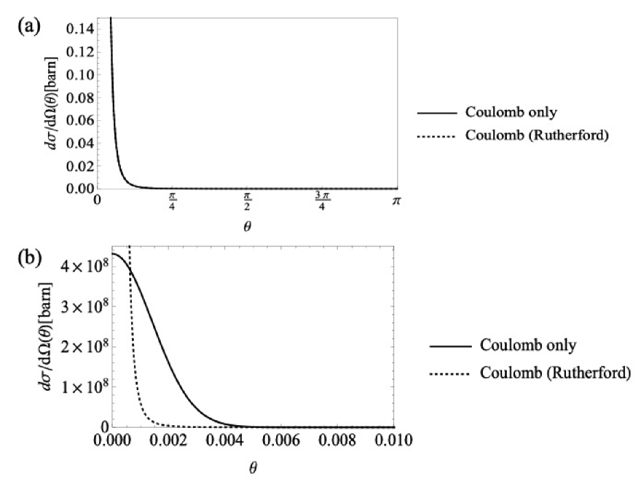
Figure 4: Differential cross section for the Coulomb interaction only, with model parameters.

Results for the Coulomb plus nuclear model are show in fig. 5. We see that the model cross section is significantly larger than the Rutherford cross section at large angles. It is approximately the incoherent sum of the nuclear and Coulomb parts at angles greater than $\pi/4.$ At lower angles, the difference is larger, so an interference term must be contributing significantly. We show the cross section at low angles, where the wavepacket treatment guarantees finiteness. The Rutherford result, derived classically, does not include that constraint, but pure Coulomb cross sections with the wavepacket treatment were also found to be finite at $\theta=0$ in Hoffmann (2017), for a range of different parameters.

Votta et al. (Votta et al. (1974)) measured the differential cross section for protons on $\phantom{|}{}_{2}^{4}\mathrm{He}$ at an incident kinetic energy of $E_{V}=85\,\mathrm{MeV}$ ($p_{V}=408\,\mathrm{MeV}$). The peak seen in figure 5 is at about $0.07\,\mathrm{b}.$ If we simply adjust this for the difference in momentum by

$$\left(\frac{p}{p_{V}}\right)^{2}0.07\,\mathrm{b}=\left(\frac{237}{408}\right)^{2}0.07\,\mathrm{b}=24\,\mathrm{mb},$$

we find a value well within the significant region of their measurements. It is remarkable that such a crude representation of the nuclear potential leads to results of the correct order of magnitude.

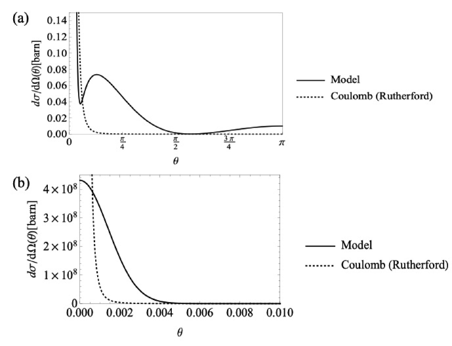
Figure 5: Differential cross section in barns as a function of angle, compared to the Rutherford result.

VI Conclusions

We have constructed a perturbation theory to treat interactions that can include the Coulomb interaction, such as is encountered in nuclear physics. The Coulomb part is not treated perturbatively; the exact solutions are employed.

The first task was to extend the perturbation theory for non-Coulomb interactions from the case where the angular momentum quantum number was $l=0$ (the only case considered in Hoffmann (2021)) to general nonnegative integers, $l.$ The method was tested on a system with an exact solution, up to second order in the perturbation, for $l=0$ and $l=5$. As expected, an $\mathcal{O}(\eta^{3})$ error was found in both cases, where $\eta$ is the dimensionless coupling strength (eq. (23)). Analysis of the second-order terms in the series shows that we expect finiteness for general potentials, provided their singularity at the origin is less than $1/r^{2}$ and that they fall off asymptotically with $r$ faster than $1/r.$

Subsequently, the method for the sum of a Coulomb potential and a perturbing potential was developed, and found to have similarities with the non-Coulomb method. A model system was simulated, involving a Coulomb interaction and a spherical well, the latter being a primitive representation of a nuclear interaction. The differential cross section for scattering from this potential was calculated, using the wavepacket formalism of Hoffmann (2017). The physically realistic result differs from the incoherent sum of Coulomb and nuclear cross sections, as expected. The magnitudes of the differential cross sections were realistic.

Again, the second-order terms in the perturbation series were finite. Analysis shows that they would continue to be finite for general perturbing potentials in the class of sufficiently well-behaved potentials that we have defined. We conjecture that the terms would remain finite at third and higher order. This is the central result of this paper: a finite perturbation theory that can include the Coulomb potential. In contrast, applying perturbation theory directly to the Coulomb potential gives infinities.

Appendix A Evaluation of integrals for perturbation about the free solutions

In Hoffmann (2021) we derived results only for the case $l=0.$ Here we evaluate integrals that we will need for general $l=0,1,2,\dots$

The asymptotic form of the free spherical waves is (Messiah (1961))

$$y_{l}^{(0)}(r,k)\rightarrow\sqrt{\frac{2}{\pi}}\,\sin(kr-l\frac{\pi}{2})$$ (62)

as $kr\rightarrow\infty.$ We will find two types of principal part integrals that we will need to evaluate in the same asymptotic limit:

$$I_{1} =P\int_{0}^{\infty}dk\,\sqrt{\frac{2}{\pi}}\,\sin(kr-l\frac{\pi}{2})\frac{f(k)}{k^{2}-p^{2}},$$

$$I_{2} =P\int_{0}^{\infty}dk\,\sqrt{\frac{2}{\pi}}\,\cos(kr-l\frac{\pi}{2})\frac{f(k)}{k^{2}-p^{2}}.$$ (63)

Here $f(k)$ is analytic on the integration region and is such that the integrals always converge.

We separate these into integrals on $k\in[0,2p]$ and integrals on $k\in[2p,\infty).$ For the finite integration region, we define $k=p(1+x)$ and $\kappa=pr,$ and use

$$\sin(\kappa-l\frac{\pi}{2}+\kappa x) =\sin(\kappa-l\frac{\pi}{2})\cos(\kappa x)+\cos(\kappa-l\frac{\pi}{2})\sin(\kappa x),$$

$$\cos(\kappa-l\frac{\pi}{2}+\kappa x) =\cos(\kappa-l\frac{\pi}{2})\cos(\kappa x)-\sin(\kappa-l\frac{\pi}{2})\sin(\kappa x).$$ (64)

Also for the integrals on $x\in[-1,1],$ we separate the integrands into parts even and odd in $x.$ The latter will vanish under principal part integration, including when the integrand has a $1/x$ singularity. The remaining integrand will be free from singularities and standard integration can be used. The two integrals on $k\in[2p,\infty)$ have no singularities on that region, so reduce to standard integrals. It will then suffice to consider

$$I_{\mathrm{0}} =\int_{-1}^{1}dx\,\frac{\sin(\kappa x)}{x}f_{+}(x),$$

$$I_{s,F} =\int_{-1}^{1}dx\,\sin(\kappa x)f_{+}(x),\quad I_{c,F}=\int_{-1}^{1}dx\,\cos(\kappa x)f_{+}(x),$$

$$I_{s,I} =\int_{2}^{\infty}dz\,\sin(pz)\,g(z),\quad I_{c,I}=\int_{2}^{\infty}dz\,\cos(pz)\,g(z)$$ (65)

where $f_{+}(x)$ is even in $x$ and satisfies our regularity and convergence requirements. For the infinite integration region, we used $k=pz.$ Here $g(z)$ must decrease at least as fast as $1/z$ for convergence.

In the first of these integrals, the functions

$$\Delta(x,\kappa)=\frac{\sin(\kappa x)}{x}$$ (66)

have peak value $\Delta(0,\kappa)=\kappa\gg 1$ and fall off like $1/x,$ with rapid oscillations, over a width of order $1/\kappa.$ Thus they are approximations to a delta function, the approximation improving as $\kappa\rightarrow\infty.$ They are normalized to

$$\int_{-1}^{1}dx\,\frac{\sin(\kappa x)}{x}=\pi+\mathcal{O}(\frac{1}{\kappa}).$$ (67)

So we expect

$$\Delta(x,\kappa)\rightarrow\pi\,\delta(x)$$ (68)

as $\kappa\rightarrow\infty.$

Hence we expect $I_{\mathrm{0}}=\pi f_{+}(0).$ Integration by parts applied to the remaining integrals shows that they will vanish like order $1/\kappa.$ We verified the $I_{\mathrm{0}}$ result numerically, using polynomials in $x^{2}$ for $f_{+}(x).$

We find that together these results give the asymptotic forms

$$P\int_{0}^{\infty}dk\,\sqrt{\frac{2}{\pi}}\,\sin(kr-l\frac{\pi}{2})\frac{f(k)}{k^{2}-p^{2}}\rightarrow\{\frac{\pi}{2p}f(p)\}\sqrt{\frac{2}{\pi}}\,\cos(pr-l\frac{\pi}{2})$$ (69)

and

$$P\int_{0}^{\infty}dk\,\sqrt{\frac{2}{\pi}}\,\cos(kr-l\frac{\pi}{2})\frac{f(k)}{k^{2}-p^{2}}\rightarrow\{-\frac{\pi}{2p}f(p)\}\sqrt{\frac{2}{\pi}}\,\sin(pr-l\frac{\pi}{2}).$$ (70)

Appendix B Evaluation of integrals for perturbation about the Coulomb solutions

The asymptotic form of the Coulomb wavefunctions as $kr\rightarrow\infty$ is (Messiah (1961))

$$y_{l}^{(C)}(r,k)=\sqrt{\frac{2}{\pi}}\,\sin(kr-\eta(k)\ln(2kr)-l\frac{\pi}{2}+\sigma_{l}[\eta(k)]),$$ (71)

with

$$\eta(k)=\frac{Z_{t}Z_{p}\,\alpha}{k/m}.$$ (72)

This asymptotic form differs from the free case by the presence of the logarithmic phase, $-\eta(k)\ln(2kr),$ and the Coulomb phase shifts, $\sigma_{l}[\eta(k)].$ It is not obvious that we will be able to obtain results similar to those just derived for the free case.

The phase

$$\varphi_{l}(r,k)=kr-\eta(k)\ln(2kr)-l\frac{\pi}{2}+\sigma_{l}[\eta(k)]$$ (73)

has derivative

$$\frac{\partial\varphi_{l}(r,k)}{\partial k}=r+\frac{Z_{t}Z_{p}\,\alpha m}{k^{2}}\{\ln(\frac{2kr}{e})-\mathrm{Re}(\psi(l+1+i\eta(k)))\}.$$ (74)

We used (Messiah (1961))

$$e^{i2\sigma_{l}(k)}=\frac{\Gamma(l+1+i\eta(k))}{\Gamma(l+1-i\eta(k))}$$ (75)

and

$$\psi(z)=\frac{1}{\Gamma(z)}\frac{d\Gamma(z)}{dz},$$ (76)

the psi or Polygamma function (Gradsteyn and Ryzhik (1980), their section 8.36).

This first derivative will generally be large because of the presence of $r,$ giving a rapidly oscillating sine function, but the phase has a stationary point where

$$1+\frac{Z_{t}Z_{p}\,\alpha}{v^{2}\rho}\{\ln(\frac{2v\rho}{e})-\mathrm{Re}(\psi(l+1+i\frac{Z_{t}Z_{p}\,\alpha}{v}))\}=0,$$ (77)

where

$$v=\frac{k}{m},\quad\rho=mr,$$ (78)

both dimensionless. In the neighbourhood of the stationary point, the phase varies slowly and we will find an undesired finite contribution to the integrals we will consider (those in parallel to eqs. (65)).

We find that the root of eq. (77), $v_{0}(\rho),$ approaches zero from above as $\rho\rightarrow\infty.$ The state vector with $k=0$ is unphysical in our theory. It has a wavefunction independent of $r$ to which we cannot apply continuum normalization. Hence we argue that the stationary point should have no physical effect as $\rho\rightarrow\infty.$ Numerically, it is a simple matter to remove its contribution for finite $r$. We find a small region, $v\in[0,\epsilon(\rho)],$ containing the stationary point, with, say $\epsilon(\rho)=2v_{0}(\rho),$ and remove that region from the integrals. In terms of $x,$ this region is $x\in[-1,-1+\frac{2\epsilon(\rho)}{p/m}].$

We want to evaluate integrals similar to those in eq. (65). We define

$$\Delta\varphi_{l}(\rho,v,x)=\varphi_{l}(r,p(1+x))-\varphi_{l}(r,p)$$ (79)

so that the Taylor series around $x=0$ is

$$\Delta\varphi_{l}(\rho,v,x)=px\frac{\partial\varphi_{l}(r,k)}{\partial k}|_{k=p}+\mathcal{O}(x^{2}).$$ (80)

This gives integrals that are linear combinations of $\sin(\varphi_{l}(r,p))$ and $\cos(\varphi_{l}(r,p)).$ So we need to evalute the remaining integrals of the form

$$I_{\mathrm{0}}^{(C)} =\int_{-1}^{1}dx\,\frac{\sin(\Delta\varphi_{l}(\rho,v,x))}{x}f_{+}(x),$$

$$I_{s,F}^{(C)} =\int_{-1}^{1}dx\,\sin(\Delta\varphi_{l}(\rho,v,x))f_{+}(x),\quad I_{c,F}^{(C)}=\int_{-1}^{1}dx\,\cos(\Delta\varphi_{l}(\rho,v,x))f_{+}(x),$$

$$I_{s,I}^{(C)} =\int_{2}^{\infty}dz\,\sin(\Delta\varphi_{l}(\rho,v,x))\,g(z),\quad I_{c,I}^{(C)}=\int_{2}^{\infty}dz\,\cos(\Delta\varphi_{l}(\rho,v,x))\,g(z),$$ (81)

with the above conditions on $f_{+}(x)$ and $g(z).$ We find that the last four integrals all vanish like $1/v\rho=1/pr$ as $pr\rightarrow\infty.$

Since the dominant term in the phase derivative gives

$$px\frac{\partial\varphi_{l}(r,k)}{\partial k}|_{k=p}\sim prx,$$ (82)

we define

$$\Delta\varphi_{l}(\rho,v,x)=prx+\delta\varphi_{l}(\rho,v,x),$$ (83)

giving

$$I_{0}^{(C)}=\int_{-1}^{1}dx\,\frac{\sin(v\rho x)}{x}F_{+}(x)+\int_{-1}^{1}dx\,\cos(v\rho x)G_{+}(x),$$ (84)

with

$$F_{+}(x) =[\cos(\delta\varphi_{l}(v,\rho,x))]_{+}f_{+}(x),$$

$$G_{+}(x) =\frac{[\sin(\delta\varphi_{l}(v,\rho,x))]_{-}}{x}f_{+}(x).$$ (85)

We apply integration by parts to both terms, giving

$$I_{0}^{(C)}=\{\pi f_{+}(0)+2\mathrm{si}(v\rho)F_{+}(1)\\ \quad-2\int_{0}^{1}dx\,\mathrm{si}(v\rho x)\,F_{+}^{\prime}(x)\}+\{\frac{2G_{1}(1)\sin(v\rho x)}{v\rho}-\frac{1}{v\rho}\int_{0}^{1}dx\,\sin(v\rho x)\,G_{+}^{\prime}(x)\},$$ (86)

where (Gradsteyn and Ryzhik (1980), their section 8.23)

$$\mathrm{si}(z)=-\int_{z}^{\infty}dt\,\frac{\sin t}{t}.$$ (87)

We note $\mathrm{si}(v\rho)\sim\mathcal{O}(1/v\rho)$ as $v\rho\rightarrow\infty.$

We encountered difficulties trying to numerically integrate the integrals in eq. (81) directly. The problem is integrands with rapidly oscillatory behaviour. This analytic treatment leads to two remainders,

$$R_{1}=-2\int_{0}^{1}dx\,\mathrm{si}(v\rho x)\,F_{+}^{\prime}(x)\quad\mathrm{and}\quad R_{2}=-\frac{1}{v\rho}\int_{0}^{1}dx\,\sin(v\rho x)\,G_{+}^{\prime}(x),$$ (88)

both of which could be numerically integrated. Both were found to vanish as $v\rho\rightarrow\infty.$ So we find

$$\lim_{pr\rightarrow\infty}I_{\mathrm{sinc}}^{(C)}=\pi f_{+}(0).$$ (89)

Using these results, we find

$$P\int_{0}^{\infty}dk\,\sqrt{\frac{2}{\pi}}\,\sin(kr-\eta(k)\ln(2kr)-l\frac{\pi}{2}+\sigma_{l}[\eta(k)])\frac{f(k)}{k^{2}-p^{2}}\rightarrow\\ \{\frac{\pi}{2p}f(p)\}\sqrt{\frac{2}{\pi}}\,\cos(pr-\eta(p)\ln(2pr)-l\frac{\pi}{2}+\sigma_{l}[\eta(p)])$$ (90)

and

$$P\int_{0}^{\infty}dk\,\sqrt{\frac{2}{\pi}}\,\cos(kr-\eta(k)\ln(2kr)-l\frac{\pi}{2}+\sigma_{l}[\eta(k)])\frac{f(k)}{k^{2}-p^{2}}\rightarrow\\ \{-\frac{\pi}{2p}f(p)\}\sqrt{\frac{2}{\pi}}\,\sin(pr-\eta(p)\ln(2pr)-l\frac{\pi}{2}+\sigma_{l}[\eta(p)]),$$ (91)

where $f(k)$ is regular on the integration region and such that the integrals always converge.

Data sharing is not applicable to this article as no new data were created or analyzed in this study.

References

Deltuva et al. (2005)A. Deltuva, A. C. Fonseca, A. Kievsky,
S. Rosati, P. U. Sauer, and M. Viviani, Phys.
Rev. C 71, 064003
(2005).
Abramowitz and Stegun (1972)M. Abramowitz and I. A. Stegun, Handbook of Mathematical
Functions, 9th ed. (Dover,
N. Y., 1972).
Gradsteyn and Ryzhik (1980)I. S. Gradsteyn and I. M. Ryzhik, Tables of Integrals,
Series and Products, corrected and enlarged ed. (Academic Press, Inc., San Diego, CA, 1980).
Czachor and Pęczkowski (2011)A. Czachor and P. Pęczkowski, Phys. Part. Nucl. Lett. 8 (2011).