A Case against a Significant Detection of Precession in the Galactic Warp

Abstract

Recent studies of warp kinematics using Gaia DR2 data have produced detections of warp precession for the first time, which greatly exceeds theoretical predictions of models. However, this detection assumes a warp model derived for a young population (few tens of megayears) to fit velocities of an average older stellar population of the thin disk (several gigayears) in Gaia-DR2 observations, which may lead to unaccounted systematic errors. Here, we recalculate the warp precession with the same approach and Gaia DR2 kinematic data, but using different warp parameters based on the fit of star counts of the Gaia DR2 sample, which has a much lower warp amplitude than the young population. When we take into account this variation of the warp amplitude with the age of the population, we find that there is no need for precession. We find the value of warp precession $\beta=4^{+6}_{-4}$ km s^-1 kpc^-1, which does not exclude nonprecessing warp.

tablenum SIXtablenum

1 Introduction

Although the warp was discovered over 60 yr ago (Kerr, 1957; Oort et al., 1958) and extensively studied in the past decades (Carney & Seitzer, 1993; López-Corredoira et al., 2002b; Amôres et al., 2017; Chen et al., 2019, and others), the mechanism causing the warp is still unknown. Theories include accretion of intergalactic matter onto the disk (López-Corredoira et al., 2002a), interaction with other satellites (Kim et al., 2014), the intergalactic magnetic field (Battaner et al., 1990), a misaligned rotating halo (Debattista & Sellwood, 1999), and others.

Kinematic studies are necessary in order to reveal the origin of the warp, as different models give different predictions. Warp precession is estimated by various mechanisms of warp formation, such as torque of the dark halo on the disk (Dubinski & Chakrabarty, 2009), torque on the disk due to misalignment of the halo and the disk (Jiang & Binney, 1999), or accretion of intergalactic matter onto the disk (López-Corredoira et al., 2002a; Jeon et al., 2009).

Recently, studies of warp kinematics and time evolution were made in order to understand the origin of the warp (Poggio et al., 2018, 2020; Wang et al., 2020). In particular, the result of Poggio et al. (2020, hereafter P20) is of great interest as they measured the precession of the Galactic warp for the first time. Using the second Gaia data release DR2 (Gaia Collaboration et al., 2016, 2018) combined with Two Micron All-Sky Survey (Skrutskie et al., 2006, 2MASS) photometry, they find the warp precession to be $\beta=10.86\pm 0.03(stat.)\pm 3.20(syst.)$ km s^-1 kpc^-1. Their result was supported by another recent work of Cheng et al. (2020), who measured a similar value of precession $\beta=13.57^{+0.20}_{-0.18}$ km s^-1 kpc^-1 by fitting vertical velocities using data from Gaia DR2 and Apache Point Observatory Galactic Evolution Experiment 2 (Majewski et al., 2017, APOGEE-2), as contained in Sloan Digital Sky Survey (SDSS) Data Release 16 (Ahumada et al., 2020, DR16). These results greatly exceed predictions of warp precession estimated considering various mechanisms of warp formation, such as torque of the dark halo on the disk (Dubinski & Chakrabarty, 2009), torque on the disk due to misalignment of the halo and the disk (Jiang & Binney, 1999), or accretion of intergalactic matter onto the disk (López-Corredoira et al., 2002a; Jeon et al., 2009). All these works predict a small value of precession, between $0.1$ and $1.5$ km s^-1 kpc^-1. The result of P20 contradicts conclusions of dynamical models of warp formation and suggests that warp is a transient response of the disk to an outside interaction rather than a slowly evolving structure. We know that most spiral galaxies have warps (Reshetnikov & Combes, 1998; Sánchez-Saavedra et al., 2003), so it seems unlikely that the warp is caused by a transient phenomenon in all of them unless they all have a substructure that triggers warp formation very often.

Kinematics studies also discovered significant substructures in the disk velocities (Wang et al., 2018; López-Corredoira et al., 2020; Xu et al., 2020). In López-Corredoira et al. (2020) it is shown that the features in vertical motions can be partially explained by the warp; however, the main observed features can only be explained in terms of out-of-equilibrium models. Nevertheless, our purpose in this paper is not to explain all the features of the observed velocities, but just to verify that a simple warp model without precession is able to fit the data, against the claims of P20. Therefore, we will consider the substructures as random fluctuations and focus only on the large structural effect of the warp.

In this work, we challenge the result of P20, as we think they did not consider the variation of the amplitude of the warp with the age of the population, and present our own calculation of the warp precession rate. P20 derived the warp precession under an assumption that the amplitude of the warp corresponding to specific stellar populations (Classical Cepheids, Pulsars) is representative of the whole population. This is not consistent with data, as the stellar population traced by the Gaia survey is significantly older on average ($\sim$5-6 Gyr) and it presents a much lower amplitude of the warp than the young population one (Chrobáková et al., 2020; Wang et al., 2020). For simplicity, we will refer to this population as an “old population” and to Cepheids as a “young population.” We show that when applying the warp model for an old population we cannot detect the precession of the warp; therefore, we cannot favor any model of warp formation.

2 Data selection

We use the data of López-Corredoira & Sylos-Labini (2019, hereafter LS19), who have produced extended kinematic maps of the Milky Way by using Gaia DR2, by considering stars with measured radial heliocentric velocities and with parallax errors less than $100\%$; the total sample contains 7,103,123 sources. Such objects were observed by the Radial Velocity Spectrometer (RVS; Cropper et al., 2018) that collects medium-resolution spectra (spectral resolution $\frac{\lambda}{\Delta\lambda}\approx 11700$) over the wavelength range 845-872 nm, centered on the Calcium triplet region. Radial velocities are averaged over a 22 month time span of observations. Most sources have a magnitude brighter than 13 in the $G$ filter.

In more detail, the effective temperatures for the sources with radial velocities that LS19 have considered are in the range of 3550 to 6900 K. The uncertainties of the radial velocities are 0.3 km s^-1 at $G_{\mathrm{RVS}}<8$, 0.6 km s^-1 at $G_{\mathrm{RVS}}=10$, and 1.8 km s^-1 at $G_{\mathrm{RVS}}=11.75$; plus systematic radial velocity errors of $<0.1$ km s^-1 at $G_{\mathrm{RVS}}<9$ and 0.5 km s^-1 at $G_{\mathrm{RVS}}=11.75$. The uncertainties of the parallax are 0.02 –0.04 mas at $G<15$, 0.1 mas at $G=17$, 0.7 mas at $G=20,$ and 2 mas at $G=21$. The uncertainties of the proper motion are 0.07 mas $\mathrm{yr}^{-1}$ at $G<15$, 0.2 mas $\mathrm{yr}^{-1}$ at $G=17$, 1.2 mas $\mathrm{yr}^{-1}$ at $G=20,$ and 3 mas $\mathrm{yr}^{-1}$ at $G=21$. For details on radial velocity data processing and the properties and validation of the resulting radial velocity catalog, see Sartoretti et al. (2018) and Katz et al. (2019). The set of standard stars that was used to define the zero-point of the RVS radial velocities is described in Soubiran et al. (2018). LS19 consider the zero-point bias in the parallaxes of Gaia DR2, as found by Lindegren et al. (2018), Arenou et al. (2018), Stassun & Torres (2018), and Zinn et al. (2019); however, they find that the effect of the systematic error in the parallaxes is negligible.

As the parallax error grows as the distance from us grows, LS19 applied a statistical deconvolution of the parallax errors based on Lucy’s inversion method (Lucy, 1974) to statistically estimate the distance. In this way they have derived the extended kinematical maps in the range of Galactocentric distances up to 20 kpc.

From this sample, we only choose stars with the Galactic latitude $\lvert b\rvert<$$$, Galactocentric distance $R>12$ kpc, and heliocentric distance $r<8$ kpc, so we obtain a dataset with Galactocentric radius $12<R<16$ kpc, maximum vertical distance $z\approx 1.4$ kpc, and within $\lvert\phi\rvert<$$,$ as seen from the Galactic center. We bin the data in Galactocentric Cartesian coordinates with size $\Delta X=1.0$ kpc and $\Delta Y=1.0$ kpc. For $R<12$ kpc, the amplitude of the warp is too small to be considered and the relative error of the warp model is higher. For $r>8$ kpc, the errors of vertical velocities are very large.

3 Methods

We model the warp in Galactocentric cylindrical coordinates $(R,\phi,z)$ using the warp model of Chrobáková et al. (2020, Equation (11)) for which the average height over the plane of the Galactic disk stars $z_{w}$ is calculated as

$$z_{w}=[C_{w}R(pc)^{\epsilon_{w}}sin(\phi-\phi_{w})+17]~{}pc~{}.$$ (1)

The model describes the warp as a series of tilted rings, where the amount of tilt is the Galactocentric distance raised to a power of $\epsilon_{w}$, $C_{w}$ is the warp amplitude, and $\phi_{w}$ is the Galactocentric angle defining the warp’s line of nodes. $C_{w},\epsilon_{w}$, and $\phi_{w}$ are free parameters of the model, which were fitted in Chrobáková et al. (2020). The 17 pc term compensates for the elevation of the Sun above the plane (Karim & Mamajek, 2017). We consider time evolution of the warp amplitude and warp precession

$$C_{w}(t) = C_{w,max}sin(\omega t+\alpha)~{},$$ (2)

$$\phi_{w}(t) = \phi_{w0}+\beta t~{}.$$ (3)

The values of model parameters given by Chrobáková et al. (2020) are

$$C_{w} = 1.17\cdot 10^{-8}\mathrm{pc}\pm 1.34\cdot 10^{-9}\mathrm{pc}(stat.)$$

$${}^{+0\mathrm{pc}}_{-2.9\cdot 10^{-10}\mathrm{pc}}(syst.)~{},$$

$$\epsilon_{w} = 2.42\pm 0.76(stat.)^{+0.129}_{-0}(syst.)~{},$$ (4)

$$\phi_{w} = $$\pm$$(stat.)^{+$$}_{-$$}(syst.)~{}.$$

We follow the approach of P20, taking the zeroth moment of the collisionless Boltzmann equation to derive the expression for vertical velocity.

$$v_{z}(R,\phi) = C_{w,0}KR^{\epsilon_{w}}sin(\phi-\phi_{w,0})$$

$$- C_{w,0}R^{\epsilon_{w}}\beta cos(\phi-\phi_{w,0})$$

$$+ C_{w,0}R^{\epsilon_{w}-1}cos(\phi-\phi_{w,0})v_{\phi}~{},$$

where $C_{w,0}$ and $\phi_{w,0}$ are Eqs. (2) and (3) at present time $t$ and

$$K=\omega\cdot cotan(\alpha)~{}.$$ (6)

We use the least-squares method, to fit the data, minimizing $\chi^{2}$:

$${\chi^{2}=\sum_{i}\frac{(v^{obs}_{Z,i}-v^{model}_{Z,i})^{2}}{\sigma^{2}_{i}}~{}.}$$ (7)

López-Corredoira & Sylos-Labini (2019) give their data in coordinates $(X,Y)$ binned with size $\Delta X=0.2$ kpc and $\Delta Y=0.2$ kpc. To avoid confusion, we will refer to those bins as pixels. Each bin with average velocity $v^{obs}_{Z,i}$ is generated by grouping different pixels $(X,Y)$ into squares of $1$ kpc $\times 1$ kpc with the same number of pixels for all bins, where $\sigma^{2}_{i}$ is the error of velocity in each bin:

$${\sigma^{2}_{i}=\frac{\sum_{j\in i}w_{j}\sigma_{Z,j}^{2}}{\sum_{j\in i}w_{j}}~{},}$$ (8)

where $\sigma_{Z,j}$ is the error of velocity in the pixel $j$ and $w_{j}$ is its weight (number of stars in our case).

Errors in the bin can be calculated differently, depending on whether the statistical or systematic error dominates. We tried to calculate the error using different approaches, but we find that the results are similar in all cases. More about error estimation can be found in Section 4.3.

4 Results

4.1 Old Population Warp Does Not Give Precession

We fit the vertical velocities with a warp model considering both the evolution in time of the warp amplitude and the warp precession. As a first case, we only take data with azimuth $\lvert\phi\rvert<$$$ (near the anticenter), where the dependence of amplitude on time is negligible, as can be seen from Equation (3), when we set the value of the angle of the line of nodes. Therefore we only have one free parameter $\beta$ that represents precession of the warp azimuth of the line of nodes (see Equation (3)). We carry out the fit for the model of Chrobáková et al. (2020) and the model of P20 using the warp parameters of the linear model of Chen et al. (2019). Differences in maximum amplitude for these warp models can be seen in Figure 1. In Figure 2(a) we show the best fit and the nonprecessing warp for the model of P20. It is clear that, with the high amplitude, the nonprecessing model gives much higher velocity than what is observed, so a high precession is necessary to compensate for that. That is precisely the result of P20. In contrast, the warp model representative of the old stellar population of Gaia DR2 (Chrobáková et al., 2020) reaches about 3–4 times lower amplitude than the one used by P20 (see Figure 1); therefore, it does not need a high precession.

As shown in Figure 2(b), with a nonprecessing warp the amplitude of the velocity is already of the order of the data and the precession gives only a small correction. The value of precession we obtain with the model used by P20 is $\beta=13\pm 1$ km s^-1 kpc^-1, which is similar, although a bit higher than the value obtained by P20 ($\beta=10.86\pm 0.03(stat.)\pm 3.20(syst.)$ km s^-1 kpc^-1), probably due to difference in datasets. The value of precession using the old stellar population of Gaia DR2 is $\beta=-1\pm 9$ km s^-1 kpc^-1, which is consistent with the nonprecessing warp model, as well as with the result of P20, since we have large error bars. P20 already pointed out that a warp model with a small amplitude like ours would fit the data without the need for precession; however, they do not carry out the analysis with such a model and do not provide a result of such fit; therefore, we cannot compare our result with theirs directly.

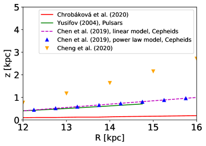
Figure 1: Comparison of maximum amplitudes of various warp models, used to calculate the precession. It is evident that the model of Chrobáková et al. (2020), derived for the whole stellar population, reaches a significantly lower amplitude than other works.

Figure 2: Result of the fit with warp models, using only data near the anticenter. The blue curve is for the nonprecessing model of the warp ($\beta=0$ km s^-1 kpc^-1), the green curve is the best fit of the data. (a) Model of P20, with the warp parameters of Chen et al. (2019). For the best fit, we find $\beta=13\pm 1$ km s^-1 kpc^-1. (b) Model of Chrobáková et al. (2020). For the best fit, we find $\beta=-1\pm 9$ km s^-1 kpc^-1. (c) Residuals corresponding to the model of P20, with warp parameters of Chen et al. (2019). (d) Residuals corresponding to the model of Chrobáková et al. (2020).

Figure 3: Result of fit using Equation (3) with parameters of Chen et al. (2019), fitting all data. (a) Data. (b) Nonprecessing steady warp ($\beta=0$ km s^-1 kpc^-1 and $K=0$ km s^-1 kpc^-1). (c) Best fit with $K$ and $\beta$ as free parameters. For the best fit, we find $K=1.0^{+1.4}_{-2.2}$ km s^-1 kpc^-1 and $\beta=14.0\pm 1.4$ km s^-1 kpc^-1. (d) Two-dimensional representation of the fit. The blue curve is for the nonprecessing steady model of the warp, the green curve is the best fit of the data. (e) Residuals corresponding to the best fit.

Figure 4: Result of fit using Equation (3) with parameters of Chrobáková et al. (2020), fitting all data. (a) Data. (b) Nonprecessing steady warp ($\beta=0$ km s^-1 kpc^-1 and $K=0$ km s^-1 kpc^-1). (c) Best fit with $K$ and $\beta$ as free parameters. For the best fit, we find $K=16^{+12}_{-8}$ km s^-1 kpc^-1 and $\beta=4^{+6}_{-4}$ km s^-1 kpc^-1. (d) Two-dimensional representation of the fit. The blue curve is for the nonprecessing steady model of the warp, the green curve is the best fit of the data. (e) Residuals corresponding to the best fit.

Next, we do the fit for all the azimuths, with the complete model (Equation (3)), including precession and time variation of the warp amplitude. Variation of the warp amplitude may in fact be more relevant than the precession term (López-Corredoira et al., 2014, 2020). For warp parameters of Chrobáková et al. (2020), we find the best fit to be for $K=16^{+12}_{-8}$ km s^-1 kpc^-1 and $\beta=4^{+6}_{-4}$ km s^-1 kpc^-1. For comparison, we did the same fit using the warp parameters of the linear model of Chen et al. (2019) that P20 used. This yields best-fit parameters $K=1.0^{+1.4}_{-2.2}$ km s^-1 kpc^-1 and $\beta=14.0\pm 1.4$ km s^-1 kpc^-1. Similar numbers are obtained with other warp models used by P20 or by calculating errors in a different way (see Table 1). The results of this fit can be seen in Figure 3 and Figure 4, where we find the same trend as in the anticenter. With the warp parameters of Chen et al. (2019) there is the need for a high precession to fit the data, whereas when we use the warp model of Chrobáková et al. (2020), the nonprecessing steady warp is of the order of magnitude of the data. For the data, there is some substructure in velocity, but as we mention in the Section 1, we are not attempting here to explain all the velocity substructures, but to analyze the overall effect of the warp.

The difference between the warp model of Chen et al. (2019) and the model of Chrobáková et al. (2020) is that the first one was derived for a very young stellar population of Classical Cepheids, whereas the second one was calculated for the whole population traced by Gaia DR2, which is much older on average. Our results using the model of young population warp used by P20 with our dataset are in agreement with their findings. However, when we apply warp parameters of the whole population, we cannot detect the precession. Since we have a large value of precession error, we cannot refute the result of P20, but we cannot reject the nonprecessing warp either. Since the error of the precession comes mostly from the propagation of the warp parameters (see Section 4.3), we believe that the effect of error propagation is stronger than the error of the fits of velocities and we would need more precise data to be able to detect precession.

4.2 Different Warp Models

P20 also use other warp parameters such as from Yusifov (2004) and López-Corredoira et al. (2002b). However, these models are not representative of the whole Gaia DR2 population either. The warp parameters of Yusifov (2004) were derived for pulsars only; therefore, they should not be applied to the whole population. Plus their parameters were derived only for Galactocentric distances $R\approx 15$ kpc. Although P20 argue that Momany et al. (2006) found that the Yusifov (2004) model, describes the red-giant branch stars, a population similar to that of P20 well, we do not think that that makes it applicable in the case of P20 for the following reason. Momany et al. (2006) do not have a 3D distribution of data, but a 2D projection at a fixed distance. Their data get well fitted by the Yusifov (2004) model because Yusifov (2004) measures a high value of the warp line of nodes, which describes the data projection of Momany et al. (2006) well, but that does not imply that it describes the real 3D distribution of data as well. Chrobáková et al. (2020) applied the Yusifov (2004) warp parameters on the whole Gaia DR2 dataset and we found that it leads to high warp amplitude, which is not in agreement with the warp amplitude of the whole population.

The parameters of López-Corredoira et al. (2002b) were derived for the red-clump stars, but these parameters were derived only for Galactocentric distances up to $R\approx 13$ kpc; therefore, extrapolating them at higher distances is unreliable and leads to unrealistic warp amplitude.

In Figure 1, we show that the maximum amplitude of models used by P20 is quite similar, whereas the warp amplitude derived by Chrobáková et al. (2020) is lower by a factor of $\approx$ 3–4. The result of fits with other models can be seen in Table 1.

4.3 Calculation of Error Bars

Determining the error of $v_{Z}$ is not an easy task, as in the data, the systematic and statistical error are entangled and we cannot differentiate between them. Therefore, we tried several approaches to calculate the error. In each case, we normalize the error bars in order to obtain $\chi_{r}^{2}=1.0$ for the case of nonprecessing warp in the line of nodes, using warp parameters of Chrobáková et al. (2020). The factor $f$ in Table 1 is precisely introduced for this normalization, and it should be approximately $f=1/\sqrt{N}$ for the case of statistical errors and $f=1$ for the case of purely systematical errors. From the error of velocity, we can then calculate the error of fit parameters.

Another contribution to the error comes from the propagation of error of warp parameters. To determinate the error bars of $\beta$ and $K$ we made Monte Carlo simulations. The systematic and statistical error of the warp parameters (Equation (3)) was summed linearly. It is important to notice that for the warp model of Chrobáková et al. (2020) this contribution to the error is the dominant one and causes the error bars to be significant. For illustration purposes, we show corner plots of Monte Carlo simulations for the linear model of Chen et al. (2019) and Chrobáková et al. (2020) in Figure 5, using only data near the anticenter. We use the maximum spread of the values of $\beta$ to determine the error bars of the precession. It is clear that for the model of Chrobáková et al. (2020) the spread of values of precession is very large, which impedes determining the precession more accurately, whereas for the model of Chen et al. (2019), the spread is far smaller.

Finally we summed quadratically the error of the fit and error produced by the uncertainties of warp parameters to determine the final error of the fit parameters $\beta$ and $K$. The values are given in Table 1, where each model is given for a different determination of velocity error bar. These various approaches give similar results.

$1$

Table 1: Results of Fit with Various Warp Models and Error Calculations

Model of Error	Conditions of the Fit	Chrobáková et al. (2020) (km s-1 kpc-1)	Chen et al. (2019), Linear Model (km s-1 kpc-1)	Chen et al. (2019), Power Model (km s-1 kpc-1)	Yusifov (2004) (km s-1 kpc-1)
	$$$<\phi<$$,\beta=0$	$\chi^{2}_{r}=1.03$	$\chi^{2}_{r}=81.54$	$\chi^{2}_{r}=78.57$	$\chi^{2}_{r}=62.51$
	$$$<\phi<$$,\beta$ free	$\beta=-1\pm 9,\chi^{2}_{r}=1.00$	$\beta=13\pm 1,\chi^{2}_{r}=1.8$	$\beta=13\pm 1,\chi^{2}_{r}=1.77$	$\beta=13\pm 1,\chi^{2}_{r}=1.83$
Model 1	$\forall\phi,K=0,\beta=0$	$\chi^{2}_{r}=1.94$	$\chi^{2}_{r}=76.33$	$\chi^{2}_{r}=73.55$	$\chi^{2}_{r}=61.45$
	$\forall\phi,K=0,\beta$ free	$\beta=2^{+5}_{-8},\chi^{2}_{r}=1.86$	$\beta=14\pm 1,\chi^{2}_{r}=2.82$	$\beta=14\pm 1,\chi^{2}_{r}=2.86$	$\beta=14\pm 1,\chi^{2}_{r}=2.88$
	$\forall\phi,\beta=0,K$ free	$K=11^{+17}_{-12},\chi^{2}_{r}=1.75$	$K=22\pm 1,\chi^{2}_{r}=43.79$	$K=22\pm 1,\chi^{2}_{r}=41.98$	$K=21\pm 1,\chi^{2}_{r}=40.87$
	$\forall\phi,K$ free, $\beta$ free	$\beta=4^{+6}_{-4},K=16^{+12}_{-8},\chi^{2}_{r}=1.56$	$\beta=14\pm 1,K=1.0^{+1.4}_{-2.2},\chi^{2}_{r}=2.83$	$\beta=13\pm 1,K=2.0\pm 1.4,\chi^{2}_{r}=2.81$	$\beta=13\pm 1,K=2\pm 1,\chi^{2}_{r}=2.85$
	$$$<\phi<$$,\beta=0$	$\chi^{2}_{r}=1.05$	$\chi^{2}_{r}=84.70$	$\chi^{2}_{r}=81.79$	$\chi^{2}_{r}=64.74$
	$$$<\phi<$$,\beta$ free	$\beta=-1^{+7}_{-9},\chi^{2}_{r}=1.00$	$\beta=13\pm 1,\chi^{2}_{r}=1.71$	$\beta=13\pm 1,\chi^{2}_{r}=1.68$	$\beta=13\pm 1,\chi^{2}_{r}=1.71$
Model 2	$\forall\phi,K=0,\beta=0$	$\chi^{2}_{r}=2.30$	$\chi^{2}_{r}=90.32$	$\chi^{2}_{r}=87.23$	$\chi^{2}_{r}=73.74$
	$\forall\phi,K=0,\beta$ free	$\beta=3^{+5}_{-8},\chi^{2}_{r}=2.09$	$\beta=14\pm 1,\chi^{2}_{r}=3.31$	$\beta=14\pm 1,\chi^{2}_{r}=3.34$	$\beta=14\pm 1,\chi^{2}_{r}=3.40$
	$\forall\phi,\beta=0,K$ free	$K=8^{+14}_{-8},\chi^{2}_{r}=2.18$	$K=21\pm 1,\chi^{2}_{r}=54.77$	$K=21\pm 1,\chi^{2}_{r}=52.62$	$K=20\pm 1,\chi^{2}_{r}=51.19$
	$\forall\phi,K$ free, $\beta$ free	$\beta=6^{+4}_{-6},K=15^{+11}_{-7},\chi^{2}_{r}=1.79$	$\beta=14\pm 1,K=1.0\pm 1.4,\chi^{2}_{r}=3.23$	$\beta=14\pm 1,K=1.0\pm 1.4,\chi^{2}_{r}=3.21$	$\beta=14\pm 1,K=2^{+1}_{-2},\chi^{2}_{r}=3.26$
	$$$<\phi<$$,\beta=0$	$\chi^{2}_{r}=1.93$	$\chi^{2}_{r}=81.83$	$\chi^{2}_{r}=78.99$	$\chi^{2}_{r}=61.57$
	$$$<\phi<$$,\beta$ free	$\beta=-2^{+10}_{-8},\chi^{2}_{r}=1.00$	$\beta=13\pm 1,\chi^{2}_{r}=1.54$	$\beta=13\pm 1,\chi^{2}_{r}=1.53$	$\beta=13\pm 1,\chi^{2}_{r}=1.63$
Model 3	$\forall\phi,K=0,\beta=0$	$\chi^{2}_{r}=2.05$	$\chi^{2}_{r}=77.50$	$\chi^{2}_{r}=74.69$	$\chi^{2}_{r}=61.72$
	$\forall\phi,K=0,\beta$ free	$\beta=1^{+7}_{-10},\chi^{2}_{r}=1.99$	$\beta=14\pm 1,\chi^{2}_{r}=2.91$	$\beta=14\pm 1,\chi^{2}_{r}=2.96$	$\beta=14\pm 1,\chi^{2}_{r}=3.01$
	$\forall\phi,\beta=0,K$ free	$K=12\pm 13,\chi^{2}_{r}=1.80$	$K=21\pm 1,\chi^{2}_{r}=45.22$	$K=21\pm 1,\chi^{2}_{r}=43.34$	$K=21\pm 1,\chi^{2}_{r}=41.65$
	$\forall\phi,K$ free, $\beta$ free	$\beta=4^{+5}_{-4},K=17^{+7}_{-8},\chi^{2}_{r}=1.63$	$\beta=13\pm 1,K=2.0\pm 1.4,\chi^{2}_{r}=2.83$	$\beta=13\pm 1,K=2.0\pm 1.4,\chi^{2}_{r}=2.80$	$\beta=13\pm 1,K=2\pm 1,\chi^{2}_{r}=2.85$

Note. — Model 1: error calculated as $\sigma^{2}_{i}=f\cdot\frac{\sum_{j}w_{j}\sigma_{Z,j}^{2}}{\sum_{j}w_{j}}$, quadratically combined with the error propagated from warp parameters. Model 2: error calculated as $\sigma^{2}_{i}=f\cdot\frac{\sum_{j}w_{j}(v_{Z,j}-\overline{v_{Z,i}})^{2}}{\sum_{j}w_{j}}$, quadratically combined with the error propagated from warp parameters. Model 3: error calculated as $\sigma^{2}_{i}=f\cdot\frac{1}{\sqrt{\sum_{j}\frac{1}{\sigma_{Z,j}^{2}}}}\sqrt{\frac{\chi_{b}^{2}}{N-1}},\chi_{b}^{2}=\sum_{j}\frac{(v_{Z,j}-\overline{v_{Z,i}})^{2}}{\sigma_{Z,j}^{2}}$, quadratically combined with the error propagated from warp parameters. For the warp model of Chrobáková et al. (2020), the propagation of warp parameters is the dominant component of the error. In all cases, $f$ is such that $\chi^{2}_{r}$[$$$<\phi<$$$; Chrobáková et al. (2020)]$=1.00$ for the best fit.

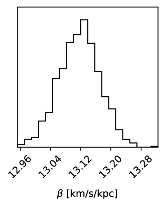
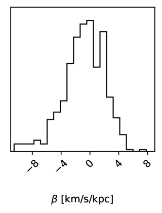
Figure 5: Corner plot of the Monte Carlo simulation using only data near the anticenter. Left: model of P20, with warp parameters of Chen et al. (2019). Right: model of Chrobáková et al. (2020).

4.4 Non-Gaussian Residuals of Least-squares Fit

In Figures 2, 3, and 4, we can see that the residuals of the least-squares fitting are not completely Gaussian, especially for the case of the warp model of Chrobáková et al. (2020) the residuals are skewed. To account for this effect, we performed one of the fits using Python’s method curve fit from the Scipy package. This fitting method has implemented several loss functions that we can apply to perform a more robust fit with less sensitivity to outliers. In Figure 6 we show the comparison of the fit using a linear loss function that corresponds to the standard least-squares fit with more robust loss functions such as Huber’s loss function and a smooth approximation of l1, which uses the sum of absolute deviations instead of squared ones (see Scipy documentation for more details). Change in the loss function influences the value of precession and the corresponding error, but compared to the error from the propagation of the warp parameters, this difference is insignificant; therefore, in all the cases we apply traditional least-squares as described in Section 3.

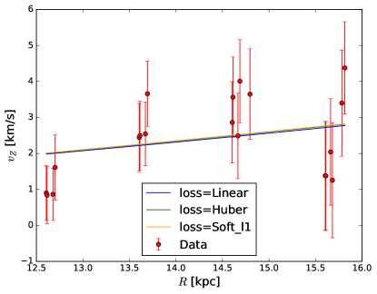
Figure 6: Comparison of the least-squares fit using different loss functions to treat outliers. We fit only data near the anticenter and we apply the warp model of Chrobáková et al. (2020). The linear loss function corresponds to the ordinary least-squares fit, where we obtain the value of precession $\beta=-1\pm 1.8$ km s^-1 kpc^-1. With a smooth approximation of l1 we obtain $\beta=-1.35\pm 2.21$ km s^-1 kpc^-1 and with Huber’s function we obtain $\beta=-1.07\pm 1.81$ km s^-1 kpc^-1. Note that in this case we only report the error of precession coming from the fit, not combined with the propagation of error of warp parameters, which is why the error is lower than in previous sections.

4.5 Comparison with Cheng et al. (2020)

The claims of P20 are supported in a recent paper of Cheng et al. (2020, hereafter C20), who used Gaia DR2 and APOGEE-2 DR16 to fit the warp from the kinematics. They use distances derived through Bayesian inference using the StarHorse code (Queiroz et al., 2018), which enables them to reach a high Galactocentric distance of $R=18$ kpc. They observe a significant decrease in vertical velocity, which they attribute to the warp. They adopt a model including the precession of warp and leave all the warp parameters free, except the line of nodes. They find a high amplitude of warp and a high value of warp precession of $\beta=13.57^{+0.20}_{-0.18}$ km s^-1 kpc^-1, similar to the value of P20. This is in disagreement with our results, due to the drop in the vertical velocity, beginning at about $R\approx 13$ kpc. We do not observe this in our data. As can be seen in Figure 7, our data show a decrease in vertical velocity, starting at about $R\approx 17$ kpc. We are aware that our statistical method to calculate the distance can give rise to errors; however, from the horizontal error bars in Figure 7 we can see that up to $R\approx 16$ kpc the data is robust and the error of the distance determination starts to be significant at higher distances. Therefore even taking into account the error bars, the drop in velocity would manifest itself at higher distances than given by C20.

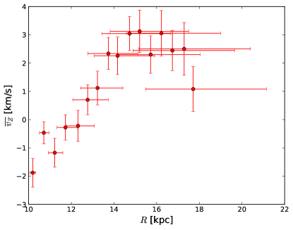
Figure 7: Average vertical velocity from Gaia DR2 including the complete range of azimuths. We do not observe a significant drop in velocity until $R\approx 17$ kpc. Due to large error bars, we constrain our analysis to $R<16$ kpc

As a further attempt to find the origin of the discrepancy in the data, we repeated the analysis carried out by C20 with similar data. C20 use two different datasets. One is a combination of Gaia DR2 with StarHorse distances. We are not aware that C20 put any constraints on these data, except filtering out stars that have a problematic Gaia photometric or astrometric solution or a troublesome StarHorse data reduction and removing stars from the Large Magellanic Cloud (LMC) and Small Magellanic Cloud (SMC). Therefore we have to assume they include all ranges of Galactic latitudes in this sample, thus not avoiding contamination by thick disk and halo stars. The second dataset of C20 combines Gaia DR2 with chemical and radial velocity information from APOGEE-2 DR16 and with StarHorse distances. C20 apply a constraint to this dataset in [Fe/H] and [Mg/Fe] in order to choose only thin disk stars (see their Figure 1). For both datasets, C20 observe a drop in velocities, although for the second sample the drop is less prominent. The first sample of C20 should be similar to what we are using, except we only chose stars with $\lvert b\rvert<$$$, which would explain the discrepancy. To reproduce the second sample, we used a publicly available dataset of Queiroz et al. (2020) who combined spectroscopic data from APOGEE-2 DR16 with photometric data and parallaxes from Gaia DR2 and distances derived using Starhorse. We applied the same selection criteria as C20 —we removed sources within $5\mathrm{°}$ from the center of LMC and SMC, we restricted the effective temperature between $3700$ K and $5500$ K, and we applied the same constraint in [Fe/H] and [Mg/Fe]. Our dataset is not exactly the same as the one of C20, but they should be in good agreement. However, upon applying the same conditions as C20, we do not observe a drop in velocities as C20 obtained. In fact, the velocity that we obtain is consistent with the velocity obtained when we applied our condition on the data, that is $\lvert b\rvert<$$$ (see Figure 8). Therefore we do not know what the reason is behind the drop in vertical velocity found by C20, but we suspect there might be contamination by the thick disk and the halo stars. In order to fit the warp, C20 used the Gaia sample that was not constrained and C20 state they assume this sample is not contaminated because the velocity has similar behavior to that of the thin disk in the Gaia-APOGEE sample. Although in principle this method of constraining the thin disk should be correct, we doubt that a full Gaia DR2 sample chosen within $\lvert b\rvert=$$$ has the same behavior of velocity as a strictly constrained thin disk sample of APOGEE. The fact that we cannot reproduce the drop in velocity at $R\approx 13$ kpc in either sample confirms this doubt, although we do not know with certainty what the reason is for this discrepancy.

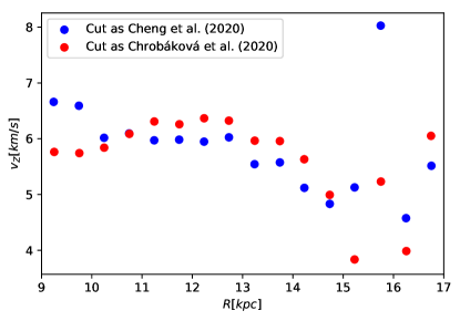
Figure 8: Average vertical velocity from Gaia DR2. For the blue curve we applied the same constraints as C20, most importantly a cut in [Fe/H] and [Mg/Fe] to choose only thin disk stars. For the red curve, we applied the same constraint as in our data, that is $\lvert b\rvert<$$$. Contrary to C20, we do not observe a significant drop in velocity for either approach.

C20 explain the drop in velocities solely in terms of warp and use only the vertical velocity to fit the warp parameters. We plot their warp amplitude in Figure 1, where we can see that their model yields far higher values than other works. We do not know if this result would be sustained by their stellar density, as C20 did not analyze the density distribution. However, Chrobáková et al. (2020) calculated warp parameters by fitting the stellar density and reaching a significantly lower warp amplitude.

Our argument is supported by other results in the literature as well, since most authors obtain far lower warp amplitude, between roughly $0.4-1$ kpc at $R=15$ kpc, depending on the stellar population and warp model (Yusifov, 2004; Reylé et al., 2009; Chen et al., 2019; Li et al., 2019; Skowron et al., 2019). The only work that supports the result of Cheng et al. (2020) is the one of Amôres et al. (2017), who produced star counts using a population synthesis model (Besançon Galaxy Model); therefore, we think their results should be interpreted with care since they are model-dependent.

5 Conclusions

We studied the precession of the Galactic warp based on the model of P20 and present our own calculation. We are using vertical velocities of Gaia DR2 that represent the average kinematics of an old stellar population ($\sim$5-6 Gyr) and we apply a new warp model (Chrobáková et al., 2020), based on Gaia DR2. Our warp model has a significantly smaller amplitude than models used by P20, which are either derived for a young stellar population ($\sim$Myr) or an invalid extrapolation of an old stellar population warp. When we consider variation of the amplitude of the warp with the age of the population, we obtain a best fit that is compatible with no precession, taking into account the uncertainties in a warp model independently derived from an old stellar density distribution with the same Gaia data. Therefore we do not find evidence to support or exclude any model of warp formation. Future studies are necessary to understand kinematics of warp and thus its formation mechanism. The next Gaia data release DR3 could provide sufficiently precise data, to study the warp in greater detail and possibly detect the precession.

References

- Ahumada et al. (2020) Ahumada, R., Allende Prieto, C., Almeida, A., et al. 2020, ApJS, 249, 3
- Amôres et al. (2017) Amôres, E. B., Robin, A. C., & Reylé, C. 2017, A&A, 602, A67
- Arenou et al. (2018) Arenou, F., Luri, X., Babusiaux, C., & et al. 2018, A&A, 616, A7
- Battaner et al. (1990) Battaner, E., Florido, E., & Sanchez-Saavedra, M. L. 1990, A&A, 236, 1
- Carney & Seitzer (1993) Carney, B. W. & Seitzer, P. 1993, AJ, 105, 2127
- Chen et al. (2019) Chen, X., Wang, S., Deng, L., et al. 2019, NatAs, 3, 320
- Cheng et al. (2020) Cheng, X., Anguiano, B., Majewski, S. R., et al. 2020, ApJ, 905, 49
- Chrobáková et al. (2020) Chrobáková, Ž., Nagy, R., & López-Corredoira, M. 2020, A&A, 637, A96
- Cropper et al. (2018) Cropper, M., Katz, D., Sartoretti, P., & et al. 2018, A&A, 616, A5
- Debattista & Sellwood (1999) Debattista, V. P. & Sellwood, J. A. 1999, ApJ, 513, L107
- Dubinski & Chakrabarty (2009) Dubinski, J. & Chakrabarty, D. 2009, ApJ, 703, 2068
- Gaia Collaboration et al. (2018) Gaia Collaboration, Brown, A. G. A., Vallenari, A., et al. 2018, A&A, 616, A1
- Gaia Collaboration et al. (2016) Gaia Collaboration, Prusti, T., de Bruijne, J. H. J., et al. 2016, A&A, 595, A1
- Jeon et al. (2009) Jeon, M., Kim, S. S., & Ann, H. B. 2009, ApJ, 696, 1899
- Jiang & Binney (1999) Jiang, I.-G. & Binney, J. 1999, MNRAS, 303, L7
- Karim & Mamajek (2017) Karim, M. T. & Mamajek, E. E. 2017, MNRAS, 465, 472
- Katz et al. (2019) Katz, D., Sartoretti, P., Cropper, M., & et al. 2019, A&A, 622, A205
- Kerr (1957) Kerr, F. J. 1957, AJ, 62, 93
- Kim et al. (2014) Kim, J. H., Peirani, S., Kim, S., et al. 2014, ApJ, 789, 90
- Li et al. (2019) Li, C., Zhao, G., Jia, Y., et al. 2019, ApJ, 871, 208
- Lindegren et al. (2018) Lindegren, L., Hernández, J., Bombrun, A., & et al. 2018, A&A, 616, A2
- López-Corredoira et al. (2014) López-Corredoira, M., Abedi, H., Garzón, F., & Figueras, F. 2014, A&A, 572, A101
- López-Corredoira et al. (2002a) López-Corredoira, M., Betancort-Rijo, J., & Beckman, J. E. 2002a, A&A, 386, 169
- López-Corredoira et al. (2002b) López-Corredoira, M., Cabrera-Lavers, A., Garzón, F., & Hammersley, P. L. 2002b, A&A, 394, 883
- López-Corredoira et al. (2020) López-Corredoira, M., Garzón, F., Wang, H. F., et al. 2020, A&A, 634, A66