Data-driven Langevin modeling of nonequilibrium processes

Abstract

Given nonstationary data from molecular dynamics simulations, a Markovian Langevin model is constructed that aims to reproduce the time evolution of the underlying process. While at equilibrium the free energy landscape is sampled, nonequilibrium processes can be associated with a biased energy landscape, which accounts for finite sampling effects and external driving. Extending the data-driven Langevin equation (dLE) approach [Phys. Rev. Lett. 115, 050602 (2015)] to the modeling of nonequilibrium processes, an efficient way to calculate multidimensional Langevin fields is outlined. The dLE is shown to correctly account for various nonequilibrium processes, including the enforced dissociation of sodium chloride in water, the pressure-jump induced nucleation of a liquid of hard spheres, and the conformational dynamics of a helical peptide sampled from nonstationary short trajectories.

I Introduction

Classical molecular dynamics (MD) simulations may account for the structure and dynamics of molecular systems in microscopic detail, but become cumbersome with increasing system size.Berendsen07 To drastically reduce the complexity, it is therefore often desirable to represent the considered process in terms of a small set of collective variables $\boldsymbol{x}=\{x_{i}\}$, also referred to as order parameters or reaction coordinates.Rohrdanz13 ; Peters16 ; Sittel18 Employing projection operator methods, Grabert80 ; Kubo85 ; Zwanzig01 in principle exact equations of motions for these variables, such as the generalized Langevin equation (GLE), can be derived. If we assume a time scale separation between the fast degrees of freedom (the bath) and the slow collective variables $\boldsymbol{x}$ (the system), we obtain a Markovian Langevin equation (LE)

$$m\ddot{\boldsymbol{x}}(t)=\boldsymbol{f}(\boldsymbol{x})-\Gamma(\boldsymbol{x})\dot{\boldsymbol{x}}(t)+\mathcal{K}(\boldsymbol{x})\boldsymbol{\xi}(t),$$ (1)

which describes the stochastic motion of a quasi-particle with mass $m$. Here the deterministic Newtonian force $\boldsymbol{f}=-\partial_{\boldsymbol{x}}\Delta G(\boldsymbol{x})$ is given by the gradient of the free energy landscape $\Delta G$, $\Gamma$ accounts for the friction tensor, $\mathcal{K}$ represents the diffusion tensor, and $\boldsymbol{\xi}(t)$ represents Gaussian-distributed white noise of zero mean. Friction and diffusion in general depend on variable $\boldsymbol{x}$ and are connected at thermal equilibrium by the fluctuation-dissipation theorem,Zwanzig01 $\mathcal{K}\mathcal{K}^{T}=2k_{\rm B}T\Gamma$.

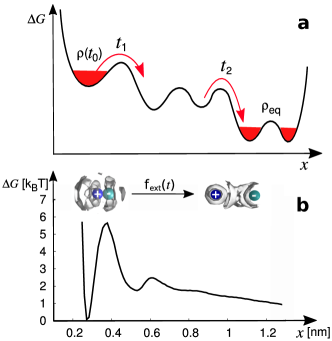
Figure 1: Nonequilibrium processes considered. (a) Relaxation: Starting in a nonstationary state $\rho(t_{0})$, the system evolves along the free energy landscape $\Delta G(x)$ towards its equilibrium state $\rho_{\rm eq}$. (b) External driving: Application of an external pulling force $f_{\rm ext}(t)$ along the interionic distance $x$ causes the dissociation of solvated NaCl along $\Delta G(x)$.

While Langevin theory is well established, Grabert80 ; Kubo85 ; Zwanzig01 a relatively little explored aspect concerns its application to nonequilibrium processes. For one, we may start in a nonstationary state $\rho(t_{0})$ (e.g., resulting from a laser-induced temperature-jump or photoexcitation) and study the relaxation of the (otherwise not driven) system into its equilibrium state $\rho_{\rm eq}$ (Fig. 1a). On the other hand, we may consider a system driven by an external force $f_{\rm ext}(t)$, as is the case, e.g., in atomic force microscopy experiments, where we mechanically pull a molecular complex apart (Fig. 1b). To account for such processes, the standard Langevin formalism can be generalized in various ways. Hernandez99 ; McPhie01 ; Micheletti08 ; Kawai11 ; Meyer17 ; Meyer19 ; Cui18 Using projection operator techniques, for example, several nonstationary versions of the GLE have been derived.Kawai11 ; Meyer17 ; Meyer19 Alternatively, we may consider a microscopic Hamiltonian of the full system, and derive equations of motion for the collective variables. Zwanzig73 This formulation can be readily extended to describe nonequilibrium relaxation processes by considering nonstationary initial conditions.Cui18 In the case of external driving, we expect that in the linear response regime the external force affects mainly the drift term $\boldsymbol{f}(\boldsymbol{x})$ but neither the friction $\Gamma$ nor the noise $\mathcal{K}$ of the LE.Cui18

Here we are concerned with the situation that we have nonstationary data $\boldsymbol{x}(t)$ (provided by an MD simulation or a time-dependent experiment) for which we want to construct a dynamical model that reproduces its time evolution. To this end, we need to determine the underlying parameters or fields of the model from the MD data.Straub87 ; Hummer05 ; Best06 ; Lange06b ; Hinczewski10 ; Perez-Villa18 ; Wolf18 ; Paul19 For example, when we employ the Markovian LE (1), we want to calculate the Langevin fields $\boldsymbol{f}$, $\Gamma$ and $\mathcal{K}$. To evaluate multidimensional Langevin fields from given MD data, we have developed a data-driven Langevin equation (dLE) approach, which was successfully applied to model the conformational dynamics of various peptides and proteins at equilibrium.Hegger09 ; Schaudinnus13 ; Schaudinnus15 ; Schaudinnus16 ; Lickert20

To extend the application of the dLE to the nonequilibrium regime, we derive the necessary modifications of the dLE algorithm for both relaxation and driven processes. In particular, we discuss the practical computation of nonstationary Langevin fields and discuss the dependence of these estimates on the sampling quality of the input data such as their length. As first applications, we demonstrate that the Markovian LE (1) correctly accounts for two nonequilibrium processes recently studied via a nonstationary GLE, Meyer17 ; Meyer19 that is, the enforced dissociation of NaCl in waterMeyer20 and the pressure-jump induced nucleation and growth process in a liquid of hard spheres.Meyer21 In both cases, a simple Langevin model is constructed that is shown to reproduce well the underlying MD reference data. As a Langevin-based enhanced sampling strategy,Rzepiela14 we finally consider the construction of a global Langevin model that accounts for the overall kinetics of the system, obtained from massive parallel computing of short MD trajectories that are per se nonstationary. Modeling the conformational dynamics of the helical peptide Aib₉ in five dimensions,Buchenberg15 we compare the predictions of the resulting dLE to a recently established Markov state model of the system.Biswas18

II Theory and Methods

II.1 Data-driven Langevin equation (dLE)

To briefly review the gist of the dLE approach,Hegger09 ; Schaudinnus13 ; Schaudinnus15 ; Schaudinnus16 ; Lickert20 we consider a discrete time series $\boldsymbol{x}_{n}\equiv\boldsymbol{x}(n\delta t)$ of the dimensionless coordinate $\boldsymbol{x}$ with time step $\delta t$. (For clarity, we henceforth use a vector notation.) By discretizing the time derivatives in Eq. (1), i.e, $\dot{\boldsymbol{x}}_{n}\rightarrow(\boldsymbol{x}_{n}-\boldsymbol{x}_{n-1})/{\delta t}$, we obtain a discrete version of the Langevin equationSchaudinnus15

$$\boldsymbol{x}_{n+1}=\boldsymbol{x}_{n}+\hat{\boldsymbol{f}}_{n}-\hat{\Gamma}_{n}(\boldsymbol{x}_{n}-\boldsymbol{x}_{n-1})+\hat{\mathcal{K}}_{n}\boldsymbol{\xi}_{n},$$ (2)

where we introduced the dLE fields

$$\hat{\boldsymbol{f}}_{n} =m^{-1}\delta t^{2}\boldsymbol{f}(\boldsymbol{x}_{n}), \hat{\Gamma}_{n} =m^{-1}\delta t\Gamma(\boldsymbol{x}_{n})-\mathbb{1},$$ (3)

$$\hat{\mathcal{K}}_{n} =m^{-1}\delta t^{3/2}\mathcal{K}(\boldsymbol{x}_{n}), \boldsymbol{\xi}_{n} =\boldsymbol{\xi}(\boldsymbol{x}_{n})\sqrt{\delta t},$$

accounting for drift $\hat{\boldsymbol{f}}(\boldsymbol{x})$, friction $\hat{\Gamma}(\boldsymbol{x})$ and noise amplitude $\hat{\mathcal{K}}(\boldsymbol{x})$ of the Langevin model.

Equation (2) can be used in two ways. In case that the dLE fields are given, it may be integrated to yield the time evolution of coordinate $\boldsymbol{x}_{n}$. On the other hand, if the time series $\boldsymbol{x}_{n}$ is given, we face the inverse problem and need to solve for the dLE fields defined by Eq. (3). Because of the stochastic nature of the noise $\boldsymbol{\xi}_{n}$, we can not determine these fields directly from the individual data points.Hegger09 Hence we introduce a local average of some observable $g(\boldsymbol{x})$

$$\langle g(\boldsymbol{x})\rangle=\frac{1}{k}\sum_{m}g(\boldsymbol{x}_{m}),$$ (4)

where the sum includes the $k$ nearest neighbors of reference point $\boldsymbol{x}$ which occur in the input time series. The neighborhood size $k$ needs to be small enough to allow for local (i.e., coordinate-dependent) averaging, but at the same time it should be large enough to achieve statistical convergence.Schaudinnus13 As a rule of thumb, a value of $k\approx 200$ performs well if $\gtrsim 10^{6}$ data points are available, and is therefore used in all cases below.

By exploiting the white noise properties $\langle\boldsymbol{\xi}_{n}\rangle=0$ and $\langle\boldsymbol{\xi}_{i}\boldsymbol{\xi}_{j}\rangle=\delta_{ij}$, we can derive from Eq. (2) explicit expressions for the dLE fieldsSchaudinnus15

$$\hat{\Gamma}_{n} =-C(\Delta\boldsymbol{x}_{n+1},\Delta\boldsymbol{x}_{n})C^{-1}(\Delta\boldsymbol{x}_{n},\Delta\boldsymbol{x}_{n}),$$ (5)

$$\hat{\boldsymbol{f}}_{n} =\langle\Delta\boldsymbol{x}_{n+1}\rangle+\hat{\Gamma}_{n}\langle\Delta\boldsymbol{x}_{n}\rangle,$$ (6)

$$\hat{\mathcal{K}}_{n}\hat{\mathcal{K}}^{T}_{n} =C(\Delta\boldsymbol{x}_{n+1},\Delta\boldsymbol{x}_{n+1})\!-\!\hat{\Gamma}_{n}C(\Delta\boldsymbol{x}_{n},\Delta\boldsymbol{x}_{n+1}),$$ (7)

where we introduced the displacement $\Delta\boldsymbol{x}_{n}\!=\!\boldsymbol{x}_{n}\!-\!\boldsymbol{x}_{n-1}$ and the covariance $C(\boldsymbol{x},\boldsymbol{y})=\langle\boldsymbol{x}\boldsymbol{y}^{T}\rangle-\langle\boldsymbol{x}\rangle\langle\boldsymbol{y}^{T}\rangle$, with averages as in Eq. (4). In a last step, a Cholesky decomposition of $\hat{\mathcal{K}}_{n}\hat{\mathcal{K}}^{T}_{n}$ is used to calculate the noise amplitude matrix $\hat{\mathcal{K}}_{n}$.Schaudinnus13 Equations (2) – (7) constitute the working equations of the dLE. That is, by calculating dLE fields $\hat{\boldsymbol{f}}_{n}$, $\hat{\Gamma}_{n}$ and $\hat{\mathcal{K}}_{n}$ from the input data $\boldsymbol{x}_{n}$, we propagate Eq. (2) to obtain a dLE trajectory, which then can be employed to predict statistical and dynamical properties of the system.

Since the dLE is based on a Markovian approximation, it requires a propagation time step $\delta t$ that is longer than the memory time of the system, while $\delta t$ simultaneously needs to be short enough to resolve the dynamics of the system. Choosing $\delta t$ to meet the second condition, we may test the validity of the resulting dLE model by imagining that the input trajectory $\boldsymbol{x}_{n}$ was generated by the propagation of Eq. (2). Analyzing the properties of the resulting noise trajectory

$$\boldsymbol{\xi}_{n}=\hat{\mathcal{K}}_{n}^{-1}(\boldsymbol{x}_{n+1}-\boldsymbol{x}_{n}-\hat{\boldsymbol{f}}_{n}+\hat{\Gamma}_{n}(\boldsymbol{x}_{n}-\boldsymbol{x}_{n-1})),$$ (8)

we can check if the noise indeed fulfills the criteria of white noise such as zero mean and $\delta$-correlation. Schaudinnus13 Failing this test indicates that the time step is too short for the presumed Markov approximation of the dLE model. As a remedy, we recently proposed to rescale the friction and the noise tensor of the dLE via $\Gamma\rightarrow S\Gamma S^{T}$ and $\mathcal{K}\rightarrow S\mathcal{K}$, in order to obtain the correct long-time behavior of the system.Lickert20 To determine the scaling factor $S$, we require that the resulting dLE model reproduces the correct initial decay of the position autocorrelation function.

To facilitate the treatment of multidimensional systems, the dLE fields are calculated “on the fly”, i.e., at every propagation step of the dLE trajectory.Hegger09 The drawback of this strategy is that the local averaging in Eq. (4) requires the determination of the $k$ nearest neighbors of all $N$ data points at every dLE step. Besides using an efficient box-assisted search Grassberger90 (which scales $\propto N\ln N$), we recently introduced a “pre-averaging” approach which exploits the fact that the dLE fields are estimated from local neighborhoods, and allows for a massive reduction of data points (say, from $10^{7}$ input points to $10^{5}$ averaged points) that need to be scanned in every dLE step (see SI methods for details).Lickert20

Let us finally note two features of the dLE that are particularly valuable for its application to general nonequilibrium processes. First off, the calculation of dLE fields in Eqs. (2) – (7) in principle requires only short trajectory pieces (i.e., at least three successive time steps). This local information does not require global equilibrium data, but can be readily obtained from short nonstationary data.Rzepiela14 Secondly, we note that the dLE of time series $\boldsymbol{x}(t)$ in Eq. (2) does not involve the mass tensor $m$, because it is included in the definition of the dLE fields. Hence, we are not restricted to the modeling of the motion of particles, but can use Eq. (2) to model the stochastic time evolution of an arbitrary phase-space function $\boldsymbol{A}(t)$.

II.2 dLE modeling of relaxation processes

To apply the dLE formulation to nonstationary data, we first focus on the case shown in Fig. 1a, where the system is prepared at time $t_{0}\!=\!0$ in a nonstationary state $\rho(t_{0})$ and for $t\!>\!t_{0}$ relaxes towards its equilibrium state $\rho_{\rm eq}$. While the initial state of the process is by design nonstationary, the definition of the system (e.g., via a microscopic system-bath Hamiltonian or an MD force field) is the same as for an equilibrium process and therefore associated with the free energy landscape $\Delta G(\boldsymbol{x})$. Since the Langevin fields $\boldsymbol{f}$, $\Gamma$ and $\mathcal{K}$ derive from this Hamiltonian,Zwanzig01 they should be the same as well. In principle we can therefore again construct an appropriate Langevin model from a long equilibrium trajectory, and use local averages [Eq. (4)] to calculate the dLE fields $\hat{\boldsymbol{f}}_{n}$, $\hat{\Gamma}_{n}$ and $\hat{\mathcal{K}}_{n}$.

In practice, though, equilibrium MD data would hardly sample the initial high-energy regions of the process (Fig. 1a), which are of interest when we study the time evolution of the relaxation. Similar to experiment, we therefore perform an ensemble average over numerous nonequilibrium trajectories $\boldsymbol{x}^{(r)}(t_{n})\equiv\boldsymbol{x}_{n}^{(r)}$ ($r=1,\ldots,N_{\rm traj}$) of some length $t_{\rm max}$, and calculate local averages of the dLE fields from this data. As a consequence, the accuracy of the dLE field estimation will depend on the sampling parameters $N_{\rm traj}$ and $t_{\rm max}$. For example, in the case of a short trajectory length $t_{\rm max}$, the model may only account for the initial dynamics at times $t\lesssim t_{1}$, but can not describe its further relaxation to equilibrium for $t\gtrsim t_{2}$ (Fig. 1a).

To discuss the effects of a finite sampling time $t_{\rm max}$, we consider the resulting drift field of the dLE, given by $\boldsymbol{f}(\boldsymbol{x})=-\partial_{\boldsymbol{x}}\Delta G(\boldsymbol{x})$. At equilibrium, $\Delta G(\boldsymbol{x})$ represents the free energy landscape, $\Delta G(\boldsymbol{x})=-k_{\rm B}T\ln P(\boldsymbol{x})$ with equilibrium distribution $P(\boldsymbol{x})$. When we estimate the potential from $N_{\rm traj}$ nonequilibrium trajectories of length $t_{\rm max}$, we correspondingly obtain a “biased energy landscape” Post19 $\Delta{\cal G}(\boldsymbol{x})$ that depends on the distribution ${\cal P}(\boldsymbol{x})\propto\int dt\rho(\boldsymbol{x},t)$ sampled within $0\leq t\leq t_{\rm max}$,

$$\Delta{\cal G}(\boldsymbol{x})=-k_{\rm B}T\ln{\cal P}(\boldsymbol{x}),$$ (9)

and approaches the equilibrium free energy landscape only for $t_{\rm max}\!\rightarrow\!\infty$. Limited sampling in particular means that $\Delta{\cal G}(\boldsymbol{x})$ may not cover all parts of the equilibrium energy landscape $\Delta G(\boldsymbol{x})$, see Sec. III.1. Note that the term “biased” here refers to the nonstationary initial conditions, and should not be confused with biased potentials in enhanced sampling techniques.Berendsen07

We note that both, $\Delta G(\boldsymbol{x})$ and $\Delta{\cal G}(\boldsymbol{x})$, represent a global observable of the system. The drift field $\boldsymbol{f}\!=\!-\partial_{\boldsymbol{x}}\Delta{\cal G}$, on the other hand, measures the slope of the energy landscape at position $\boldsymbol{x}$. It can be therefore estimated by the local average in Eq. (4) via a sum over the $k$ nearest neighbors of $\boldsymbol{x}$. Because the dLE fields are generally based on local averages, the same argument hold also for the friction $\hat{\Gamma}_{n}\equiv\hat{\Gamma}(\boldsymbol{x}(t_{n}))$ [Eq. (5)] and the noise $\hat{\mathcal{K}}_{n}\equiv\hat{\mathcal{K}}(\boldsymbol{x}(t_{n}))$ [Eq. (7)].

To construct a dLE model of nonequilibrium relaxation, we therefore (i) calculate the dLE fields for the given nonstationary data and (ii) perform dLE runs using initial conditions of the relaxation process. While no additional assumptions are involved (compared to an equilibrium dLE), the nonstationary dLE model depends on the sampling achieved by the input data, in particular on their length (see Sec. III.1).

II.3 dLE modeling of external driving

Unlike to the modeling of relaxation processes, where the dLE fields are in principle the same as at equilibrium, external driving via some force $\boldsymbol{f}_{\rm ext}(\boldsymbol{x},t)$ will change these fields. First of all, the deterministic drift term $\boldsymbol{f}(\boldsymbol{x})$ in Eq. (2) needs to be complemented by the external perturbation $\boldsymbol{f}_{\rm ext}(\boldsymbol{x},t)$. In a microscopic description, such as an all-atom MD simulation, this is all to be done - external forces can simply be added to the internal forces. In a reduced description such as a Langevin model, however, external forces may in principle also affect the friction $\Gamma$ and the noise $\mathcal{K}$ of the model.Meyer17 ; Meyer19 ; Daldrop17 In the linear-response regime, we nevertheless expect that nonequilibrium and equilibrium dynamics exhibit the same friction and noise. According to Onsager’s regression hypothesis,Chandler87 this is because in this regime nonequilibrium perturbations are governed by the same laws as equilibrium fluctuations. For example, when we derive LE (1) from a system-bath ansatz where a general system is linearly coupled to a harmonic bath,Zwanzig73 we find that external and internal forces are simply added.Cui18

Given a dLE model constructed from equilibrium data and an external potential $V_{\rm ext}(\boldsymbol{x},t)$ that affects a linear response of the system, we thus obtain a dLE for the driven nonequilibrium processes by replacing the free energy landscape $\Delta G(\boldsymbol{x})$ of the equilibrium model by the biased energy landscape

$$\Delta{\cal G}(\boldsymbol{x},t)=\Delta G(\boldsymbol{x})+V_{\rm ext}(\boldsymbol{x},t).$$ (10)

As a simple example, we consider an atomic force microscopy experiment that causes the dissociation of a diatomic molecule (Fig. 1b). The one-dimensional pulling can be modeled via a harmonic spring, Grubmueller96 ; Isralewitz01 ; Park04

$$V_{\rm ext}(x,t)=-\frac{C}{2}[x(t)-(x_{0}+vt)]^{2},$$ (11)

where $C$ is the spring constant and $v$ the pulling velocity. As a consequence, the system is gradually pulled along the free energy landscape $\Delta G(x)$ in Fig. 1b. That is, the biased energy landscape $\Delta{\cal G}$ corresponds to the total deterministic potential experienced by the system at time $t$. This simple picture is expected to be valid for most biomolecular applications taking place close to equilibrium. Considering the enforced dissociation of NaCl discussed below, for example, we found linear response behavior for pulling velocities up to $\sim 10\,$ m/s, at which the pulling approaches the picosecond timescale of the reordering of the solvation shells.Wolf18

To go beyond the linear response or to construct a dLE directly from data of a driven system, we need to calculate explicitly time-dependent dLE fields from the nonequilibrium data. Hence the local average of function $g(\boldsymbol{x})$ in Eq. (4) has to be replaced by a time-dependent average $\langle g(\boldsymbol{x},t)\rangle$. Assuming that the nonequilibrium process is sampled by $N_{\rm traj}$ trajectories $\boldsymbol{x}_{n}^{(r)},$ this ensemble average can be written as

$$\langle g(\boldsymbol{x},t_{n})\rangle=\frac{1}{N_{\rm traj}}\sum_{r=1}^{N_{\rm traj}}g(\boldsymbol{x}_{n}^{(r)})\,\delta_{k}(\boldsymbol{x}-\boldsymbol{x}_{n}^{(r)}),$$ (12)

where $\delta_{k}(\boldsymbol{x}-\boldsymbol{x}_{n}^{(r)})$ defines a boxing function that is equal to $1/k$ for the $k$ nearest neighbors of $\boldsymbol{x}$ and zero otherwise.

II.4 Comparison to the nonstationary GLE

The Markovian LE (1) is based on a time scale separation between the fast bath degrees of freedom and the slow collective variable $\boldsymbol{x}$. On the other hand, various generalized LEs (GLEs) have been proposed that are not limited to a Markov-type approximation. To describe nonequilibrium processes, in particular, Schilling and coworkers recently employed a time-dependent projection operator formalism to derive for some variable $A(t)$ the nonstationary GLE Meyer17 ; Meyer19

$$\dot{A}(t)=\omega(t)A(t)+\int_{0}^{t}d\tau K(t,\tau)A(\tau)+\eta(t),$$ (13)

where memory kernel $K$ and noise $\eta$ are related by a generalized fluctuation-dissipation theorem. Due to the Mori-type projection employed, the equation exhibits a linear drift term $\omega(t)A(t)$ that vanishes for a mean-free variable $A(t)$.

It is instructive to compare this formulation to our Markovian Langevin approach, also because we adopt below two model problemsMeyer20 ; Meyer21 that were previously studied with this GLE. In these studies, the GLE analysis resulted in slowly decaying memory kernels, which appears to question the applicability of a Markovian Langevin model such as the dLE. However, whether a timescale separation is given depends on the system-bath partitioning of the problem. As we show in the following, the LE (1) and the GLE (13) are based on different partitionings, where the former may be valid, although the latter exhibits non-Markovian behavior.

Following Zwanzig,Zwanzig01 we explain this difference for the case of a one-dimensional system variable $x(t)$. To begin, we rewrite the second-order differential equation (1) for $x(t)$ in terms of two first-order equations,

$$\dot{x}(t) = p(t)/m,$$ (14)

$$\dot{p}(t) = f(x)-\Gamma p(t)+\mathcal{K}\xi(t),$$ (15)

for the phase space variables $x(t)$ and $p(t)$. Integrating Eq. (15), we obtain

$$\begin{split}p(t)=&\int_{0}^{t}\mathrm{d}\tau\,{\mathrm{e}}^{-\Gamma(t-\tau)/m}f(x(\tau))\\ &+\int_{0}^{t}\mathrm{d}\tau\,{\mathrm{e}}^{-\Gamma(t-\tau)/m}\mathcal{K}\xi(\tau),\end{split}$$ (16)

where we assumed that $p(0)\!=\!0$. Insertion in Eq. (14) yields the desired GLE for $x(t)$,

$$\dot{x}(t)=\int_{0}^{t}\mathrm{d}\tau K(t,\tau)x(\tau)+\eta(t).$$ (17)

It contains a two-time memory kernel

$$K(t,\tau)=\frac{1}{m}\,{\mathrm{e}}^{-\Gamma(t-\tau)/m}\,\frac{f(x(\tau))}{x(\tau)},$$ (18)

which in the case of a linear force (${f(x(\tau))}/{x(\tau)}\!=$const.) reduces to a simple exponential function that depends only on the time difference $t\!-\!\tau$. The function $\eta(t)$ represents the corresponding colored noise. Note that the GLE (17) for $x(t)$ is equivalent to the Markovian LEs (14) and (15) for $x(t)$ and $p(t)$, that is, both formulations describe the same physics. Non-Markovian features of the GLE such as a slowly decaying memory kernel (18) may therefore reflect a slowly varying force, which arises from a multistate energy landscape with rarely occurring transitions.

Because Eq. (17) is of similar form as the nonstationary GLE (13), the above argument holds also in this case. Nonetheless, the nonstationary GLE represents an exact formulation,Meyer17 ; Meyer19 that is, for any nonequilibrium process a GLE (13) can be defined via the functions $\omega(t)$, $K(t,\tau)$ and $\eta(t)$ that do not depend on coordinate $x$. Employing the dLE, on the other hand, we need to assume that a Markovian LE model exists for the considered process. As a trade-off we obtain a physically intuitive model, where the biased energy landscape $\Delta{\cal G}$ accounts for the main features of the considered process, and the friction $\Gamma$ and the noise $\mathcal{K}$ describe in a transparent way the effects of the bath.

III Results and discussion

III.1 Hierarchical energy landscape

We begin with the first nonequilibrium scenario where the system is initially prepared in a nonstationary state and subsequently relaxes into its equilibrium state (Fig. 1a). As discussed in Sec. II.2, the dLE modeling of nonequilibrium relaxation processes may sensitively depend on the length $t_{\rm max}$ of the input data. This is particularly true for biomolecular systems that are characterized by a hierarchical energy landscape, which gives rise to coupled processes on timescales ranging from, say pico- to milliseconds. Frauenfelder91 ; Henzler-Wildman07 ; Buchenberg15 To demonstrate the effect of finite data length on a dLE model, we consider a one-dimensional free energy landscape with three consecutive energy barriers of similar height, see Fig. 2. The model aims to mimic photo- or ligand-induced conformational transitions in proteins,Buchenberg17 ; Bozovic20 where at time $t\!=\!0$ the system is prepared in the nonstationary state 1, evolves via intermediate states 2 and 3, and finally reaches the second low-energy state 4. Due to the hierarchical shape of the free energy landscape, transition 1$\rightarrow$2 occurs much more rapidly than transition 1$\rightarrow$3 or even 1$\rightarrow$4, because the latter require the previous transitions as a prerequisite step.

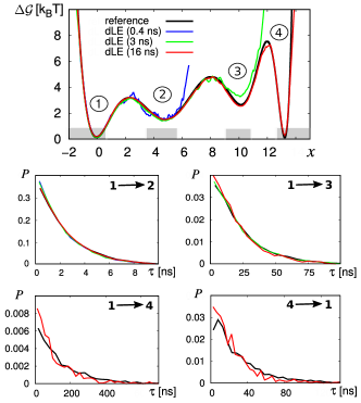
Figure 2: (Top) Hierarchical free energy landscape (black), which consists of states ${\bf 1}-{\bf 4}$ connected via energy barriers of similar height. Gray regions at the bottom define cores of the states used to calculate waiting times. Starting in state 1, sets of trajectories of lengths $t_{\rm max}=0.4\,$ns, 3 ns, and 16 ns are generated, which result in nonequilibrium energy landscapes $\Delta{\cal G}(x)$ [Eq. (9)] reaching state 2 (blue), 3 (green), and 4 (red), respectively. (Bottom) Distributions of waiting times $\tau_{i\rightarrow j}$ of transitions i$\rightarrow$j as indicated. Results from dLE models using input data of length 0.4 ns (blue), 3 ns (green), and 16 ns (red) are compared to reference data (black).

Using this energy landscape, a mass of $m=26\,$u, constant friction ($\Gamma\!=\!130\,$kJ ps/(mol nm²)) and noise amplitude ($\mathcal{K}\!=\!25\,$kJ ps^1/2/(mol nm)), a temperature $T=300\,$K, and a time step $\delta t=0.04$ ps, we run $20\!\times\!16\,\mu$s-long Langevin trajectories as reference data, each trajectory starting at $x=0$. Here we are interested in the waiting times of transitions between states $i$ and $j$,Gernert14 i.e., the time spend in state $i$ and possible subsequent intermediate states before going to state $j$. Figure 2 shows the resulting waiting time distributions, Table 1 lists the corresponding mean values $\tau_{i\rightarrow j}$. We find that $\tau_{1\rightarrow 2}\!=\!2.5\,$ns is about one order of magnitude shorter than $\tau_{1\rightarrow 3}\!=\!23\,$ns, which again is almost an order of magnitude shorter than $\tau_{1\rightarrow 4}\!=\!143\,$ns. Back transitions from states 2, 3 and 4 to state 1 occur with waiting times of $2.4\,$ns, $8\,$ns, $30\,$ns, respectively. The resulting nonequilibrium energy landscape $\Delta{\cal G}(x)$ [Eq. (9)] is indistinguishable from the (analytically given) free energy landscape in Fig. 2.

Employing these simulation results as input data, we now construct a dLE of the hierarchical dynamics. Since the dLE is by design clearly suited to reproduce data obtained by a Markovian LE, we can focus on the effect of limited input data length $t_{\rm max}$ on the resulting model. Guided by the waiting time distributions shown in Fig. 2, we construct three input data sets consisting of $10^{2}$ LE trajectories each starting in state 1 with $t_{\rm max}=0.4\,$ns, 3 ns, and 16 ns. These times are just long enough to catch about ten transitions from state 1 to state 2, 3 and 4, respectively. Using a time step of $\delta t\!=\!0.04$ ps and a pre-averaging of the input data sets to $10^{4}$ points (see SI Methods), we run for each input data set $10\!\times\!10\,\mu$s-long dLE simulations, which means that we sample the different transitions at least $10^{3}$ times. The effect of the finite input data length is clearly shown by the resulting dLE nonequilibrium energy landscapes $\Delta{\cal G}(x)$ which, depending on the chosen value for $t_{\rm max}$, cover the first two, three or all four states (see Fig. 2). In a similar way, the dLE reproduces the friction $\Gamma(x)\!=\,$const. and the noise amplitude $\mathcal{K}(x)\!=\,$const. of the model (Fig. S1).

Considering transition 1$\rightarrow$2, we find that a dLE constructed from $0.4\,$ns-long data predicts a mean waiting time $\tau_{1\rightarrow 2}\!=\!2.4\,$ns that is about 4% shorter than the reference (Tab. 1). The corresponding distribution in Fig. 2 reveals that this effect is mainly caused by an overestimation of fast transitions. Increasing the input data length, distribution and mean value converge to the reference data. Similar results are also found for the 1$\rightarrow$3 transition. Transitions involving the low-energy state 4 show somewhat larger deviations. Using input data of 16 ns length, the waiting times for the 1$\leftrightarrow$4 transition are underestimated by about 20 %. Again we find that short input data bias towards short waiting times.

data	$\tau_{\text{1}\rightarrow\text{2}}$	$\tau_{\text{1}\rightarrow\text{3}}$	$\tau_{\text{1}\rightarrow\text{4}}$	$\tau_{\text{4}\rightarrow\text{1}}$
reference	$2.5\pm 0.01$	$23\pm 0.2$	$143\pm 3.3$	$30\pm 0.7$
dLE (0.4 ns)	$2.4\pm 0.02$	–	–	–
dLE (3 ns)	$2.4\pm 0.01$	$22\pm 0.3$	–	–
dLE (16 ns)	$2.5\pm 0.02$	$21\pm 0.3$	$110\pm 4.3$	$24\pm 0.9$

Table 1: Average waiting times (in ns) of the transitions $i\rightarrow j$ of the hierarchical energy landscape in Fig. 2, obtained for the reference data and for dLE models with different length $t_{\rm max}$ of the input data (given in parenthesis). Errors are calculated as standard deviations of the mean.

To summarize, while the input data for a dLE model obviously need to be long enough to reach a specific conformational state at all, it is noteworthy that only a few events are sufficient for the dLE to qualitatively predict the waiting times to these state.

III.2 Enforced ion dissociation of NaCl in water

As an example of an externally driven process, we now consider the dissociation of solvated sodium chloride, which has served as a versatile model problem to test the validity of various Langevin formulations. This includes a dLE model constructed from equilibrium MD data, Lickert20 a Markovian LE obtained from dissipation-corrected targeted MD calculations of the free energy and the friction,Wolf20 and the nonstationary GLE constructed from pulling simulations. Meyer20 Here we adopt pulling simulations of NaCl along the interionic distance $x$ with pulling velocity $v\!\!=\!\!10\,$m/s, using the external force in Eq. (12) and an ensemble average over 1000 nonequilibrium trajectories.Meyer20 This MD data serve as a reference to study the applicability of a Markovian Langevin description of this problem. As detailed in Ref. Wolf18, , all MD simulations employed Gromacs v2018 (Ref. Abraham15, ) in a CPU/GPU hybrid implementation, using the Amber99SB* force fieldHornak06 ; Best09 and the TIP3P water model.Jorgensen83

To illustrate the dissociation process, Fig. 1b shows the free energy profile of NaCl along its interionic distance $x$, whose main maximum at $x\approx 0.4$ nm corresponds to the binding-unbinding transition of the two ions. The second smaller maximum at $x\approx 0.6$ nm reflects the transition from a common to two separate hydration shells.Mullen14 Pulling NaCl apart using a strong ($C\!=\!1000\,$ kJ/(mol nm²)) and a soft ($C\!=\!100\,$ kJ/(mol nm²)) spring, we obtain representative trajectories $x(t)$ as shown in Figs. 3a,c, respectively. For a strong spring, the system remains in the bound state for $t\lesssim 20$ ps, before it abruptly moves over the main barrier to the unbound state, where the Na-Cl distance $x(t)$ grows linearly with time. The transition time of the individual trajectories exhibits a narrow distribution with a width of the order of 10 ps. In the weak spring simulations, on the other hand, the transition time distribution is rather broad, such that the individual trajectories seem to cross the barrier at random times.

To account for the statistical properties of the nonstationary time series $x(t)$, we introduce the mean-free variable Meyer20

$$\delta x(t)=\frac{x(t)-\langle x(t)\rangle}{\langle(x(t)-\langle x(t)\rangle)^{2}\rangle^{1/2}}\,,$$ (19)

which removes the systematic drift due to the pulling. The autocorrelation function of this variable at time $t$,

$$C_{x}(t,t\!+\!\tau)=\langle\delta x(t)\delta x(t\!+\!\tau)\rangle$$ (20)

drawn with respect to the delay time $\tau$ is shown in Figs. 3e,g for strong and soft springs, respectively. In the former case, the autocorrelation decays on a timescale of 1 ps, except when the system is at the barrier ($t=10-15$ ps), where the decay is significantly slower ($\sim 5$ ps). While the fast decay of 1 ps can be associated with hydration shell dynamics around the ions (which drives the ion dissociation), Wolf18 the slow decay is caused by forward- and backward crossing events over the main free energy barrier of the system. For a weak spring, $C_{x}$ generally decays slower ($\sim 20$ ps) for all times $t$.

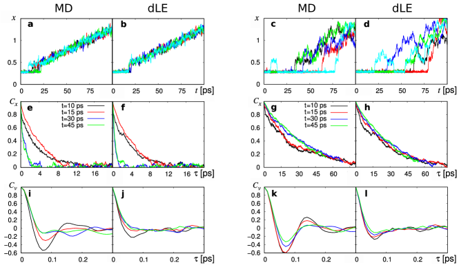
Figure 3: Enforced dissociation of solvated NaCl. Comparing results from reference MD simulations and dLE model, we show (top) five sample trajectories, (middle) the position autocorrelation function $C_{x}$, and (bottom) the velocity autocorrelation function $C_{v}$, obtained for a strong spring (left) and a weak spring (right).

We now turn to the Langevin modeling of the enforced dissociation of NaCl. To this end, we adopt a previously describedLickert20 dLE model constructed from equilibrium data at $300\,$K, which reproduces the MD dissociation time (130 ps) and association time (850 ps) within an error of a few percent. The model uses a sufficiently short propagation time step to resolve the dynamics ($\delta t\!=\!10\,$fs), the reduced mass of NaCl ($m\!=\!13.88$ u), a drift field corresponding to the free energy profile shown in Fig. 1b, and constant friction ($\Gamma\!=\!594\,$kJ ps/(mol nm²)) and noise amplitude (${\cal K}\!=\!54\,$kJ ps^1/2/(mol nm)). Adding the pulling force [Eq. (12)] to this dLE model, we wish to investigate to what extent the resulting Langevin description can account for the MD reference results.

By comparing the Langevin trajectories to the corresponding MD results, Figs. 3a-d reveal that the Markovian LE mimics the MD data quite closely. The same holds for the the position autocorrelation function $C(t,t\!-\!\tau)$, which is reproduced in excellent agreement (Figs. 3e-h). This means that –at least for the cases considered– the enforced dissociation of NaCl can be well described by a Markovian Langevin model. Since we simply added an external force to an equilibrium dLE model, we have shown that the external driving does not affect the validity of the friction and the noise estimated at equilibrium conditions. Alternatively, we could estimate the Langevin fields directly from the nonequilibrium data, which is advantageous when dissipation-corrected targeted MD simulations are available.Wolf20

To demonstrate the limits of the Markovian approximation underlying the dLE, we consider the velocity autocorrelation function $C_{v}$ shown in Figs. 3i-l. It exhibits a rapid initial decay on a $\sim 25\,$fs timescale, which is followed by damped oscillatory features with a period of $\sim 120\,$fs, whose details depend on time $t$ (see Ref. Meyer20, ). Similar as found for the equilibrium dLE model,Lickert20 the Markovian LE correctly obtains the initial decay of $C_{v}$, but underestimates the oscillations. While the Markovian Langevin model fails to catch these details on short timescales ($t\lesssim 0.1\,$ps), it reproduces correctly the equilibrium and nonequilibrium ion dynamics on timescales of 1 – 1000 ps.

III.3 Pressure-induced crystal nucleation of hard spheres

As a potentially more challenging example, we next consider crystal nucleation and growth processes in a compressed liquid of hard spheres, which was recently studied as a test problem for the nonstationary GLE.Kuhnhold19 ; Meyer21 Adopting 16384 hard spheres with mass $m$ and diameter $\sigma$ and using a time step $\delta t\!=\!\sqrt{m/(k_{\text{B}}T)}\sigma$, Meyer et al.Meyer21 first equilibrated the system in a liquid state at a volume fraction $\eta_{0}\!=\!0.45$. At time $t\!=\!0$ crystallization is induced by impulsively compressing the system to a volume fraction $\eta\!=\!0.54$ by rescaling the simulation box and all positions, and $N_{\rm traj}\!=\!580$ trajectories of $t_{\rm max}\!=\!214\,\delta t$ length were propagated. Using these nonequilibrium trajectories as input data for a dLE, here we want to study to what extent a Markovian Langevin model is able to describe the complex cooperative processes underlying this weak first-order phase transition.tenWolde95

As a one-dimensional reaction coordinate that accounts for the crystallinity of the system, we choose the percentage $x$ of particles that completed crystallization, which is readily calculated from the $Q_{6}$ order parameter.Meyer21 ; tenWolde95 To get an overview of the nucleation dynamics of the system, Fig. 4a shows the time evolution $x(t)$ of eight sample trajectories. Due to the mandatory preceding formation of nucleation seeds, the crystallization process starts after some induction time, which is widely distributed. The subsequent nucleation process is reflected in a rapid sigmoidal-shaped rise of $x(t)$ on a timescale of $20\,\delta t$. The majority (357) of the trajectories rises to a value of $x\!\gtrsim\!0.8$ where they level off and slowly approach the limiting value $x\!=\!1$. A smaller part (125) gets stuck at a value of $x\!\sim\!0.65$, reflecting the occurrence of crystal defects. Meyer21 ; tenWolde95 The remaining trajectories start too late to reach one of the two plateaus. Averaging over all trajectories (Fig. 4c), the nucleation process is found to occur on a timescale of $100$ $\delta t$.

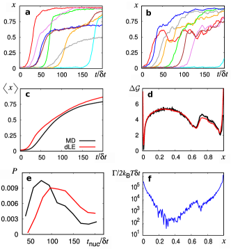
Figure 4: Pressure-induced crystal nucleation of hard spheres, indicated by the percentage $x$ of particles that completed crystallization. Representative trajectories $x(t)$ obtained from (a) reference MD and (b) corresponding dLE simulations. Comparing MD and dLE results, shown are (c) the average percentage $\langle x(t)\rangle$, (d) the resulting energy landscape $\Delta{\cal G}(x)$, and (e) the distribution of nucleation times $t_{\rm nuc}$. Panel (f) shows the friction coefficient $\Gamma(x)$ estimated by the dLE.

Figure 4d shows the corresponding nonequilibrium energy landscape $\Delta{\cal G}(x)$ defined in Eq. (9). Here the minimum at $x\!\sim\!0.014$ reflects the initial liquid state of the system, and the minimum at $x\!\sim\!0.65$ accounts for the defective clusters. The minimum at $x\!\sim\!0.95$ corresponds to (almost) completed crystals, and depends sensitively on the finite length $t_{\rm max}$ of the nonequilibrium trajectories. Increasing $t_{\rm max}$, more and more trajectories reach the crystalline end state, which leads to a steep decrease of the energy for $x\!\rightarrow\!1$. To define a nucleation time $t_{\rm nuc}$, we choose $x\!=\!0.8$ as a threshold value for the nucleation. Figure 4d shows the resulting distribution of $t_{\rm nuc}$. Due to the relatively small sample size (only 357 trajectories reach $x\!=\!0.8$), the distribution is given at low resolution. It peaks at $t_{\rm nuc}=76\,\delta t$ and yields a mean nucleation time of $102\,\delta t$.

To construct a dLE model of the nonequilibrium MD data, we first employ the noise test of Eq. (8) to verify that a dLE using the data time step $\delta t$ results in a correct model of white noise (see Fig. S2). Then $10^{4}$ dLE trajectories of length $t_{\rm max}\!=\!214\,\delta t$ were simulated, each run starting at $x=0.02$. Comparing the individual trajectories of MD and dLE (Figs. 4a,b) as well as their averages (Fig. 4c), we find that the dLE qualitatively reproduces the induction time distribution and the sigmoidal-shaped rise of $x(t)$. Moreover, the resulting nonequilibrium energy landscape $\Delta{\cal G}(x)$ shown in Fig. 4d is found to be in excellent agreement with the MD results. Unlike to the MD results, though, the dLE trajectories mostly do not directly rise to $x\!\gtrsim\!0.8$, but stay for some time around $x\sim 0.65$ before they rise further. This deviation is a consequence of the local estimation of the dLE fields [Eq. (4)], which does not distinguish between crystallizing and defective trajectories. As a consequence the resulting dLE distribution of nucleation times $t_{\rm nuc}$ in Fig. 4e is somewhat shifted compared to the MD distribution, which results in a mean dLE nucleation time of $128\,\delta t$ (rather than $102\,\delta t$). Due to the limited statistics of the MD data, though, this discrepancy might change for better sampled data. For longer MD trajectories, for example, we expect also longer nucleation times, since gradually all non-defective trajectories crystallize.

Let us finally study the friction $\Gamma$ as a function of variable $x$. Figure 4f shows that the friction is low at the main barrier and high at the two main minima reflecting the liquid and crystallized state. In line with previous results,Wolf20 we find that the friction rises in particular at steep gradients of the free energy landscape, where the system experiences large fluctuations of the drift. At the onset of crystallization, these fluctuations may arise from the large dissipation of excess energy after shock compression. Since in other molecular systems (such as peptidesSchaudinnus15 ; Schaudinnus16 and NaCl above) the friction is found to change only little (say, a factor 2 – 10), this variation by a factor of $\sim 10^{3}$ is remarkable.

III.4 Global Langevin model from short trajectories

A promising strategy for enhanced sampling is to combine massive parallel computing of short MD trajectories to sample the free energy landscape with a global dynamical model such as a Langevin or a Markov state modelBowman09 ; Prinz11 ; Bowman13a (MSM) to rebuild the kinetics from the sampled data. As explained in Section II.1, this is possible because dLE fields as well as MSM transition matrices are calculated locally.Rzepiela14 As short MD trajectories per se represent nonstationary data, there is again the question on the convergence of the dLE model with respect to their number and length (see Sec. III.1). Moreover it is interesting to compare the performance of a dLE to a MSM for the same data.

With this end in mind, we adopt the peptide Aib₉ as a well-established model problem,Buchenberg15 ; Rzepiela14 ; Schaudinnus15 ; Perez18 ; Biswas18 for which long unbiased MD dataBuchenberg15 as well as an MSM built from numerous short MD trajectories are available.Biswas18 That is, Buchenberg et al.Buchenberg15 simulated $8\times 2\ \mu$s-long unbiased MD trajectories at 320 K, and Biswas et al.Biswas18 employed metadynamicsLaio02 ; Bussi20 to generate initial conformations for $\sim 7700$ unbiased trajectories of 10 ns length. All MD simulations used the GROMACS program suite Abraham15 with the GROMOS96 43a1 force fieldGROMOS96 and explicit chloroform solvent.Tironi94 For the analysis of the MD data, a principal component analysis on the ($\phi,\,\psi$) backbone dihedral angles (dPCA) of the five inner residues of the peptide was performed,Altis08 ; Sittel17 whose first five PCs account for 85% of the total variance and exhibit multipeaked distributions and a slow decay of the autocorrelation function. Using these coordinates, robust density-based clusteringSittel16 was applied to identify metastable conformational states.

The conformational transitions of Aib₉ from a left- to a right-handed helix (Fig. 5a) exhibits complex structural dynamics, which originates from various hierarchically coupled dynamical processes on several timescales.Buchenberg15 Adopting first the $8\times 2\ \mu$s-long unbiased MD data, Fig. 5b shows the free energy landscape $\Delta G$ along the first two principal components $x_{1}$ and $x_{2}$ of the dPCA. As expected from the achirality of Aib₉, we find an overall symmetry with respect to the first principal component $x_{1}$, where the two main minima correspond to the all left-handed structure L ($x_{1}\approx-2$) and the all right-handed structure R ($x_{1}\approx 2$). Moreover, numerous metastable intermediate states exist that constitute pathways from L to R. Containing a mixture of right-handed (r) and left-handed (l) residues, the intermediate states can uniquely be described by a product state of these chiralities. Restricting ourselves to the five inner residues of Aib₉, we obtain e.g., L = (lllll) and R = (rrrrr), as well as (rllll) if all but residue 3 show left-handed conformations. The resulting $2^{5}=32$ states provide a simple interpretation of the states found by robust density-based clustering.

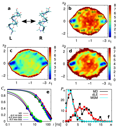
Figure 5: (a) Conformational transitions of the peptide Aib₉ from a left-handed (L) to a right-handed (R) helix. Energy landscape $\Delta{\cal G}$ along the first two principal components of the system, obtained from (b) $8\!\times\!2\ \mu$s-long unbiased MD simulations,Buchenberg15 (c) $\sim 7700$ 10 ns-long unbiased trajectories seeded by metadynamics,Biswas18 and (d) the dLE model. (e) Autocorrelation functions of the first two principal components, as obtained from long MD runs and various dLE models. (f) Probability of pathways, which use at least one main intermediate state and exactly $n$ middle states, obtained from long unbiased MD simulations, Buchenberg15 the MSM of Biswas et al.Biswas18 and the dLE model. A time resolution of 1 ns ( ) and 2 ps ( ) is used.

Judging from the prominent appearance of states (lllll), (rlllll), (rrlll),…, (rrrrr), (lrrrr), etc. in the free energy landscape, one might expect that a sequential pathway along these states provides the main way to get from L to R and back. These states are located at the external border of the energy landscape, while other states such as (rlrrr) are located inside the circle formed by the main states. This finding was questioned by an MSM pathway analysis of short implicit-solvent trajectories seeded by the MELD protocol,Perez15 which revealed that transitions involving lowly populated interior states nevertheless amounts to $\sim 40\%$ of the overall flux.Perez18 ; Nagel20 When we employ the $\sim 7700$ short unbiased trajectories seeded by metadynamics,Biswas18 Fig. 5c shows that the simulations indeed cover the entire energetically accessible energy landscape homogeneously. Since we deliberately started the short trajectories all over the place including high-energy regions such as barriers, however, this nonequilibrium energy landscape is not a good representation of the Boltzmann weighted free energy landscape.

To obtain the correct free energy landscape from this nonequilibrium data, we construct a dLE using a time step $\delta t\!=\!2\,$ps which ensures an adequate resolution of the dynamics. As described in Methods, we follow a recently proposed strategyLickert20 and rescale the friction and the noise fields by an overall factor ($S\sim 2$), such that resulting dLE model reproduces the initial decay of the position autocorrelation functions (see Methods). To be able to use all $\sim 4\cdot 10^{7}$ data points of the short trajectories, we applied a pre-averaging of the data to $10^{6}$ points (see SI). In total $10$ dLE trajectories of $20\,\mu$s length were simulated. Figure 5d shows the resulting free energy landscape, which is quite similar to the landscape obtained for the long unbiased MD simulations, except for a clearly better sampling of the lowly populated intermediate states. Due to the rescaling, MD and dLE also yield well matching autocorrelation functions of all five principal components (Fig. 5e and S4), showing that the first component decays on a $\sim 100\,$ns timescale, about an order of magnitude slower than the other components.

Adopting the state definition of Biswas et al.,Biswas18 we next calculate mean waiting times of various transitions between the ten most populated states and compared them to previous MSM results Biswas18 , see Fig. S5. We find good overall agreement of both approaches with an average deviation of 43 %. We obtain a similar conformance (average deviation of 50 %) with the waiting times from the long unbiased MD simulations, although this comparison only makes sense for the well-sampled main transitions of Aib₉. As an example, Table 2 compares the mean waiting time obtained for transitions between the two main states R and L. Being sampled 74 times by the long unbiased MD simulations, the MD results may serve as a reference. In comparison, the dLE results (full data) differ by 24 and 75 % for L$\rightarrow$R and R$\rightarrow$L, respectively, while the MSM results differ by 18 and 16 %.

	$\tau_{\text{L}\rightarrow\text{R}}$ [ns]	$\tau_{\text{R}\rightarrow\text{L}}$ [ns]
MD	$161\pm 23$	$80\pm 12$
MSM	$132\pm 0.2$	$67\pm 0.1$
dLE (full data)	$200\pm 8$	$140\pm 6$
dLE (short data)	$162\pm 6$	$113\pm 4$
dLE (less data)	$178\pm 6$	$132\pm 5$

Table 2: Average waiting times of the L$\leftrightarrow$R transitions of Aib₉, obtained for $8\!\times\!2\,\mu$s-long unbiased MD simulations, Buchenberg15 and for various models using short trajectories ($7700\!\times\!10\,$ns) of Biswas et al.Biswas18 as input data. Compared are a MSM,Biswas18 and various dLE models with full input data, and with shorter (4 ns) and fewer (2000) trajectories. Errors are calculated as standard deviations of the mean.

To characterize various types of L$\rightarrow$R transition pathways, Fig. 5f shows the probability $P_{n}$ of pathways, which use at least one main intermediate state and exactly $n$ middle states. In nice agreement, long unbiased MD and dLE simulations predict a unimodal distribution with a maximum for $n\approx 6$. As the MSM requires a minimum lag time of 1 ns, though, the resulting distribution is shifted towards shorter pathways with a peak at $n\approx 2.5$. Similar results are also obtained from MD and dLE, when a time resolution of 1 ns is used. Hence we find that, allowing for shorter time step than an MSM, the dLE may possibly provide a better time resolution of the dynamics.

To study the performance of the dLE for limited input data, we run two more sets of dLE simulations, where one set uses shorter ($7700\times 4\,$ns) and the other one fewer ($2000\times 10\,$ns) input trajectories. When we compare the resulting autocorrelation functions (Fig. 5e and S4) and the L$\leftrightarrow$R waiting times (Table 2) to results obtained for full input data, we again find that reduced input data in general leads to faster dynamics. This is particularly the case for shorter input data, which lead to a $\sim 20\,$% decrease of the L$\leftrightarrow$R waiting times. Similarly as found for the one-dimensional system in Sec. III.1, the five-dimensional dLE model for AiB₉ is shown to robustly predict the overall kinetics from nonequilibrium input data.

IV Conclusions

To extend the application of the data-driven Langevin equation (dLE) to the nonequilibrium regime, we have introduced various modifications of the original approach.Hegger09 ; Schaudinnus13 ; Schaudinnus15 ; Schaudinnus16 ; Lickert20 As a central result, we have shown that nonequilibrium conditions mainly affect the deterministic drift term $\boldsymbol{f}$ of the dLE (2). Compared to a system at thermal equilibrium which performs a Boltzmann sampling of the free energy landscape ($\boldsymbol{f}=-\partial_{\boldsymbol{x}}\Delta G(\boldsymbol{x})$), nonequilibrium processes sample the biased energy landscape

$$\Delta{\cal G}(\boldsymbol{x},t)=-k_{\rm B}T\ln{\cal P}(\boldsymbol{x})+V_{\rm ext}(\boldsymbol{x},t).$$ (21)

Here the first term accounts for the finite sampling in nonequilibrium simulations. For example, describing a relaxation process (Fig. 1a) with trajectories of length $t_{\rm max}$, ${\cal P}(\boldsymbol{x})$ reflects the conformational distribution sampled within $0\leq t\leq t_{\rm max}$. As a general result, we have found that too short input data bias the prediction towards too fast dynamics. The second term represents a time-dependent potential that accounts for the driving of the system. Considering, for example, an atomic force microscopy experiment that enforces the dissociation of a molecule (Fig. 1b), $V_{\rm ext}$ describes the gradual pulling of the system along the energy landscape. The biased energy landscape $\Delta{\cal G}(\boldsymbol{x},t)$ thus corresponds to the total deterministic potential experienced by the system at time $t$.

The dLE modeling of relaxation processes does not require additional assumptions compared to an equilibrium dLE. Indeed, for all considered examples of nonstationary preparation including hierarchical dynamics (Fig. 2), crystal nucleation (Fig. 4), and peptide conformational dynamics (Fig. 5), the resulting dLE model was shown to reproduce the reference data convincingly. On the other hand, it is in general an approximation that an external force leaves the friction $\Gamma$ and the noise $\mathcal{K}$ describing the system’s coupling to the bath unchanged. This assumption was shown to hold in the linear-response regime, which is expected to be valid for most biomolecular applications. For example, we found linear response behavior for the enforced dissociation of NaCl (Fig. 3) up to extremely high pulling velocities.Wolf18

Finally we have compared the dLE approach to the nonstationary GLE of Meyer et al.Meyer17 ; Meyer19 Studying crystal nucleation and enforced dissociation of NaCl, the GLE analysesMeyer20 ; Meyer21 resulted in slowly decaying memory kernels, which appears to question the applicability of a Markovian Langevin model such as the dLE. A theoretical analysis revealed that the LE (1) and the GLE (13) are based on different partitionings between system and bath, such that the former may well result in a Markovian system, although the latter exhibits non-Markovian behavior. The formulations thus provide a complementary description of nonequilibrium processes. The nonstationary GLE represents in principle an exact formulation, however, its memory kernel and the associated colored noise in general may be difficult to determine and interpret, in particular when we want to go beyond a one-dimensional phase space variable. While a Markovian LE model relies on a suitably chosen system coordinate, it represents a physically intuitive model, where the biased energy landscape $\Delta{\cal G}$ accounts for the main features of the considered process, and the friction $\Gamma$ and the noise $\mathcal{K}$ describe in a transparent way the effects of the bath. Moreover, the dLE algorithm allows us to use multidimensional coordinates $\boldsymbol{x}$ and fields $\boldsymbol{f}$, $\Gamma$ and $\mathcal{K}$ that depend on $\boldsymbol{x}$, which greatly adds to the versatility of the method.

Supporting Information

Details on the pre-averaging method, friction fields of the hierarchical model, noise checks of the nucleation model, as well as noise checks, autocorrelation functions, and mean waiting times of Aib₉.

The dLE algorithm as described in Ref. Schaudinnus16, including pre-averaging and rescaling is freely available at https://github.com/moldyn.

All data shown are available from the corresponding author upon reasonable request.

Acknowledgment

We thank Tanja Schilling and her group for helpful discussions and for sharing their trajectories of the crystal nucleation problem, as well as Matthias Post and Mithun Biswas for numerous instructive discussions. This work has been supported by the DFG via the Research Unit FOR5099 “Reducing complexity of nonequilibrium systems”, by the bwUniCluster computing initiative, the High Performance and Cloud Computing Group at the Zentrum für Datenverarbeitung of the University of Tübingen, the state of Baden-Württemberg through bwHPC and the DFG through grant No. INST 37/935-1 FUGG.

References

- (1) H. J. C. Berendsen, Simulating the Physical World, Cambridge University Press, Cambridge, 2007.
- (2) M. A. Rohrdanz, W. Zheng, and C. Clementi, Discovering mountain passes via torchlight: Methods for the definition of reaction coordinates and pathways in complex macromolecular reactions, Annu. Rev. Phys. Chem. 64, 295 (2013).
- (3) B. Peters, Reaction coordinates and mechanistic hypothesis tests, Annu. Rev. Phys. Chem. 67, 669 (2016).
- (4) F. Sittel and G. Stock, Perspective: Identification of collective coordinates and metastable states of protein dynamics, J. Chem. Phys. 149, 150901 (2018).
- (5) H. Grabert, P. Hänggi, and P. Talkner, Microdynamics and nonlinear stochastic processes of gross variables, J. Stat. Phys. 22, 537 – 552 (1980).
- (6) R. Kubo, M. Toda, and N. Hashitsume, Statistical Physics II. Nonequilibrium Statistical Mechanics, Springer, Berlin, 1985.
- (7) R. Zwanzig, Nonequilibrium Statistical Mechanics, Oxford University, Oxford, 2001.
- (8) R. Hernandez, The projection of a mechanical system onto the irreversible generalized Langevin equation, J. Chem. Phys. 111, 7701 (1999).
- (9) M. McPhie, P. Daivis, I. Snook, J. Ennis, and D. Evans, Generalized Langevin equation for nonequilibrium systems, Physica A 299, 412 (2001).
- (10) C. Micheletti, G. Bussi, and A. Laio, Optimal Langevin modeling of out-of-equilibrium molecular dynamics simulations, J. Chem. Phys. 129, 074105 (2008).
- (11) S. Kawai and T. Komatsuzaki, Derivation of the generalized Langevin equation in nonstationary environments, J. Chem. Phys. 134, 114523 (2011).
- (12) H. Meyer, T. Voigtmann, and T. Schilling, On the non-stationary generalized Langevin equation, J. Chem. Phys. 147, 214110 (2017).
- (13) H. Meyer, T. Voigtmann, and T. Schilling, On the dynamics of reaction coordinates in classical, time-dependent, many-body processes, J. Chem. Phys. 150, 174118 (2019).
- (14) B. Cui and A. Zaccone, Generalized Langevin equation and fluctuation-dissipation theorem for particle-bath systems in external oscillating fields, Phys. Rev. E 97, 060102 (2018).
- (15) R. Zwanzig, Nonlinear generalized Langevin equations, J. Stat. Phys. 9, 215 (1973).
- (16) J. E. Straub, M. Borkovec, and B. J. Berne, Calculation of dynamic friction on intramolecular degrees of freedom, J. Phys. Chem. 91, 4995 (1987).
- (17) G. Hummer, Position-dependent diffusion coefficients and free energies from Bayesian analysis of equilibrium and replica molecular dynamics simulations, New J. Phys. 7, 34 (2005).
- (18) R. B. Best and G. Hummer, Diffusive model of protein folding dynamics with Kramers turnover in rate, Phys. Rev. Lett. 96, 228104 (2006).
- (19) O. F. Lange and H. Grubmüller, Collective Langevin dynamics of conformational motions in proteins, J. Chem. Phys. 124, 214903 (2006).
- (20) M. Hinczewski, Y. von Hansen, J. Dzubiella, and R. R. Netz, How the diffusivity profile reduces the arbitrariness of protein folding free energies, J. Chem. Phys. 132, 245103 (2010).
- (21) A. Perez-Villa and F. Pietrucci, Free energy, friction, and mass profiles from short molecular dynamics trajectories, arXiv 1810.00713 (2018).
- (22) S. Wolf and G. Stock, Targeted molecular dynamics calculations of free energy profiles using a nonequilibrium friction correction, J. Chem. Theory Comput. 14, 6175 (2018).
- (23) F. Paul, H. Wu, M. Vossel, B. L. de Groot, and F. Noé, Identification of kinetic order parameters for non-equilibrium dynamics, J. Chem. Phys. 150, 164120 (2019).
- (24) R. Hegger and G. Stock, Multidimensional Langevin modeling of biomolecular dynamics, J. Chem. Phys. 130, 034106 (2009).
- (25) N. Schaudinnus, A. J. Rzepiela, R. Hegger, and G. Stock, Data driven Langevin modeling of biomolecular dynamics, J. Chem. Phys. 138, 204106 (2013).
- (26) N. Schaudinnus, B. Bastian, R. Hegger, and G. Stock, Multidimensional Langevin modeling of nonoverdamped dynamics, Phys. Rev. Lett. 115, 050602 (2015).
- (27) N. Schaudinnus, B. Lickert, M. Biswas, and G. Stock, Global Langevin model of multidimensional biomolecular dynamics, J. Chem. Phys. 145, 184114 (2016).
- (28) B. Lickert and G. Stock, Modeling non-Markovian data using Markov state and Langevin models, J. Chem. Phys. 153, 244112 (2020).
- (29) H. Meyer, S. Wolf, G. Stock, and T. Schilling, A numerical procedure to evaluate memory effects in non-equilibrium coarse-grained models, Adv. Theory Simul. 111, 2000197 (2020).
- (30) H. Meyer, F. Glatzel, W. Wöhler, and T. Schilling, Evaluation of memory effects at phase transitions and during relaxation processes, Phys. Rev. E 103, 022102 (2021).
- (31) A. J. Rzepiela, N. Schaudinnus, S. Buchenberg, R. Hegger, and G. Stock, Communication: Microsecond peptide dynamics from nanosecond trajectories: A Langevin approach, J. Chem. Phys. 141, 241102 (2014).
- (32) S. Buchenberg, N. Schaudinnus, and G. Stock, Hierarchical biomolecular dynamics: Picosecond hydrogen bonding regulates microsecond conformational transitions, J. Chem. Theory Comput. 11, 1330 (2015).
- (33) M. Biswas, B. Lickert, and G. Stock, Metadynamics enhanced Markov modeling: Protein dynamics from short trajectories, J. Phys. Chem. B 122, 5508 (2018).
- (34) P. Grassberger, An optimized box-assisted algorithm for fractal dimensions, Phys. Lett. A 148, 63 (1990).
- (35) M. Post, S. Wolf, and G. Stock, Principal component analysis of nonequilibrium molecular dynamics simulations, J. Chem. Phys. 150, 204110 (2019).
- (36) J. O. Daldrop, B. G. Kowalik, and R. R. Netz, External potential modifies friction of molecular solutes in water, Phys. Rev. X 7, 041065 (2017).
- (37) D. Chandler, Introduction to Modern Statistical Mechanics, Oxford University, Oxford, 1987.
- (38) H. Grubmüller, B. Heymann, and P. Tavan, Ligand binding: Molecular mechanics calculation of the streptavidin-biotin rupture force, Science 271, 997 (1996).
- (39) B. Isralewitz, M. Gao, and K. Schulten, Steered molecular dynamics and mechanical functions of proteins, Curr. Opin. Struct. Biol. 11, 224 (2001).
- (40) S. Park and K. Schulten, Calculating potentials of mean force from steered molecular dynamics simulations, J. Chem. Phys. 120, 5946 (2004).
- (41) H. Frauenfelder, S. Sligar, and P. Wolynes, The energy landscapes and motions of proteins, Science 254, 1598 (1991).
- (42) K. Henzler-Wildman and D. Kern, Dynamic personalities of proteins, Nature (London) 450, 964 (2007).
- (43) S. Buchenberg, F. Sittel, and G. Stock, Time-resolved observation of protein allosteric communication, Proc. Natl. Acad. Sci. USA 114, E6804 (2017).
- (44) O. Bozovic, C. Zanobini, A. Gulzar, B. Jankovic, D. Buhrke, M. Post, S. Wolf, G. Stock, and P. Hamm, Real-time observation of ligand-induced allosteric transitions in a PDZ domain, Proc. Natl. Acad. Sci. USA 117, 26031 (2020).
- (45) R. Gernert, C. Emary, and S. Klapp, Waiting time distribution for continous stochastic systems, Phys. Rev. E 90, 062115 (2014).
- (46) S. Wolf, B. Lickert, S. Bray, and G. Stock, Multisecond ligand dissociation dynamics from atomistic simulations, Nat. Commun. 11, 2918 (2020).
- (47) M. J. Abraham, T. Murtola, R. Schulz, S. Pall, J. C. Smith, B. Hess, and E. Lindahl, Gromacs: High performance molecular simulations through multi-level parallelism from laptops to supercomputers, SoftwareX 1, 19 (2015).
- (48) V. Hornak, R. Abel, A. Okur, B. Strockbine, A. Roitberg, and C. Simmerling, Comparison of multiple Amber force fields and development of improved protein backbone parameters, Proteins 65, 712 (2006).
- (49) R. B. Best and G. Hummer, Optimized molecular dynamics force fields applied to the helix-coil transition of polypeptides, J. Phys. Chem. B 113, 9004 (2009).
- (50) W. L. Jorgensen, J. Chandrasekhar, J. D. Madura, R. W. Impey, and M. Klein, Comparison of simple potential functions for simulating liquid water, J. Chem. Phys. 79, 926 (1983).
- (51) R. G. Mullen, J.-E. Shea, and B. Peters, Transmission Coefficients, Committors, and Solvent Coordinates in Ion-Pair Dissociation, J. Chem. Theory Comput. 10, 659 (2014).
- (52) A. Kuhnhold, H. Meyer, G. Amati, P. Pelagejcev, and T. Schilling, Derivation of an exact, nonequilibrium framework for nucleation: Nucleation is a priori neither diffusive nor markovian, Phys. Rev. E 100, 052140 (2019).
- (53) P. R. ten Wolde, M. J. Ruiz-Montero, and D. Frenkel, Numerical evidence for bcc ordering at the surface of a critical fcc nucleus, Phys. Rev. Lett. 75, 2714 (1995).
- (54) G. R. Bowman, K. A. Beauchamp, G. Boxer, and V. S. Pande, Progress and challenges in the automated construction of Markov state models for full protein systems, J. Chem. Phys. 131, 124101 (2009).
- (55) J.-H. Prinz, H. Wu, M. Sarich, B. Keller, M. Senne, M. Held, J. D. Chodera, C. Schütte, and F. Noé, Markov models of molecular kinetics: generation and validation, J. Chem. Phys. 134, 174105 (2011).
- (56) G. R. Bowman, V. S. Pande, and F. Noé, An Introduction to Markov State Models, Springer, Heidelberg, 2013.
- (57) A. Perez, F. Sittel, G. Stock, and K. Dill, Meld-path efficiently computes conformational transitions, including multiple and diverse paths, J. Chem. Theory Comput. 14, 2109 (2018).
- (58) A. Laio and M. Parrinello, Escaping free-energy minima, Proc. Natl. Acad. Sci. USA 99, 12562 (2002).
- (59) G. Bussi, A. Laio, and P. Tiwary, Metadynamics: A Unified Framework for Accelerating Rare Events and Sampling Thermodynamics and Kinetics, pages 565–595, Springer International Publishing, Cham, 2020.
- (60) W. F. van Gunsteren, S. R. Billeter, A. A. Eising, P. H. Hünenberger, P. Krüger, A. E. Mark, W. R. P. Scott, and I. G. Tironi, Biomolecular Simulation: The GROMOS96 Manual and User Guide, Vdf Hochschulverlag AG an der ETH Zürich, Zürich, 1996.
- (61) I. G. Tironi and W. F. van Gunsteren, A molecular dynamics simulation study of chloroform, Mol. Phys. 83, 381 (1994).
- (62) A. Altis, M. Otten, P. H. Nguyen, R. Hegger, and G. Stock, Construction of the free energy landscape of biomolecules via dihedral angle principal component analysis, J. Chem. Phys. 128, 245102 (2008).
- (63) F. Sittel, T. Filk, and G. Stock, Principal component analysis on a torus: Theory and application to protein dynamics, J. Chem. Phys. 147, 244101 (2017).
- (64) F. Sittel and G. Stock, Robust density-based clustering to identify metastable conformational states of proteins, J. Chem. Theory Comput. 12, 2426 (2016).
- (65) A. Perez, J. L. MacCallum, and K. Dill, Accelerating molecular simulations of proteins using Bayesian inference on weak information., Proc. Natl. Acad. Sci. USA 112, 11846 (2015).
- (66) D. Nagel, A. Weber, and G. Stock, MSMPathfinder: Identification of pathways in Markov state models, J. Chem. Theory Comput. 16, 7874 (2020).