Adaptive estimation in symmetric location model under log-concavity constraint

Abstract

We revisit the problem of estimating the center of symmetry $\theta$ of an unknown symmetric density $f$. Although Stone (1975), Van Eeden (1970), and Sacks (1975) constructed adaptive estimators of $\theta$ in this model, their estimators depend on external tuning parameters. In an effort to reduce the burden of tuning parameters, we impose an additional restriction of log-concavity on $f$. We construct truncated one-step estimators which are adaptive under the log-concavity assumption. Our simulations suggest that the untruncated version of the one step estimator, which is tuning parameter free, is also asymptotically efficient. We also study the maximum likelihood estimator (MLE) of $\theta$ in the shape-restricted model.

1 Introduction

In this paper, we revisit the symmetric location model with an additional shape-restriction of log-concavity. We let $\mathcal{P}$ denote the class of all densities on the real line $\mathbb{R}$. For any $\theta\in\mathbb{R}$, denote by $\mathcal{S}_{\theta}$ the class of all densities symmetric about $\theta$. Then the symmetric location model $\mathcal{P}_{s}$ is given by

$$\mathcal{P}_{s}=\bigg{\{}f\in\mathcal{P}\ \bigg{|}\ f(x;\theta)=g(x-\theta),\ \theta\in\mathbb{R},\ g\in\mathcal{S}_{0},\ \mathcal{I}_{f}<\infty\bigg{\}},$$ (1)

where $\mathcal{I}_{f}$ is the Fisher information for location. It is well-established that (Huber, 1964, Theorem 3) $\mathcal{I}_{f}$ is finite if and only if $f$ is an absolutely continuous density satisfying

$$\int_{-\infty}^{\infty}\bigg{(}\dfrac{f^{\prime}(x)}{f(x)}\bigg{)}^{2}f(x)dx<\infty,$$

where $f^{\prime}$ is an $L_{1}$-derivative of $f$. Also, in this case, $\mathcal{I}_{f}$ takes the form

$$\mathcal{I}_{f}=\displaystyle\int_{-\infty}^{\infty}\bigg{(}\dfrac{f^{\prime}(x)}{f(x)}\bigg{)}^{2}f(x)dx.$$

Estimation of $\theta$ in $\mathcal{P}_{s}$ is an old semi-parametric problem, dating back to Stein (1956). From then on, the problem of estimating $\theta_{0}$ in $\mathcal{P}_{s}$ has been considered by many early authors including, but not limited to, Stone (1975), Beran (1974), Sacks (1975), and Van Eeden (1970). There are two main reasons behind the assumption of symmetry in this model. First, as Stone has pointed out, if $f$ is totally unrestricted, $\theta$ is not identifiable. Second, the definition of location becomes unclear in the absence of symmetry (Takeuchi, 1975). The appeal of the above model lies in the fact that adaptive estimation of $\theta$ is possible in this model (Stone, 1975). In other words, there exist consistent estimators of $\theta$ in $\mathcal{P}_{s}$, whose asymptotic variance attains the parametric lower bound, which is $\mathcal{I}_{f}^{-1}$ in this case. See Sections $3.2$, $3.3$, and $6.3$ of Bickel et al. (1998) for more discussion on adaptive estimation in $\mathcal{P}_{s}$.

There are general classes of nonparametric estimators, which, following some clever reconstruction, lead to adaptive estimators of $\theta$ in $\mathcal{P}_{s}$. Examples include the one step estimator used by Stone, and the Hodges-Lehmann rank estimator used by Van Eeden. Beran uses a linearized rank estimator introduced by Kraft and Van Eeden (1970), where Sacks uses a linear functional of order statistics. All these estimators involve various tuning parameters. The success of these type of nonparametric estimators generally depend crucially on the choice of the tuning parameters. (cf. Sacks (1975); see also Park (1990) for a thorough empirical study of similar estimators in a closely related nonparametric problem, i.e. the two-sample location problem.) However, no data-dependent method has been prescribed to choose these tuning parameters. Therefore, despite attractive theoretical properties, the implementation of the asymptotically efficient estimators of $\theta_{0}$ is not straightforward.

Although the tuning parameters stemming from different nonparametric approaches appear to be different, they generally fall in one of the following categories: (a) scaling parameter for approximating derivatives by quotient (e.g. Beran, Sacks and Van Eeden), (b) bandwidth selection parameter if kernels are used (e.g. Stone), (c) the number of basis functions (e.g. Beran), (d) parameters arising due to truncation (e.g. the estimators of Stone and Sacks) or data-partitioning (e.g., Van Eeden). We will elaborate a little bit on the first three type of tuning parameters. They arise solely because the adaptive estimators of $\theta_{0}$ require estimating $g$, $g^{\prime}$ (e.g. Stone, Van Eeden, and Beran), and in some cases, higher derivatives (e.g. $g^{\prime\prime}$, Sacks). In fact, such tuning parameters are unavoidable in nonparametric estimation of the above quantities. Moreover, Hogg (1974) points out that in practice, nonparametric estimation of such functions may be too slow. This is precisely where semi-parametric models can help because the additional structure can be exploited to construct computationally efficient estimators of $g$ and $g^{\prime}$ without using tuning parameters.

If we impose an additional shape restriction of log-concavity on $g$, for instance, the task of estimating $g^{\prime}$ becomes much simpler. The reason is, the class of log-concave densities is structurally rich enough to admit a maximum likelihood estimator (MLE) (Pal et al., 2007; Dümbgen and Rufibach, 2009). Similar results hold for its subclasses, e.g. the class of all symmetric (about the origin) log-concave densities as well (Doss and Wellner, 2019b). The log-concave MLE type density estimators allow for computationally efficient estimation of the scores without any tuning parameters. These score estimates can readily be used to construct a one step estimator.

We show that under the log-concavity assumption, truncated versions of the above-mentioned one step estimator are adaptive provided the truncation parameter $\eta_{n}\to 0$ slowly enough. This truncation parameter is our only tuning parameter, which also is introduced purely due to technical reasons in the proof. Moreover, we empirically show that the efficiency of our estimators monotonously increases as $\eta_{n}\to 0$. In fact, the untruncated one step estimator attains the highest efficiency, and also performs reliably under varied settings. Thus, for practical implementation, the proposed estimator of this paper is the untruncated one-step estimator, which is fully tuning parameter free. We also touch upon another important tuning parameter free estimator of $\theta_{0}$, namely the MLE. In particular, we establish its existence under the shape-constrained model. Our methods can be implemented using the R package log.location which can be accessed at https://github.com/nilanjanalaha/log.location.

The imposition of log-concavity on $\mathcal{P}_{s}$ may seem forced, but is not at all unnatural. The class of log-concave densities, $\mathcal{LC}$, is an important subclass of the class of unimodal densities. Many common symmetric unimodal densities, e.g. Gaussian, logistic, and Laplace, are log-concave. Unimodality is a reasonable assumption in context of location estimation of symmetric densities. As Takeuchi (1975) points out, in practice, multimodal densities generally result from unimodal mixtures. Separate procedures are available for the latter class. The difficulty with the unimodality shape restriction, however, stems from the fact that the corresponding density-class is still large, especially it is not structurally rich enough to admit an MLE (Birgé, 1997). Therefore unlike the log-concavity assumption, the unimodality assumption does not provide computational advantages. Hence, we impose the assumption of log-concavity on $\mathcal{P}_{s}$ instead of just unimodality.

Finally, this paper is an attempt towards bridging the gap between the symmetric location model and log-concavity. Although shape-constrained estimation has a rich history, so far there has been little to no use of shape-constraints in one-sample symmetric location problem. In fact, to the best of our knowledge, Van Eeden (1970) is the only one to incorporate shape-constraints in treating the problem considered here. Actually Van Eeden requires $f$ to be log-concave although her paper does not mention log-concavity. She requires the function $f^{\prime}(F^{-1}(u))/f(F^{-1}(u))$ to be non-increasing in $u\in(0,1)$, which is equivalent to $f$ being log-concave (Bobkov, 1996, Proposition A.1). As made clear by our earlier discussion, Van Eeden does not use shape-restricted tools tailored for log-concave densities because they were not available at that time. We also want to mention Bhattacharyya and Bickel (2013), who consider both location and scale estimation in an elliptical symmetry model, which albeit bearing some resemblance, is different from the model considered in this paper. Also, Bhattacharyya and Bickel (2013)’s estimation procedure is completely different from ours.

1.1 Notation and terminology

For a concave function $\psi:\mathbb{R}\mapsto\mathbb{R}$, the domain $\mathrm{dom}(\psi)$ will be defined as in (Rockafellar, 1970, p. 40), that is, $\mathrm{dom}(\psi)=\{x\in\mathbb{R}\ :\ \psi(x)>-\infty\}$. For any concave function $\psi$, we say $x\in\mathbb{R}$ is a knot of $\psi$, if either $\psi^{\prime}(x+)\neq\psi^{\prime}(x-)$, or $x$ is at the boundary of $\mathrm{dom}(\psi)$. We denote by $\mathcal{K}(\psi)$ the set of the knots of $\psi$. Unless otherwise mentioned, for a real valued function $h$, provided they exist, $h^{\prime}$ and $h^{\prime}(\mathord{\cdot}-)$ will refer to the right and left derivatives of $h$, respectively. We denote the support of any density $f$ by $\text{supp}(f)=\{x\in\mathbb{R}\ :\ f(x)>0\}$.

For a distribution function $F$, we let $J(F)$ denote the set $\{x\ :\ 0<F(x)<1\}$. For a sequence of distribution functions $\{F_{n}\}_{n\geq 1}$, we say $F_{n}$ converges weakly to $F$, and write $F_{n}\to_{d}F$, if for all bounded continuous functions $h:\mathbb{R}\mapsto\mathbb{R}$, we have $\lim\limits_{n\to\infty}\int hdF_{n}=\int hdF$. For any real valued function $h:\mathbb{R}\mapsto\mathbb{R}$, we let $||h||_{k}$ denote its $L_{k}$ norm, i.e.

$$||h||_{k}=\bigg{(}\displaystyle\int_{-\infty}^{\infty}|h(x)|^{k}dx\bigg{)}^{1/k},\quad k\geq 1.$$

For densities $f_{1}$ and $f_{2}$, the Hellinger distance $H(f_{1},f_{2})$ is defined by

$$H^{2}(f_{1},f_{2})=\frac{1}{2}\displaystyle\int_{-\infty}^{\infty}(\sqrt{f}_{1}(x)-\sqrt{f}_{2}(x))^{2}dx.$$

We denote the order statistics of a random sample $(Y_{1},\ldots,Y_{n})$ by $(Y_{(1)},\ldots,Y_{(n)})$.

As usual, we denote the set of natural numbers by $\mathbb{N}$. We denote by $C$ an arbitrary constant which may vary from line to line. The expression $x\lesssim y$ will imply that there exists $C>0$ so that $x\leq Cy$.

1.2 Problem set up

To formalize the set up, first, let us define

$$\mathcal{C}:=\bigg{\{}\phi:\mathbb{R}\mapsto[-\infty,\infty)\ \bigg{|}\ \phi\text{ is concave, closed, and proper}\bigg{\}}.$$ (2)

We let $\mathcal{SC}_{\theta}=\mathcal{S}_{\theta}\cap\mathcal{C}$ denote the class of all closed and proper concave functions symmetric about $\theta\in\mathbb{R}$. Here a proper and closed concave function is as defined in Rockafellar (1970), page 24 and 50. Letting $\mathcal{LC}$ denote the class of log-concave densities

$$\mathcal{LC}:=\bigg{\{}f\in\mathcal{P}\ \bigg{|}\ \phi=\log f\in\mathcal{C}\bigg{\}},$$

we set $\mathcal{SLC}_{\theta}=\mathcal{LC}\cap\mathcal{S}_{\theta}$. Suppose we observe $n$ independent and identically distributed (i.i.d.) random variables $X\equiv X_{1},\ldots,X_{n}$ with density $f_{0}\equiv g_{0}(\cdot-\theta_{0})\in\mathcal{P}_{0}$, where

$$\mathcal{P}_{0}=\bigg{\{}f\in\mathcal{P}\ \bigg{|}\ f(x;\theta)=g(x-\theta),\ \theta\in\mathbb{R},\ g\in\mathcal{SLC}_{0},\ \mathcal{I}_{g}<\infty\bigg{\}}$$ (3)

is the symmetric log-concave location model. Our aim is to estimate the location parameter $\theta_{0}$.

Let us denote $\phi_{0}=\log f_{0}$, and $\psi_{0}=\log g_{0}$. We let $F_{0}$ and $G_{0}$ be the respective distribution functions of $f_{0}$ and $g_{0}$, and denote by $P_{0}$ the measure corresponding to $F_{0}$. We denote the empirical distribution function of the $X_{i}$’s by $\mathbb{F}_{n}$, and write $\mathbb{P}_{n}$ for the corresponding empirical measure.

We use the following convention throughout the paper while setting notations for the one step estimators and the MLE. We use a hat on the quantities related to the MLE, e.g. the MLE of $\theta_{0}$ and $g_{0}$ will be denoted by $\widehat{\theta}_{n}$ and $\widehat{g}_{n}$, respectively. The similar quantities in the one-step estimator context will use a tilde, e.g. $\tilde{\theta}_{n}$, $\tilde{g}_{n}$ etc. Some quantities like $\widehat{h}_{n}$, the MLE in $\mathcal{LC}$, or $\widehat{f}_{\theta}$, the MLE in $\mathcal{SLC}_{\theta}$, will be introduced in context of the one step estimators, but their notations use the hat instead of the tilde because they are MLEs.

The article is organized as follows. In Section 2, we introduce the one step estimator, and discuss its asymptotic properties. In Section 3, we explore the MLE of $\theta_{0}$ in $\mathcal{P}_{0}$. We provide an empirical study in Section 4. The proofs are deferred to the appendix.

2 One step estimator

Let $\bar{\theta}_{n}$ be a preliminary estimator of $\theta_{0}$. Had $g_{0}$ been known, a valid estimator of $\theta_{0}$ would be readily given by the one step estimator (see p. 71-72 and 392-399 of Van der Vaart, 1998)

$$\bar{\theta}_{n}-\displaystyle\int_{-\infty}^{\infty}\dfrac{{\psi}^{\prime}_{0}(x-\bar{\theta}_{n})}{\mathcal{I}_{f_{0}}}d\mathbb{F}_{n}(x).$$ (4)

In fact, the above estimator is $\sqrt{n}$ consistent with asymptotic variance $\mathcal{I}_{f_{0}}^{-1}$ when $g_{0}$ is known (cf. Theorem 5.45 of Van der Vaart, 1998). Suppose $\tilde{g}_{n}\in\mathcal{S}_{0}$ is an estimator of $g_{0}$. Further suppose $\tilde{\psi}_{n}=\log\tilde{g}_{n}$ is left and right differentiable on the support of $\tilde{g}_{n}$. The latter always holds if $\tilde{g}_{n}\in\mathcal{LC}$ (Theorem 0.6.3, pp.15, Hiriart-Urruty and Lemaréchal, 2004). Suppose $\tilde{\psi}_{n}^{\prime}$ is the right derivative of $\tilde{\psi}_{n}$. Defining $\tilde{\psi}_{n}^{\prime}$ to be zero outside $\text{supp}(\tilde{g}_{n})$, we can define an estimator of $\theta_{0}$ along the lines of (4) as follows:

$$\widehat{\theta}_{n,0}=\bar{\theta}_{n}-\displaystyle\int_{-\infty}^{\infty}\dfrac{\tilde{\psi}^{\prime}_{n}(x-\bar{\theta}_{n})}{\widehat{\mathcal{I}}_{n}}d\mathbb{F}_{n}(x),$$ (5)

where

$$\widehat{\mathcal{I}}_{n}=\displaystyle\int_{-\infty}^{\infty}\tilde{\psi}^{\prime}_{n}(x-\bar{\theta}_{n})^{2}d\mathbb{F}_{n}(x)$$ (6)

is an estimator of the Fisher information $\mathcal{I}_{f_{0}}$. We will refer to $\widehat{\theta}_{n,0}$ as the untruncated one step estimator.

The asymptotic behavior of $\tilde{\psi}_{n}^{\prime}$ can be hard to control in the tails, which creates technical difficulties in the asymptotic analysis of $\widehat{\theta}_{n,0}$. As we already mentioned in the introduction, a common approach to tackle this problem is trimming the extreme observations, which leads to a truncated one step estimator similar to Stone.

We let $\eta_{n}$ denote the truncation parameter, which is usually a small positive fraction. Denote by $\tilde{G}_{n}$ the distribution function corresponding to $\tilde{g}_{n}$. Letting $\xi_{n}$ be the $(1-\eta_{n})$-th quantile of $\tilde{G}_{n}$, we define the truncated one step estimator as follows:

$$\tilde{\theta}_{n}=\bar{\theta}_{n}-\displaystyle\int_{\bar{\theta}_{n}-\xi_{n}}^{\bar{\theta}_{n}+\xi_{n}}\dfrac{\tilde{\psi}_{n}^{\prime}(x-\bar{\theta}_{n})}{\widehat{\mathcal{I}}_{n}(\eta_{n})}d\mathbb{F}_{n}(x).$$ (7)

Here $\widehat{\mathcal{I}}_{n}(\eta_{n})$ is a truncated version of $\widehat{\mathcal{I}}_{n}$, given by

$$\widehat{\mathcal{I}}_{n}(\eta_{n})=\displaystyle\int_{\bar{\theta}_{n}-\xi_{n}}^{\bar{\theta}_{n}+\xi_{n}}\tilde{\psi}^{\prime}_{n}(x-\bar{\theta}_{n})^{2}d\mathbb{F}_{n}(x).$$ (8)

Note that the symmetry of $\tilde{g}_{n}$ about $0$ implies that $-\xi_{n}=\tilde{G}_{n}^{-1}(\eta_{n})$. Ideally, we should denote the one step estimator in (7) by $\tilde{\theta}_{n}(\eta_{n})$ but here we suppress the dependence on $\eta_{n}$ to avoid cumbersome notation.

$\mathcal{I}_{f_{0}}$ could also be estimated by a smoother version of $\widehat{\mathcal{I}}_{n}(\eta_{n})$, namely,

$$\widehat{\mathcal{I}}_{n}^{*}(\eta_{n})=\displaystyle\int_{\bar{\theta}_{n}-\xi_{n}}^{\bar{\theta}_{n}+\xi_{n}}\tilde{\psi}^{\prime}_{n}(x-\bar{\theta}_{n})^{2}\tilde{g}_{n}(x-\bar{\theta}_{n})dx.$$

However, our simulations indicate that the estimator $\widehat{\mathcal{I}}_{n}(\eta)$ yields a more efficient one-step estimator. Therefore, $\widehat{\mathcal{I}}_{n}(\eta)$ is our preferred estimator for the Fisher information.

2.1 Main result

The first main result of this paper implies that if $\eta_{n}\to 0$ at a sufficiently slow rate, then the truncated one step estimator defined in (7) is adaptive for certain choices of $\tilde{g}_{n}$. However, we require a technical assumption on $\psi_{0}$ to prove this theorem.

Assumption A.

There exists $\kappa>0$ so that

$$|\psi_{0}^{\prime}(x)-\psi^{\prime}_{0}(y)|\leq\kappa|x-y|\quad\text{ for all }x,y\in\mathrm{int}(\mathrm{dom}(\psi_{0})),$$

where $\psi_{0}^{\prime}(x)$ (or $\psi_{0}^{\prime}(y)$) is either the left or right derivative of $\psi_{0}$ at $x$ (or $y$).

Since $\psi_{0}$ is concave, it is left and right differentiable at every $x\in\mathrm{int}(\mathrm{dom}(\psi_{0}))$ (pp. 15 Hiriart-Urruty and Lemaréchal, 2004). If $\psi_{0}$ is twice differentiable on $\mathrm{int}(\mathrm{dom}(\psi_{0}))$, Assumption A interprets as $|\psi_{0}^{\prime\prime}|\leq\kappa$. Assumption A is essentially a smoothness condition, which is not uncommon in the context of log-concave density estimation. A similar assumption appears in Dümbgen and Rufibach (2009) (see Theorem 4.1 therein), who consider $\psi_{0}$ to be in a Hölder class with exponent $\beta\in[1,2]$, which coincides with Assumption A if $\beta=2$. The Hölder-smoothness assumption is also used in Doss and Wellner (2019a) (see Theorem 2.1 therein), who generalize Dümbgen and Rufibach (2009)’s Theorem 4.1 to the case of unimodal log-concave densities. Such smoothness assumptions can also be found in the literature related to monotonocity constraints Kuchibhotla et al. (2017); Mukherjee and Sen (2018). Simple algebra shows that common symmetric log-concave densities like Gaussian, Laplace, and Logistic satisfy Assumption A. Later in Section 4, we consider an example where Assumption A is violated. Whether Assumption A is necessary is unknown to us, although Section 4 hints that the truncated one step estimators may still be adaptive even under the violation of Assumption A.

Now we state the requirements for $\tilde{g}_{n}$. Later in this section, we demonstrate how to build estimators which satisfy such conditions.

Condition 1.

Let $y_{n}=o_{p}(1)$ be a random sequence. The density estimator $\tilde{g}_{n}$ satisfies the following:

• $\|\tilde{g}_{n}-g_{0}\|_{1}\to_{p}0$ and $\sup_{x\in\mathbb{R}}|\tilde{g}_{n}(x+y_{n})-g_{0}(x)|\to_{p}0$.

• For any $K\subset\mathrm{int}(\mathrm{dom}(\psi_{0}))$, we have $\sup_{x\in K}|\tilde{\psi}_{n}(x+y_{n})-\psi_{0}(x)|\to_{p}0.$

• Suppose $x\in\mathrm{int}(\mathrm{dom}(\psi_{0}))$ is a continuity point of $\psi_{0}^{\prime}.$ Then

  $$\tilde{\psi}_{n}^{\prime}(x+y_{n})\to_{p}\psi_{0}^{\prime}(x).$$

Condition 1 (A) implies $H(\tilde{g}_{n},g_{0})\to_{p}0$ because $H(\tilde{g}_{n},g_{0})\lesssim\sqrt{\|\tilde{g}_{n}-g_{0}\|_{1}}$. However, we require stronger control over the rate of decay of the Hellinger error $H(\tilde{g}_{n},g_{0})$.

Condition 2.

There exists $p\in(0,1/2]$ so that $H(\tilde{g}_{n},g_{0})=O_{p}(n^{-p})$.

The upper bound of $1/2$ on $p$ is natural because even in the parametric case, the Hellinger error rate is generally not faster than $O_{p}(n^{-1/2})$. Now we are ready to state our main theorem. The proof of Theorem 1 can be found in Appendix A.

Theorem 1.

Suppose $f_{0}\in\mathcal{P}_{0}$ satisfies Assumption A and $\bar{\theta}_{n}$ is a $\sqrt{n}$-consistent estimator of $\theta_{0}$. Let $\tilde{g}_{n}\in\mathcal{SLC}_{0}$ be an estimator of $g_{0}$ which satisfies Conditions 1 and 2. Suppose $\eta_{n}=Cn^{-2p^{\prime}/5}$, where $C>0$ is any constant, and $p^{\prime}\in(0,p]$, where $p$ is as in Condition 2. Then the estimator $\tilde{\theta}_{n}$ defined in (7) satisfies

$$\sqrt{n}(\tilde{\theta}_{n}-\theta_{0})\to_{d}N(0,\mathcal{I}_{f_{0}}^{-1}).$$

A couple of remarks are in order. First, Theorem 1 requires $\tilde{g}_{n}\in\mathcal{SLC}_{0}$. This automatically rules out most nonparametric density estimators including the symmetrized kernel density estimator of Stone. Second, Theorem 1 requires $\bar{\theta}_{n}$ to be $\sqrt{n}$-consistent. Stone and Beran impose similar conditions on their preliminary estimators. The $Z$-estimator of the shift in the logistic location shift model is $\sqrt{n}$-consistent under minimal regularity conditions (cf. Example 5.40 and Theorem $5.23$, Van der Vaart, 1998). When $f_{0}\in\mathcal{P}_{0}$, the sample mean and the sample median also satisfy this requirement.

Now we give example of two $\tilde{g}_{n}$’s, which satisfy the conditions of Theorem 1.

Partial MLE estimator $\widehat{g}_{\bar{\theta}_{n}}$: For any $\theta\in\mathbb{R}$, the density class $\mathcal{SLC}_{\theta}$ admits an MLE (Theorem 2.1(C), Doss and Wellner, 2019b). When $\theta=\bar{\theta}_{n}$, the MLE in the class $\mathcal{SLC}_{\bar{\theta}_{n}}$ is a legitimate estimator of $f_{0}$. We denote the corresponding density by $\widehat{f}_{\bar{\theta}_{n}}$. Then the centered density $\widehat{g}_{\bar{\theta}_{n}}=\widehat{f}_{\bar{\theta}_{n}}(\cdot+\bar{\theta}_{n})$ is a potential choice for $\tilde{g}_{n}$ because $\widehat{g}_{\bar{\theta}_{n}}\in\mathcal{SLC}_{0}$. We call this estimator a Partial MLE estimator to distinguish it from the traditional MLE of $g_{0}$, which we will discuss in Section 3. From Doss and Wellner (2019b) it follows that $\log\widehat{g}_{\bar{\theta}_{n}}=\widehat{\psi}_{\bar{\theta}_{n}}$ is a piecewise linear concave function with domain $[-a,a]$, where $a=|X|_{(n)}$.

Geometric mean type symmetrized estimator $\tilde{g}_{n}^{geo,sym}$: We denote by $\widehat{h}_{n}$ the MLE of $f_{0}$ among the class of all log-concave densities, which exists by Pal et al. (2007). The finite sample and asymptotic properties of $\widehat{h}_{n}$ are well-established (Dümbgen and Rufibach, 2009; Cule and Samworth, 2010). In particular, $\log\widehat{h}_{n}$ is piecewise linear with domain $[X_{(1)},X_{(n)}]$. However, the estimator $\widehat{h}_{n}$ need not be symmetric about any $\theta\in\mathbb{R}$. A symmetrized version of $\widehat{h}_{n}$ is given by

$$\tilde{g}_{n}^{geo,sym}(z):=C_{n}^{geo}\bigg{(}\widehat{h}_{n}(\bar{\theta}_{n}+z)\widehat{h}_{n}(\bar{\theta}_{n}-z)\bigg{)}^{1/2},\quad z\in\mathbb{R}$$ (9)

where $C_{n}^{geo}$ is a random normalizing constant. Here “geo” refers to the mode of symmetrization, which is the geometric mean in this case. Since addition preserves concavity, $\log(\widehat{h}_{n}(\bar{\theta}_{n}+z))+\log(\widehat{h}_{n}(\bar{\theta}_{n}-z))$ is concave, which entails that $\tilde{g}_{n}^{geo,sym}\in\mathcal{SLC}_{0}$. The support of $\tilde{g}_{n}^{geo,sym}$ takes the form $[-a,a]$, where

$$a=\min(X_{(n)}-\bar{\theta}_{n},\bar{\theta}_{n}-X_{(1)}).$$

Observe that the support of $\tilde{g}_{n}^{geo,sym}$ is smaller than that of $\widehat{g}_{\bar{\theta}_{n}}$, and it may also exclude some data points. Simulations suggest that the performance of $\tilde{g}_{n}^{geo,sym}$ can suffer, especially in small samples, due to the exclusion of data points.

Proposition 1 states that $\widehat{g}_{\bar{\theta}_{n}}$ and $\tilde{g}_{n}^{geo,sym}$ satisfy Conditions 1 and 2, as postulated. The proof of Proposition 1 can be found in Appendix B.

Proposition 1.

Suppose $f_{0}\in\mathcal{P}_{0}$. Then $\tilde{g}_{n}=\widehat{g}_{\bar{\theta}_{n}}$ and $\tilde{g}_{n}^{geo,sym}$ satisfy Condition 1 and Condition 2 with $p=1/4$ and $2/5$, respectively.

The $\tilde{\psi}_{n}$ corresponding to $\tilde{g}_{n}=\widehat{g}_{\bar{\theta}_{n}}$ and $\tilde{g}_{n}^{geo,sym}$ is non-smooth since $\tilde{\psi}_{n}$ is piecewise linear in both cases. Such an estimator may not be the best choice in small samples. Although a smoothed version of $\tilde{g}_{n}$ may perform better in small samples, tuning of the smoothing parameter in a data dependent way may be a non-trivial task. For the log-concave MLE $\widehat{h}_{n}$, however, Chen and Samworth (2013) construct a well-behaved smoothing parameter in a completely data-dependent way. This smoothing parameter is given by

$$\widehat{\lambda}_{n}:=\sqrt{\widehat{s}^{2}_{n}-\widehat{\sigma}_{n}^{2}},$$ (10)

where $\widehat{s}^{2}_{n}$ is the sample variance and $\widehat{\sigma}_{n}^{2}$ is the variance corresponding to $\widehat{h}_{n}$, that is

$$\widehat{s}^{2}_{n}=\dfrac{1}{n-1}\sum_{i=1}^{n}(X_{i}-\bar{X})^{2}\quad\text{and}\quad\widehat{\sigma}_{n}^{2}=\displaystyle\int_{-\infty}^{\infty}z^{2}\widehat{h}_{n}(z)dz-\bigg{(}\displaystyle\int_{-\infty}^{\infty}z\widehat{h}_{n}(z)dz\bigg{)}^{2}.$$

That the right hand side of (10) is positive follows from (2.1) of Chen and Samworth (2013). In light of the above, we construct a smooth $\tilde{g}_{n}$ which is symmetric about zero although it is not log-concave.

Smoothed symmetrized estimator $\tilde{g}_{n}^{sym,sm}$: Let us define the smoothed version of $\widehat{h}_{n}$ by

$$\widehat{h}_{n}^{sm}(z)=\dfrac{1}{\widehat{\lambda}_{n}}\displaystyle\int_{-\infty}^{\infty}\widehat{h}_{n}(z-t)\varphi(t/\widehat{\lambda}_{n})dt,\quad z\in\mathbb{R},$$ (11)

where $\varphi$ is the standard normal density and $\widehat{\lambda}_{n}$ is as defined in (10). We define the smoothed symmetrized estimator by

$${\tilde{g}_{n}^{sym,sm}}(z)=\dfrac{{\widehat{h}_{n}^{sm}}(\bar{\theta}_{n}+z)+{\widehat{h}_{n}^{sm}}(\bar{\theta}_{n}-z)}{2}.$$ (12)

It is natural to ask if similar data-dependent smoothing parameters exist for $\widehat{g}_{\bar{\theta}_{n}}$ and $\tilde{g}_{n}^{geo,sym}$ as well. Although a quantity analogous to $\widehat{\lambda}_{n}$ can be defined for these estimators, there is no guarantee that the former will be positive. Nevertheless, data dependent smoothing of $\widehat{g}_{\bar{\theta}_{n}}$ can be an interesting direction for future research.

It can be shown that $\tilde{g}_{n}^{sym,sm}$ satisfies Condition 1 and Condition 2 with $p=1/5$. Moreover, although $\tilde{g}_{n}^{sym,sm}$ is not log-concave, it leads to an adaptive estimator of $\theta_{0}$ for suitably chosen $\eta_{n}$. The proof of Theorem 2 can be found in Appendix C.

Theorem 2.

Suppose $f_{0}\in\mathcal{P}_{0}$ satisfies Assumption A, and $\bar{\theta}_{n}$ is a $\sqrt{n}$-consistent estimator of $\theta_{0}$. Let $\tilde{g}_{n}=\tilde{g}_{n}^{sym,sm}$ and $\eta_{n}=Cn^{-2p^{\prime}/5}$, where $C>0$ and $p^{\prime}\in(0,1/5]$. Then the estimator $\tilde{\theta}_{n}$ defined in (7) satisfies

$$\sqrt{n}(\tilde{\theta}_{n}-\theta_{0})\to_{d}N(0,\mathcal{I}_{f_{0}}^{-1}).$$

Remark 1.

We suspect that the rate of decay of the Hellinger error of the estimators $\widehat{g}_{\bar{\theta}_{n}}$ and $\tilde{g}_{n}^{sym,sm}$ is faster than our obtained rates, which are $O_{p}(n^{-1/4})$ and $O_{p}(n^{-1/5})$, respectively. Our guess is based on the fact that the geometric symmetrized estimator $\tilde{g}_{n}^{geo,sym}$ and the full MLE in $\mathcal{P}_{0}$ (see Theorem 5) are Hellinger consistent at the rate $O_{p}(n^{-2/5})$. The latter indicates that $H(\tilde{g}_{n},g_{0})$ is possibly $O_{p}(n^{-2/5})$ if $\tilde{g}_{n}$ is an equally good estimator of $g_{0}$. However, the knowledge of $p$ does not contribute much in the tuning of $\eta_{n}$ for practical implementation. Therefore, we do not pursue further theoretical investigation on the best possible rate of $\eta_{n}$ in this paper.

For convenience, we list the key differences among our three main estimators of $g_{0}$ in Table 1.

Table 1: Comparison of different $\tilde{g}_{n}$’s: here $\widehat{h}_{n}$ is the log-concave MLE, ${\widehat{h}_{n}^{sm}}$ is the smoothed log-concave MLE as defined in (11), and $C_{n}^{geo}$ is the normalizing constant in (9).

Estimator ($\tilde{g}_{n}$)	$\tilde{g}_{n}^{sym,sm}$	$\widehat{g}_{\bar{\theta}_{n}}$	$\tilde{g}_{n}^{geo,sym}$
Summary	Smoothed	Partial MLE	GM type
	symmetrized		symmetrized
Formula	$2^{-1}({\widehat{h}_{n}^{sm}}(\bar{\theta}_{n}+z)$	$\widehat{g}_{\bar{\theta}_{n}}(z)$	$C_{n}^{geo}(\widehat{h}_{n}(\bar{\theta}_{n}+z)$
of $\tilde{g}_{n}(z)$	$+{\widehat{h}_{n}^{sm}}(\bar{\theta}_{n}-z))$		$\times\widehat{h}_{n}(\bar{\theta}_{n}-z))^{1/2}$
Log-concave	No	Yes	Yes
Smooth	Yes	No	No
Support	$\mathbb{R}$	$[-|X|_{(n)},|X|_{(n)}]$	$[-a,a],\ a=\min(X_{(n)}-\bar{\theta}_{n},$
			$\bar{\theta}_{n}-X_{(1)})$

We close this section with a conjecture. It has previously been mentioned that the lack of control on $\tilde{\psi}^{\prime}_{n}$ at the tails make asymptotic analysis of the untruncated estimator difficult. However, we conjecture that the untruncated estimator $\widehat{\theta}_{n,0}$ is also adaptive, i.e. $\sqrt{n}(\widehat{\theta}_{n,0}-\theta_{0})\to_{d}N(0,\mathcal{I}_{f_{0}}^{-1})$. Our simulations in Section 4 do not refute this conjecture.

3 Maximum likelihood estimator (MLE)

In this section, we prove that the MLE of $(\theta_{0},g_{0})$ exists, and explore some of its properties. Before going into further details, we introduce some new terminologies. Recall that by our definition of $\mathcal{SC}_{\theta}$, the class $\mathcal{SC}_{0}$ consists of all properd closed concave functions symmetric about the origin. For $\psi\in\mathcal{SC}_{0}$ and $\theta\in\mathbb{R}$, following Dümbgen et al. (2011) and Xu and Samworth (2019), we define the criterion function for maximum likelihood estimation by

$$\Psi(\theta,\psi,F)=\displaystyle\int_{-\infty}^{\infty}\psi(x-\theta)dF(x)-\displaystyle\int_{-\infty}^{\infty}e^{\psi(x-\theta)}dx.$$ (13)

Following Silverman (1982), we included a Lagrange term to get rid of the normalizing constant involved in density estimation. This is a common device in log-concave density estimation literature (cf. Dümbgen and Rufibach, 2009; Doss and Wellner, 2019b).

We use the notation $\Psi_{n}(\theta,\psi)$ to denote the sample version $\Psi(\theta,\psi,\mathbb{F}_{n})$ of $\Psi(\theta,\psi,F)$. Thus,

$$\Psi_{n}(\theta,\psi)=\displaystyle\int_{-\infty}^{\infty}\psi(x-\theta)d\mathbb{F}_{n}(x)-\displaystyle\int_{-\infty}^{\infty}e^{\psi(x-\theta)}dx.$$ (14)

Let us denote the MLE of $(\theta_{0},g_{0})$ by $(\widehat{\theta}_{n},\widehat{g}_{n})$ when they exist. We also denote $\widehat{\psi}_{n}=\log\widehat{g}_{n}$. Observe that provided they exist, $(\widehat{\theta}_{n},\widehat{\psi}_{n})$ satisfies

$$(\widehat{\theta}_{n},\widehat{\psi}_{n})=\operatorname*{arg\,max}_{\theta\in\mathbb{R},\psi\in\mathcal{SC}_{0}}\Psi_{n}(\theta,\psi).$$

For fixed $\theta\in\mathbb{R}$, denote by $\widehat{}\psi_{\theta}$ the maximizer of $\Psi_{n}(\theta,\psi)$ in $\psi\in\mathcal{SC}_{0}$. Theorem 2.1(C) of Doss and Wellner (2019b) implies the maximizer $\widehat{\psi}_{\theta}$ exists, is unique, and that it satisfies

$$\int_{-\infty}^{\infty}e^{\widehat{\psi}_{\theta}(x)}dx=1.$$

It is not hard to see that if the MLE $(\widehat{\theta}_{n},\widehat{\psi}_{n})$ exists, then

$$\widehat{\theta}_{n}=\operatorname*{arg\,max}_{\theta\in\mathbb{R}}\Psi_{n}(\theta,\widehat{\psi}_{\theta})\quad\text{and}\quad\widehat{\psi}_{n}=\widehat{\psi}_{\widehat{\theta}_{n}}.$$

Note that $\widehat{g}_{n}=e^{\widehat{\psi}_{n}}$ is the MLE of $g_{0}$, and $\widehat{f}_{n}=\widehat{g}_{n}(\mathord{\cdot}-\widehat{\theta}_{n})$ is the MLE of $f_{0}$. Theorem 3 implies that the the MLE $(\widehat{\theta}_{n},\widehat{\psi}_{n})$ exists when $\mathbb{F}_{n}$ is non-degenerate. The proof of Theorem3 an be found in Appendix E.

Theorem 3.

When $\mathbb{F}_{n}$ is non-degenerate, the MLE $(\widehat{\theta}_{n},\widehat{\psi}_{n})$ of $(\theta_{0},\psi_{0})$ exists. If $\widehat{\theta}_{n}$ is unique, then $\widehat{\theta}_{n}\in[X_{(1)},X_{(n)}]$. Otherwise, we can find at least one $\widehat{\theta}_{n}\in[X_{(1)},X_{(n)}]$.

Observe that Theorem 3 does not claim that $\widehat{\theta}_{n}$ is unique. Since $\Psi_{n}(\theta,\psi)$ may not be jointly concave in $\theta$ and $\psi$, existence of a maximizer does not lead automatically to its uniqueness. For a particular choice of $\widehat{\theta}_{n}$ however, the estimator $\widehat{\psi}_{n}=\widehat{\psi}_{\widehat{\theta}_{n}}$ is unique by Theorem $2.1(c)$ of Doss and Wellner (2019b). Therefore, if $(\theta,\psi_{1})$ and $(\theta,\psi_{2})$ both are MLEs of $(\theta_{0},\psi_{0})$, we must have $\psi_{1}=\psi_{2}$.

Although we can not theoretically prove the uniqueness of $\widehat{\theta}_{n}$, we are yet unaware of any set up which leads to non-unique MLE. Moreover, in all our simulations, $\widehat{\theta}_{n}$ turned out to be unique, even when the underlying density $f_{0}$ was skewed or non-log-concave. Considering this fact, in what follows, we refer to $\widehat{\theta}_{n}$ as “the MLE” instead of “an MLE”. We must remark that even if $\widehat{\theta}_{n}$ is not unique, all our theorems still hold for each version of $\widehat{\theta}_{n}$.

On the other hand, when $\mathbb{F}_{n}$ is degenerate, Lemma 1 entails that the MLE does not exist. However, for distributions with a density, probability of $\mathbb{F}_{n}$ being degenerate is zero. Therefore we will not worry about this particular situation. The proof of Lemma 1 is given in Appendix D.

Lemma 1.

Suppose $\mathbb{F}_{n}$ is degenerate, i.e. $\mathbb{F}_{n}\{x_{0}\}=1$ for some $x_{0}\in\mathbb{R}$. Then the MLE of $(\theta_{0},g_{0})$ in $\mathcal{P}_{0}$ does not exist.

The following theorem sheds some light on the structure of $\widehat{\psi}_{n}$. This theorem is a direct consequence of Theorem $2.1(c)$ of Doss and Wellner (2019b), and hence we skip the proof.

Theorem 4.

Suppose $(\widehat{\theta}_{n},\widehat{\psi}_{n})$ is the MLE. For $\mathbb{F}_{n}$ non-degenerate, $\widehat{\psi}_{n}$ is piecewise linear with knots belonging to a subset of the set $\{0,\pm|X_{1}-\widehat{\theta}_{n}|,\ldots,\pm|X_{n}-\widehat{\theta}_{n}|\}$. Also, for $x\notin[-|X-\widehat{\theta}_{n}|_{(n)},|X-\widehat{\theta}_{n}|_{(n)}]$, we have $\widehat{\psi}_{n}(x)=-\infty$. Moreover if $0\notin\{\pm|X_{1}-\widehat{\theta}_{n}|,\ldots,\pm|X_{n}-\widehat{\theta}_{n}|\}$, then $\widehat{\psi}_{n}^{\prime}(0\pm)=0.$

The MLE can be computed using our R package log.location, which implements a grid search method to optimize $\Psi_{n}(\theta,\widehat{\psi}_{\theta})$ in $\theta$.

3.1 Asymptotic properties of the MLE

For $f_{0}\in\mathcal{P}_{0}$, we showed that the one-step estimators are consistent. Theorem 5 (A) below shows that the MLE $\widehat{\theta}_{n}$ enjoys similar consistency property. In fact, $\widehat{\theta}_{n}$ is strongly consistent for $\theta_{0}$. Part A of Theorem 5 also entails that $\widehat{g}_{n}$ and $\widehat{f}_{n}$ are strongly Hellinger consistent. Part B of Theorem 5 concerns the rate of convergences. The proof of Theorem 5 is delegated to Appendix F.

Theorem 5.

Suppose $f_{0}\in\mathcal{P}_{0}$. Then the following assertions hold:

1. As $n\to\infty$, $\widehat{\theta}_{n}\to_{a.s.}\theta_{0}$, $H(\widehat{f}_{n},f_{0})\to_{a.s.}0$, and $H(\widehat{g}_{n},g_{0})\to_{a.s.}0$.

2. Furthermore, ${|\widehat{\theta}_{n}-\theta_{0}|=O_{p}(n^{-2/5})}$, $H(\widehat{f}_{n},f_{0})=O_{p}(n^{-2/5})$, and
   $H(\widehat{g}_{n},g_{0})=O_{p}(n^{-2/5})$.

The rate of $H(\widehat{g}_{n},g_{0})$ as given by Theorem 5 is standard for log-concave density estimators. The MLEs in $\mathcal{SLC}_{0}$ and $\mathcal{LC}$ have the same rate of Hellinger error decay (see Theorem 4.1(c) of Doss and Wellner, 2019b). Moreover, this rate probably can not be improved by any other estimator of $g_{0}$. To see why, first note that Theorem 1 of Doss and Wellner (2016) proves that the minimax rate of Hellinger error decay in $\mathcal{LC}$ is $O_{p}(n^{-2/5})$. Remark 4.2 of Doss and Wellner (2019b) conjectures that the minimax rate of estimation in the constrained class $\mathcal{SLC}_{0}$ stays the same. Since estimation of $g_{0}$ in $\mathcal{P}_{0}$ can not be easier than estimation in the smaller class $\mathcal{SLC}_{0}$, it is likely that the minimax rate of estimating $g_{0}$ in $\mathcal{P}_{0}$ is also $O_{p}(n^{-2/5})$.

However, the MLE $\widehat{\theta}_{n}$ probably convergences to $\theta_{0}$ at a rate faster than $O_{p}(n^{-2/5})$. Our simulations suggest that $\widehat{\theta}_{n}$ is $\sqrt{n}$-consistent, based on which, we conjecture that $\widehat{\theta}_{n}$ is also an adaptive estimator of $\theta_{0}$. In our model, the low dimensional parameter of interest, i.e. $\theta_{0}$, is bundled with the infinite dimensional nuisance parameter. Obtaining the precise rate of convergence for the MLE in such semiparametric models is typically difficult (Murphy and Vaart, 2000). Nevertheless, since the MLE is tuning parameter free, finding its exact asymptotic distribution will be an interesting future research direction.

4 Simulation study

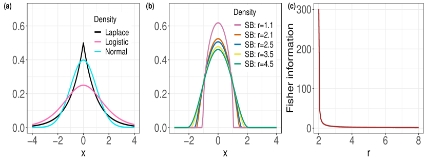
Figure 1: (a) Plot of the standard Laplace, standard normal and standard logistic densities. (b) Plot of the symmetrized beta density $f_{0,r}$, defined in (15), for different values of $r$. (c) Plot of Fisher information $\mathcal{I}_{f_{0,r}}$ vs $r$ where $f_{0,r}$ is the symmetrized beta density.

This section compares the efficiency of our estimators and the coverage of the resulting confidence intervals with that of Stone and Beran. The general set-up of the simulation is as follows. We consider as $g_{0}$ the standard normal, standard logistic, and standard Laplace density. We also consider a fourth density, namely the symmetrized beta density, which is defined as follows:

$$f_{0}(x)\equiv f_{0,r}(x)=\dfrac{\Gamma\bigg{(}(3+r)/2\bigg{)}}{\sqrt{\pi r}\Gamma(1+r/2)}\bigg{(}1-\dfrac{x^{2}}{r}\bigg{)}^{r/2}1_{[-\sqrt{r},\sqrt{r}]}(x),\quad r>0.$$ (15)

Here $\Gamma$ is the usual Gamma function. It is straightforward to verify that in this case

$$\phi_{0}^{\prime}(x)=\dfrac{-x}{1-x^{2}/r}1_{[-\sqrt{r},\sqrt{r}]}(x)\quad\text{and }\quad\phi_{0}^{\prime\prime}(x)=-\frac{(1+x^{2}/r)}{(1-x^{2}/r)^{2}}1_{[-\sqrt{r},\sqrt{r}]}(x).$$

Some computation shows that $r\leq 2$ leads to $\mathcal{I}_{f_{0,r}}=\infty.$ However for $r>2$, $\mathcal{I}_{f_{0,r}}<\infty$, and $f_{0}\in\mathcal{P}_{0}$. This is an example of a case where Assumption A fails to hold because $\phi_{0}^{\prime\prime}$ is unbounded. We consider the symmetrized beta density with $r=2.1$ and $4.5$.

See Figure 1a and 1b for a pictorial representation of the above-mentioned densities. Figure 1c displays the plot of $\mathcal{I}_{f_{0,r}}$ versus $r$ for the symmetrized beta density, which depicts that $\mathcal{I}_{f_{0,r}}$ decreases steeply for $r>2$. This finding is consistent with $\mathcal{I}_{f_{0}}$ being $\infty$ when $f_{0}$ is the uniform density on $[-1,1].$

We set $\theta_{0}=0$, and generate $3000$ samples of size $n=30$, $100$, $200$, and $500$ from each of the above-mentioned densities. We define the efficiency of an estimator $\theta_{n}$ by

$$\text{Efficiency}(\theta_{n})=\dfrac{1/(n\mathcal{I}_{f_{0}})}{Var(\theta_{n})}.$$ (16)

In practice, we replace $Var(\theta_{n})$ by its Monte Carlo estimate.

The shape-constrained estimators:

Along with the MLE and the untruncated one step estimator defined in (5), we consider the truncated one step estimators with truncation level $\eta=10^{-2}$, $10^{-3}$, and $10^{-5}$. We select the sample mean as the preliminary estimator $\bar{\theta}_{n}$ because it exhibited slightly better overall performance than other potential choices of $\bar{\theta}_{n}$, e.g. the median and the trimmed mean. We choose the partial MLE estimator and the smoothed symmetrized estimator $\tilde{g}_{n}^{sym,sm}$ as the estimator of $g_{0}$ because simulations suggest that they perform significantly better than $\tilde{g}_{n}^{geo,sym}$.

Comparators: Stone and Beran’s estimators:

As mentioned earlier, Stone’s estimator is a truncated one step estimator which uses symmetrized Gaussian kernels to estimate $g_{0}$. Similar to Stone, we let the corresponding truncation parameter and the kernel bandwidth parameter to be $d_{n}s_{n}$ and $t_{n}s_{n}$, respectively, where $s_{n}$ is the median absolute deviation (MAD), and $d_{n}>0$ and $t_{n}>0$ are tuning parameters. Following Stone, we take the preliminary estimator to be the sample median.

As previously stated, Beran’s estimator is a rank-based estimator which depends on the scores. Beran uses Fourier series expansion to estimate the scores, which requires choosing (a) the number of basis functions ($b_{c,n}$), and (b) a scaling parameter $\rho_{n}$, which is used to approximate a derivative term by quotients during the estimation of the Fourier coefficients of the score. This estimator uses a preliminary estimator of $\theta$, which we take to be the sample median following Beran’s suggestion. In this case, the sum of squares of the estimated Fourier coefficients is a consistent estimator of $\mathcal{I}_{f_{0}}$ (see (3.3) of Beran, 1974).

For sample size $n=40$, Stone uses $d_{n}=20$ and $t_{n}=0.60$, but Beran does not give any demonstration on how to choose the tuning parameters. To choose some reliable values for the associated tuning parameters, we start with some pre-selected grids, and employ a grid search procedure (see Appendix H for more details). The selected tuning parameter is the maximizer of the estimated efficiency among the grid, where the efficiency is estimated using one hundred Monte Carlo replications. Of course, this procedure requires the knowledge of the unknown distribution, and hence, not implementable in practice. However, our procedure at least guarantees a reliable benchmark to compare the performance of our estimators. We refer to the resulting tuning parameters as “optimal” for the sake of simplicity. However, it should be kept in mind that these tuning parameters depend on the chosen grid, and therefore, may be different from the globally optimal tuning parameters if the grid selection is not accurate enough. This could have been overcome by an exhaustive search but that is beyond the scope of the current paper.

For each distribution and each sample size, we construct two versions of the nonparametric estimators. The first version is based on the aforementioned optimal tuning parameter, and the other version uses tuning parameters slightly away from the optimal region. For convenience, we will refer to the second set of tuning parameters as “non-optimal”. See Appendix H for more details on these tuning parameters.

We should mention that neither Stone nor Beran construct confidence intervals. However, both estimators rely on consistent estimators of $\mathcal{I}_{f_{0}}$, namely, the estimator $\widehat{A}_{n}(r_{n},c_{n})$ of Stone (see (1.10) of Stone), and the squared $L_{2}$ norm of the estimated score in Beran. We use the above estimators of $\mathcal{I}_{f_{0}}$ to build the respective confidence intervals of Stone and Beran.

Results:

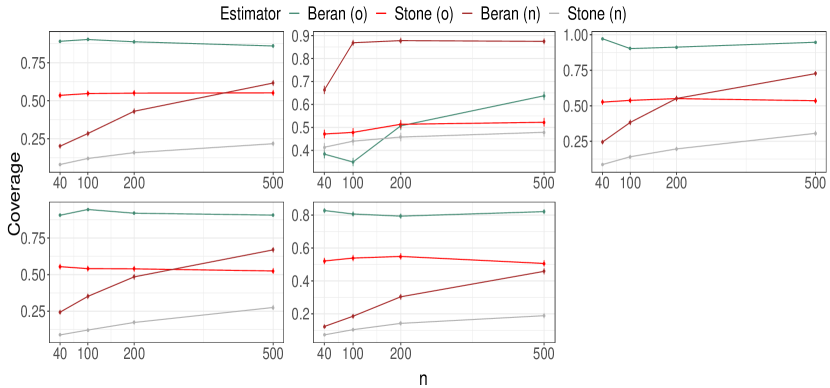
Figure 5: Comparison of the coverage of the 95% confidence intervals for Beran’s and Stone’s estimators: the data-generating distributions are normal (topleft), Laplace (topmiddle), Symmetrized beta with $r=2.1$ (topright), and $r=4.5$ (bottomleft), and logistic (bottommiddle). Here (o) stands for the optimal tuning parameter, and (n) corresponds to the non-optimal tuning parameter. The errorbars are given by $\pm 2$ standard deviation.

Figure 2 implies that Stone and Beran’s estimators have high efficiency when they are equipped with the optimal tuning parameters. In fact Stone’s estimator has better efficiency than all other estimators in case of logistic and normal distribution. However, even with the optimal tuning parameter, the coverage of Stone’s confidence interval is quite low (see Figure 5). The coverage of Beran’s confidence interval is comparatively better but still not as good as the shape-constrained estimators (see Figure 3). The poor coverage of the nonparametric confidence intervals is probably due to their smaller width, as shown by Figure 4. We suspect that for our tuning parameters, the nonparametric estimators of $\mathcal{I}_{f_{0}}$ overestimate $\mathcal{I}_{f_{0}}$, leading to narrow confidence intervals. When the tuning parameters are non-optimal, the nonparametric estimators suffer in terms of both efficiency and the coverage. This is most evident in large samples because in this case, their performance does not significantly improve with the sample size. Figure 2 and 3 entail that all estimators have markedly poor performance in the symmetrized beta case when $r=2.1$.

Let us turn our attention to the one step estimators now. Figure 2 underscore that the efficiency of the one step estimators monotonously decreases with the truncation, with the highest efficiency being observed at the truncation level zero. However, the difference becomes smaller as the truncation level decreases. In particular, at truncation level $10^{-5}$, the difference almost vanishes. The one step estimators with lower truncation level, i.e. $\eta\leq 0.001$, exhibit satisfactory performance in terms of both efficiency and coverage (see Figure 2 and Figure 3). The estimators with higher truncation level lag in terms of efficiency as expected, although they exhibit superior coverage in some cases.

The additional gain in coverage that sometimes accompany higher levels of truncation is probably due to slightly wider confidence intervals (see Figure 4). Wider confidence intervals are expected with high levels of truncation since the length of the confidence intervals, which is a constant multiple of $\widehat{\mathcal{I}}_{n}(\eta)^{-1}$, increases in $\eta$. However, higher level of truncation may not always lead to a better coverage, especially since high truncation level can also result in significant loss of efficiency. See for instance the case of symmetrized beta with $r=2.1$, where the one step estimators with truncation $0.01$ lags behind the other one-step estimators in terms of both efficiency and coverage. This case clearly demonstrates that the one step estimators with higher level of truncation are not always reliable. In contrast, the one step estimators with low level of truncation, particularly the untruncated one step estimator, always exhibit satisfactory performance. In view of above, we propose the untruncated estimator for practical implementation.

Close inspection shows the smoothed symmetrized estimators have better overall performance than the partial MLE estimators with the obvious exception of Laplace distribution, which has a non-smooth density. Finally, we note that the one step estimators with lower truncation level have better efficiency than the MLE under all distributions except Laplace. However, when it comes to the coverage of the confidence intervals, the MLE can be competitive with the best one step estimators, especially in small samples.

In summary, the coverage of the nonparametric confidence intervals is not satisfactory for the tuning parameters considered here, and the efficiency of the nonparametric estimators depends crucially on the tuning parameters. For some choices of tuning parameter, these estimators may exhibit excellent efficiency but for other choices, they severely underperform. In contrast, our untruncated one step estimator and the resulting confidence interval perform reasonably well under all scenarios. The performance of the untruncated one-step estimator also speaks in favor of our conjecture that it is an adaptive estimator. Although we do not show the plots of the mean squared error (MSE) here, they depict the same patterns as the efficiency plots in Figure 2.

We close this section with a remark on the necessity of Assumption A. The symmetrized beta distributions do not satisfy Assumption A, but the one step estimators still seem to be efficient when $r=4.5$. Although the one step estimators perform poorly in case of $r=2.1$, they still perform better than Stone and Beran’s estimators, whose asymptotically efficiency under this distribution is theoretically validated. Thus, our simulations do not refute the possibility that Assumption A might be unnecessary.

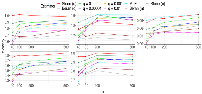
(a) Comparison plot when the one step estimators are the Partial MLE estimator

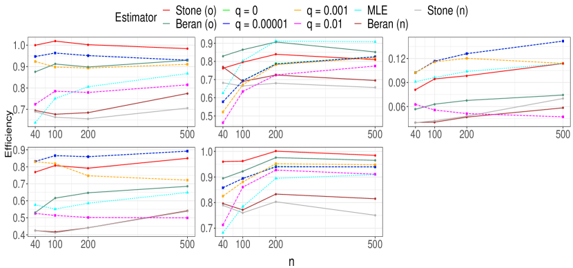
(b) Comparison plot when the one step estimators are the smoothed symmetrized estimator

Figure 2: comparison of efficiency: the data-generating distributions are normal (topleft), Laplace (topmiddle), Symmetrized beta with $r=2.1$ (topright), and $r=4.5$ (bottomleft), and logistic (bottommiddle). For Stone’s and Beran’s estimators (in solid lines), (o) stands for the optimal tuning parameter, and (n) corresponds to the non-optimal tuning parameter. Here $q$ stands for the truncation parameter $\eta$ in our one-step estimators (in dashed lines).

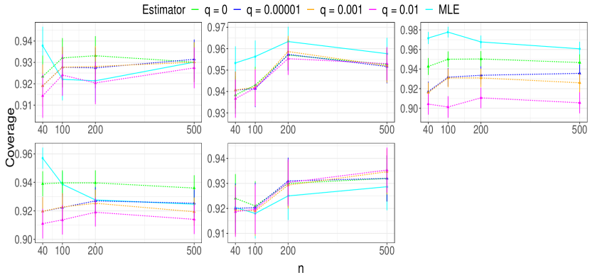
(a) Comparison plot when the one step estimators are the Partial MLE estimator

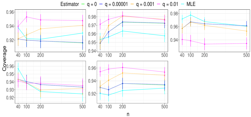
(b) Comparison plot when the one step estimators are the smoothed symmetrized estimator

Figure 3: Comparison of the coverage of the 95% confidence intervals: the data-generating distributions are normal (topleft), Laplace (topmiddle), Symmetrized beta with $r=2.1$ (topright), and $r=4.5$ (bottomleft), and logistic (bottommiddle). Here $q$ stands for the truncation parameter $\eta$ in our one-step estimators. The errorbars are given by $\pm 2$ standard deviation.

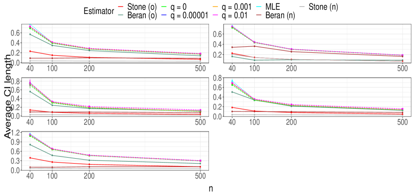
(a) Comparison plot when the one step estimators are the Partial MLE estimator

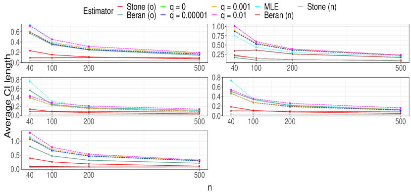
(b) Comparison plot when the one step estimators are the smoothed symmetrized estimator

Figure 4: Comparison of the average confidence interval length (averaged across the 3000 Monte Carlo samples): the data-generating distributions are normal (topleft), Laplace (topmiddle), Symmetrized beta with $r=2.1$ (topright), and $r=4.5$ (bottomleft), and logistic (bottommiddle). For Stone’s and Beran’s estimators (in solid lines), (o) stands for the optimal tuning parameter, and (n) corresponds to the non-optimal tuning parameter. Here $q$ stands for the truncation parameter $\eta$ in our one-step estimators (in dashed lines). The errorbars are given by $\pm 2$ standard deviation.

5 Discussion

In this paper, we show that under the additional assumption of log-concavity, adaptive estimation of $\theta_{0}$ is possible with only one tuning parameter. Our simulations suggest that the tuning parameter-free untruncated one step estimator may also be adaptive. This demonstrates the usefulness of log-concavity assumption in semiparametric models in facilitating a simplified estimation procedure. It is natural to ask what happens if the above shape restriction fails to hold. For functionals of log-concave MLE type estimators, this question can be partially answered building on the log-concave projection theory developed by Dümbgen et al. (2011), Cule and Samworth (2010), Xu and Samworth (2019), and Barber and Samworth (2020). See Laha (2019) for discussion of the case when the log-concavity assumption is violated in our model $\mathcal{P}_{0}$. In particular, it can be shown that, even if $f\notin\mathcal{P}_{0}$, as long as $f$ is symmetric about $\theta_{0}$, the MLE and the truncated one step estimators are still consistent under mild conditions.

Appendix

The appendix is organized as follows. Appendices A, B, and C contain the proofs for the one step estimators, where Appendices D, E, and F contain the proofs for the MLE. The proof of the main theorem is presented first, followed by the auxiliary lemmas required for the proof. Some common technical facts, which are used repeatedly in the proofs, are listed at the end in Appendix G. Appendix H contains details on the selected tuning parameters for Stone and Beran’s estimators.

Before proceeding any further, we introduce some new notations and terminologies. For $i=1,\ldots,n$, consider the pseudo-observations $Z_{i}=X_{i}-\theta_{0}$. Note that, if the $X_{i}$’s have density $f_{0}$, then the $Z_{i}$’s have density $g_{0}$, and distribution function $G_{0}$. We will denote the log-densities corresponding to ${\widehat{h}_{n}^{sm}}$, $\tilde{g}_{n}^{sym,sm}$, $\widehat{g}_{\theta}$ and ${\tilde{g}_{n}}^{geo,sym}$ by $\tilde{\phi}_{n}^{sm}$, $\tilde{\psi}_{n}^{sym,sm}$, $\widehat{\psi}_{\theta}$ and $\tilde{\psi}_{n}^{geo,sym}$, respectively. As usual, $(\tilde{\phi}_{n}^{sm})^{\prime}$, $(\tilde{\psi}_{n}^{sym,sm})^{\prime}$, $\widehat{\psi}_{\theta}^{\prime}$, and $(\tilde{\psi}_{n}^{geo,sym})^{\prime}$ will denote the corresponding right derivatives. We remark in passing that there is nothing special about the right derivative, and any $L_{1}$ derivative would have worked. However, we fix one specific version to avoid future confusion. We denote the distribution functions of ${\widehat{h}_{n}^{sm}}$, $\tilde{g}_{n}^{sym,sm}$, and ${\tilde{g}_{n}}^{geo,sym}$ by $\widehat{H}_{n}^{sm}$, $\tilde{G}^{sym,sm}_{n}$, and $\tilde{G}_{n}^{geo,sym}$, respectively.

The empirical process of the $X_{i}$’s will be denoted by $\mathbb{G}_{n}=\sqrt{n}(\mathbb{F}_{n}-F_{0})$. For any function $h:\mathbb{R}\mapsto\mathbb{R}$, and a measure $Q$ on $\mathbb{R}$, we write $Qh:=\int_{\mathbb{R}}hdQ$ provided $h$ is integrable with respect to $Q$. Suppose $\mathcal{H}$ is a class of $Q$-measurable functions. We denote by $\|Q\|_{\mathcal{H}}$ the supremum $\sup_{h\in\mathcal{H}}\absolutevalue{Qh}$. For the sake of simplicity, we will denote $\tilde{\delta}_{n}=\theta_{0}-\bar{\theta}_{n}$ and $\delta_{n}=\theta_{0}-\widehat{\theta}_{n}$ in our proofs.

For a measure $P$ on $\mathbb{R}$, we define the $L_{P,k}$ norm of the function $h$ as

$$\|h\|_{P,k}=\bigg{(}\displaystyle\int_{-\infty}^{\infty}|h(x)|^{k}dP(x)\bigg{)}^{1/k},\quad k\geq 1.$$

For any class of functions $\mathcal{H}$, we will denote

$$\|\mathcal{H}\|_{P,k}=\sup_{h\in\mathcal{H}}\|h\|_{P,k}.$$

For two distribution functions $F_{1}$ and $F_{2}$ with densities $f_{1}$ and $f_{2}$, the total variation distance between $F_{1}$ and $F_{2}$ is given by $d_{TV}(F_{1},F_{2})=\|f_{1}-f_{2}\|_{1}/2$. We define the Wasserstein distance between two measures $\mu$ and $\nu$ on $\mathbb{R}$ by

$$d_{W}(\mu,\nu)=\displaystyle\int_{-\infty}^{\infty}|F(x)-G(x)|dx,$$ (17)

where $F$ and $G$ are the distribution functions corresponding to $\mu$ and $\nu$ respectively. This representation of $d_{W}(\mu,\nu)$ follows from Villani (2003), page $75$. By an abuse of notation, sometime we will denote the above distance by $d_{W}(F,G)$ as well. Suppose $\epsilon>0$. For any class of functions $\mathcal{H}$ and a norm $\|\cdot\|$, the bracketing entropy $N_{[\ ]}(\epsilon,\mathcal{H},\|\cdot\|)$ is as in Definition 2.1.6, page 83 of Van der Vaart and Wellner (1996). The covering number $N(\epsilon,\mathcal{H},\|\cdot\|)$ is as defined in page 83 of Van der Vaart and Wellner (1996).

For two sets $A$ and $B$, $A\times B$ will represent the Cartesian product. For any set $A\subset\mathbb{R}$, and $x\in\mathbb{R}$, we use the usual notation $A+x$ to denote the translated set $\{y+x\ :\ y\in A\}$. The notation $\overline{A}$ will refer to the closure of the set $A$. For any function $h$, $1_{[h(x)\leq C]}$ will denote the indicator function of the event $h(x)\leq C$. For any set $A$, we let $1_{A}(x)$ be the indicator function of the event $x\in A$. As usual, we denote by $\varphi$ the standard Gaussian density.

In some of our proofs, we will replace $\tilde{g}_{n}^{sym,sm}$ by a more general mixture density which satisfies Condition 3.

Condition 3 (Condition for $\tilde{g}_{n}^{sym,sm}$).

The density $\tilde{g}_{n}$ is symmetric about zero and satisfies $\tilde{g}_{n}(x)=(g_{1n}(x)+g_{2n}(x))/2$, where $g_{1n}$ and $g_{2n}$ are log-concave densities. The densities $\tilde{g}_{n}$, $g_{1n}$, and $g_{2n}$ satisfy Conditions 1 and 2. Moreover, $\text{supp}(g_{1n})=\text{supp}(g_{2n})=\mathbb{R}$, and the $p$ in Condition 2 is the same for $\tilde{g}_{n}$, $g_{1n}$, and $g_{2n}$.

We will later show in Lemma B.1 that ${\widehat{h}_{n}^{sm}}(\bar{\theta}_{n}\pm\mathord{\cdot})$ and $\tilde{g}_{n}^{sym,sm}$ satisfy Condition 1, and in Lemma C.1, we will show that these densities satisfy Condition 2 with $p=1/5$. Since ${\widehat{h}_{n}^{sm}}(\bar{\theta}_{n}\pm\mathord{\cdot})$ is the convolution of two log-concave densities, it is log-concave. That $\tilde{g}_{n}^{sym,sm}$ satisfies Condition 3 follows immediately from the above results.

We will frequently use the fact that if $f$ is a log-concave density, then $f>0$ on $J(F)=\{x\in\mathbb{R}:0<F(x)<1\}$ (cf. Theorem 1(iv) of Dümbgen et al., 2017). Therefore, $\mathrm{int}(\mathrm{dom}(\log f))=\mathrm{int}(\text{supp}(f))=\mathrm{int}(J(F))$. As a consequence, $F^{-1}$ is strictly increasing, and differentiable with derivative $1/f(F^{-1}(t))$ on $(0,1)$ by Fact 8. Also, a log-concave $f$ is thus continuous on $\mathrm{int}(J(F))$ by Theorem 10.1 of Rockafellar (1970). When $f_{0}\in\mathcal{P}_{0}$, furthermore, $f_{0}$ and $g_{0}$ are absolutely continuous on $\mathbb{R}$ by Theorem 3 of Huber (1964). Now we list below some useful facts about log-concave densities.

Fact 1 (Lemma 1 of Cule and Samworth (2010)).

If $f$ is a univariate log-concave density, then there exists $\alpha>0$ and $\beta\in\mathbb{R}$ so that $f(x)\leq e^{-\alpha|x|+\beta}$.

Fact 2.

If $f$ is log-concave, then $f/F$ is non-increasing on $J(F)$ and $f/(1-F)$ is non-decreasing on $J(F)$.

Proof.

This is a well known fact about log-concave densities. See Theorem 1 and Corollary 2 of Bagnoli and Bergstrom (2005) or Dümbgen et al. (2017). ∎

The following two facts will be very useful to lower bound $\tilde{g}_{n}$ on $[-\xi_{n},\xi_{n}]$.

Fact 3.

Suppose $\tilde{g}_{n}$ is a log-concave density satisfying Condition 1. Then for any $x\in\mathbb{R}$,

$$\tilde{g}_{n}(x)\geq\omega_{n}\min(\tilde{G}_{n}(x),1-\tilde{G}_{n}(x)),$$

where $\omega_{n}\geq 0$ satisfies $\omega_{n}\to_{p}\omega_{0}>0$. Here $\omega_{0}>0$ is a constant depending only on $g_{0}$.

Proof.

If $\tilde{G}_{n}(x)$ is zero or one, then the statement trivially holds. Therefore, we assume $x\in J(\tilde{G}_{n})$, i.e. $0<\tilde{G}_{n}(x)<1$. For $q\in(0,1/2)$, Fact 2 implies

$$\tilde{g}_{n}(\tilde{G}_{n}^{-1}(q))\geq 2q\Big{(}\tilde{g}_{n}(\tilde{G}_{n}^{-1}(1/2))\Big{)}\geq 2\min(q,1-q)\tilde{g}_{n}(\tilde{G}_{n}^{-1}(1/2)).$$

On the other hand, for $q\in(1/2,1)$, Fact 2 implies

$$\tilde{g}_{n}(\tilde{G}_{n}^{-1}(q))\geq 2(1-q)\tilde{g}_{n}(\tilde{G}_{n}^{-1}(1/2))\geq 2\min(q,1-q)\tilde{g}_{n}(\tilde{G}_{n}^{-1}(1/2)).$$

Because $\tilde{G}_{n}(x)\in(0,1)$, replacing $q$ by $\tilde{G}_{n}(x)$ we obtain that

$$\tilde{g}_{n}(x)\stackrel{{\scriptstyle(a)}}{{=}}\tilde{g}_{n}(\tilde{G}_{n}^{-1}(\tilde{G}_{n}(x)))\geq 2\tilde{g}_{n}(\tilde{G}_{n}^{-1}(1/2))\min\Big{(}\tilde{G}_{n}(x),1-\tilde{G}_{n}(x)\Big{)}.$$ (18)

Here (a) uses the fact that $\tilde{g}_{n}(x)>0$ which follows since $x\in\mathrm{int}(J(\tilde{G}_{n}))=\mathrm{int}(\mathrm{dom}(\tilde{\psi}_{n}))$. The rest of the proof follows setting $\omega_{n}=2\tilde{g}_{n}(\tilde{G}_{n}^{-1}(1/2))$, which converges in probability to $\omega_{0}=2g_{0}(0)$ by Condition 1 and Fact 11.

∎

Fact 4.

Suppose either $\tilde{g}_{n}$ satisfies Condition 3, or $\tilde{g}_{n}$ is a log-concave density satisfying Condition 1. Then the assertions of Fact 3 hold.

Proof.

If $\tilde{g}_{n}\in\mathcal{LC}$, the proof follows from Fact 3. Therefore we consider the case when $\tilde{g}_{n}$ satisfies Condition 3. Since the component densities $g_{1n}$ and $g_{2n}$ in Condition 3 are log-concave, Fact 3 applies to them. Denote by $G_{1n}$ and $G_{2n}$ the corresponding distribution functions. Equation 18 in the proof of Fact 3 implies

$$g_{1n}(x)+g_{2n}(x)\geq b_{n}\bigg{\{}G_{1n}(x)\Big{(}1-G_{1n}(x)\Big{)}+G_{2n}(x)\Big{(}1-G_{2n}(x)\Big{)}\bigg{\}},$$

where

$$b_{n}=2\min\bigg{(}g_{1n}(G_{1n}^{-1}(1/2)),g_{2n}(G_{2n}^{-1}(1/2))\bigg{)}\to_{p}2g_{0}(0)$$

by the fact that $g_{1n}$ and $g_{2n}$ satisfy Condition 1 and Fact 11. Fact 16 implies that

$$G_{1n}(x)\Big{(}1-G_{1n}(x)\Big{)}+G_{2n}(x)\Big{(}1-G_{2n}(x)\Big{)}$$

$$\geq \ \min\bigg{(}\frac{G_{1n}(x)+G_{2n}(x)}{2},1-\frac{G_{1n}(x)+G_{2n}(x)}{2}\bigg{)}$$

$$= \ \min(\tilde{G}_{n}(x),1-\tilde{G}_{n}(x)),$$

where $\tilde{G}_{n}$ is the distribution function corresponding to $\tilde{g}_{n}=(g_{1n}+g_{2n})/2$. Letting $\omega_{n}=b_{n}/2$, we have

$$\tilde{g}_{n}(x)\geq\frac{b_{n}}{2}\min(\tilde{G}_{n}(x),1-\tilde{G}_{n}(x)),$$

which completes the proof. ∎

Appendix A Proof of Theorem 1

We first argue that it suffices to prove the theorem only for the case when $\eta_{n}$ equals $Cn^{-2p/5}$. In the latter case, we would show $\sqrt{n}(\tilde{\theta}_{n}-\theta_{0})\to_{d}N(0,\mathcal{I}_{f_{0}}^{-1})$ for $\eta_{n}=Cn^{-2p/5}$ when $H(\tilde{g}_{n},g_{0})=O_{p}(n^{-p})$. Note that for any $p^{\prime}\in(0,p]$, $H(\tilde{g}_{n},g_{0})=O_{p}(n^{-p^{\prime}})$ trivially holds since $H(\tilde{g}_{n},g_{0})=O_{p}(n^{-p})$. Therefore, replacing $p$ by $p^{\prime}$ in what we just proved, $\sqrt{n}(\tilde{\theta}_{n}-\theta_{0})\to_{d}N(0,\mathcal{I}_{f_{0}}^{-1})$ would follow identically for $\eta_{n}=Cn^{-2p^{\prime}/5}$. Thus, it is enough to consider the case when $\eta_{n}=Cn^{-2p/5}$.

From (7) we obtain that

$$-(\tilde{\theta}_{n}-\bar{\theta}_{n})=\displaystyle\int_{\bar{\theta}_{n}-\xi_{n}}^{\bar{\theta}_{n}+\xi_{n}}\dfrac{\tilde{\psi}_{n}^{\prime}(x-\bar{\theta}_{n})}{\widehat{\mathcal{I}}_{n}(\eta_{n})}d\mathbb{F}_{n}(x)=\displaystyle\int_{-\xi_{n}}^{\xi_{n}}\dfrac{\tilde{\psi}_{n}^{\prime}(z)}{\widehat{\mathcal{I}}_{n}(\eta_{n})}d\mathbb{F}_{n}(z+\bar{\theta}_{n}).$$

Denoting $\tilde{\delta}_{n}=\theta_{0}-\bar{\theta}_{n}$, we observe that the above expression writes as

$$\underbrace{\displaystyle\int_{-\xi_{n}}^{\xi_{n}}\dfrac{\tilde{\psi}^{\prime}_{n}(z)-{\psi}_{0}^{\prime}(z-\tilde{\delta}_{n})}{\widehat{\mathcal{I}}_{n}(\eta_{n})}d(\mathbb{F}_{n}(z+\bar{\theta}_{n})-F_{0}(z+\bar{\theta}_{n}))}_{T_{1n}}$$

$$\ +\underbrace{\displaystyle\int_{-\xi_{n}}^{\xi_{n}}\dfrac{\tilde{\psi}^{\prime}_{n}(z)}{\widehat{\mathcal{I}}_{n}(\eta_{n})}\bigg{(}f_{0}(z+\bar{\theta}_{n})-g_{0}(z)\bigg{)}dz}_{T_{2n}}+\underbrace{\displaystyle\int_{-\xi_{n}}^{\xi_{n}}\dfrac{\tilde{\psi}^{\prime}_{n}(z)-{\psi}_{0}^{\prime}(z)}{\widehat{\mathcal{I}}_{n}(\eta_{n})}g_{0}(z)dz}_{T_{3n}}$$

$$\ +\underbrace{\displaystyle\int_{-\xi_{n}}^{\xi_{n}}\dfrac{{\psi}_{0}^{\prime}(z)}{\widehat{\mathcal{I}}_{n}(\eta_{n})}g_{0}(z)dz}_{T_{4n}}+\underbrace{\displaystyle\int_{-\xi_{n}}^{\xi_{n}}\dfrac{{\psi}_{0}^{\prime}(z-\tilde{\delta}_{n})}{\widehat{\mathcal{I}}_{n}(\eta_{n})}d(\mathbb{F}_{n}(z+\bar{\theta}_{n})-F_{0}(z+\bar{\theta}_{n}))}_{T_{5n}}$$ (19)

Observe that $T_{3n}$ and $T_{4n}$ vanish since $\tilde{\psi}^{\prime}_{n}$ and $\psi^{\prime}_{0}$ are odd functions while $g_{0}$ is an even function.

The proof of Theorem 1 has three main steps. The first step uses Donsker Theorem to show that the empirical process term $T_{1n}$ is $o_{p}(n^{-1/2})$. The term $T_{2n}$ accounts for the bias due to the use of $\bar{\theta}_{n}$ instead of the true center $\theta_{0}$ in the construction of the scores. The second step of the proof shows that the order of $T_{2n}$ is same as $\tilde{\delta}_{n}=\theta_{0}-\bar{\theta}_{n}$. In particular, we will show that $T_{2n}=-\tilde{\delta}_{n}(1+o_{p}(1))$. Since $\tilde{\delta}_{n}=O_{p}(n^{-1/2})$, the above two steps lead to

$$\sqrt{n}(\bar{\theta}_{n}-\tilde{\theta}_{n})=o_{p}(1)+\sqrt{n}(\bar{\theta}_{n}-\theta_{0})+\sqrt{n}T_{5n}.$$

The third step of the proof shows that the term $\sqrt{n}T_{5n}$ is asymptotically normal with variance $\mathcal{I}_{f_{0}}^{-1}$. A rearrangement of the terms in the above display then establishes the desired asymptotic convergence of $\sqrt{n}(\tilde{\theta}_{n}-\theta_{0})$. The rest of the proof is devoted to proofs of the above-mentioned three steps.

First step: asymptotic negligibility of $\sqrt{n}T_{1n}$:

First, let us denote $\mathcal{T}_{n}=[\bar{\theta}_{n}-\xi_{n},\bar{\theta}_{n}+\xi_{n}]$. Recall that in Section 1.1 we denoted the empirical process $\sqrt{n}(\mathbb{F}_{n}-F_{0})$ by $\mathbb{G}_{n}$. Note that $\sqrt{n}T_{1n}$ also writes as

$$\sqrt{n}T_{1n}=\sqrt{n}\displaystyle\int_{\bar{\theta}_{n}-\xi_{n}}^{\bar{\theta}_{n}+\xi_{n}}\dfrac{\tilde{\psi}^{\prime}_{n}(x-\bar{\theta}_{n})-{\phi}_{0}^{\prime}(x)}{\widehat{\mathcal{I}}_{n}(\eta_{n})}d(\mathbb{F}_{n}-F_{0})(x)=\displaystyle\int_{-\infty}^{\infty}\dfrac{h_{n}(x)}{\widehat{\mathcal{I}}_{n}(\eta_{n})}d\mathbb{G}_{n}(x),$$ (20)

where by $h_{n}$ we denote the function

$$h_{n}(x)=(\tilde{\psi}^{\prime}_{n}(x-\bar{\theta}_{n})-\phi_{0}^{\prime}(x))1_{\mathcal{T}_{n}}(x),\quad x\in\mathbb{R}.$$ (21)

Because $\eta_{n}=O(n^{-2p/5})$, Lemma A.15 implies

$$\sup_{x\in\mathcal{T}_{n}}|\tilde{\psi}_{n}^{\prime}(x-\bar{\theta}_{n})|=O_{p}(n^{p/5}).$$ (22)

Thus $\tilde{\psi}_{n}^{\prime}$ restricted to the compact set $\mathcal{T}_{n}$ is bounded. We can extend the function $x\mapsto\tilde{\psi}_{n}^{\prime}(x)1_{\mathcal{T}_{n}}(x)$ to $\mathbb{R}$ in a way such that the resulting function $\widehat{u}_{n}$ is still monotone and has the same bound. This can be done by setting $\widehat{u}_{n}$ to be $\tilde{\psi}_{n}^{\prime}(\bar{\theta}_{n}-\xi_{n})$ and $\tilde{\psi}_{n}^{\prime}(\bar{\theta}_{n}+\xi_{n})$ on the intervals $(-\infty,\bar{\theta}_{n}-\xi_{n}]$ and $[\bar{\theta}_{n}+\xi_{n},\infty)$, respectively. Note also that we can replace $\tilde{\psi}_{n}^{\prime}$ by $\widehat{u}_{n}$ in the definition of $h_{n}$, i.e.

$$h_{n}(x)=(\widehat{u}_{n}(x-\bar{\theta}_{n})-{\phi}_{0}^{\prime}(x))1_{\mathcal{T}_{n}}(x).$$ (23)

Let us denote $M_{n}=Cn^{p/5}$ for some $C>0$ and define

$$\mathcal{U}_{n}(M_{n})=\bigg{\{}u:\mathbb{R}\mapsto[-M_{n},M_{n}]\ \bigg{|}\ \ u\text{ is non-increasing}\bigg{\}}.$$ (24)

Since $\|\widehat{u}_{n}\|_{\infty}=O_{p}(n^{p/5})$, for sufficiently large $C$, $\hat{u}_{n}(\mathord{\cdot}-\bar{\theta}_{n})\in\mathcal{U}_{n}(M_{n})$ with high probability. Now define the class $\mathcal{H}_{n}(C)$ by

$$\mathcal{H}_{n}(C)=\bigg{\{}h:\mathbb{R}\mapsto\mathbb{R}\ \bigg{|}\ \ h(x)=(u(x)-{\phi}_{0}^{\prime}(x))1_{[r_{1},r_{2}]}(x),\ u\in\mathcal{U}_{n}(M_{n}),$$

$$\ \|h\|_{P_{0},2}\leq Cn^{-2p/5}(\log n)^{3},\ \ \|h\|_{\infty}\leq M_{n},$$

$$\ [r_{1},r_{2}]\subset[\theta_{0}-C\log n,\theta_{0}+C\log n]\cap\mathrm{int}(\mathrm{dom}(\phi_{0}))\bigg{\}}.$$

The notation $\mathcal{H}_{n}(C)$ does not depend on $M_{n}$ because $M_{n}=Cn^{p/5}$ is also a function of $C$.

We want to show that $h_{n}\in\mathcal{H}_{n}(C)$ with high probability for large $n$. Note that

$$\sup_{x\in\mathcal{T}_{n}}|\phi^{\prime}_{0}(x)|=\sup_{x\in[-\delta_{n}-\xi_{n},-\delta_{n}+\xi_{n}]}|\psi^{\prime}_{0}(x)|.$$

Lemma A.10 in conjunction with the fact that $\eta_{n}=O(n^{-2p/5})$ implies

$$\sup_{x\in\mathcal{T}_{n}}|\phi_{0}^{\prime}(x)|=O_{p}(\log n).$$ (25)

Thus (22) and (25) imply $\|h_{n}\|_{\infty}=O_{p}(n^{p/5})$. Lemma A.16 bounds the $L_{P_{0},2}$ norm of $h_{n}$ entailing $\|h_{n}\|_{P_{0},2}=O_{p}(n^{-2p/5}(\log n)^{3})$. Lemma A.6 implies, on the other hand,

$$\lim_{n\to\infty}P\Big{(}\mathcal{T}_{n}\subset[\theta_{0}-C\log n,\theta_{0}+C\log n]\cap\mathrm{int}(\mathrm{dom}(\phi_{0}))\Big{)}=1.$$

Therefore, we conclude that given $t>0$, we can choose $C>0$ so large such that $P(h_{n}\in\mathcal{H}_{n}(C))>1-t$.

Theorem 2.7.5 of Van der Vaart and Wellner (1996) (pp. $159$) states that there exists an absolute constant $C^{\prime}>0$ so that for any $\epsilon>0$ and any probability measure $\mathbb{R}$ on the real line,

$$\log N_{[\ ]}(\epsilon,\mathcal{U}_{n}(M_{n}),L_{2}(Q))\leq C^{\prime}M_{n}\epsilon^{-1}.$$ (26)

On the other hand, using Theorem 2.7.5 of Van der Vaart and Wellner (1996), it can also be shown that the class $\mathcal{F}_{I}$ of all indicator functions of the form $1_{[z_{1},z_{2}]}$, where $z_{1}\leq z_{2}$ with $z_{1},z_{2}\in\mathbb{R}$, satisfies

$$\log N_{[\ ]}(\epsilon,\mathcal{F}_{I},L_{2}(Q))\leq C^{\prime}2\epsilon^{-1}.$$ (27)

Using (26) and (27) we derive that

$$\log N_{[\ ]}(\epsilon,\mathcal{H}_{n}(C),L_{2}(P_{0}))\lesssim{M_{n}}{\epsilon}^{-1}.$$

For $x<1$, the bracketing integral

$$\mathcal{J}_{[\ ]}(x,\mathcal{H}_{n}(C),L_{2}(P_{0}))= \ \displaystyle\int_{0}^{x}\sqrt{1+\log N_{[\ ]}(\epsilon,\mathcal{H}_{n}(C),L_{2}(P_{0}))}d\epsilon$$

$$\lesssim \ 2M_{n}\displaystyle\int_{0}^{x/M_{n}}\epsilon^{-1/2}d\epsilon,$$

which equals $\sqrt{xM_{n}}$. Let us also denote $K_{n}=Cn^{-2p/5}(\log n)^{3}$. Note that

$$\|\mathcal{H}_{n}(C)\|_{P_{0},2}=\sup_{h\in\mathcal{H}_{n}(C)}\|h\|_{P_{0},2}=K_{n}.$$

Then from Fact 9 it follows that

$$E\left[\|\mathbb{G}_{n}\|_{\mathcal{H}_{n}(C)}\right]\lesssim \ \mathcal{J}_{[\ ]}(K_{n},\mathcal{H}_{n}(C),L_{2}(P_{0}))\Big{(}1+\frac{\mathcal{J}_{[\ ]}(K_{n},\mathcal{H}_{n}(C),L_{2}(P_{0}))}{K_{n}^{2}\sqrt{n}}M_{n}\Big{)}$$

which is bounded by a constant multiple of $\sqrt{K_{n}M_{n}}+K_{n}^{-1}M_{n}^{2}n^{-1/2}$. Since $K_{n}=Cn^{-2p/5}(\log n)^{3}$ and $M_{n}=Cn^{p/5}$,

$$\sqrt{K_{n}M_{n}}=\sqrt{C^{2}n^{p/5}n^{-2p/5}(\log n)^{3}}=Cn^{-p/10}(\log n)^{3/2}=o(1).$$ (28)

On the other hand,

$$\frac{M_{n}^{2}}{K_{n}\sqrt{n}}=\frac{C^{2}n^{2p/5}}{Cn^{-2p/5}(\log n)^{3}\sqrt{n}}=\frac{Cn^{4p/5}n^{-1/2}}{(\log n)^{3}}=\frac{Cn^{(8p-5)/10}}{(\log n)^{3}}=o(1),$$

where the last step follows because $p\leq 1/2<5/8$ by Condition 2. Hence, we have shown that

$$E\left[\|\mathbb{G}_{n}\|_{\mathcal{H}_{n}(C)}\right]\lesssim\sqrt{K_{n}M_{n}}+K_{n}^{-1}M_{n}^{2}n^{-1/2}=o(1).$$

Now fix $t^{\prime}>0$ and $\xi>0$. We can choose $C$ so large such that $P(h_{n}\notin\mathcal{H}_{n}(C))<\xi/2$. Therefore

$$P\bigg{(}\displaystyle\int_{-\infty}^{\infty}h_{n}(x)d\mathbb{G}_{n}(x)>t^{\prime}\bigg{)}$$

$$\leq \ P\bigg{(}\displaystyle\int_{-\infty}^{\infty}h_{n}(x)d\mathbb{G}_{n}(x)>t^{\prime},h_{n}\in\mathcal{H}_{n}(C)\bigg{)}+P\bigg{(}h_{n}\notin\mathcal{H}_{n}(C)\bigg{)}$$

$$\stackrel{{\scriptstyle(a)}}{{\leq}} \ E\bigg{[}\sup_{h\in\mathcal{H}_{n}(C)}\bigg{|}\displaystyle\int_{-\infty}^{\infty}h(x)d\mathbb{G}_{n}(x)\bigg{|}\bigg{]}/t^{\prime}+\xi/2$$

$$= \ o(1)/t^{\prime}+\xi/2,$$

which is less than $\xi$ for sufficiently large $n$. Here (a) follows from Markov’s inequality. Since $t^{\prime}$ and $\xi$ are arbitrary, we conclude that $\int h_{n}d\mathbb{G}_{n}$ is $o_{p}(1)$. Finally an application of Lemma A.17 leads to $\widehat{\mathcal{I}}_{n}(\eta_{n})\to_{p}\mathcal{I}_{f_{0}}$, and thus from (20), $\sqrt{n}T_{1n}=o_{p}(1)$ follows.

Second step: asymptotic limit of $T_{2n}/\tilde{\delta}_{n}$:

Let us define $\mathcal{A}_{n}=[-\xi_{n},\xi_{n}-\tilde{\delta}_{n}]$, Observe that $T_{2n}/\tilde{\delta}_{n}$ can be written as

$$\displaystyle\int_{-\xi_{n}}^{\xi_{n}}\dfrac{\tilde{\psi}^{\prime}_{n}(z)}{\widehat{\mathcal{I}}_{n}(\eta_{n})}\dfrac{\bigg{(}g_{0}(z-\tilde{\delta}_{n})-g_{0}(z)\bigg{)}}{\tilde{\delta}_{n}}dz\ = \ \displaystyle\int_{-\xi_{n}}^{\xi_{n}}\dfrac{\tilde{\psi}^{\prime}_{n}(z)}{\widehat{\mathcal{I}}_{n}(\eta_{n})}\dfrac{\displaystyle\int_{z}^{z-\tilde{\delta}_{n}}g_{0}^{\prime}(t)dt}{\tilde{\delta}_{n}}dz$$ (29)

$$= \ -\displaystyle\int_{\mathbb{R}}\underbrace{1_{\mathcal{A}_{n}}(t)g_{0}^{\prime}(t)\dfrac{\displaystyle\int_{t}^{t+\tilde{\delta}_{n}}\tilde{\psi}^{\prime}_{n}(z)dz}{\tilde{\delta}_{n}\widehat{\mathcal{I}}_{n}(\eta_{n})}}_{b_{n}(t)}dt,$$

where the last equality follows by Fubini’s Theorem since $g_{0}$ is absolutely continuous.

Note that (29) implies $T_{2n}=-\int_{\mathbb{R}}b_{n}(t)dt$. The following lemma, which is proved in Appendix A.1, establishes $T_{2n}\to_{p}-1$, thus completing the proof of the second step.

Lemma A.1.

Under the set up of Theorem 1, $\mathbb{Y}_{n}\equiv\displaystyle\int_{-\infty}^{\infty}b_{n}(t)dt\to_{p}1$ where $b_{n}(t)$ is as defined in (29).

Third step: showing the asymptotic normality of $T_{5n}$:

A change of variable leads to

$$\sqrt{n}T_{5n}= \ \sqrt{n}\int_{\bar{\theta}_{n}-\xi_{n}}^{\bar{\theta}_{n}+\xi_{n}}\dfrac{{\psi}_{0}^{\prime}(x-\theta_{0})}{\widehat{\mathcal{I}}_{n}(\eta_{n})}d(\mathbb{F}_{n}-F_{0})(x)$$

$$= \ \int_{-\infty}^{\infty}\dfrac{\phi^{\prime}_{0}(x)}{\widehat{\mathcal{I}}_{n}(\eta_{n})}d\mathbb{G}_{n}(x)-\displaystyle\int_{C_{n}}\dfrac{\phi_{0}^{\prime}(x)}{\widehat{\mathcal{I}}_{n}(\eta_{n})}d\mathbb{G}_{n}(x),$$ (30)

where $C_{n}=(-\infty,\bar{\theta}_{n}-\xi_{n}]\cup[\bar{\theta}_{n}+\xi_{n},\infty]$. The central limit theorem yields

$$\int_{-\infty}^{\infty}\phi^{\prime}_{0}(x)d\mathbb{G}_{n}(x)=\sum_{i=1}^{n}\frac{\phi_{0}^{\prime}(X_{i})-E[\phi_{0}^{\prime}(X_{i})]}{\sqrt{n}}\to_{d}N(0,\mathcal{I}_{f_{0}}).$$

Then from Lemma A.17 and Slutsky’s theorem it follows that

$$\int_{-\infty}^{\infty}\dfrac{\phi^{\prime}_{0}(x)}{\widehat{\mathcal{I}}_{n}(\eta_{n})}d\mathbb{G}_{n}(x)\to_{d}N(0,\mathcal{I}_{f_{0}}^{-1}).$$

Thus it suffices to show that the second term on the right hand side of (A) is $o_{p}(1)$. To that end, observe that $1-1_{C_{n}}=1_{C_{n}^{c}}$ belongs to the class of all indicator functions of the form $1_{[z_{1},z_{2}]}$, where $z_{1}\leq z_{2}$ with $z_{1},z_{2}\in\mathbb{R}$. Since the latter class is Donsker by (27), Theorem 2.1 of van der Vaart and Wellner (2007) entails that the second term on the right hand side of (A) is of order $o_{p}(1)$ provided

$$\widehat{\mathcal{I}}_{n}(\eta_{n})^{-2}\displaystyle\int_{-\infty}^{\infty}1_{C_{n}}(x)\phi^{\prime}_{0}(x)^{2}f_{0}(x)dx\to_{p}0.$$

Since $\widehat{\mathcal{I}}_{n}(\eta_{n})\to_{p}\mathcal{I}_{f_{0}}>0$ by Lemma A.17, we only need to show that the integral in the last display is $o_{p}(1)$. Because $\mathcal{I}_{f_{0}}<\infty$, Fact 12 implies that given any $\epsilon>0$, there exists $\sigma>0$ so that $P_{0}(\mathcal{B})<\sigma$ implies $\int_{\mathcal{B}}\phi_{0}^{\prime 2}(x)f_{0}(x)dx<\epsilon$ for any $P_{0}$-measurable set $\mathcal{B}\subset\mathbb{R}$. Thus the proof follows if we can show that $\int_{\mathcal{C}_{n}}f_{0}(x)dx=o_{p}(1)$. To that end, observe that

$$\displaystyle\int_{C_{n}}f_{0}(x)dx= \ 1-F_{0}(\bar{\theta}_{n}+\xi_{n})+F_{0}(\bar{\theta}_{n}-\xi_{n})$$

$$\to_{p} \ 1-F_{0}(\theta_{0}+G_{0}^{-1}(1))+F_{0}(\theta_{0}+G_{0}^{-1}(0))$$

by continuous mapping theorem because (a) $\bar{\theta}_{n}\to_{p}\theta_{0}$, (b) $\xi_{n}\to_{p}G_{0}^{-1}(1)$ by Lemma A.3, and (c) $F_{0}$ is continuous. Since $\theta_{0}+G_{0}^{-1}(1)=F_{0}^{-1}(1)$ and $\theta_{0}+G_{0}^{-1}(0)=F_{0}^{-1}(0)$, the proof follows.

$\Box$

A.1 Proof of key lemmas for Theorem 1

Proof of Lemma A.1.

Recall that we defined $\mathcal{A}_{n}=[-\xi_{n},\xi_{n}-\tilde{\delta}_{n}]$ in the proof of Theorem 1. Let us define $\mathcal{A}^{\prime}_{n}=[-\xi_{n}-2|\tilde{\delta}_{n}|,\xi_{n}+2|\tilde{\delta}_{n}|]$. We also denote

$$\mathcal{I}_{1n}=\displaystyle\int_{\mathcal{A}_{n}}\tilde{\psi}^{\prime}_{n_{k}}(t)^{2}\tilde{g}_{n_{k}}(t)dt\quad\text{and}\quad\mathcal{I}_{2n}=\displaystyle\int_{\mathcal{A}_{n}+\tilde{\delta}_{n}}\tilde{\psi}^{\prime}_{n_{k}}(t)^{2}\tilde{g}_{n_{k}}(t)dt.$$

First we will show that it suffices to consider almost sure convergence of $\mathbb{Y}_{n}$ along some suitably chosen subsequence. We claim that given any subsequence of $\{n\}$, we can always obtain a further subsequence $\{n_{k}\}_{k\geq 1}$ so that the set

$$\mathcal{M}=\bigg{\{} \ \overline{\theta}_{n_{k}}\to_{k}\theta_{0},\ \widehat{I}_{n_{k}}(\eta_{n_{k}})\to_{k}\mathcal{I}_{f_{0}},\ \xi_{n_{k}}\to_{k}G_{0}^{-1}(1),\ \omega_{n_{k}}\to_{k}\omega_{0},\ \xi_{n_{k}}\delta_{n_{k}}\to_{k}0$$

$$\ \frac{(\log{n_{k}})^{2}H(\tilde{g}_{n_{k}},g_{0})^{2}}{\inf_{x\in\mathcal{A}^{\prime}_{n_{k}}}\tilde{g}_{n_{k}}(x)}\to_{k}0,\ \lim_{k\to\infty}\mathcal{I}_{in_{k}}=\mathcal{I}_{f_{0}}\ \text{for}\ i=1,2,$$ (31)

$$\ \|\tilde{g}_{n_{k}}-g_{0}\|_{\infty}\to_{k}0,\ \mathcal{A}_{n_{k}}^{\prime}\subset\mathrm{int}(\mathrm{dom}(\psi_{0}))\text{ for all sufficiently large }n_{k}\bigg{\}}$$

has probability one, where $\omega_{n}$ and $\omega_{0}$ are as in Fact 4. The claim follows directly by Fact 6 noting

1. $\bar{\theta}_{n}\to_{p}\theta_{0}$.

2. $\widehat{\mathcal{I}}_{n}(\eta_{n})\to_{p}\mathcal{I}_{f_{0}}$ by Lemma A.17.

3. $\xi_{n}\to_{p}G_{0}^{-1}(1)$ by Lemma A.3.

4. $\omega_{n}\to_{p}\omega_{0}$ by Fact 4.

5. $\delta_{n}=O_{p}(n^{-1/2})$ and Lemma A.4 implies that

   $$\xi_{n}\leq\frac{-5\log 2+2p\log n}{5w_{n}}.$$

   Because $w_{n}\to_{p}w_{0}>0$ by Fact 4, it follows that $\xi_{n}=O_{p}(\log n)$, which implies $\xi_{n}\delta_{n}\to_{p}0$.

6. Suppose $\tilde{\xi}_{n}=\tilde{G}_{n}^{-1}(1-\eta_{n}/2)$. Then Lemma A.7 implies $\sup_{x\in\mathcal{[}-\tilde{\xi}_{n},\tilde{\xi}_{n}]}(\tilde{g}_{n_{k}}(x))^{-1}$ is $O_{p}(n^{2p/5})$. However, $\mathcal{A}_{n}^{\prime}\subset[-\tilde{\xi}_{n},\tilde{\xi}_{n}]$ by Lemma A.5 with probability tending to one since $\tilde{\delta}_{n}=O_{p}(n^{-1/2})$. Since $H(\tilde{g}_{n},g_{0})=O_{p}(n^{-p})$ and $p\in(0,1)$, it follows that

   $$\frac{(\log n)^{2}H(\tilde{g}_{n},g_{0})^{2}}{\inf_{x\in\mathcal{A}_{n}^{\prime}}\tilde{g}_{n}(x)}\to_{p}0.$$

7. Suppose $\tilde{\xi}_{n}=(\tilde{G}_{n})^{-1}(1-\eta_{n}/2)$. Lemma A.5 implies that with probability tending to one, $\xi_{n}+2|\tilde{\delta}_{n}|\leq\tilde{\xi}_{n}$, which implies

   $$\mathcal{I}_{1n}\leq\mathcal{I}_{2n}\leq\displaystyle\int_{-\tilde{\xi}_{n}}^{\tilde{\xi}_{n}}\tilde{\psi}^{\prime}_{n}(z)^{2}\tilde{g}_{n}(z)dz\to_{p}\mathcal{I}_{f_{0}},$$

   where the convergence in probability follows from Lemma A.14 noting $\tilde{g}_{n}\in\mathcal{SLC}_{0}$. On the other hand, Fatou’s lemma and Condition 1 indicates that

   $$\liminf_{n}\mathcal{I}_{2n}\geq\mathcal{I}_{1n}\geq\displaystyle\int_{-\infty}^{\infty}\liminf_{n}\Big{(}1_{\mathcal{A}_{n}}(z)\tilde{\psi}^{\prime}_{n}(z)^{2}\tilde{g}_{n}(z)\Big{)}dz=\mathcal{I}_{f_{0}}.$$

   Therefore, $\mathcal{I}_{1n},\mathcal{I}_{2n}\to_{p}\mathcal{I}_{f_{0}}$.

8. $\|\tilde{g}_{n}-g_{0}\|_{\infty}\to_{p}0$ by Condition 1.

9. Since $\tilde{\delta}_{n}=O_{p}(n^{-1/2})$, Lemma A.6 yields $P(\mathcal{A}_{n}^{\prime}\subset\mathrm{int}(\mathrm{dom}(\psi_{0})))\to_{n}1$.

Suppose we can show that as $k\to\infty$, $\mathbb{Y}_{n_{k}}\to 1$ on $\mathcal{M}$. Then it would establish that every subsequence of $n$ has a further subsequence $n_{k}$ along which $\mathbb{Y}_{n_{k}}\to_{a.s.}1$. Then Fact 7 would yield $\mathbb{Y}_{n}\to_{p}1$, as desired. For the sake of simplicity, we will drop $k$ from the subscript from the definitions of $\mathcal{M}$ and $\mathbb{Y}_{n_{k}}$.

Now we derive some useful inequalities which hold on $\mathcal{M}$. Since $\omega_{n}\to\omega_{0}$ on $\mathcal{M}$, Lemma A.4 implies that there exists $C>0$ so that $\xi_{n}\leq C\log n$ for all sufficiently large $n$ on $\mathcal{M}$. Equation 42, on the other hand, implies that $|\psi_{0}^{\prime}(\xi_{n}+|\tilde{\delta}_{n}|)|$ is of the order of $\xi_{n}$. Therefore for large enough $C$,

$$\limsup_{n}\sup_{t\in\mathcal{A}_{n}^{\prime}}\psi_{0}^{\prime}(t)=|\psi_{0}^{\prime}(\xi_{n}+|\tilde{\delta}_{n}|)|\leq C\log n\quad\text{on }\mathcal{M}.$$ (32)

Here the monotonicity of $\psi_{0}^{\prime}$ was used to obtain the last equality. Also note that because $\mathcal{A}_{n}^{\prime}\subset\mathrm{int}(\mathrm{dom}(\psi_{0}))$ for all sufficiently large $n$ on $\mathcal{M}$, we can apply Lemma A.11 on $g_{0}$ to obtain

$$\limsup_{n}\sup_{t\in\mathcal{A}_{n}}\frac{g_{0}(t)}{g_{0}(t+\tilde{\delta}_{n})}\leq\limsup_{n}e^{O(|\tilde{\delta}_{n}|\xi_{n})}\stackrel{{\scriptstyle(a)}}{{=}}1\quad\text{on }\mathcal{M},$$ (33)

where (a) follows because $\tilde{\delta}_{n}\xi_{n}\to_{n}0$ on $\mathcal{M}$.

Next we will establish the pointwise convergence of $b_{n}(t)$ on $\mathcal{M}$. Since $\|\tilde{g}_{n}-g_{0}\|_{\infty}\to 0$ on $\mathcal{M}$, Lemma A.8(B) holds on $\mathcal{M}$. Using Lemma A.8(B) and the mean value Theorem, we can show that on $\mathcal{M}$, $(\tilde{\psi}_{n}(t+\tilde{\delta}_{n})-\tilde{\psi}_{n}(t))/\tilde{\delta}_{n}\to\psi^{\prime}_{0}(t)$ for any $t\in\mathrm{int}(\mathrm{dom}(\psi_{0}))$ that is a continuity point of $\psi_{0}^{\prime}$. Because $\psi_{0}$ is concave, $\psi_{0}^{\prime}$ is continuous Lebesgue almost everywhere on $\mathrm{int}(\mathrm{dom}(\psi_{0}))$ (see Corollary 25.5.1 and Theorem 25.5 of Rockafellar, 1970). Also noting $\widehat{\mathcal{I}}_{n}(\eta_{n})\to_{n}\mathcal{I}_{f_{0}}$ on $\mathcal{M}$, we obtain that

$$g_{0}^{\prime}(t)\dfrac{\displaystyle\int_{t}^{t+\tilde{\delta}_{n}}\tilde{\psi}^{\prime}_{n}(z)dz}{\tilde{\delta}_{n}\widehat{\mathcal{I}}_{n}(\eta_{n})}\to_{n}\frac{g_{0}^{\prime}(t)\psi_{0}^{\prime}(t)}{\mathcal{I}_{f_{0}}},\quad\text{Lebesgue a.e. }t\in\mathrm{int}(\mathrm{dom}(\psi_{0}))\ \text{on }\mathcal{M}.$$

Since $\mathcal{A}_{n}\subset\mathrm{int}(\mathrm{dom}(\psi_{0}))$ for sufficiently large $n$, and $\xi_{n}\to G^{-1}_{0}(1)$ on $\mathcal{M}$, it follows that $1_{\mathcal{A}_{n}}(t)$ converges to $1_{\mathrm{int}(\mathrm{dom}(\psi_{0}))}(t)$ pointwise on $\mathcal{M}$ as well. Noting $g_{0}^{\prime}(t)=\psi_{0}^{\prime}(t)g_{0}(t)$ for all $t\in\mathrm{int}(\mathrm{dom}(\psi_{0}))$, we then obtain that on $\mathcal{M}$,

$$b_{n}(t)=1_{\mathcal{A}_{n}}(t)g_{0}^{\prime}(t)\dfrac{\displaystyle\int_{t}^{t+\tilde{\delta}_{n}}\tilde{\psi}^{\prime}_{n}(z)dz}{\tilde{\delta}_{n}\widehat{\mathcal{I}}_{n}(\eta_{n})}\to_{n}1_{\mathrm{int}(\mathrm{dom}(\psi_{0}))}(t)\frac{\psi_{0}^{\prime}(t)^{2}g_{0}(t)}{\mathcal{I}_{f_{0}}}$$ (34)

for all $t\in\mathbb{R}$ except a set of Lebesgue measure zero. The concavity of $\tilde{\psi}_{n}$ implies that its right derivative $\tilde{\psi}^{\prime}_{n}$ is non-increasing. Hence, for any $t\in\mathrm{int}(\mathrm{dom}(\psi_{0}))$, we have,

$$\min\bigg{\{}\tilde{\psi}^{\prime}_{n}(t),\tilde{\psi}^{\prime}_{n}(t+\tilde{\delta}_{n})\bigg{\}}\leq\dfrac{\displaystyle\int_{t}^{t+\tilde{\delta}_{n}}\tilde{\psi}^{\prime}_{n}(z)dz}{\tilde{\delta}_{n}}\leq\max\bigg{\{}\tilde{\psi}^{\prime}_{n}(t),\tilde{\psi}^{\prime}_{n}(t+\tilde{\delta}_{n})\bigg{\}},$$ (35)

yielding $$\dfrac{\bigg{|}\displaystyle\int_{t}^{t+\tilde{\delta}_{n}}\tilde{\psi}^{\prime}_{n}(z)dz\bigg{|}}{|\tilde{\delta}_{n}|} \leq|\tilde{\psi}^{\prime}_{n}(t)|+|\tilde{\psi}^{\prime}_{n}(t+\tilde{\delta}_{n})|.\quad\quad\quad\quad$$ (36)

Using (36), we can bound $|b_{n}(t)|$ noting

$$|b_{n}(t)|\leq \ \underbrace{1[t\in\mathcal{A}_{n}]|\psi_{0}^{\prime}(t)|g_{0}(t)\frac{|\tilde{\psi}^{\prime}_{n}(t)|}{\widehat{\mathcal{I}}_{n}(\eta_{n})}}_{b_{1n}(t)}+\underbrace{1[t\in\mathcal{A}_{n}]|\psi_{0}^{\prime}(t)|g_{0}(t)\frac{|\tilde{\psi}^{\prime}_{n}(t+\tilde{\delta}_{n})|}{\widehat{\mathcal{I}}_{n}(\eta_{n})}}_{b_{2n}(t)}.$$

Now defining

$$T_{21,n}(t)=1[t\in\mathcal{A}_{n}]|\psi_{0}^{\prime}(t)|\sqrt{g_{0}(t)}\bigg{(}\sqrt{g_{0}(t)}-\sqrt{\tilde{g}_{n}(t)}\bigg{)}\frac{|\tilde{\psi}^{\prime}_{n}(t)|}{\widehat{\mathcal{I}}_{n}(\eta_{n})},$$

$$T_{22,n}(t)=1[t\in\mathcal{A}_{n}]|\psi_{0}^{\prime}(t)|\sqrt{g_{0}(t)}\frac{|\tilde{\psi}^{\prime}_{n}(t)|\sqrt{\tilde{g}_{n}(t)}}{\widehat{\mathcal{I}}_{n}(\eta_{n})},$$

$$T_{23,n}(t)=1[t\in\mathcal{A}_{n}]|\psi_{0}^{\prime}(t)|\frac{{g_{0}(t)}}{\sqrt{g_{0}(t+\tilde{\delta}_{n})}}\bigg{(}\sqrt{g_{0}(t+\tilde{\delta}_{n})}-\sqrt{\tilde{g}_{n}(t+\tilde{\delta}_{n})}\bigg{)}\frac{|\tilde{\psi}^{\prime}_{n}(t+\tilde{\delta}_{n})|}{\widehat{\mathcal{I}}_{n}(\eta_{n})},$$

$$T_{24,n}(t)=1[t\in\mathcal{A}_{n}]|\psi_{0}^{\prime}(t)|\frac{{g_{0}(t)}}{\sqrt{g_{0}(t+\tilde{\delta}_{n})}}\frac{|\tilde{\psi}^{\prime}_{n}(t+\tilde{\delta}_{n})|\sqrt{\tilde{g}_{n}(t+\tilde{\delta}_{n})}}{\widehat{\mathcal{I}}_{n}(\eta_{n})},$$

we note that

$$b_{1n}(t)=T_{21,n}(t)+T_{22,n}(t)\quad\text{and}\quad b_{2n}(t)=T_{23,n}(t)+T_{24,n}(t).$$

Thus we can upper bound $|b_{n}(t)|$ by $c_{n}(t)$ where

$$c_{n}(t)=T_{21,n}(t)+T_{22,n}(t)+T_{23,n}(t)+T_{24,n}(t).$$

Our aim is to apply Fact 10 (Pratt’s Lemma) with $a_{n}=0$ to prove the current Lemma. To this end, we first show that the following assertions hold on $\mathcal{M}$:

• $T_{21,n}\to_{n}0$ and $T_{23,n}\to_{n}0$ Lebesgue almost everywhere on $\mathbb{R}$.

• $\int_{\mathbb{R}}T_{21,n}(t)dt\to_{n}0$ and $\int_{\mathbb{R}}T_{23,n}(t)dt\to_{n}0$.

• There are functions $t_{22}:\mathbb{R}\mapsto\mathbb{R}$ and $t_{24}:\mathbb{R}\mapsto\mathbb{R}$ so that $T_{22}\to_{n}t_{22}$ and $T_{24}\to_{n}t_{24}(t)$ Lebesgue almost everywhere on $\mathbb{R}$.

• The functions $t_{22}$ and $t_{24}$ in A3 are integrable. Moreover, $\int_{\mathbb{R}}T_{22,n}(t)dt\to_{n}\int_{\mathbb{R}}t_{22}(t)dt$ and $\int_{\mathbb{R}}T_{24,n}(t)dt\to_{n}\int_{\mathbb{R}}t_{24}(t)dt$.

Let us denote $c(t)=t_{22}(t)+t_{24}(t)$. Then A1-A4 imply that on $\mathcal{M}$, $c_{n}(t)\to_{n}c(t)$ Lebesgue almost everywhere, $c$ is integrable, and $\int_{\mathbb{R}}c_{n}(t)dt\to_{n}\int_{\mathbb{R}}c(t)dt$. Since $|b_{n}(t)|\leq c_{n}(t)$ and (34) holds, Pratt’s Lemma (see Fact 10) yields

$$\int_{-\infty}^{\infty}b_{n}(t)dt\to_{n}\displaystyle\int_{G_{0}^{-1}(0)}^{G_{0}^{-1}(1)}\frac{g_{0}^{\prime}(t)^{2}\psi_{0}^{\prime}(t)dt}{\mathcal{I}_{f_{0}}}=1\quad\text{on }\mathcal{M},$$

which completes the proof of Lemma A.1.

Proof of A1 and A3:

Since $\|\tilde{g}_{n}-g_{0}\|_{\infty}\to_{n}0$ on $\mathcal{M}$, Lemma A.8 implies that on $\mathcal{M}$, the functions $\tilde{g}_{n},\tilde{g}_{n}(\mathord{\cdot}+\tilde{\delta}_{n})$ converge pointwise to $g_{0}$, and $\tilde{\psi}^{\prime}_{n},\tilde{\psi}^{\prime}_{n}(\mathord{\cdot}+\tilde{\delta}_{n})$ converge to $\psi_{0}^{\prime}$ Lebesgue almost everywhere on $\mathrm{int}(\mathrm{dom}(\psi_{0}))$. Continuity of $g_{0}$ implies $g_{0}(t+\tilde{\delta}_{n})\to_{n}g_{0}(t)$ for all $t\in\mathbb{R}$. Using the above, it can be shown that

$$T_{21,n},T_{23,n}\to_{n}0,\quad T_{22,n},T_{24,n}\to_{n}1_{\mathrm{int}(\mathrm{dom}(\psi_{0}))}{\psi_{0}^{\prime 2}g_{0}}/{\mathcal{I}_{f_{0}}}\quad\text{a.e. Lebesgue}\ \text{on }\mathcal{M}.$$

Proof of A2:

Using Cauchy-Schwarz inequality, the bound on $g_{0}$ from Fact 1, and the bound on $\psi_{0}^{\prime}$ from (32), we can show that there exists $C>0$ such that the following holds for all sufficiently large $n$ on $\mathcal{M}$:

$$\displaystyle\int_{-\infty}^{\infty}|T_{21,n}(t)|dt\$$

$$\leq \ C\log n\left(\displaystyle\int_{-\xi_{n}-\tilde{\delta}_{n}}^{\xi_{n}}\frac{\Big{(}\sqrt{g_{0}(t)}-\sqrt{\tilde{g}_{n}(t)}\Big{)}^{2}}{{\tilde{g}_{n}(t)}}\right)^{1/2}\bigg{(}\displaystyle\int_{\mathcal{A}_{n}}\frac{|\tilde{\psi}^{\prime}_{n}(t)|^{2}\tilde{g}_{n}(t)dt}{\widehat{\mathcal{I}}_{n}(\eta_{n})^{2}}\bigg{)}^{1/2}$$

$$\leq \ C\log n\frac{H(\tilde{g}_{n},g_{0})}{\Big{(}\inf_{x\in\mathcal{A}^{\prime}_{n}}\tilde{g}_{n}(x)\Big{)}^{1/2}}\frac{\sqrt{\mathcal{I}_{1n}}}{\widehat{\mathcal{I}}_{n}(\eta_{n})},$$

which approaches zero as $n\to\infty$ because

$$\frac{C(\log n)H(g_{0},\tilde{g}_{n})}{\Big{(}\inf_{x\in\mathcal{A}_{n}^{\prime}}\tilde{g}_{n}(x)\Big{)}^{1/2}}\to_{n}0,\quad\mathcal{I}_{1n},\ \widehat{\mathcal{I}}_{n}(\eta_{n})\to_{n}\mathcal{I}_{f_{0}}\quad\text{on }\mathcal{M}.$$ (37)

by (A.1). The proof for $T_{23,n}$ is similar. An application of the Cauchy-Schwarz inequality, the bound on $\psi_{0}^{\prime}$ by (32) and the bound in (33) imply that the following holds for all large $n$ on $\mathcal{M}$:

$$\displaystyle\int_{-\infty}^{\infty}T_{23,n}(t)dt\leq \ \frac{C(\log n)H(g_{0},\tilde{g}_{n})}{\Big{(}\inf_{x\in\mathcal{A}_{n}^{\prime}}\tilde{g}_{n}(x)\Big{)}^{1/2}}\frac{\bigg{(}\displaystyle\int_{-\xi_{n}+\tilde{\delta}_{n}}^{\xi_{n}}\tilde{\psi}^{\prime}_{n}(t)^{2}\tilde{g}_{n}(t)dt\bigg{)}^{1/2}}{\widehat{\mathcal{I}}_{n}(\eta_{n})}$$

$$= \ \frac{C(\log n)H(g_{0},\tilde{g}_{n})}{\Big{(}\inf_{x\in\mathcal{A}_{n}^{\prime}}\tilde{g}_{n}(x)\Big{)}^{1/2}}\frac{\sqrt{\mathcal{I}_{2n}}}{\widehat{\mathcal{I}}_{n}(\eta_{n})},$$

which converges to zero by (37) and the fact that $\mathcal{I}_{2n}\to_{n}\mathcal{I}_{f_{0}}$ on $\mathcal{M}$, thus completing the proof of A2.

Proof of A4:

Let us define

$$\mathcal{T}_{22,n}(t)=|T_{22,n}(t)|/g_{0}(t)\quad\text{ and }\quad\mathcal{T}_{24,n}(t)=|T_{24,n}(t)|/g_{0}(t).$$

We will show that on $\mathcal{M}$, for each $\epsilon>0$, there exists $\sigma>0$ so that the following bounds are true for any $G_{0}$-measurable set $\mathcal{B}\subset\mathbb{R}$ satisfying $\int_{\mathcal{B}}g_{0}(t)dt<\sigma$:

$$\limsup_{n}\displaystyle\int_{\mathcal{B}}\mathcal{T}_{22,n}(t)g_{0}(t)dt<\epsilon\quad\text{and}\quad\limsup_{n}\displaystyle\int_{\mathcal{B}}\mathcal{T}_{24,n}(t)g_{0}(t)dt<\epsilon.$$ (38)

Next, we will show that

$$\limsup_{n}\displaystyle\int_{-\infty}^{\infty}\mathcal{T}_{22,n}(t)g_{0}(t)dt<\infty\ \text{and}\ \limsup_{n}\displaystyle\int_{-\infty}^{\infty}\mathcal{T}_{24,n}(t)g_{0}(t)dt<\infty.$$ (39)

If (38) and (39) hold, Fact 13 underscores that the sequences $(\mathcal{T}_{22,n})_{n\geq 1}$ and $(\mathcal{T}_{24,n})_{n\geq 1}$ are uniformly integrable with respect to the measure induced by $G_{0}$. Then A4 follows from A3 and Theorem 16.13 (pp. 220) of Billingsley (1986) (Vitali convergence Theorem). Thus it suffices to show that (38) and (39) hold.

Note that since $\mathcal{I}_{f_{0}}<\infty$, by Fact 12, given any $\epsilon>0$, we can choose $\sigma>0$ so that for any $G_{0}$-measurable set $\mathcal{B}\subset\mathbb{R}$ satisfying $\int_{\mathcal{B}}g_{0}(t)dt<\sigma$, the integral $\int_{\mathcal{B}}\psi_{0}(x)^{2}g_{0}(x)<\epsilon^{2}\mathcal{I}_{f_{0}}=\epsilon^{\prime}$ (say). It will soon be clear why this choice of $\epsilon^{\prime}$ works. Using the Cauchy-Schwarz inequality in the third step, we calculate

$$\displaystyle\int_{\mathcal{B}}\mathcal{T}_{22,n}(t)g_{0}(t)dt= \ \displaystyle\int_{\mathcal{B}}T_{22,n}(t)dt=\displaystyle\int_{\mathcal{B}\cap\mathcal{A}_{n}}|\psi_{0}^{\prime}(t)|\sqrt{g_{0}(t)}\frac{|\tilde{\psi}^{\prime}_{n}(t)|\sqrt{\tilde{g}_{n}(t)}}{\widehat{\mathcal{I}}_{n}(\eta_{n})}$$

$$\leq \ \bigg{(}\displaystyle\int_{\mathcal{B}}\psi_{0}^{\prime}(t)^{2}g_{0}(t)dt\bigg{)}^{1/2}\bigg{(}\displaystyle\int_{\mathcal{A}_{n}}\frac{\tilde{\psi}^{\prime}_{n}(t)^{2}\tilde{g}_{n}(t)dt}{\widehat{\mathcal{I}}_{n}(\eta_{n})^{2}}\bigg{)}^{1/2},$$

which is bounded by $\sqrt{\epsilon^{\prime}\mathcal{I}_{1n}}/\widehat{\mathcal{I}}_{n}(\eta_{n})$. Noting $\mathcal{I}_{1n}\to_{n}\mathcal{I}_{f_{0}}$ and $\widehat{\mathcal{I}}_{n}(\eta_{n})\to_{n}\mathcal{I}_{f_{0}}$ on $\mathcal{M}$, we obtain

$$\limsup_{n}\displaystyle\int_{\mathcal{B}}\mathcal{T}_{22,n}(t)g_{0}(t)dt\leq\sqrt{\epsilon^{\prime}/\mathcal{I}_{f_{0}}}=\epsilon\quad\text{on }\mathcal{M}.$$

Letting $\mathcal{B}=\mathbb{R}$, and repeating the above steps, we can show that

$$\limsup_{n}\int_{\mathbb{R}}\mathcal{T}_{22,n}(t)g_{0}(t)dt<1\quad\text{ on }\mathcal{M}.$$

For $\mathcal{T}_{24,n}$, the Cauchy-Schwarz inequality yields

$$\displaystyle\int_{\mathcal{B}}\mathcal{T}_{24,n}(t)g_{0}(t)dt\leq \ \bigg{(}\displaystyle\int_{\mathcal{B}\cap\mathcal{A}_{n}}\frac{g_{0}(t)^{2}\psi_{0}^{\prime}(t)^{2}}{g_{0}(t+\tilde{\delta}_{n})}dt\bigg{)}^{1/2}\bigg{(}\displaystyle\int_{-\xi_{n}+\tilde{\delta}_{n}}^{\xi_{n}}\frac{\tilde{\psi}^{\prime}_{n}(t)^{2}\tilde{g}_{n}(t)dt}{\widehat{\mathcal{I}}_{n}(\eta_{n})^{2}}\bigg{)}^{1/2}$$

$$\stackrel{{\scriptstyle(a)}}{{\leq}} \ \sqrt{\epsilon^{\prime}}\sup_{t\in\mathcal{A}_{n}}\bigg{(}\frac{g_{0}(t)}{g_{0}(t+\tilde{\delta}_{n})}\bigg{)}^{1/2}\frac{\mathcal{I}_{2n}^{1/2}}{\widehat{\mathcal{I}}_{n}(\eta_{n})}.$$ (40)

Here (a) follows because $\int_{\mathcal{B}}\psi^{\prime}_{0}(t)^{2}g_{0}(t)dt<\epsilon^{\prime}$. The fact that $\mathcal{I}_{1n}$, $\widehat{\mathcal{I}}_{n}(\eta_{n})\to_{n}\mathcal{I}_{f_{0}}$ on $\mathcal{M}$, in conjunction with the bound in (33), implies

$$\limsup_{n}\displaystyle\int_{\mathcal{B}}\mathcal{T}_{24,n}(t)g_{0}(t)dt\leq\sqrt{\epsilon^{\prime}/\mathcal{I}_{f_{0}}}=\epsilon\quad\text{on }\mathcal{M}.$$

Thus (38) is proved. Letting $\mathcal{B}=\mathbb{R}$ leads to $\limsup_{n}\int_{\mathbb{R}}\mathcal{T}_{24,n}(t)g_{0}(t)dt<1$ on $\mathcal{M}$, thus finishing the proof of (39).

∎

A.2 Auxilliary lemmas for the proof of Theorem 1

A.2.1 Lemmas on $\xi_{n}$:

Unless otherwise mentioned, for all the lemmas on $\xi_{n}$, $\xi_{n}$ will denote $\tilde{G}_{n}^{-1}(1-\eta_{n})$, where the choice of $\tilde{g}_{n}$ should be clear from the context.

Lemma A.2.

Suppose $\tilde{g}_{n}\in\mathcal{S}_{0}$ satisfies Conditions 1 and 2. Let $\eta_{n}=Cn^{-2p/5}$, where $C>0$ and $p$ is as in Condition 2. Then for $\xi_{n}=\tilde{G}_{n}^{-1}(1-\eta_{n})$, we have

$$P\Big{(}[-\xi_{n},\xi_{n}]\subset\mathrm{int}(\mathrm{dom}(\psi_{0}))\Big{)}\to 1.$$

Proof of Lemma A.2.

Using Fact 5 in step (a) we obtain that

$$|G_{0}(-\xi_{n})-\tilde{G}_{n}(-\xi_{n})|\leq d_{TV}(G_{0},\tilde{G}_{n})\stackrel{{\scriptstyle(a)}}{{\leq}}\sqrt{2}H(\tilde{g}_{n},g_{0})=O_{p}(n^{-p})$$

by Condition 2. Therefore $G_{0}(-\xi_{n})\geq\tilde{G}_{n}(-\xi_{n})+O_{p}(n^{-p})\geq\eta_{n}+O_{p}(n^{-p})$ because $F(F^{-1}(q))\geq q$ for any distribution function $F$, and $q\in(0,1)$. Since $\eta_{n}=Cn^{-2p/5}\gg n^{-p}$, it follows that $P(G_{0}(-\xi_{n})\geq\eta_{n}/2)\to 1$. Thus $P(-\xi_{n}\in\mathrm{int}(dom(\psi_{0})))\to_{n}1$. Since $\psi_{0}\in\mathcal{SC}_{0}$, $\mathrm{int}(\mathrm{dom}(\psi_{0}))$ is an interval of the form $(-a,a)$ for some $a>0$. Noting $-\xi_{n}\in(-a,a)$ implies $[-\xi_{n},\xi_{n}]\subset(-a,a)$, the proof follows.

∎

Lemma A.3.

Consider the set up of Lemma A.2. Then $\xi_{n}\to_{p}G_{0}^{-1}(1)$ as $\eta_{n}\to 0$.

Proof of Lemma A.3.

This has been changed.

Suppose, if possible, $\xi_{n}\to_{p}G_{0}^{-1}(1)$ does not hold. We will consider two cases then: (a) $G_{0}^{-1}(1)<\infty$ and (b) $G_{0}^{-1}(1)=\infty$.

Case (a):

Since $\xi_{n}\to_{p}G_{0}^{-1}(1)$ does not hold, we can find an $\epsilon>0$ and a subsequence $\{n_{k}\}\subset\{n\}$ so that $\liminf_{k}P(|\xi_{n_{k}}-G_{0}^{-1}(1)|>\epsilon)>0$. To avoid cumbersome notation, we will denote $\xi_{n_{k}}$ by $\xi_{n}$ from now on. Since Lemma A.2 implies $P(\xi_{n}\leq G_{0}^{-1}(1))\to 1$, it follows that $\liminf_{n}P(\xi_{n}<G_{0}^{-1}(1)-\epsilon)>0$. Now we show that there exists some $t\in[1/2,,1)$ such that $G_{0}^{-1}(t)=G_{0}^{-1}(1)-\epsilon$.

Let us denote $t=G_{0}(G_{0}^{-1}(1)-\epsilon)$. Since $g_{0}$ is log-concave, it is positive on $J(G_{0})$. Therefore, if $t,t^{\prime}\in J(G_{0})$ satisfies $t<t^{\prime}$, then $G_{0}(t)<G_{0}(t^{\prime})$. Note that $\epsilon$ can be chosen small enough so that $G_{0}^{-1}(1)-\epsilon\in(G_{0}^{-1}(1/2),G_{0}^{-1}(1))$, which implies $t=G_{0}(G_{0}^{-1}(1)-\epsilon)>G_{0}(G_{0}^{-1}(1/2))\geq 1/2$. By our choice of $\epsilon$, the number $G_{0}^{-1}(1)-\epsilon\in[G_{0}^{-1}(1/2),G_{0}^{-1}(1))$. Because $G_{0}$ is strictly increasing on the latter set, it can be seen that $t=G_{0}(G_{0}^{-1}(1)-\epsilon)<1$. Therefore, $t\in[1/2,1)$. Finally,

$$G_{0}^{-1}(t)=G_{0}^{-1}\left(G_{0}(G_{0}^{-1}(1)-\epsilon)\right)=G_{0}^{-1}(1)-\epsilon,$$

where the last step follows because $G_{0}^{-1}(1)-\epsilon\in[G_{0}^{-1}(1/2),G_{0}^{-1}(1))$ implies we can find a neighborhood of $G_{0}^{-1}(1)-\epsilon$ where $G_{0}$ is strictly increasing. Therefore, we have proved that there exists $t\in[1/2,1)$ so that $G_{0}^{-1}(t)=G_{0}^{-1}(1)-\epsilon$, which yields

$$\liminf_{n}P(\xi_{n}<G_{0}^{-1}(t))>0.$$

However, because $\eta_{n}\to 0$, $1-\eta_{n}\geq(1+t)/2$ for sufficiently large $n$, which yields $\xi_{n}\geq\tilde{G}_{n}^{-1}((1+t)/2)$. Now by Fact 11 and Condition 1, $\tilde{G}_{n}^{-1}((1+t)/2)\to_{p}G_{0}^{-1}((1+t)/2)$. However, $G_{0}^{-1}((1+t)/2)>G_{0}^{-1}(t)$, where the strict inequality follows because $g_{0}$ being log-concave, is positive on $J(G_{0})$, indicating $G_{0}^{-1}$ is strictly increasing on $(0,1)$. Thus it follows that $P(\xi_{n}\geq G_{0}^{-1}(t))\to 1$. Therefore the proof follows by contradiction.

Case (b)

Since $\xi_{n}\to_{p}\infty$ does not hold, there exists $M>0$ and a subsequence $n_{k}$ so that $\liminf_{k}P(\xi_{n_{k}}<M)>0$. To avoid cumbersome notation, we will denote $\xi_{n_{k}}$ by $\xi_{n}$ from now on. Note that $\xi_{n}<M$ implies $\tilde{G}_{n}(\xi_{n})\leq\tilde{G}_{n}(M)$. On one hand, $\tilde{G}_{n}(\xi_{n})=1-\eta_{n}$ by Lemma A.3.5 of Bobkov and Ledoux (2014) because $\tilde{G}_{n}$ is continuous on $J(\tilde{G}_{n})$. On the other hand, $\tilde{G}_{n}(M)\to_{p}G_{0}(M)$ by Condition 1. Note that since $G_{0}^{-1}(1)=\infty$, $G_{0}(M)<1$. Specifically, there exists $z<1$ so that $G_{0}(M)<z$. Therefore, we have shown that $P(1-\eta_{n}\leq z)\to_{n}1$. However, the above can not hold since $\eta_{n}\to 0$. Thus, there is no $M$ so that $\liminf_{n}P(\xi_{n}<M)>0$ holds. We have come to a contradiction again, which concludes our proof.

∎

Lemma A.4.

Suppose either $\tilde{g}_{n}\in\mathcal{SLC}_{0}$ is a density satisfying Condition 1 and Condition 2, or $\tilde{g}_{n}$ satisfies Condition 3. Let $\eta_{n}=Cn^{-2p/5}$ where $p$ is as in Condition 2 (or Condition 3) and $C>0$. Then

$$\xi_{n}\leq\frac{-\log 2+2p(\log n)/5}{\omega_{n}}$$

where $\omega_{n}$ is as in Fact 4. In fact, $|\xi_{n}|=O_{p}(\log n)$.

Proof of Lemma A.4.

Observe that if $\tilde{g}_{n}\in\mathcal{SLC}_{0}$, then $\tilde{g}_{n}(\tilde{G}_{n}^{-1}(z))>0$ for $z\in(0,1)$. If $\tilde{g}_{n}$ satisfies Condition 3, then also the above holds because by Condition 3, $\tilde{g}_{n}>0$ on $\mathbb{R}$. Since $\tilde{g}_{n}$ is symmetric about zero, $0=\tilde{G}_{n}^{-1}(1/2)$. Noting $\xi_{n}=-\tilde{G}_{n}^{-1}(\eta_{n})$, we therefore derive that

$$\xi_{n}=\tilde{G}_{n}^{-1}(1/2)-\tilde{G}_{n}^{-1}(\eta_{n})=\displaystyle\int_{\eta_{n}}^{1/2}\frac{dz}{\tilde{g}_{n}(\tilde{G}_{n}^{-1}(z))}\leq\displaystyle\int_{\eta_{n}}^{1/2}\frac{dz}{\omega_{n}\tilde{G}_{n}(\tilde{G}_{n}^{-1}(z))},$$

where $\omega_{n}$ is as in Fact 4. Because $\tilde{g}_{n}>0$ on $J(\tilde{G}_{n})$, it follows that $\tilde{G}_{n}$ is continuous on $J(\tilde{G}_{n})$. Therefore, we have $\tilde{G}_{n}(\tilde{G}_{n}^{-1}(z))=z$, implying

$$\xi_{n}\leq\frac{\log(1/2)-\log(\eta_{n})}{\omega_{n}}=\frac{-\log 2+2p(\log n)/5}{\omega_{n}}.$$

Since $\omega_{n}\to_{p}\omega_{0}>0$ by Fact 4, the proof follows. ∎

Lemma A.5.

Consider the set up of Lemma A.4. Let $\tilde{\xi}_{n}=\tilde{G}_{n}^{-1}(\eta_{n}/2)$. Suppose $y_{n}$ is a sequence of non-negative random variables so that $P(y_{n}<\eta_{n}/(2g_{0}(0)))\to 1$. Then

$$P([-\xi_{n}-y_{n},\xi_{n}+y_{n}]\subset[-\tilde{\xi}_{n},\tilde{\xi}_{n}])\to 1.$$ (41)

Proof of Lemma A.5.

Under our set up, $\tilde{g}_{n}$ is positive on the set $J(\tilde{G}_{n})$. Therefore the function $\tilde{G}_{n}^{-1}$ is continuous on $(0,1)$. Hence the mean value theorem implies

$$\tilde{G}_{n}^{-1}(\eta_{n})-\tilde{G}_{n}^{-1}(\eta_{n}/2)=\frac{\eta_{n}}{2\tilde{g}_{n}(\tilde{G}_{n}^{-1}(t))}\geq\frac{\eta_{n}}{2\|\tilde{g}_{n}\|_{\infty}}$$

for some $t\in[\eta_{n}/2,\eta_{n}]$. Condition 1 implies that $\|\tilde{g}_{n}\|_{\infty}\to_{p}\|g_{0}\|_{\infty}=g_{0}(0)$. Therefore, as $n\to\infty$,

$$P\bigg{(}\liminf_{n}\frac{\tilde{G}^{-1}_{n}(\eta_{n})-\tilde{G}^{-1}_{n}(\eta_{n}/2)}{\eta_{n}}\geq\frac{1}{2g_{0}(0)}\bigg{)}\to 1.$$

Hence if $y_{n}<\eta_{n}/(2g_{0}(0))$, then $\tilde{G}^{-1}_{n}(\eta_{n})-y_{n}\geq\tilde{G}^{-1}_{n}(\eta_{n}/2)$ with probability tending to one. Since $\tilde{g}_{n}$ is symmetric about zero, we obtain that $\tilde{G}^{-1}_{n}(1-\eta_{n})+y_{n}<\tilde{G}^{-1}_{n}(1-\eta_{n}/2)$ with probability tending to one. Since $\xi_{n}=\tilde{G}^{-1}_{n}(1-\eta_{n})$ and $\tilde{\xi}_{n}=\tilde{G}^{-1}_{n}(1-\eta_{n}/2)$, the proof follows. ∎

Lemma A.6.

Consider the set up of Lemma A.4. Then for $y_{n}=o_{p}(\eta_{n})$, we have

$$P\Big{(}[-\xi_{n}-|y_{n}|,\xi_{n}+|y_{n}|]\subset\mathrm{int}(\mathrm{dom}(\psi_{0}))\Big{)}\to 1.$$

Proof of Lemma A.6.

Letting $\tilde{\xi}_{n}=-\tilde{G}_{n}^{-1}(\eta_{n}/2)$, and applying Lemma A.2, we obtain $P([-\tilde{\xi}_{n},\tilde{\xi}_{n}]\subset\mathrm{int}(\mathrm{dom}(\psi_{0})))\to 1$. Then the result follows from Lemma A.5. ∎

A.2.2 lemmas on $\tilde{g}_{n}$ and $g_{0}$:

Lemma A.7.

Suppose $\xi_{n}=\tilde{G}^{-1}_{n}(1-\eta_{n})$ where $\tilde{g}_{n}\in\mathcal{SLC}_{0}$ satisfies Condition 1. Then

• $\sup_{x\in[-\xi_{n},\xi_{n}]}\tilde{g}_{n}(x)=O_{p}(1)$ and $\sup_{x\in[-\xi_{n},\xi_{n}]}\tilde{g}_{n}(x)^{-1}=O_{p}(\eta^{-1}_{n})$.

• $\tilde{\psi}_{n}=\log\tilde{g}_{n}$ satisfies $\sup_{x\in[-\xi_{n},\xi_{n}]}\tilde{\psi}_{n}(x)=O_{p}(1)$. For $\eta_{n}=Cn^{-2p/5}$ with $p\in(0,1)$ and $C>0$, we have $\sup_{x\in[-\xi_{n},\xi_{n}]}(-\tilde{\psi}_{n}(x))=O_{p}(\log n)$.

Proof of Lemma A.7.

The upper bound on $\tilde{g}_{n}$ follows from Fact 1 and Condition 1. For the upper bound on $\tilde{g}_{n}^{-1}$, note that Fact 4 implies that

$$\tilde{g}_{n}(x)\geq \ w_{n}\min(\tilde{G}_{n}(x),1-\tilde{G}_{n}(x)),\quad\text{for all }x\in\mathbb{R}.$$

Since $\tilde{G}_{n}$ is a non-decreasing and $1-\tilde{G}_{n}$ is a non-increasing function, any $x\in[-\xi_{n},\xi_{n}]$ satisfies

$$\tilde{g}_{n}(x)\geq{\omega_{n}}{\min(\tilde{G}_{n}(-\xi_{n}),1-\tilde{G}_{n}(\xi_{n}))}=\omega_{n}\eta_{n}$$

because $\tilde{G}_{n}(-\xi_{n})=\eta_{n}$. Since the random variable $\omega_{n}\to_{p}\omega_{0}>0$ by Fact 4, part A of the current lemma follows. Part B follows directly from Part A. ∎

Lemma A.8.

Assume $f_{0}\in\mathcal{P}_{0}$. Suppose $\{\tilde{g}_{n}\}_{n\geq 1}$ is a sequence of log-concave densities satisfying $\|\tilde{g}_{n}-g_{0}\|_{\infty}\to_{n}0$. Then the following hold for any $y_{n}\to_{n}0$:

• Let $\tilde{\psi}_{n}=\log\tilde{g}_{n}$. Then $\tilde{\psi}_{n}(\mathord{\cdot}+y_{n})\to_{n}\psi_{0}$ everywhere on $\mathrm{int}(\mathrm{dom}(\psi_{0}))$.

• $\tilde{\psi}_{n}^{\prime}(\mathord{\cdot}+y_{n})\to_{n}\psi_{0}^{\prime}$ Lebesgue almost everywhere on $\mathrm{int}(\mathrm{dom}(\psi_{0}))$. In particular, if $x$ is a continuity point of $\psi_{0}^{\prime}$, then $\tilde{\psi}_{n}^{\prime}(x+y_{n})\to_{n}\psi_{0}^{\prime}$.

Proof of Lemma A.8.

By our assumptions on $g_{0}$, $\mathcal{I}_{g_{0}}<\infty$. Therefore, $g_{0}$ is absolutely continuous (Theorem 3, Huber, 1964). Hence, $\sup_{x\in\mathbb{R}}|\tilde{g}_{n}(x+y_{n})-g_{0}(x)|\to_{n}0$. Since for each $x\in\mathrm{int}(\mathrm{dom}(\psi_{0}))$, there exists an open neighborhood around $x$ where $|\psi_{0}|<\infty$, $\tilde{\psi}_{n}(x+y_{n})\to_{n}\psi_{0}(x)$ for each $x\in\mathrm{int}(\mathrm{dom}(\psi_{0}))$. Therefore part (A) follows. For part (B), first note that if $x\in\mathrm{int}(\mathrm{dom}(\psi_{0}))$ is a continuity point of $\psi_{0}^{\prime}$, then $\tilde{\psi}^{\prime}_{n}(x+y_{n})\to_{n}\tilde{\psi}^{\prime}_{n}(x)$ by Theorem 25.7 of Rockafellar (1970). Now since $\psi_{0}$ is concave, $\psi_{0}$ is continuously differentiable at $x$ if it is differentiable at $x$ (Rockafellar, 1970, Corollary 25.5.1). However, a concave $\psi_{0}$ is differentiable Lebesgue almost everywhere on $\mathrm{dom}(\phi_{0})$ (Rockafellar, 1970, Theorem 25.5). Therefore, the lemma follows. ∎

A.2.3 Lemmas on $g_{0}$:

Lemma A.9.

Suppose $g_{0}$ satisfies Assumption A. Let $\kappa$ be as in Assumption A. Then for any $x\in\mathrm{dom}(\psi_{0})$, $\psi_{0}$ satisfies

$$|\psi_{0}(x)|\leq|\psi_{0}(0)|+\kappa x^{2}.$$

In particular, if $\eta_{n}=Cn^{-p}$ for $p\in(0,1)$ and $C>0$, then under the set up of Lemma A.4, $\xi_{n}=\tilde{G}_{n}^{-1}(1-\eta_{n})$ satisfies

$$\sup_{x\in[-\xi_{n},\xi_{n}]}|\psi_{0}(x)|=O_{p}((\log n)^{2}).$$

Proof of Lemma A.9.

Because $\psi_{0}\in\mathcal{SC}_{0}$, zero is the mode of $\psi_{0}$. Therefore, the upper bound on $\psi_{0}$ follows since $\psi_{0}(x)<\psi_{0}(0)$. For the lower bound, first note that the concavity of $\psi_{0}$ indicates that if $x\geq 0$ and $x\in\mathrm{dom}(\psi_{0})$, then

$$\psi_{0}(x)\geq\psi_{0}(0)+\psi^{\prime}_{0}(x-)x.$$

By our notation, $\psi_{0}^{\prime}(x+)=\psi_{0}^{\prime}(x)$. Noting Assumption A implies $\psi_{0}^{\prime}(x-)\geq\psi_{0}^{\prime}(0-)-\kappa x$, we derive

$$\psi_{0}(x)\geq\psi_{0}(0)+\psi_{0}^{\prime}(0-)x-\kappa x^{2}.$$

Since $\psi_{0}^{\prime}(0-)\geq 0$, the above yields $\psi_{0}(x)\geq\psi_{0}(0)-\kappa x^{2}$ for all $x\geq 0$. Since $\psi_{0}$ is symmetric about zero, we derive that $\psi_{0}(x)\geq\psi_{0}(0)-\kappa x^{2}$ for all $x\in\mathbb{R}$. In conjunction with the fact that $\psi_{0}(x)\leq\psi_{0}(0)$, the latter implies $|\psi_{0}(x)|\leq|\psi_{0}(0)|+\kappa x^{2}$ for all $x\in\mathbb{R}$. Since $P([-\xi_{n},\xi_{n}]\subset\mathrm{dom}(\psi_{0}))\to 1$ by Lemma A.2, the rest of the proof follows noting $\xi_{n}=O_{p}(\log n)$ for $\eta_{n}=n^{-2p/5}$ by Lemma A.4. ∎

Lemma A.10.

Suppose $\psi_{0}\in\mathcal{SC}_{0}$ satisfies Assumption A. Further suppose $\eta_{n}$ is as in Lemma A.9 and $y_{n}>0$ satisfies $y_{n}=o_{p}(\eta_{n})$. Then

$$\sup_{x\in[-\xi_{n}-y_{n},\xi_{n}+y_{n}]}|\psi_{0}^{\prime}(x)|=O_{p}(-\log(\eta_{n})).$$

Proof of Lemma A.10.

Since $\psi_{0}\in\mathcal{SC}_{0}$, $\psi_{0}^{\prime}$ attains its maxima on any interval at the endpoints. Lemma A.6 implies $[-\xi_{n}-y_{n},\xi_{n}+y_{n}]\subset\mathrm{dom}(\psi_{0})$ with probability approaching one. Therefore Assumption A implies

$$\psi_{0}^{\prime}(-\xi_{n}-y_{n})\leq|\psi_{0}^{\prime}(0)|+\kappa(|\xi_{n}|+y_{n}).$$ (42)

Rest of the proof follows from Lemma A.4 and the fact that $y_{n}=o_{p}(1)$. ∎

Lemma A.11.

Under the set up of Theorem 1, there exists $C>0$ so that if $b>0$ satisfies $[-b-|\tilde{\delta}_{n}|,b+|\tilde{\delta}_{n}|]\subset\mathrm{int}(\mathrm{dom}(\psi_{0}))$, then

$$\sup_{t\in[-b,b]}\frac{g_{0}(t)}{g_{0}(t+\tilde{\delta}_{n})}\leq e^{|\tilde{\delta}_{n}|(C+\kappa b+\kappa|\tilde{\delta}_{n}|)}.$$

Proof of Lemma A.11.

Recalling that we use $\psi_{0}^{\prime}$ to denote the right derivative of $\psi_{0}$, we obtain

$$\frac{g_{0}(t)}{g_{0}(t+\tilde{\delta}_{n})}= \ \exp(\psi_{0}(t)-\psi_{0}(t+\tilde{\delta}_{n}))$$

$$\stackrel{{\scriptstyle(a)}}{{\leq}} \ \exp(|\tilde{\delta}_{n}|\max\{|\psi_{0}^{\prime}(t)|,|\psi_{0}^{\prime}(t+\tilde{\delta}_{n})|\})$$

where (a) follows from (35). If $t,\ t-\tilde{\delta}_{n}\in\mathrm{int}(\mathrm{dom}(\psi_{0}))$, by Assumption A, it also holds that $|\psi_{0}^{\prime}(t)|\leq\psi_{0}^{\prime}(0-)+\kappa|t|$ and $|\psi_{0}^{\prime}(t+\tilde{\delta}_{n})|\leq\psi_{0}^{\prime}(0-)+\kappa|t|+\kappa|\tilde{\delta}_{n}|$. Thus for $C=\psi^{\prime}_{0}(0-)$, we obtain that

$$\frac{g_{0}(t)}{g_{0}(t+\tilde{\delta}_{n})}\leq e^{|\tilde{\delta}_{n}|(C+\kappa|t|+\kappa|\tilde{\delta}_{n}|)},$$

from which, the result follows.

∎

A.2.4 Lemmas on $\tilde{\psi}_{n}$:

Lemma A.12.

Suppose $\tilde{g}_{n}$ satisfies Condition 1 and Condition 2 with $p\in(0,1)$. Further suppose $a_{n}$ and $\tilde{g}_{n}$ satisfies

$$\sup_{x\in[-a_{n},a_{n}]}(|\psi_{0}(x)|+|\tilde{\psi}_{n}(x)|)=O_{p}((\log n)^{2}).$$ (43)

Then

$$\displaystyle\int_{-a_{n}}^{a_{n}}(\tilde{\psi}_{n}(x)-\psi_{0}(x))^{2}g_{0}(x)dx= O_{p}((\log n)^{4}n^{-2p}),$$

$$\displaystyle\int_{-a_{n}}^{a_{n}}(\tilde{\psi}_{n}(x)-\psi_{0}(x))^{2}\tilde{g}_{n}(x)dx= O_{p}((\log n)^{4}n^{-2p}).$$

In particular, if $\tilde{g}_{n}\in\mathcal{SLC}_{0}$, then (43) holds with $a_{n}=\xi_{n}(\tilde{G}_{n})=\tilde{G}_{n}^{-1}(1-\eta_{n})$, where $\eta_{n}=Cn^{-2p/5}$ for some $C>0$.

Proof of Lemma A.12.

We first invoke an algebraic fact. For any $x,y>0$,

$$(\sqrt{x}-\sqrt{y})^{2}=\min(x,y)\bigg{(}\sqrt{\frac{\max(x,y)}{\min(x,y)}}-1\bigg{)}^{2}=\min(x,y)\Big{(}e^{|\log x-\log y|/2}-1\Big{)}^{2}.$$

Since for any $z>0$, $z$ and $z^{2}/2$ are bounded above by $e^{z}-1$, it follows that

$$\Big{(}e^{|\log x-\log y|/2}-1\Big{)}^{2}\geq(\log x-\log y)^{2}/4,(\log x-\log y)^{4}/8^{2}.$$

Thus

$$4\displaystyle\int_{-a_{n}}^{a_{n}}(\sqrt{\tilde{g}_{n}(x)}-\sqrt{g_{0}(x)})^{2}dx\geq \ \displaystyle\int_{-a_{n}}^{a_{n}}\min(\tilde{g}_{n}(x),g_{0}(x))(\tilde{\psi}_{n}(x)-\psi_{0}(x))^{2}dx$$

$$8^{2}\displaystyle\int_{-a_{n}}^{a_{n}}(\sqrt{\tilde{g}_{n}(x)}-\sqrt{g_{0}(x)})^{2}dx\geq \ \displaystyle\int_{-a_{n}}^{a_{n}}\min(\tilde{g}_{n}(x),g_{0}(x))(\tilde{\psi}_{n}(x)-\psi_{0}(x))^{4}dx.$$ (44)

Therefore,

$$\displaystyle\int_{-a_{n}}^{a_{n}}(\tilde{\psi}_{n}(x)-\psi_{0}(x))^{2}g_{0}(x)dx$$

$$= \ \displaystyle\int_{-a_{n}}^{a_{n}}(\tilde{\psi}_{n}(x)-\psi_{0}(x))^{2}\Big{(}g_{0}(x)-\min(g_{0}(x),\tilde{g}_{n}(x))\Big{)}dx$$

$$\ +\displaystyle\int_{-a_{n}}^{a_{n}}(\tilde{\psi}_{n}(x)-\psi_{0}(x))^{2}\min(g_{0}(x),\tilde{g}_{n}(x))dx$$

$$\stackrel{{\scriptstyle(a)}}{{=}} \ \displaystyle\int_{-a_{n}}^{a_{n}}(\tilde{\psi}_{n}(x)-\psi_{0}(x))^{2}(g_{0}(x)-\tilde{g}_{n}(x))1_{[\tilde{g}_{n}<g_{0}]}dx+O_{p}(n^{-2p})$$

$$= \ \underbrace{\displaystyle\int_{-a_{n}}^{a_{n}}(\tilde{\psi}_{n}(x)-\psi_{0}(x))^{2}(\sqrt{g_{0}(x)}-\sqrt{\tilde{g}_{n}(x)})^{2}1_{[\tilde{g}_{n}<g_{0}]}dx}_{T_{1}}$$

$$-2 \ \underbrace{\displaystyle\int_{-a_{n}}^{a_{n}}(\tilde{\psi}_{n}(x)-\psi_{0}(x))^{2}\sqrt{\tilde{g}_{n}(x)}(\sqrt{\tilde{g}_{n}(x)}-\sqrt{g_{0}(x)})1_{[\tilde{g}_{n}<g_{0}]}dx}_{T_{2}}+O_{p}(n^{-2p})$$

where (a) follows from (A.2.4) and Condition 2. We can upper bound $|\psi_{0}(x)-\tilde{\psi}_{n}(x)|$ noting

$$\sup_{x\in[-a_{n},a_{n}]}|\psi_{0}(x)-\tilde{\psi}_{n}(x)|\leq\sup_{x\in[-a_{n},a_{n}]}(|\psi_{0}(x)|+|\tilde{\psi}_{n}(x)|)=O_{p}((\log n)^{2})$$

by (43). Therefore $T_{1}\leq O_{p}((\log n)^{4})H(\tilde{g}_{n},g_{0})^{2}$, which is $O_{p}((\log n)^{4}n^{-2p})$. On the other hand, noting $T_{2}$ can be written as

$$T_{2}= \ \displaystyle\int_{-a_{n}}^{a_{n}}(\tilde{\psi}_{n}(x)-\psi_{0}(x))^{2}\sqrt{\min(\tilde{g}_{n}(x),g_{0}(x))}(\sqrt{\tilde{g}_{n}(x)}-\sqrt{g_{0}(x)})1_{[\tilde{g}_{n}<g_{0}]}dx,$$

by an application of the Cauchy-Schwarz inequality, we derive

$$|T_{2}|\leq\bigg{(}\displaystyle\int_{-a_{n}}^{a_{n}}(\tilde{\psi}_{n}(x)-\psi_{0}(x))^{4}\min(\tilde{g}_{n}(x),g_{0}(x))dx\bigg{)}^{1/2}H(\tilde{g}_{n},g_{0}),$$

which, by (A.2.4) and Condition 2, is $O_{p}(n^{-2p})$, thus completing the proof of the first part.

It remains to show that (43) holds when $\tilde{g}_{n}\in\mathcal{SLC}_{0}$ and $a_{n}=\tilde{G}_{n}^{-1}(1-\eta_{n})$. Lemma A.9 entails that this $a_{n}$ satisfies

$$\sup_{x\in[-a_{n},a_{n}]}|\psi_{0}(x)|=O_{p}((\log n)^{2}).$$ (45)

The proof of the current lemma then follows noting Lemma A.7 implies

$$\sup_{x\in[-\xi_{n},\xi_{n}]}|\tilde{\psi}_{n}(x)|=O_{p}(\log n).$$

∎

A.2.5 Lemmas on $\tilde{\psi}_{n}^{\prime}$:

Lemma A.13.

Let $\rho_{n}=\eta_{n}/\log n$. Suppose $\tilde{g}_{n}$ is a log-concave density satisfying Condition 1 and Condition 2. Let $a_{n}$ be a positive sequence satisfying (43) such that $a_{n}=O_{p}(\log n)$,

$$P\Big{(}[-a_{n}-\rho_{n},a_{n}+\rho_{n}]\subset\mathrm{int}(\mathrm{dom}(\psi_{0}))\cap\mathrm{int}(\mathrm{dom}(\tilde{\psi}_{n}))\Big{)}\to 1,$$ (46)

$$P(\tilde{G}_{n}(-a_{n})>\eta_{n}/4,1-\tilde{G}_{n}(a_{n})>\eta_{n}/4)\to 1.$$ (47)

Then

$$\int_{-a_{n}}^{a_{n}}\Big{(}\tilde{\psi}^{\prime}_{n}(z)-\psi_{0}^{\prime}(z)\Big{)}^{2}dz=O_{p}((\log n)^{6}n^{-4p/5}),$$

$$\int_{-a_{n}}^{a_{n}}\Big{(}\tilde{\psi}^{\prime}_{n}(z)-\psi^{\prime}_{0}(z)\Big{)}^{2}\mu_{n}(z)dz=O_{p}((\log n)^{6}n^{-4p/5})),$$

for any density $\mu_{n}$ such that $\|\mu_{n}\|_{\infty}=O_{p}(1)$, where $p$ is as in Condition 2. In particular, the lemma holds if $\tilde{g}_{n}\in\mathcal{SLC}_{0}$ and $a_{n}=\xi_{n}(\tilde{G}_{n})=\tilde{G}_{n}^{-1}(1-\eta_{n})$, where $\eta_{n}=Cn^{-2p/5}$ for some $C>0$.

Proof of Lemma A.13.

Since $\tilde{\psi}_{n}$ is concave and $\rho_{n}>0$, any $z\in\mathrm{dom}(\tilde{\psi}_{n})$ satisfies

$$\frac{\tilde{\psi}_{n}(z+\rho_{n})-\tilde{\psi}_{n}(z)}{\rho_{n}}\leq\tilde{\psi}^{\prime}_{n}(z+)\leq\tilde{\psi}^{\prime}_{n}(z-)\leq\frac{\tilde{\psi}_{n}(z)-\tilde{\psi}_{n}(z-\rho_{n})}{\rho_{n}}.$$ (48)

Now suppose (46) holds. Then the quantities

$$\Delta_{n}^{+}(z)=\frac{\tilde{\psi}_{n}(z+\rho_{n})-\tilde{\psi}_{n}(z)}{\rho_{n}}-\frac{\psi_{0}(z+\rho_{n})-\psi_{0}(z)}{\rho_{n}},$$

and

$$\Delta_{n}^{-}(z)=\frac{\tilde{\psi}_{n}(z)-\tilde{\psi}_{n}(z-\rho_{n})}{\rho_{n}}-\frac{\psi_{0}(z)-\psi_{0}(z-\rho_{n})}{\rho_{n}}$$

are well defined for all $z\in[-a_{n},a_{n}]$. Recalling $\tilde{\psi}_{n}^{\prime}(z)=\tilde{\psi}_{n}^{\prime}(z+)$ and $\psi_{0}^{\prime}(z)=\psi_{0}^{\prime}(z+)$ by our notation, we can then show that under (46),

$$\tilde{\psi}_{n}^{\prime}(z)-\psi_{0}^{\prime}(z)\stackrel{{\scriptstyle(a)}}{{\leq}} \ \frac{\tilde{\psi}_{n}(z)-\tilde{\psi}_{n}(z-\rho_{n})}{\rho_{n}}-\frac{\psi_{0}(z)-\psi_{0}(z-\rho_{n})}{\rho_{n}}$$

$$\ +\bigg{(}\frac{\psi_{0}(z)-\psi_{0}(z-\rho_{n})}{\rho_{n}}-\psi_{0}^{\prime}(z)\bigg{)}\stackrel{{\scriptstyle(b)}}{{\leq}}\Delta_{n}^{-}(z)+\kappa\rho_{n}$$

for all $z\in[-a_{n},a_{n}]$, where (a) follows by (48), and (b) follows because

$$\frac{\psi_{0}(z)-\psi_{0}(z-\rho_{n})}{\rho_{n}}-\psi_{0}^{\prime}(z)\leq\rho_{n}^{-1}\bigg{|}\displaystyle\int_{z-\rho_{n}}^{z}\Big{(}\psi_{0}^{\prime}(t)-\psi_{0}^{\prime}(z)\Big{)}dt\bigg{|}\leq\kappa\rho_{n}/2$$

since Assumption A applies on the set $[z-\rho_{n},z]\subset\mathrm{int}(\mathrm{dom}(\psi_{0}))$. Similarly, we can show that

$$\Delta_{n}^{+}(z)-\kappa\rho_{n}\leq\tilde{\psi}_{n}^{\prime}(z)-\psi_{0}^{\prime}(z)\quad\text{for all }z\in[-a_{n},a_{n}],$$

provided (46) holds. Thus we have established that

$$|\tilde{\psi}^{\prime}_{n}(z)-\psi_{0}^{\prime}(z)|\leq\max\{\Delta_{n}^{+}(z),\Delta_{n}^{-}(z)\}+\kappa\rho_{n}$$ (49)

whenever (46) holds. Now observe that the integral $\int_{-a_{n}}^{a_{n}}\Delta^{+}_{n}(z)^{2}dz$ is well defined under (46), and equals

$$\displaystyle\int_{-a_{n}}^{a_{n}}\bigg{(}\frac{\tilde{\psi}_{n}(z+\rho_{n})-\tilde{\psi}_{n}(z)}{\rho_{n}}-\frac{\psi_{0}(z+\rho_{n})-\psi_{0}(z)}{\rho_{n}}\bigg{)}^{2}dz$$

$$\leq \ 2\displaystyle\int_{-a_{n}}^{a_{n}}\bigg{(}\frac{\tilde{\psi}_{n}(z+\rho_{n})-\psi_{0}(z+\rho_{n})}{\rho_{n}}\bigg{)}^{2}dz+2\displaystyle\int_{-a_{n}}^{a_{n}}\bigg{(}\frac{\tilde{\psi}_{n}(z)-\psi_{0}(z)}{\rho_{n}}\bigg{)}^{2}dz$$

$$\stackrel{{\scriptstyle(a)}}{{\leq}} \ \frac{2}{\rho_{n}^{2}\min(\tilde{g}_{n}(a_{n}+\rho_{n}),\tilde{g}_{n}(-a_{n}+\rho_{n}))}\displaystyle\int_{-a_{n}}^{a_{n}}(\tilde{\psi}_{n}(z+\rho_{n})-\psi_{0}(z+\rho_{n}))^{2}\tilde{g}_{n}(z+\rho_{n})dz$$

$$\ +\frac{2}{\rho_{n}^{2}\min(\tilde{g}_{n}(a_{n}),\tilde{g}_{n}(-a_{n}))}\displaystyle\int_{-a_{n}}^{a_{n}}(\tilde{\psi}_{n}(z)-\psi_{0}(z))^{2}\tilde{g}_{n}(z)dz$$

$$\stackrel{{\scriptstyle(b)}}{{=}} \ \frac{O_{p}((\log n)^{4}n^{-2p})}{\rho^{2}_{n}\min(\tilde{g}_{n}(a_{n}+\rho_{n}),\tilde{g}_{n}(-a_{n}-\rho_{n}))},$$

where (a) follows because $\tilde{g}_{n}$ being log-concave, and hence unimodal, attains minimum over an interval at either of the endpoints; and (b) follows from Lemma A.12 and the fact that $a_{n}$ and $\rho_{n}$ are positive. Let us define

$$\epsilon_{n}(\rho_{n})=\frac{(\log n)^{4}n^{-2p}}{\rho^{2}_{n}\min(\tilde{g}_{n}(a_{n}+\rho_{n}),\tilde{g}_{n}(-a_{n}-\rho_{n}))}.$$ (50)

Since (46) holds with probability tending to one by our assumption, we can write $\int_{-a_{n}}^{a_{n}}\Delta^{+}_{n}(z)^{2}dz=O_{p}(\epsilon_{n}(\rho_{n}))$. Similarly, we can show that $\int_{-a_{n}}^{a_{n}}\Delta^{-}_{n}(z)dz$ is $O_{p}(\epsilon_{n}(\rho_{n}))$. The above, combined with (49), leads to

$$\displaystyle\int_{-a_{n}}^{a_{n}}(\tilde{\psi}^{\prime}_{n}(z)-\psi_{0}^{\prime}(z))^{2}dz\leq \ 2\displaystyle\int_{-a_{n}}^{a_{n}}\Delta_{n}^{-}(z)^{2}dz+2\displaystyle\int_{-a_{n}}^{a_{n}}\Delta_{n}^{+}(z)^{2}dz+4\kappa^{2}\rho_{n}^{2}a_{n}$$

$$= \ O_{p}(\epsilon_{n}(\rho_{n}))+O_{p}(\rho_{n}^{2}a_{n}).$$

Note that $\rho_{n}^{2}a_{n}=O(n^{-4p/5}/\log n)$ because $\rho_{n}=\eta_{n}/\log n$ and $a_{n}=O_{p}(\log n)$ by our assumption. Also, $\int_{-a_{n}}^{a_{n}}(\tilde{\psi}^{\prime}_{n}(z)-\psi_{0}^{\prime}(z))^{2}\mu_{n}(z)dz$ can be bounded by

$$2\|f\|_{\infty}\bigg{(}\displaystyle\int_{-a_{n}}^{a_{n}}\Delta_{n}^{-}(z)^{2}dz+\displaystyle\int_{-a_{n}}^{a_{n}}\Delta_{n}^{+}(z)^{2}dz\bigg{)}+2\kappa^{2}\rho^{2}_{n}$$

which is $O_{p}(\epsilon_{n}(\rho_{n}))+O_{p}(n^{-4/5}/(\log n)^{2})$ because $\|\mu_{n}\|_{\infty}$ is $O_{p}(1)$ and $\rho_{n}$ equals $\eta_{n}/\log n$. To prove the first part of the lemma, it only remains to show that

$$\epsilon_{n}(\rho_{n})=O_{p}((\log n)^{6}n^{-4p/5}).$$ (51)

Since $a_{n}-\rho_{n}\in\mathrm{int}(\mathrm{dom}(\tilde{\psi}_{n}))$ under (46), Fact 4 implies

$$\tilde{g}_{n}(-a_{n}-\rho_{n})\geq\omega_{n}\tilde{G}_{n}(-a_{n}-\rho_{n})=\omega_{n}\tilde{G}_{n}(-a_{n})-\omega_{n}\displaystyle\int_{-a_{n}-\rho_{n}}^{-a_{n}}\tilde{g}_{n}(z)dz$$

under (46), where $\omega_{n}$ is as in fact 4. Note that

$$\bigg{|}\displaystyle\int_{-a_{n}-\rho_{n}}^{-a_{n}}\tilde{g}_{n}(z)dz\bigg{|}\leq\rho_{n}\|\tilde{g}_{n}\|_{\infty}.$$

Also since $P(\tilde{G}_{n}(-a_{n})>\eta_{n}/4)\to 1$ by our assumption, the following hold with probability tending to one,

$$\tilde{g}_{n}(-a_{n}-\rho_{n})\geq\omega_{n}(\eta_{n}/4-\rho_{n}\|\tilde{g}_{n}\|_{\infty})\stackrel{{\scriptstyle(a)}}{{\geq}}\omega_{n}\eta_{n}/8,$$

where (a) follows because $\rho_{n}=o(\eta_{n})$ and $\|\tilde{g}_{n}\|_{\infty}=O_{p}(1)$ by Condition 1 and Fact 1. However, since $\omega_{n}\to_{p}\omega_{0}$ by Fact 4, the last display implies $\tilde{g}_{n}(-a_{n}-\rho_{n})^{-1}$ is $O_{p}(1/\eta_{n})$. Similarly, we can show that $\tilde{g}_{n}(a_{n}+\rho_{n})^{-1}$ is $O_{p}(1/\eta_{n})$. Thus

$$\epsilon_{n}(\rho_{n})=\frac{O_{p}((\log n)^{4}n^{-2p})}{\eta_{n}\rho_{n}^{2}}$$

follows. Since $\eta_{n}=n^{-2p/5}$ and $\rho_{n}=\eta_{n}/\log n$, (51) follows, thus completing the proof of the first part of Lemma A.13.

Now suppose $\tilde{g}_{n}\in\mathcal{SLC}_{0}$ and $a_{n}=\xi_{n}(\tilde{G}_{n})=\tilde{G}_{n}^{-1}(1-\eta_{n})$. They satisfy (43) by Lemma A.12. Also $\xi_{n}=O_{p}(\log n)$ by Lemma A.4. Noting $\rho_{n}=o(\eta_{n})$, (46) follows from Lemma A.5 and Lemma A.6. Since (47) trivially holds, second part of Lemma A.13 also follows. ∎

Lemma A.14.

Suppose $\tilde{g}_{n}$ satisfies Condition 1 and Condition 2. Let $a_{n}$ be a sequence of positive random variables satisfying

$$a_{n}=O_{p}(\log n),\quad P\Big{(}a_{n}\in\mathrm{int}(\mathrm{dom}(\psi_{0}))\Big{)}\to 1,\quad\text{and}\quad G_{0}(a_{n})\to_{p}1.$$ (52)

Further suppose that $\tilde{g}_{n}$ and $a_{n}$ satisfy

$$\displaystyle\int_{-a_{n}}^{a_{n}}(\tilde{\psi}^{\prime}_{n}(z)-\psi_{0}^{\prime}(z))^{2}\tilde{g}_{n}(z)dz=O_{p}((\log n)^{6}n^{-4p/5}),$$ (53)

where $p$ is as in Condition 2. Then $\int_{-a_{n}}^{a_{n}}\tilde{\psi}^{\prime}_{n}(z)^{2}\tilde{g}_{n}(z)dz\to_{p}\mathcal{I}_{f_{0}}$. In addition, if $\tilde{g}_{n}\in\mathcal{SLC}_{0}$, then $a_{n}=\xi_{n}(\tilde{G}_{n})=(\tilde{G}_{n})^{-1}(1-\eta_{n})$ where $\eta_{n}=Cn^{-2p/5}$ for some $C>0$.

Proof of Lemma A.14.

Note that

$$\displaystyle\int_{-a_{n}}^{a_{n}}\Big{(}\tilde{\psi}^{\prime}_{n}(z)^{2}\tilde{g}_{n}(z)-\psi_{0}^{\prime}(z)^{2}g_{0}(z)\Big{)}dz$$

$$= \ \displaystyle\int_{-a_{n}}^{a_{n}}\Big{(}(\tilde{\psi}^{\prime}_{n}(z)-\psi_{0}^{\prime}(z))^{2}\tilde{g}_{n}(z)+2\psi_{0}^{\prime}(z)\tilde{\psi}^{\prime}_{n}(z)\tilde{g}_{n}(z)-\psi_{0}^{\prime}(z)^{2}\tilde{g}_{n}(z)-\psi_{0}^{\prime}(z)^{2}g_{0}(z)\Big{)}dz$$

$$= \ \underbrace{\displaystyle\int_{-a_{n}}^{a_{n}}(\tilde{\psi}^{\prime}_{n}(z)-\psi_{0}^{\prime}(z))^{2}\tilde{g}_{n}(z)dz}_{T_{1}}+2\underbrace{\displaystyle\int_{-a_{n}}^{a_{n}}\psi_{0}^{\prime}(z)(\tilde{\psi}^{\prime}_{n}(z)-\psi_{0}^{\prime}(z))\tilde{g}_{n}(z)dz}_{T_{2}}$$

$$\ +\underbrace{\displaystyle\int_{-a_{n}}^{a_{n}}\psi_{0}^{\prime}(z)^{2}(\tilde{g}_{n}(z)-g_{0}(z))dz}_{T_{3}},$$

It is clear that by our assumption, $T_{1}=O_{p}((\log n)^{6}n^{-4p/5})$, which is $o_{p}(1)$.

Because $\psi_{0}^{\prime}$ is a non-increasing odd function, on any interval, $|\psi_{0}^{\prime}|$ attains its maximum at both end points. Therefore,

$$|T_{2}|\leq \ |\psi_{0}^{\prime}(a_{n})|\displaystyle\int_{-a_{n}}^{a_{n}}|\tilde{\psi}^{\prime}_{n}(z)-\psi_{0}^{\prime}(z)|\tilde{g}_{n}(z)dz$$

$$\stackrel{{\scriptstyle(a)}}{{\leq}} \ |\psi_{0}^{\prime}(a_{n})|\bigg{(}\displaystyle\int_{-a_{n}}^{a_{n}}(\tilde{\psi}^{\prime}_{n}(z)-\psi_{0}^{\prime}(z))^{2}\tilde{g}_{n}(z)dz\bigg{)}^{1/2},$$

where (a) follows by the Cauchy-Schwarz inequality. Thus, $|T_{2}|\leq|\psi_{0}^{\prime}(a_{n})|\sqrt{T_{1}}$. However, Assumption A implies that $|\psi_{0}^{\prime}(a_{n})|\leq|\psi_{0}^{\prime}(0)|+\kappa a_{n}=O_{p}(\log n)$ provided $a_{n}\in\mathrm{int}(\mathrm{dom}(\psi_{0}))$. By our assumption on $a_{n}$, the latter holds with probability tending to one. Hence,

$$T_{2}=O_{p}(\log n)\sqrt{T_{1}}=O_{p}((\log n)^{4}n^{-2p/5})=o_{p}(1).$$

Finally, using the fact $|\psi_{0}^{\prime}(a_{n})|=O_{p}(\log n)$ again, we bound $|T_{3}|$ by

$$O_{p}((\log n)^{2})d_{TV}(\tilde{g}_{n},g_{0})\stackrel{{\scriptstyle(a)}}{{\leq}} O_{p}((\log n)^{2})H(\tilde{g}_{n},g_{0})\stackrel{{\scriptstyle(b)}}{{=}}O_{p}((\log n)^{2}n^{-p})=o_{p}(1),$$

where (a) follows from Fact 5 and (b) follows noting $H(\tilde{g}_{n},g_{0})=O_{p}(n^{-p})$ by Condition 2. Thus we have shown that

$$\int_{-a_{n}}^{a_{n}}\Big{(}\tilde{\psi}^{\prime}_{n}(z)^{2}\tilde{g}_{n}(z)-\psi_{0}^{\prime}(z)^{2}g_{0}(z)\Big{)}dz=o_{p}(1).$$

Since $a_{n}\to_{p}G_{0}^{-1}(1)$ by our assumption, noting $G_{0}^{-1}(0)=-G_{0}^{-1}(1)$, we also obtain $-a_{n}\to_{p}G_{0}^{-1}(0)$. Hence,

$$\int_{-a_{n}}^{a_{n}}\psi_{0}^{\prime}(z)^{2}g_{0}(z)dz\to_{p}\displaystyle\int_{G_{0}^{-1}(0)}^{G_{0}^{-1}(1)}\psi_{0}^{\prime}(z)^{2}g_{0}(z)dz=\mathcal{I}_{f_{0}},$$

which completes the proof of the first part of Lemma A.14. Second part of Lemma A.14 follows noting $\xi_{n}=O_{p}(\log n)$ by Lemma A.4, $\xi_{n}\in\mathrm{int}(\mathrm{dom}(\psi_{0}))$ with probability tending to one by Lemma A.2, $\xi_{n}\to_{p}G_{0}^{-1}(1)$ by Lemma A.3, and $\tilde{g}_{n}\in\mathcal{SLC}_{0}$ satisfies (53) by Lemma A.13. ∎

Lemma A.15.

Consider the set up of Theorem 1. Suppose $\eta_{n}=Cn^{-2p/5}$, where $C>0$ and $p$ is as in Condition 2. Let $y_{n}$ be a sequence of positive random variables such that $P(|y_{n}|\leq\eta_{n}/(2g_{0}(0)))\to 1$. Then

$$\sup_{x\in[-\xi_{n}-y_{n},\xi_{n}+y_{n}]}|\tilde{\psi}^{\prime}_{n}(x)|=O_{p}(\eta_{n}^{-1/2})=O_{p}(n^{p/5}).$$

Proof of Lemma A.15.

Let $q\in(0,1/2)$. Since $\tilde{g}_{n}$, being log-concave, is positive on $\mathrm{int}(J(\tilde{G}_{n}))$, using Fact 8 we obtain that

$$\int_{\tilde{G}^{-1}_{n}(q/2)}^{\tilde{G}^{-1}_{n}(q)}\tilde{\psi}^{\prime}_{n}(x)^{2}\tilde{g}_{n}(x)dx=\displaystyle\int_{q/2}^{q}\tilde{\psi}^{\prime}_{n}(\tilde{G}^{-1}_{n}(z))^{2}dz.$$

Note that $\tilde{\psi}^{\prime}_{n}$ is non-increasing and positive on $(-\infty,-x]$, and $\tilde{g}_{n}(-x)$ is positive and non-decreasing on $(-\infty,-x]$. Thus $\tilde{\psi}^{\prime}_{n}\circ\tilde{G}^{-1}_{n}$ is non-increasing. Therefore

$$q\tilde{\psi}^{\prime}_{n}(\tilde{G}^{-1}_{n}(q))^{2}/2\leq\displaystyle\int_{\tilde{G}^{-1}_{n}(q/2)}^{\tilde{G}^{-1}_{n}(q)}\tilde{\psi}^{\prime}_{n}(x)^{2}\tilde{g}_{n}(x)dx\stackrel{{\scriptstyle(a)}}{{\leq}}\displaystyle\int_{\tilde{G}^{-1}_{n}(q/2)}^{\tilde{G}^{-1}_{n}(1-q/2)}\tilde{\psi}^{\prime}_{n}(x)^{2}\tilde{g}_{n}(x)dx$$

where (a) follows because $q<1-q/2$ for all $q\in(0,1/2)$. Suppose $q=\eta_{n}/2$. Note that $\tilde{\xi}_{n}=-\tilde{G}^{-1}_{n}(\eta_{n}/2)$ and $|\tilde{\psi}^{\prime}_{n}|$ is symmetric about zero. Then the last display leads to

$$\tilde{\psi}^{\prime}_{n}(\tilde{\xi}_{n})^{2}\leq\frac{4\displaystyle\int_{\tilde{G}^{-1}_{n}(\eta_{n}/4)}^{\tilde{G}^{-1}_{n}(1-\eta_{n}/4)}\tilde{\psi}^{\prime}_{n}(x)^{2}\tilde{g}_{n}(x)dx}{\eta_{n}}.$$

From Lemma A.14 it follows that the integral converges in probability to $\mathcal{I}_{f_{0}}$. Therefore, $|\tilde{\psi}^{\prime}_{n}(\tilde{\xi}_{n})|=O_{p}(\eta_{n}^{-1/2})$ which implies

$$\sup_{x\in[-\tilde{\xi}_{n},\tilde{\xi}_{n}]}|\tilde{\psi}^{\prime}_{n}(x)|=O_{p}(\eta_{n}^{-1/2}).$$ (54)

The rest of the proof follows from (54) and Lemma A.5.

∎

Lemma A.16.

Consider the set up of Theorem 1. Then $\|h_{n}\|_{P_{0},2}^{2}=O_{p}(n^{-4p/5}(\log n)^{3})$, where $h_{n}$ is as defined in (21).

Proof of Lemma A.16.

Note that $\|h_{n}\|_{P_{0},2}^{2}$ equals

$$\displaystyle\int_{-\xi_{n}}^{\xi_{n}}(\tilde{\psi}_{n}^{\prime}(z)-\psi_{0}^{\prime}(z-\tilde{\delta}_{n}))^{2}f_{0}(z+\bar{\theta}_{n})dz$$

$$\leq \ 2\displaystyle\int_{-\xi_{n}}^{\xi_{n}}\Big{(}\tilde{\psi}_{n}^{\prime}(z)-\psi_{0}^{\prime}(z)\Big{)}^{2}f_{0}(z+\bar{\theta}_{n})dz+2\displaystyle\int_{-\xi_{n}}^{\xi_{n}}\Big{(}\psi_{0}^{\prime}(z-\tilde{\delta}_{n})-\psi_{0}^{\prime}(z)\Big{)}^{2}f_{0}(z+\bar{\theta}_{n})dz$$

$$\leq \ 2\underbrace{\displaystyle\int_{-\xi_{n}}^{\xi_{n}}\Big{(}\tilde{\psi}_{n}^{\prime}(z)-\psi_{0}^{\prime}(z)\Big{)}^{2}g_{0}(z-\tilde{\delta}_{n})dz}_{T_{1}}+2\underbrace{\displaystyle\int_{-\xi_{n}}^{\xi_{n}}\Big{(}\psi_{0}^{\prime}(z-\tilde{\delta}_{n})-\psi_{0}^{\prime}(z)\Big{)}^{2}g_{0}(z-\tilde{\delta}_{n})dz}_{T_{2}}.$$

$T_{1}$ is $O_{p}(n^{-4p/5}(\log n)^{6})$ by Lemma A.13. Since Assumption A implies $\psi_{0}^{\prime}$ is Lipschitz with constant $\kappa$ on its domain, Lemma A.6 entails that $T_{2}$ is bounded by

$$2\kappa^{2}\tilde{\delta}_{n}^{2}\displaystyle\int_{-\xi_{n}}^{\xi_{n}}g_{0}(z-\tilde{\delta}_{n})dz$$

which is $O_{p}(n^{-1})$ since $\tilde{\delta}_{n}=O_{p}(n^{-1/2})$. Hence, the proof follows. ∎

A.2.6 Lemma on consistency of Fisher information $\widehat{\mathcal{I}}_{n}(\eta_{n})$:

Lemma A.17.

Under the set up of Theorem 1, $\widehat{\mathcal{I}}_{n}(\eta_{n})\to_{p}\mathcal{I}_{f_{0}}$ where $\widehat{\mathcal{I}}_{n}(\eta_{n})$ is as defined in (8).

of Lemma A.17 .

Denoting $\tilde{\delta}_{n}=\theta_{0}-\bar{\theta}_{n}$, we observe that

$$|\widehat{\mathcal{I}}_{n}(\eta_{n})-\tilde{\mathcal{I}}_{f_{0}}(\eta_{n})|$$

$$\leq \ \underbrace{\bigg{|}\displaystyle\int_{\bar{\theta}_{n}-\xi_{n}}^{\bar{\theta}_{n}+\xi_{n}}\tilde{\psi}_{n}^{\prime}(x-\bar{\theta}_{n})^{2}d(\mathbb{F}_{n}-F_{0})(x)\bigg{|}}_{T_{1}}+\underbrace{\bigg{|}\displaystyle\int_{-\xi_{n}}^{\xi_{n}}\tilde{\psi}_{n}^{\prime}(x)^{2}\Big{(}g_{0}(x-\tilde{\delta}_{n})-g_{0}(x)\Big{)}dx\bigg{|}}_{T_{2}}$$

$$\ +\underbrace{\bigg{|}\displaystyle\int_{-\xi_{n}}^{\xi_{n}}\tilde{\psi}_{n}^{\prime}(x)^{2}\Big{(}g_{0}(x)-\tilde{g}_{n}(x)\Big{)}dx\bigg{|}}_{T_{3}}+\underbrace{\bigg{|}\displaystyle\int_{-\xi_{n}}^{\xi_{n}}\tilde{\psi}_{n}^{\prime}(x)^{2}\tilde{g}_{n}(x)dx-\mathcal{I}_{f_{0}}\bigg{|}}_{T_{4}}$$ (55)

Let us consider the term $T_{1}$ first. Denoting $M_{n}=Cn^{p/5}$ as in the the proof of the first step of Theorem 1, we recall the class of functions $\mathcal{U}_{n}(M_{n})$ defined in (24).

In the same way we showed that $h_{n}\in\mathcal{H}_{n}(C)$ with high probability in the proof of the first step of Theorem 1, we can show that the function defined by

$$\tilde{h}_{n}(x)=\tilde{\psi}^{\prime}_{n}(x-\bar{\theta}_{n})^{2}1_{[\bar{\theta}_{n}-\xi_{n},\bar{\theta}_{n}+\xi_{n}]}(x)$$

is a member of the class

$$\mathcal{V}_{n}(C)=\bigg{\{}h:\mathbb{R}\mapsto \mathbb{R}\ \bigg{|}\ h(x)=u(x)^{2}1_{[r_{1},r_{2}]}(x),\ u\in\mathcal{U}_{n}(M_{n}),$$

$$\ [r_{1},r_{2}]\subset[\theta_{0}-C\log n,\theta_{0}+C\log n]\cap\mathrm{int}(\mathrm{dom}(\phi_{0}))\bigg{\}}$$

with high probability for all large $n$ provided $C>0$ is sufficiently large. Using (26), (27) and following some standard calculations, we can show that

$$\sup_{Q}\log N_{[\ ]}(\epsilon,\mathcal{V}_{n}(C),L_{2}(Q)\lesssim M_{n}^{2}\epsilon^{-1},$$

where the supremum is over all probability measures on $\mathbb{R}$. Because bracketing number is larger than covering number, it also follows that

$$\sup_{Q}\log N(\epsilon,\mathcal{V}_{n}(C),L_{2}(Q))\lesssim M_{n}^{2}\epsilon^{-1}.$$

The definition of $\mathcal{U}_{n}(M_{n})$ in (24) implies that the functions in $\mathcal{V}_{n}(C)$ are uniformly bounded by $M_{n}^{2}$. Since for any fixed $\epsilon>0$,

$$M_{n}^{2}\sup_{Q}\log N(\epsilon,\mathcal{V}_{n}(C),L_{2}(Q))\lesssim M_{n}^{4}\epsilon^{-1}=O(n^{-4p/5}),$$

Fact 14 leads to $E\|\mathbb{F}_{n}-F_{0}\|_{\mathcal{V}_{n}(C)}=o(1)$. Thus Markov’s inequality yields that $\|\mathbb{F}_{n}-F_{0}\|_{\mathcal{V}_{n}(C)}=o_{p}(1)$. Since for large $C$, $P(\tilde{h}_{n}\in\mathcal{V}_{n}(C))$ with high probability, it can be shown that $\int\tilde{h}_{n}d(\mathbb{F}_{n}-F_{0})\to_{p}0$, which establishes $T_{1}=o_{p}(1)$.

Since the supremum of $|\tilde{\psi}^{\prime}_{n}|$ over $[-\xi_{n},\xi_{n}]$ is $O_{p}(n^{p/5})$ by Lemma A.15, we obtain that

$$T_{2}\leq O_{p}(n^{2p/5})d_{TV}(g_{0}(\cdot-\tilde{\delta}_{n}),g_{0})\stackrel{{\scriptstyle(a)}}{{\leq}}O_{p}(n^{2p/5})H(g_{0}(\cdot-\tilde{\delta}_{n}),g_{0})\stackrel{{\scriptstyle(b)}}{{=}}O_{p}(\tilde{\delta}_{n}n^{2p/5}),$$

which is $o_{p}(1)$ because $\tilde{\delta}_{n}=O_{p}(n^{-1/2})$ and $p\in(0,1)$. Here (a) and (b) follow from Fact 5 and Fact 15, respectively. In a similar way we can show that

$$T_{3}\leq O_{p}(n^{2p/5})d_{TV}(\tilde{g}_{n},g_{0})\leq O_{p}(n^{2p/5})H(\tilde{g}_{n},g_{0}),$$

which is $O_{p}(n^{-3p/5})$ by Condition 2. Finally, noting $T_{4}$ is also $o_{p}(1)$ by Lemma A.14, the proof follows from (A.2.6). ∎

Appendix B Proof of proposition 1

We will first show that $\widehat{g}_{\bar{\theta}_{n}}$ and $\tilde{g}_{n}^{geo,sym}$ satisfy Condition 1. Then using this result, we will show in Lemma B.2 and Lemma B.3 that $\widehat{g}_{\bar{\theta}_{n}}$ and $\tilde{g}_{n}^{geo,sym}$ satisfy Condition 2, respectively. To show that Condition 1 holds for these two densities, we prove a general Proposition which states that Condition 1 holds for all the density estimators of $g_{0}$ we have discussed so far.

Proposition 2.

Suppose $f_{0}\in\mathcal{P}_{1}$ and $\bar{\theta}_{n}$ is a consistent estimator of $\theta_{0}$. Then $\tilde{g}_{n}=$ $\widehat{g}_{\bar{\theta}_{n}}$, $\widehat{h}_{n}(\bar{\theta}_{n}\pm\mathord{\cdot})$, $\tilde{g}_{n}^{geo,sym}$, ${\widehat{h}_{n}^{sm}}(\bar{\theta}_{n}\pm\mathord{\cdot})$, and $\tilde{g}_{n}^{sym,sm}$ satisfy Condition 1.

The key step in proving Proposition 2 is showing that the $L_{1}$ consistency in Condition 1(A) holds, which is established by Lemma B.1. The proof of Lemma B.1 can be found in Appendix B.1.

Lemma B.1.

Suppose $\bar{\theta}_{n}\to_{p}\theta_{0}$, and $\tilde{g}_{n}$ is one among ${\widehat{h}_{n}^{sm}}(\bar{\theta}_{n}\pm\mathord{\cdot})$, $\widehat{h}_{n}(\bar{\theta}_{n}\pm\mathord{\cdot})$, $\tilde{g}_{n}^{sym,sm}$, $\tilde{g}_{n}^{geo,sym}$, and $\widehat{g}_{\bar{\theta}_{n}}$. Then $\|\tilde{g}_{n}-g_{0}\|_{1}\to_{p}0$.

Now we are ready to prove Proposition 2.

Proof of Proposition 2.

As in the proof of Lemma B.1, one can show that it suffices to prove Proposition 2 when $\bar{\theta}_{n}\to_{a.s.}\theta_{0}$, and $y_{n}\to_{a.s.}0$. Hence, in what follows, we assume that $\bar{\theta}_{n}\to_{a.s.}\theta_{0}$, and $y_{n}\to_{a.s.}0$. First we will verify Condition 1 when $\tilde{g}_{n}\in\mathcal{LC}$. Note that, this covers the case of $\widehat{g}_{\bar{\theta}_{n}}$, $\widehat{h}_{n}(\bar{\theta}_{n}\pm\mathord{\cdot})$, $\tilde{g}_{n}^{geo,sym}$, and ${\widehat{h}_{n}^{sm}}(\bar{\theta}_{n}\pm\mathord{\cdot})$. We will consider the case of $\tilde{g}_{n}^{sym,sm}$ separately because the latter is not log-concave.

Assuming $\tilde{g}_{n}\in\mathcal{LC}$, to verify part A of Condition 1, we first note that

$$\|\tilde{g}_{n}(\cdot+y_{n})-{g}_{0}\|_{1}\leq\|\tilde{g}_{n}(\cdot+y_{n})-{g}_{0}(\cdot+y_{n})\|_{1}+\|{g}_{0}(\cdot+y_{n})-{g}_{0}\|_{1},$$

whose first term converges to zero almost surely by Lemma B.1. Also, since ${g}_{0}$ is continuous, ${g}_{0}(x+y_{n})$ converges to ${g}_{0}(x)$ for each $x\in\mathbb{R}$. Therefore the second term also converges to zero almost surely by Glick’s Theorem (Theorem 2.6, Devroye, 1987). Thus we obtain that $\|\tilde{g}_{n}(\cdot+y_{n})-{g}_{0}\|_{1}\to_{a.s.}0$. Since $\tilde{g}_{n}(\mathord{\cdot}+y_{n})$ is log-concave, the above, combined with Proposition 2(c) of Cule and Samworth (2010), yields that $\|\tilde{g}_{n}(\cdot+y_{n})-{g}_{0}\|_{\infty}\to_{a.s.}0$ which completes the verification of part A of Condition 1. As a consequence,

$$\tilde{\psi}_{n}(x+y_{n})=\log(\tilde{g}_{n}(x+y_{n}))\to_{a.s.}{\psi}_{0}(x),\quad\text{ for each }x\in\mathrm{int}(\mathrm{dom}({\psi}_{0})).$$

Since $\tilde{\psi}_{n}$ is concave for $\tilde{g}_{n}\in\mathcal{LC}$, Theorem 10.8 of Rockafellar (1970) entails that the above pointwise convergence translates to uniform convergence on all compact sets inside $\mathrm{int}(\mathrm{dom}({\psi}_{0}))$, which leads to

$$\sup_{x\in K}|\tilde{\psi}_{n}(x+y_{n})-{\psi}_{0}(x)|\to_{a.s.}0,$$

proving part B of Condition 1. Since $\tilde{\psi}_{n}$ is concave, Part C follows directly from Part B by Theorem 25.7 of Rockafellar (1970). Thus we have established Condition 1 for $\tilde{g}_{n}=\widehat{g}_{\bar{\theta}_{n}}$, $\widehat{h}_{n}(\bar{\theta}_{n}\pm\mathord{\cdot})$, $\tilde{g}_{n}^{geo,sym}$, and ${\widehat{h}_{n}^{sm}}(\bar{\theta}_{n}\pm\mathord{\cdot})$.

Now we verify Condition 1 for $\tilde{g}_{n}^{sym,sm}$. Part A of Condition 1 can be verified noting (12) implies

$$2\sup_{x\in\mathbb{R}}|{\tilde{g}_{n}^{sym,sm}}(x+y_{n})-{g}_{0}(x)|$$

$$\leq \ \sup_{x\in\mathbb{R}}|\widehat{h}_{n}^{sm}(\bar{\theta}_{n}+x+y_{n})-{g}_{0}(x)|+\sup_{x\in\mathbb{R}}|\widehat{h}_{n}^{sm}(\bar{\theta}_{n}-x+y_{n})-{g}_{0}(x)|,$$

which converges to zero almost surely because, as we have already shown, the log-concave density ${\widehat{h}_{n}^{sm}}$ satisfies Condition 1(A).

To prove part B, we observe that

$$\sup_{x\in K}\bigg{|}\tilde{\psi}_{n}^{sym,sm}(x+y_{n})-{\psi}_{0}(x)\bigg{|}\leq\dfrac{\sup_{x\in K}|{\tilde{g}_{n}^{sym,sm}}(x+y_{n})-{g}_{0}(x)|}{\min\bigg{(}\inf\limits_{x\in K}{\tilde{g}_{n}^{sym,sm}}(x+y_{n}),\inf\limits_{x\in K}{g}_{0}(x)\bigg{)}},$$

whose numerator converges to zero almost surely by part A of Condition 1. Thus, to verify part B of Condition 1 for ${\tilde{g}_{n}^{sym,sm}}$, we only need to show that the denominator of the term on the right hand side of last display is bounded away from zero. To this end, notice that

$$\inf_{x\in K}{\tilde{g}_{n}^{sym,sm}}(x+y_{n})\geq\inf_{x\in K}\min({\widehat{h}_{n}^{sm}}(\bar{\theta}_{n}+x+y_{n}),{\widehat{h}_{n}^{sm}}(\bar{\theta}_{n}-x-y_{n}))\stackrel{{\scriptstyle(a)}}{{\to_{a.s.}}}\inf_{x\in K}g_{0}(x),$$

where (a) follows because we just showed that ${\widehat{h}_{n}^{sm}}(\bar{\theta}_{n}\pm\mathord{\cdot})$ satisfy Condition 1. Now $\inf_{x\in K}g_{0}(x)>0$ because $K$ is a subset of $\mathrm{int}(\mathrm{dom}({\psi}_{0}))$. Thus we have verified part B of Condition 1 for ${\tilde{g}_{n}^{sym,sm}}$.

Next note that ${\widehat{h}_{n}^{sm}}$ is a smooth function, and it is also positive on $\mathbb{R}$. Therefore $\tilde{\psi}_{n}^{sym,sm}$ and $\tilde{\phi}_{n}^{sm}$ are differentiable on $\mathbb{R}$. Therefore, for any $x\in\mathbb{R}$,

$$(\tilde{\psi}_{n}^{sym,sm})^{\prime}(x)=\varrho_{n}(x)\bigg{(}(\tilde{\phi}_{n}^{sm})^{\prime}(\bar{\theta}_{n}+x)\bigg{)}-(1-\varrho_{n}(x))\bigg{(}(\tilde{\phi}_{n}^{sm})^{\prime}(\bar{\theta}_{n}-x)\bigg{)},$$ (56)

where $\varrho_{n}(x)={\widehat{h}_{n}^{sm}}(\bar{\theta}_{n}+x)/2\tilde{g}_{n}^{sym,sm}(x)<1$. Thus

$$|(\tilde{\psi}_{n}^{sym,sm})^{\prime}(x+y_{n})-{\psi}_{0}^{\prime}(x)|\leq\varrho_{n}(x+y_{n})|(\tilde{\phi}_{n}^{sm})^{\prime}(\bar{\theta}_{n}+x+y_{n})-{\psi}_{0}^{\prime}(x)|$$

$$\ +\ (1-\varrho_{n}(x+y_{n}))|(\tilde{\phi}_{n}^{sm})^{\prime}(\bar{\theta}_{n}-x-y_{n})-{\psi}_{0}^{\prime}(-x)|.$$

Since $\varrho_{n}$ is uniformly bounded by one, Condition 1(C) applied on the concave function $\tilde{\phi}_{n}^{sm}(\bar{\theta}_{n}\pm\mathord{\cdot})$ completes the verification of part C for $\tilde{\psi}_{n}^{sym,sm}$. ∎

B.1 Auxiliary lemmas for the proof of proposition 1

Proof of Lemma B.1.

First we show that it suffices to prove the current lemma when $\bar{\theta}_{n}\to_{a.s.}\theta_{0}$. Since $\bar{\theta}_{n}$ is consistent, Fact 6 implies given any subsequence of $\{\bar{\theta}_{n}\}_{n\geq 1}$, there exists a further subsequence $\{\overline{\theta}_{n_{k}}\}_{k\geq 1}$ such that $\overline{\theta}_{n_{k}}\to_{a.s.}\theta_{0}$ as $k\to\infty$. If we can show Therefore, along this subsequence $\{n_{k}\}_{k\geq 1}$, the $L_{1}$ distance between $\tilde{g}_{n}$ and $g_{0}$ approaches zero almost surely. In that case, Fact 7 implies that $\|\tilde{g}_{n}-g_{0}\|_{1}$ converges in probability to zero. Therefore, in what follows, we assume that $\bar{\theta}_{n}\to_{a.s.}\theta_{0}$.

We begin with the case of ${\widehat{h}_{n}^{sm}}$. Theorem 1 of Chen and Samworth (2013) implies that when $f_{0}$ has finite second central moment, we have

$$\int_{-\infty}^{\infty}|{\widehat{h}_{n}^{sm}}(x)-{f}_{0}(x)|dx\to_{a.s.}0.$$ (57)

That $f_{0}$ has second central moment is immediate by Fact 1. Note that

$$\|{\widehat{h}_{n}^{sm}}(\bar{\theta}_{n}+\cdot)-g_{0}\|_{1}\leq\|{\widehat{h}_{n}^{sm}}-f_{0}\|_{1}+\|f_{0}(\bar{\theta}_{n}+\cdot)-g_{0}\|_{1},$$

whose first term converges to zero almost surely by (57), and the second term

$$\|f_{0}(\bar{\theta}_{n}+\cdot)-g_{0}\|_{1}=\|g_{0}(-\tilde{\delta}_{n}+\cdot)-g_{0}\|_{1}\stackrel{{\scriptstyle(a)}}{{\leq}}\sqrt{2}H(g_{0}(-\tilde{\delta}_{n}+\cdot),g_{0})\stackrel{{\scriptstyle(b)}}{{\lesssim}}\tilde{\delta}_{n}\to_{a.s.}0$$

where (a) and (b) follow from Fact 5 and Fact 15, respectively. Thus we have established that $\|{\widehat{h}_{n}^{sm}}(\bar{\theta}_{n}+\cdot)-g_{0}\|_{1}\to_{a.s.}0$. Since $g_{0}$ is symmetric about zero, $\|{\widehat{h}_{n}^{sm}}(\bar{\theta}_{n}-\cdot)-g_{0}\|_{1}\to_{a.s.}0$ follows. Because $\|\widehat{h}_{n}-f_{0}\|_{1}\to_{a.s.}0$ by Theorem $4$ of Cule and Samworth (2010), the proof of $\|\widehat{h}_{n}(\bar{\theta}_{n}\pm\mathord{\cdot})-g_{0}\|_{1}\to_{a.s.}0$ follows in the same way.

The $L_{1}$ consistency of ${\tilde{g}_{n}^{sym,sm}}$ also follows noting (12) implies

$$2\|{\tilde{g}_{n}^{sym,sm}}-{g}_{0}\|_{1}\leq\|{\widehat{h}_{n}^{sm}}(\bar{\theta}_{n}+\cdot)-{g}_{0}\|_{1}+\|{\widehat{h}_{n}^{sm}}(\bar{\theta}_{n}-\cdot)-{g}_{0}\|_{1}\to_{a.s.}0.$$ (58)

Next, we consider the geometric mean estimator $\widehat{f}_{n}^{geo,sym}$. We have already established

$$\int_{-\infty}^{\infty}|\widehat{h}_{n}(\bar{\theta}_{n}\pm x)-{g}_{0}(x)|dx\to_{a.s.}0,$$ (59)

which entails that the distribution functions of $\widehat{h}_{n}(\bar{\theta}_{n}\pm\mathord{\cdot})$ converge weakly to $G_{0}$. The above, combined with Proposition $2$(b) of Cule and Samworth (2010) shows that (59) leads to almost sure convergence of $\widehat{h}_{n}(\bar{\theta}_{n}\pm x)$ to ${g}_{0}(x)$ almost everywhere on $\mathbb{R}$ with respect to the Lebesgue measure. As a consequence, it follows that

$$\widehat{f}_{n}^{geo,sym}(x)C^{geo}_{n}\to_{a.s.}\sqrt{{g}_{0}(x){g}_{0}(-x)}={g}_{0}(x)\quad a.e.\ \ x.$$

Recall from (9) that

$$C^{geo}_{n}=\displaystyle\int_{-\infty}^{\infty}\sqrt{\widehat{h}_{n}(\bar{\theta}_{n}+x)\widehat{h}_{n}(\bar{\theta}_{n}-x)}dx.$$

From Scheffé’s Lemma it follows that $C^{geo}_{n}\to_{a.s.}\int d\tilde{G}_{0}=1$. We have thus established that $\widehat{f}_{n}^{geo,sym}$ converges almost everywhere to ${g}_{0}$ almost surely. Therefore, $\tilde{G}^{sym,sm}_{n}$ converges weakly to $G_{0}$ almost surely. The desired strong $L_{1}$ consistency then follows from Proposition 2(c) of Cule and Samworth (2010).

To establish the $L_{1}$ consistency of the partial MLE estimator $\widehat{g}_{\bar{\theta}_{n}}$, we appeal to the projection theory developed in Xu and Samworth (2019). According to this theory, $\widehat{G}_{\bar{\theta}_{n}}$ can be interpreted as the the projection (w.r.t. Kullback-Leibler divergence) of ${\mathbb{F}}_{n,X-\bar{\theta}_{n}}$, the empirical distribution function of the $X_{i}-\bar{\theta}_{n}$’s, onto the space of the distribution functions with density in $\mathcal{SLC}_{0}$. This projection operator has some continuity properties. In particular, if we can show that

$$d_{W}({\mathbb{F}}_{n,X-\bar{\theta}_{n}},G_{0})\to_{a.s.}0,$$ (60)

the desired $L_{1}$ consistency $\|\widehat{g}_{\bar{\theta}_{n}}-{g}_{0}\|_{1}\to_{a.s.}0$ follows from Proposition $6$ of Xu and Samworth (2019) provided $G_{0}$ is non-degenerate and it has first finite moment. The non-degeneracy is trivial and the existence of first moment follows from Fact 1. Hence, it is enough to prove (60) holds, for which, by Theorem $6.9$ of Villani (2009), it suffices to show

$$\int_{-\infty}^{\infty}|x|d{\mathbb{F}}_{n,X-\bar{\theta}_{n}}(x)\to_{a.s.}\displaystyle\int_{-\infty}^{\infty}|x|dG_{0}(x),$$ (61)

and that ${\mathbb{F}}_{n,X-\bar{\theta}_{n}}$ converges to $G_{0}$ weakly with probability one. Since $\bar{\theta}_{n}$ is strongly consistent for $\theta_{0}$, and

$$\int_{-\infty}^{\infty}|x|d{\mathbb{F}}_{n,X-\bar{\theta}_{n}}(x)=\displaystyle\int_{-\infty}^{\infty}|x-\bar{\theta}_{n}|d\mathbb{F}_{n}(x),$$

for any $d>0$, an application of Glivenko-Cantelli Theorem (for example, see Theorem $2.4.1$ of Van der Vaart and Wellner, 1996) yields

$$\sup\limits_{\bar{\theta}_{n}\in[\theta_{0}-d,\theta+d]}\bigg{|}\displaystyle\int_{-\infty}^{\infty}|x-\bar{\theta}_{n}|d(\mathbb{F}_{n}-F_{0})(x)\bigg{|}\to_{a.s.}0.$$

On the other hand, strong consistency of $\bar{\theta}_{n}$ implies $|x-\bar{\theta}_{n}|\leq|x-\theta_{0}|+1$ with probability one for all sufficiently large $n$, where the latter is integrable with respect to $f_{0}$. Therefore, the dominated convergence theorem leads to

$$\int_{-\infty}^{\infty}|x-\bar{\theta}_{n}|dF_{0}(x)\to_{a.s.}\displaystyle\int_{-\infty}^{\infty}|x-\theta_{0}|dF_{0}(x)=\displaystyle\int_{-\infty}^{\infty}|x|dG_{0}(x),$$

which proves (61).

Our next step is to prove the weak convergence of ${\mathbb{F}}_{n,X-\bar{\theta}_{n}}$to $G_{0}$. To this end, we note that

$${\mathbb{F}}_{n,X-\bar{\theta}_{n}}(x)=\mathbb{F}_{n}(x+\bar{\theta}_{n})=\displaystyle\int_{-\infty}^{\infty}1_{(-\infty,x+\bar{\theta}_{n}]}(z)d\mathbb{F}_{n}(z),$$

which converges almost surely to

$$\displaystyle\int_{-\infty}^{\infty}1_{(-\infty,x+\theta_{0}]}(z)dF_{0}(z)=G_{0}(x)$$

by an application of basic Glivenko-Cantelli Theorem (see Theorem $2.4.1$ of Van der Vaart and Wellner, 1996), and the fact that $F_{0}(x+\bar{\theta}_{n})\to_{a.s.}F_{0}(x+\theta_{0})$ for all $x\in\mathbb{R}$. This establishes (60), which proves the strong $L_{1}$ consistency of $\widehat{g}_{\bar{\theta}_{n}}$, thus finishing the proof of the current lemma.

∎

B.1.1 Lemmas on Hellinger error of $\widehat{g}_{\bar{\theta}_{n}}$ and $\tilde{g}_{n}^{geo,sym}$:

Lemma B.2.

Suppose $f_{0}=g_{0}(\mathord{\cdot}-\theta_{0})$where $g_{0}\in\mathcal{SLC}_{0}$ and $\bar{\theta}_{n}-\theta_{0}=O_{p}(n^{-1/2})$. Then $H(\widehat{g}_{\bar{\theta}_{n}},g_{0})=O_{p}(n^{-1/4})$.

Proof of Lemma B.2.

From Theorem 4.1 of Doss and Wellner (2019b) it follows that $H(\widehat{g}_{\theta_{0}},g_{0})=O_{p}(n^{-2/5})$. The result will therefore follow by triangle inequality if we can show that $H(\widehat{g}_{\theta_{0}},\widehat{g}_{\bar{\theta}_{n}})=O_{p}(n^{-1/4})$. To that end, for any function $\phi:\mathbb{R}\mapsto\mathbb{R}$, and distribution function $G$, we define the functional $\Phi:(\phi,G)\mapsto\mathbb{R}$ by

$$\Phi(\phi,G)=\displaystyle\int_{-\infty}^{\infty}\phi(x)dG(x)-\displaystyle\int_{-\infty}^{\infty}e^{\phi(x)}dx.$$ (62)

Recall that we defined $\widehat{\psi}_{\theta}$ to be $\log\widehat{g}_{\theta}$ for any $\theta>0$. Denoting $\mathbb{F}_{n,Y}$ to be the empirical distribution function of random variables $Y_{1},\ldots,Y_{n}$, we observe that for any $\theta>0$, $\widehat{\psi}_{\theta}$ writes as (see (2.4) of Doss and Wellner, 2019b)

$$\widehat{\psi}_{\theta}=\operatorname*{arg\,max}_{\phi\in\mathcal{SC}_{0}}\Phi(\phi,\mathbb{F}_{n,X-\theta})=\operatorname*{arg\,max}_{\phi\in\mathcal{SC}_{0}}\Phi(\phi,\mathbb{F}_{n,Z+\theta_{0}-\theta}),$$

where $Z=X-\theta_{0}$. Let us denote $\delta=\theta_{0}-\theta$. Using Lemma B.4 we obtain that

$$\operatorname*{arg\,max}_{\phi\in\mathcal{SC}_{0}}\Phi(\phi,\mathbb{F}_{n,Z+\delta})=\operatorname*{arg\,max}_{\phi\in\mathcal{C}}\Phi(\phi,\mathbb{F}^{sym}_{n,Z+\delta}),\quad\text{ where }$$

$$\mathbb{F}^{sym}_{n,Z+\delta}(x)=\frac{\mathbb{F}_{n,Z+\delta}(x)+1-\mathbb{F}_{n,Z+\delta}(-x)}{2}\stackrel{{\scriptstyle(a)}}{{=}}\frac{\mathbb{F}_{n,Z}(x-\delta)+1-\mathbb{F}_{n,Z}(-x-\delta)}{2}$$

is the symmetrized version of $\mathbb{F}_{n,Z+\delta}$. Here (a) follows because $\mathbb{F}_{n,Z+\delta}(x)$ equals $\mathbb{F}_{n,Z}(x-\delta)$. In particular, the choice $\theta=\theta_{0}$ yields $\delta=0$, which leads to
$\widehat{\psi}_{\theta_{0}}=\operatorname*{arg\,max}_{\phi\in\mathcal{C}}\Phi(\phi,\mathbb{F}^{sym}_{n,Z})$, where $\mathbb{F}^{sym}_{n,Z}(x)=(\mathbb{F}_{n,Z}(x)+1-\mathbb{F}_{n,Z}(-x))/{2}.$ When $\theta=\bar{\theta}_{n}$, on the other hand, $\delta=\tilde{\delta}_{n}$, which yields

$$\widehat{\psi}_{\bar{\theta}_{n}}=\operatorname*{arg\,max}_{\phi\in\mathcal{C}}\Phi(\phi,\mathbb{F}^{sym}_{n,Z+\tilde{\delta}_{n}}),\ \mathbb{F}^{sym}_{n,Z+\tilde{\delta}_{n}}(x)=\frac{\mathbb{F}_{n,Z}(x-\tilde{\delta}_{n})+1-\mathbb{F}_{n,Z}(-x-\tilde{\delta}_{n})}{2}.$$

If we can show that $\mathbb{F}^{sym}_{n,Z}(x)$ and $\mathbb{F}^{sym}_{n,Z+\tilde{\delta}_{n}}$ are non-degenerate with finite first moment, then Theorem 2 of Barber and Samworth (2020) would imply that

$$H(\widehat{g}_{\bar{\theta}_{n}},\widehat{g}_{\theta_{0}})\leq C\bigg{(}\frac{d_{W}(\mathbb{F}^{sym}_{n,Z},\mathbb{F}^{sym}_{n,Z+\tilde{\delta}_{n}})}{\epsilon_{\mathbb{F}^{sym}_{n,Z}}}\bigg{)}^{1/2},$$ (63)

where $C>0$ is an absolute constant and for any distribution function $F$, $\epsilon_{F}$ is defined by

$$\epsilon_{F}=E_{F}[|Y-E_{F}[Y]|].$$

Here $E_{F}$ is the expectation with respect to $F$. Since $G_{0}$ is non-degenerate, $\mathbb{F}_{n,Z}$ is non-degenerate with probability one. Therefore both $\mathbb{F}^{sym}_{n,Z}(x)$ and $\mathbb{F}^{sym}_{n,Z+\tilde{\delta}_{n}}$ are non-degenerate with probabilty one. Also, because $\mathbb{F}_{n,Z}$ has finite first moment for all $n\geq 1$, both $\mathbb{F}^{sym}_{n,Z}(x)$ and $\mathbb{F}^{sym}_{n,Z+\tilde{\delta}_{n}}$ have finite first moment for all $n\geq 1$. Therefore (63) holds.

Next, we show that $\epsilon_{\mathbb{F}^{sym}_{n,Z}}$ is bounded away from zero almost surely. To that end, we first prove the side result that $d_{W}(\mathbb{F}_{n,Z}^{sym},G_{0})\to_{a.s.}0$. By (17),

$$d_{W}(\mathbb{F}_{n,Z}^{sym},G_{0})= \ \displaystyle\int_{-\infty}^{\infty}|\mathbb{F}_{n,Z}^{sym}(x)-G_{0}(x)|dx$$

$$= \ \displaystyle\int_{-\infty}^{\infty}\left|\frac{\mathbb{F}_{n,Z}(x)+1-\mathbb{F}_{n,Z}(-x)}{2}-G_{0}(x)\right|,$$

which, due to the symmetry of $g_{0}$ about the origin, equals

$$\displaystyle\int_{-\infty}^{\infty}\left|\frac{\mathbb{F}_{n,Z}(x)+1-\mathbb{F}_{n,Z}(-x)}{2}-\frac{G_{0}(x)+1-G_{0}(-x)}{2}\right|$$

$$\leq \ \frac{1}{2}\bigg{(}\displaystyle\int_{-\infty}^{\infty}\left|\mathbb{F}_{n,Z}(x)-G_{0}(x)\right|dx+\displaystyle\int_{-\infty}^{\infty}\left|\mathbb{F}_{n,Z}(-x)-G_{0}(-x)\right|dx\bigg{)}$$

$$\leq \ \displaystyle\int_{-\infty}^{\infty}\left|\mathbb{F}_{n,Z}(x)-G_{0}(x)\right|dx,$$

which equals $d_{W}(\mathbb{F}_{n,Z},G_{0})$. The latter converges to zero almost surely by Varadarajan’s Theorem (Dudley, 2003, Theorem 11.4.1) and the strong law of large numbers. Therefore, $d_{W}(\mathbb{F}_{n,Z}^{sym},G_{0})\to_{a.s.}0$ follows.

Proposition 1 of Barber and Samworth (2020) implies that if $F$ and $F^{\prime}$ are distribution functions with finite first moment, then $\epsilon_{F}>0$, and $|\epsilon_{F}-\epsilon_{F^{\prime}}|$ is bounded by $2d_{W}(F,F^{\prime})$. Now $G_{0}$ being log-concave, has finite first moment. Therefore we have $\epsilon_{G_{0}}>0$. Also since $G_{0}$ and $\mathbb{F}_{n,Z}^{sym}$ are non-degenerate, it follows that

$$\absolutevalue{\epsilon_{\mathbb{F}_{n,Z}^{sym}}-\epsilon_{G_{0}}}\leq d_{W}({\mathbb{F}_{n,Z}^{sym}},G_{0}),$$

which implies $\epsilon_{\mathbb{F}_{n,Z}^{sym}}>\epsilon_{G_{0}}-2d_{W}({\mathbb{F}_{n,Z}^{sym}},G_{0})$. We have just shown $d_{W}(\mathbb{F}_{n,Z}^{sym},G_{0})$ converges to zero almost surely. Therefore $\epsilon_{\mathbb{F}_{n,Z}^{sym}}>\epsilon_{G_{0}}/2$ for sufficiently large $n$ almost surely.

If we can show that $d_{W}(\mathbb{F}_{n,Z}^{sym},\mathbb{F}_{n,Z+\tilde{\delta}_{n}}^{sym})=O_{p}(\tilde{\delta}_{n})$, the proof of lemma B.2 follows from (63) because $\tilde{\delta}_{n}=O_{p}(n^{-1/2})$. To that end, we use an alternative representation of $d_{W}$ which is due to the Kantorovich-Rubinstein duality theorem (Bobkov and Ledoux, 2014, cf. Theorem 2.5). For distribution functions $F_{1}$ and $F_{2}$ with finite first moment, it holds that

$$d_{W}(F_{1},F_{2})=\sup_{h\in\text{Lip}_{1}}\absolutevalue{\displaystyle\int_{-\infty}^{\infty}h(x)d(F_{1}-F_{2})}$$

where $\text{Lip}_{1}$ is the set of all real-valued functions $h:\mathbb{R}\mapsto\mathbb{R}$ with Lipschitz constant one. Therefore,

$$d_{W}(\mathbb{F}_{n,Z}^{sym},\mathbb{F}_{n,Z+\tilde{\delta}_{n}}^{sym})= \ \sup_{h\in\text{Lip}_{1}}\frac{1}{2}\bigg{|}\displaystyle\int_{-\infty}^{\infty}h(x)d(\mathbb{F}_{n,Z}(x-\tilde{\delta}_{n})+\mathbb{F}_{n,Z}(-x-\tilde{\delta}_{n}))$$

$$\ -\displaystyle\int_{-\infty}^{\infty}h(x)d(\mathbb{F}_{n,Z}(x)+\mathbb{G}_{n}(-x)\bigg{|}$$

$$= \ \sup_{h\in{\text{Lip}}_{1}}\frac{1}{2}\bigg{|}\displaystyle\int_{-\infty}^{\infty}\Big{(}h(x+\tilde{\delta}_{n})-h(x)\Big{)}d(\mathbb{F}_{n,Z}(x)+\mathbb{G}_{n}(-x))\bigg{|}$$

$$\leq \ \sup_{h\in{\text{Lip}}_{1}}\frac{1}{2}\displaystyle\int_{-\infty}^{\infty}|h(x+\tilde{\delta}_{n})-h(x)|d(\mathbb{F}_{n,Z}(x)+\mathbb{F}_{n,Z}(-x))$$

$$\stackrel{{\scriptstyle(a)}}{{\leq}} \ |\tilde{\delta}_{n}|\displaystyle\int_{-\infty}^{\infty}d(\mathbb{F}_{n,Z}(x)+\mathbb{F}_{n,Z}(-x))dx/2,$$

which equals $|\tilde{\delta}_{n}|$. Here (a) uses the fact that $h$ is Lipschitz with Lipschitz constant one. Therefore, the proof follows. ∎

Lemma B.3.

Suppose $f_{0}\in\mathcal{P}_{0}$ and $\bar{\theta}_{n}-\theta_{0}=O_{p}(n^{-1/2})$. Then the geometric mean estimator $\tilde{g}_{n}(x)=\sqrt{\widehat{h}_{n}(\bar{\theta}_{n}+x)\widehat{h}_{n}(\bar{\theta}_{n}-x)}/C_{n}^{geo}$ satisfies $H(\tilde{g}_{n},g_{0})=O_{p}(n^{-2/5})$.

Proof of Lemma B.3.

We first decompose $H(\tilde{g}_{n},g_{0})^{2}$ as follows:

$$H(\tilde{g}_{n},g_{0})^{2}\leq \ \displaystyle\int_{-\infty}^{\infty}\left(\left(\sqrt{\widehat{h}_{n}(\bar{\theta}_{n}+x)\widehat{h}_{n}(\bar{\theta}_{n}-x)}/C_{n}^{geo}\right)^{1/2}-\sqrt{g_{0}(x)}\right)^{2}dx$$

$$\leq \ 2(C_{n}^{geo})^{-1}\underbrace{\displaystyle\int_{-\infty}^{\infty}\left(\left(\widehat{h}_{n}(\bar{\theta}_{n}+x)\widehat{h}_{n}(\bar{\theta}_{n}-x)\right)^{1/4}-\sqrt{g_{0}(x)}\right)^{2}dx}_{T_{1}}$$

$$\ +2(C_{n}^{geo})^{-1}\underbrace{(\sqrt{C_{n}^{geo}}-1)^{2}}_{T_{2}}.$$ (64)

We focus on $T_{1}$ first. Note that

$$T_{1}= \ \displaystyle\int_{-\infty}^{\infty}\left(\left(\widehat{h}_{n}(\bar{\theta}_{n}+x)\widehat{h}_{n}(\bar{\theta}_{n}-x)\right)^{1/4}-\sqrt{g_{0}(x)}\right)^{2}dx$$

$$= \ \displaystyle\int_{-\infty}^{\infty}\left(\left(\frac{\widehat{h}_{n}(\bar{\theta}_{n}+x)}{\widehat{h}_{n}(\bar{\theta}_{n}-x)}\right)^{1/4}\sqrt{\widehat{h}_{n}(\bar{\theta}_{n}-x)}-\sqrt{g_{0}(x)}\right)^{2}$$ (65)

$$\lesssim \ \underbrace{H(\widehat{h}_{n},f_{0}(\mathord{\cdot}+\tilde{\delta}_{n}))^{2}}_{T_{11}}+\underbrace{\displaystyle\int_{-\infty}^{\infty}\bigg{(}\left(\frac{\widehat{h}_{n}(\bar{\theta}_{n}+x)}{\widehat{h}_{n}(\bar{\theta}_{n}-x)}\right)^{1/4}-1\bigg{)}^{2}\widehat{h}_{n}(\bar{\theta}_{n}-x)dx}_{T_{12}}.$$

$T_{11}$ is bounded by $2H(\widehat{h}_{n},f_{0})^{2}+2H(f_{0},f_{0}(\mathord{\cdot}+\tilde{\delta}_{n}))^{2}$. Thus $T_{11}=O_{p}(n^{-4/5})$ follows noting (a) $H(\widehat{h}_{n},f_{0})=O_{p}(n^{-2/5})$ by Theorem 3.2 of Doss and Wellner (2016), and (b) $H(f_{0},f_{0}(\mathord{\cdot}+\tilde{\delta}_{n}))=O_{p}(\tilde{\delta}_{n})$ by Fact 15. Since $(x-1)^{2}\leq(x^{2}-1)^{2}$ for $x>0$, the term $T_{12}$ can be bounded by

$$\int_{-\infty}^{\infty}\bigg{(}\sqrt{\widehat{h}_{n}(\bar{\theta}_{n}+x)}-\sqrt{\widehat{h}_{n}(\bar{\theta}_{n}-x)}\bigg{)}^{2}dx=\displaystyle\int_{-\infty}^{\infty}\bigg{(}\sqrt{\widehat{h}_{n}(x)}-\sqrt{\widehat{h}_{n}(2\bar{\theta}_{n}-x)}\bigg{)}^{2}dx.$$

Since $f_{0}(2\theta_{0}-x)=f_{0}(x)$, we can further bound $T_{12}$ by a constant multiple of

$$\displaystyle\int_{-\infty}^{\infty}\Big{(}\sqrt{\widehat{h}_{n}(x)}-\sqrt{f_{0}(x)}\Big{)}^{2}dx+\displaystyle\int_{-\infty}^{\infty}\Big{(}\sqrt{\widehat{h}_{n}(2\bar{\theta}_{n}-x)}-\sqrt{f_{0}(2\bar{\theta}_{n}-x)}\Big{)}^{2}dx$$

$$\ +\displaystyle\int_{-\infty}^{\infty}\Big{(}\sqrt{f_{0}(2\bar{\theta}_{n}-x)}-\sqrt{f_{0}(2\theta_{0}-x)}\Big{)}^{2}dx$$

$$\leq \ 4H(\widehat{h}_{n},f_{0})^{2}+\displaystyle\int_{-\infty}^{\infty}\Big{(}\sqrt{f_{0}(x-2\tilde{\delta}_{n})}-\sqrt{f_{0}(x)}\Big{)}^{2}dx$$

$$= \ 8H(\widehat{h}_{n},f_{0})^{2}+4H(f_{0}(\mathord{\cdot}+2\tilde{\delta}_{n}),f_{0})^{2},$$

whose first term is $O_{p}(n^{-4/5})$, and the second term, by Fact 15, is of order $O_{p}(\tilde{\delta}_{n}^{2})$. Thus similar to $T_{11}$, $T_{12}$ is $O_{p}(n^{-4/5})$ as well. Therefore from (B.1.1) it follows that $T_{1}=O_{p}(n^{-4/5})$.

Using the fact that $(x-1)^{2}\leq(x^{2}-1)^{2}$ for non-negative $x$, we obtain that $T_{2}\leq(C_{n}^{geo}-1)^{2}$, which equals

$$\bigg{(}\displaystyle\int_{-\infty}^{\infty}\sqrt{\widehat{h}_{n}(\bar{\theta}_{n}+x)\widehat{h}_{n}(\bar{\theta}_{n}-x)}dx-1\bigg{)}^{2}$$

$$= \ \bigg{(}\displaystyle\int_{-\infty}^{\infty}\sqrt{\widehat{h}_{n}(\bar{\theta}_{n}+x)}\Big{(}\sqrt{\widehat{h}_{n}(\bar{\theta}_{n}-x)}-\sqrt{\widehat{h}_{n}(\bar{\theta}_{n}+x)}\Big{)}dx\bigg{)}^{2}.$$

The Cauchy-Schwarz inequality implies that the term on the right hand side of the above display is bounded by

$$\displaystyle\int_{-\infty}^{\infty}\Big{(}\sqrt{\widehat{h}_{n}(\bar{\theta}_{n}-x)}-\sqrt{\widehat{h}_{n}(\bar{\theta}_{n}+x)}\Big{)}^{2}dx\lesssim\displaystyle\int_{-\infty}^{\infty}\Big{(}\sqrt{\widehat{h}_{n}(\bar{\theta}_{n}-x)}-\sqrt{f_{0}(\bar{\theta}_{n}-x)}\Big{)}^{2}dx$$

$$+\displaystyle\int_{-\infty}^{\infty}\Big{(}\sqrt{\widehat{h}_{n}(\bar{\theta}_{n}+x)}-\sqrt{f_{0}(\bar{\theta}_{n}+x)}\Big{)}^{2}dx+\displaystyle\int_{-\infty}^{\infty}\Big{(}\sqrt{f_{0}(\bar{\theta}_{n}-x)}-\sqrt{f_{0}(\bar{\theta}_{n}+x)}\Big{)}^{2}dx.$$

Clearly, the first two terms equal $4H(\widehat{h}_{n},f_{0})^{2}$, which is $O_{p}(n^{-4/5})$. Since $f_{0}$ is symmetric about $\theta_{0}$, we can show that $f_{0}(\bar{\theta}_{n}-x)=f_{0}(2\tilde{\delta}_{n}+\bar{\theta}_{n}+x)$, which implies the third term equals $H(f_{0},f_{0}(\mathord{\cdot}+2\tilde{\delta}_{n}))^{2}$, which, by Fact 15, is of order $O_{p}(\tilde{\delta}_{n}^{2})$. Thus we have established that $T_{2}$ is $O_{p}(n^{-4/5})$ as well, which also implies that $C_{n}^{geo}\to_{p}1$. Therefore, by Slutskey’s Theorem and (B.1.1), the proof follows. ∎

Lemma B.4.

Suppose $F$ is non-degenerate and $F$ has finite first moment. Define

$$F^{sym}_{\theta}(x)=2^{-1}\bigg{(}F(x)+1-F(2\theta-x)\bigg{)}.$$

Then it follows that $\operatorname*{arg\,max}_{\phi\in\mathcal{SC}_{\theta}}\Phi(\phi,F)=\operatorname*{arg\,max}_{\phi\in\mathcal{C}}\Phi(\phi,F^{sym}_{\theta})$ where $\Phi$ is as defined in (62).

Proof of Lemma B.4.

First we will show that

$$\operatorname*{arg\,max}_{\phi\in\mathcal{SC}_{\theta}}\Phi(\phi,F)=\operatorname*{arg\,max}_{\phi\in\mathcal{SC}_{\theta}}\Phi(\phi,F^{sym}_{\theta}).$$ (66)

Recall the definition of $\Psi$ from (13). For any distribution function $F$ and $\psi\in\mathcal{SC}_{0}$, the following holds:

$$\Psi(0,\psi,F)= \ \displaystyle\int_{-\infty}^{0}\psi(x)dF(x)+\displaystyle\int_{0}^{\infty}\psi(x)dF(x)-\displaystyle\int_{-\infty}^{\infty}e^{\psi(x)}dx$$

$$= \ -\displaystyle\int_{0}^{\infty}\psi(-x)dF(-x)+\displaystyle\int_{0}^{\infty}\psi(x)dF(x)-\displaystyle\int_{-\infty}^{\infty}e^{\psi(x)}dx$$

$$= \ \displaystyle\int_{0}^{\infty}\psi(x)d(F(x)-F(-x))-\displaystyle\int_{-\infty}^{\infty}e^{\psi(x)}dx.$$

where the last step uses $\psi(x)=\psi(-x)$. By symmetry, it also follows that

$$\displaystyle\int_{0}^{\infty}\psi(x)d(F(x)-F(-x))=\displaystyle\int_{-\infty}^{0}\psi(x)d(F(x)-F(-x)).$$

$$\text{Therefore,}\quad\Psi(0,\psi,F)=2^{-1}\displaystyle\int_{-\infty}^{\infty}\psi(x)d(F(x)-F(-x))-\displaystyle\int_{-\infty}^{\infty}e^{\psi(x)}dx.$$

Equation 13 implies $\Psi(\theta,\psi,F)=\Psi(\theta,\psi,F(\cdot+\theta))$. Therefore,

$$\Psi(\theta,\psi,F)= \ 2^{-1}\displaystyle\int_{-\infty}^{\infty}\psi(x)d(F(\theta+x)-F(\theta-x))-\displaystyle\int_{-\infty}^{\infty}e^{\psi(x)}dx$$

$$\stackrel{{\scriptstyle(a)}}{{=}} \ 2^{-1}\displaystyle\int_{-\infty}^{\infty}\psi(z-\theta)d(F(z)-F(2\theta-z))-\displaystyle\int_{-\infty}^{\infty}e^{\psi(z)}dz$$

$$= \ \displaystyle\int_{-\infty}^{\infty}\psi(z-\theta)dF^{sym}_{\theta}(z)-\displaystyle\int_{-\infty}^{\infty}e^{\psi(z)}dz=\Psi(\theta,\psi,F^{sym}_{\theta})$$ (67)

where (a) follows substituting $\theta+x$ by $z$. Suppose $\psi\in\mathcal{SC}_{0}$ and $\phi=\psi(\cdot-\theta)$. Equation 62 implies that for any $\phi\in\mathcal{SC}_{\theta}$, $\Phi(\phi,F)=\Psi(\theta,\psi,F)$, where $\psi=\phi(\cdot+\theta)$. This, in conjunction with (B.1.1), yields that $\Phi(\phi,F)=\Phi(\phi,F^{sym}_{\theta})$ for any $\phi\in\mathcal{SC}_{\theta}$. Therefore, (66) follows.

Proposition 4(iii) of Xu and Samworth (2019) entails that $\operatorname*{arg\,max}_{\phi\in\mathcal{SC}_{\theta}}\Phi(\phi,F)$ exists and is unique for a degenerate $F$ with finite first moment. Under similar conditions on $F$, $\operatorname*{arg\,max}_{\phi\in\mathcal{C}}\Phi(\phi,F^{sym}_{\theta})$ also exists and it is unique by Theorem 2.7 of Dümbgen et al. (2011). Therefore, it suffices to prove $\operatorname*{arg\,max}_{\phi\in\mathcal{C}}\Phi(\phi,F^{sym}_{\theta})$ is in $\mathcal{SC}_{\theta}$ because the latter implies

$$\operatorname*{arg\,max}_{\phi\in\mathcal{SC}_{\theta}}\Phi(\phi,F^{sym}_{\theta})=\operatorname*{arg\,max}_{\phi\in\mathcal{C}}\Phi(\phi,F^{sym}_{\theta}),$$

which, in conjuction with (66), completes the proof of the current lemma.

Without loss of generality, we will assume $\theta=0$. In that case, $F^{sym}_{0}(x)=(F(x)+1-F(-x))/2$, which implies

$$dF^{sym}_{0}(x)=(dF(x)-dF(-x))/2=-dF^{sym}_{0}(-x).$$ (68)

For any concave function $\phi\in\mathcal{C}$, note that $\Phi(\phi,F^{sym}_{0})$ can be written as

$$\displaystyle\int_{-\infty}^{0}\phi(x)dF^{sym}_{0}(x)+\displaystyle\int_{0}^{\infty}\phi(x)dF^{sym}_{0}(x)-\displaystyle\int_{-\infty}^{\infty}e^{\phi(x)}dx$$

$$= \ -\displaystyle\int_{0}^{\infty}\phi(-x)dF^{sym}_{0}(-x)+\displaystyle\int_{0}^{\infty}\phi(x)dF^{sym}_{0}(x)-\displaystyle\int_{-\infty}^{\infty}e^{\phi(x)}dx$$

$$\stackrel{{\scriptstyle(a)}}{{=}} \ \displaystyle\int_{0}^{\infty}\phi(-x)dF^{sym}_{0}(x)+\displaystyle\int_{0}^{\infty}\phi(x)dF^{sym}_{0}(x)-\displaystyle\int_{-\infty}^{\infty}e^{\phi(x)}dx$$

$$\stackrel{{\scriptstyle(b)}}{{=}} \ \displaystyle\int_{-\infty}^{\infty}\dfrac{\phi(-x)+\phi(x)}{2}dF^{sym}_{0}(x)-\displaystyle\int_{-\infty}^{\infty}e^{\phi(x)}dx,$$

where (a) uses (68), and (b) follows since

$$\int_{0}^{\infty}\dfrac{\phi(-x)+\phi(x)}{2}dF^{sym}_{0}(x)=\displaystyle\int_{-\infty}^{0}\dfrac{\phi(-x)+\phi(x)}{2}dF^{sym}_{0}(x)$$

by symmetry. Moreover, since exponential function is convex, we obtain

$$\Phi(\phi,F_{0}^{sym})\leq\displaystyle\int_{-\infty}^{\infty}\dfrac{\phi(x)+\phi(-x)}{2}dF^{sym}_{0}(x)-\displaystyle\int_{-\infty}^{\infty}e^{(\phi(x)+\phi(-x))/2}dx,$$

which proves that a $\phi\in\mathcal{SC}_{0}$ maximizes $\Phi(\phi,F^{sym}_{0})$ over $\mathcal{C}$, as speculated. Therefore, the proof follows.

∎

Appendix C Proof of Theorem 2

Similar to Theorem 1, we can argue that it suffices to prove Theorem 2 for the case when $\eta_{n}$ is $Cn^{-2p/5}$. For the rest of the proof, we will denote $\xi_{n}=(\tilde{G}^{sym,sm}_{n})^{-1}(1-\eta_{n})$. First of all note that ${\widehat{h}_{n}^{sm}}(\bar{\theta}_{n}\pm\mathord{\cdot})$ and $\tilde{g}_{n}^{sym,sm}$ satisfy Condition 1 by Proposition 2. Lemma C.1 in Appendix C.1 implies that these densities also satisfy Condition 2 with $p=1/5$. Since the proof of Theorem 2 closely follows the proof of Theorem 1, we will only highlight the differences. Following the arguments in Theorem 1, we can represent $-(\tilde{\theta}_{n}-\bar{\theta}_{n})$ as the sum of the three terms $T_{1n}$, $T_{2n}$, and $T_{5n}$, where

$$T_{1n}=\displaystyle\int_{-\xi_{n}}^{\xi_{n}}\dfrac{(\tilde{\psi}_{n}^{sym,sm})^{\prime}(z)-{\psi}_{0}^{\prime}(z-\tilde{\delta}_{n})}{\widehat{\mathcal{I}}_{n}(\eta_{n})}d(\mathbb{F}_{n}(z+\bar{\theta}_{n})-F_{0}(z+\bar{\theta}_{n})),$$

$$T_{2n}=\displaystyle\int_{-\xi_{n}}^{\xi_{n}}\dfrac{(\tilde{\psi}_{n}^{sym,sm})^{\prime}(z)}{\widehat{\mathcal{I}}_{n}(\eta_{n})}\bigg{(}f_{0}(z+\bar{\theta}_{n})-g_{0}(z)\bigg{)}dz,$$

and $T_{5n}$ is as in (A). The treatment of $T_{5n}$ in this case will be identical to that in Theorem 1. Hence it suffices to redo step one and step two of Theorem 1 only in the context of $\tilde{g}_{n}^{sym,sm}$.

Step one: showing $T_{1n}=o_{p}(1)$:

The main difference in the analysis of $T_{1n}$ between Theorem 1 and here stems from the fact that $(\tilde{\psi}_{n}^{sym,sm})^{\prime}$ is no longer guaranteed to be monotone since $\tilde{g}_{n}^{sym,sm}$ is not log-concave. So one needs to be more careful before applying the Donsker theorem to control the $T_{1n}$ term here. By construction, ${\widehat{h}_{n}^{sm}}$ and $\tilde{g}_{n}^{sym,sm}$ are positive on the entire real line, and differentiable everywhere. Using (56), we obtain the formula

$$(\tilde{\psi}_{n}^{sym,sm})^{\prime}(x)=\varrho_{n}(x)\bigg{(}(\tilde{\phi}_{n}^{sm})^{\prime}(\bar{\theta}_{n}+x)\bigg{)}-(1-\varrho_{n}(x))\bigg{(}(\tilde{\phi}_{n}^{sm})^{\prime}(\bar{\theta}_{n}-x)\bigg{)},$$

where $\varrho_{n}(x)={\widehat{h}_{n}^{sm}}(\bar{\theta}_{n}+x)/2\tilde{g}_{n}^{sym,sm}(x)$. Note that $(\tilde{\phi}_{n}^{sm})^{\prime}(\bar{\theta}_{n}\pm\mathord{\cdot})$ is non-increasing because ${\widehat{h}_{n}^{sm}}$ is log-concave. On the other hand, because ${\widehat{h}_{n}^{sm}}$ is smooth, and ${\widehat{h}_{n}^{sm}}>0$ on $\mathbb{R}$, $\varrho_{n}$ is differentiable with derivative

$$\varrho^{\prime}_{n}(x)=\frac{({\widehat{h}_{n}^{sm}})^{\prime}(\bar{\theta}_{n}-x){\widehat{h}_{n}^{sm}}(\bar{\theta}_{n}+x)+{\widehat{h}_{n}^{sm}}(\bar{\theta}_{n}-x)({\widehat{h}_{n}^{sm}})^{\prime}(\bar{\theta}_{n}+x)}{({\widehat{h}_{n}^{sm}}(\bar{\theta}_{n}-x)+{\widehat{h}_{n}^{sm}}(\bar{\theta}_{n}+x))^{2}},$$

which is less than $|(\tilde{\phi}_{n}^{sm})^{\prime}(\bar{\theta}_{n}-x)|+|(\tilde{\phi}_{n}^{sm})^{\prime}(\bar{\theta}_{n}+x)|$ in absolute value. However, Lemma C.6 implies that

$$\sup_{x\in[-\xi_{n},\xi_{n}]}\Big{(}|(\tilde{\phi}_{n}^{sm})^{\prime}(\bar{\theta}_{n}-x)|+|(\tilde{\phi}_{n}^{sm})^{\prime}(\bar{\theta}_{n}+x)|\Big{)}=O_{p}(n^{p/5}).$$ (69)

Therefore, on $[-\xi_{n},\xi_{n}]$, the derivative of $\varrho_{n}$ is uniformly bounded by an $O_{p}(n^{p/5})$ term. The same bound can be proved for $1-\varrho_{n}$ as well. Noting $\varrho_{n}$ is a fraction, we also deduce that $\|\varrho_{n}\|_{\infty}$ and $\|1-\varrho_{n}\|_{\infty}$ are bounded by one. For a convex set $\mathcal{X}\subset\mathbb{R}$ and a number $M>0$, define the class of functions $\mathcal{D}_{n,M}(\mathcal{X})$ by

$$\mathcal{D}_{n,M}(\mathcal{X})=\bigg{\{}h:\mathcal{X}\mapsto\mathbb{R}\ \bigg{|}\ h\text{ is differentiable on }\mathcal{X},\ \sup_{x\in\mathcal{X}}|h(x)|+\sup_{x\in\mathcal{X}}|h^{\prime}(x)|\leq M\bigg{\}}$$

As in the proof of Theorem 1, we let $M_{n}=Cn^{p/5}$ where $C>0$ is a constant. Our earlier discussion on $\varrho_{n}$ indicates that for sufficiently large $C>0$, $\varrho_{n}$ and $1-\varrho_{n}$ restricted to $[-\xi_{n},\xi_{n}]$ belongs to $\mathcal{D}_{n,M_{n}}([-\xi_{n},\xi_{n}])$ with high probability as $n\to\infty$. Note also that (69) implies $(\tilde{\phi}_{n}^{sm})^{\prime}(\bar{\theta}_{n}\pm\mathord{\cdot})\in\mathcal{U}_{n}(M_{n})$ with high probability for sufficiently large $C>0$, where $\mathcal{U}_{n}(M_{n})$ is as defined in (24). Therefore it is not hard to see that for sufficiently large $C>0$, $(\tilde{\psi}_{n}^{sym,sm})^{\prime}1_{[-\xi_{n},\xi_{n}]}\in\mathcal{U}^{sym}_{n}(M_{n},-\xi_{n},\xi_{n})$ with high probability as $n\to\infty$, where for $-\infty\leq r_{1}<r_{2}\leq\infty$ and $C>0$, the class $\mathcal{U}^{sym}_{n}(M_{n},r_{1},r_{2})$ is defined by

$$\mathcal{U}^{sym}_{n}(M_{n},r_{1},r_{2})=\bigg{\{}h:\mathbb{R}\mapsto[-M_{n},M_{n}]\ \bigg{|}\ h(x)=q_{1}(x)f_{1}(x)+q_{2}(x)f_{2}(x)\text{ for }$$

$$\ x\in[-r,r],\text{ and }0\text{ o.w. where }\ q_{1},q_{2}\in\mathcal{D}_{n,M_{n}}([r_{1},r_{2}]),\ f_{1},f_{2}\in\mathcal{U}_{n}(M_{n})\bigg{\}}$$ (70)

It must be noted that in case of Theorem 1, we had $\tilde{\psi}^{\prime}_{n}\in\mathcal{U}_{n}(M_{n})$. Thus in Theorem 2, $\mathcal{U}_{n}(M_{n})$ is replaced by $\mathcal{U}^{sym}_{n}(M_{n},-\xi_{n},\xi_{n})$.

Corollary 2.7.2 of Van der Vaart and Wellner (1996) implies

$$\sup_{Q}\log N_{[\ ]}(\epsilon,\mathcal{D}_{n,M_{n}}([r_{1},r_{2}]),L_{2}(Q))\lesssim\frac{(r_{2}-r_{1})M_{n}}{\epsilon},$$

where the supremum is over all probability measure $Q$ on real line. On the other hand, (26) implies $\sup_{Q}\log N_{[\ ]}(\epsilon,\mathcal{U}_{n}(M_{n}),L_{2}(Q))\lesssim M_{n}/\epsilon$. Furthermore, (27) entails that the bracketing entropy of the function-class $\mathcal{F}_{I}$, consisting of indicator functions of the form $1_{[r_{1},r_{2}]}$, is of the order $\epsilon^{-1}$. Therefore we can show that

$$\sup_{Q}\log N_{[\ ]}(\epsilon,\mathcal{U}^{sym}_{n}(M_{n},r_{1},r_{2}),L_{2}(Q))\lesssim\frac{(r_{2}-r_{1})M_{n}}{\epsilon}.$$ (71)

Next, we replace the class $\mathcal{H}_{n}(C)$ in the proof of Theorem 1 by the class

$$\mathcal{H}^{sym}_{n}(C)=\bigg{\{}h:\mathbb{R}\mapsto\mathbb{R}\ \bigg{|} \ h(x)=(u(x)-{\phi}_{0}^{\prime}(x))1_{[r_{1},r_{2}]}(x),\ u\in\mathcal{U}^{sym}_{n}(M_{n},r_{1},r_{2}),$$

$$\ \|h\|_{P_{0},2}\leq Cn^{-2p/5}(\log n)^{3},\quad\|h\|_{\infty}\leq M_{n},$$

$$\ [r_{1},r_{2}]\subset[\theta_{0}-C\log n,\theta_{0}+C\log n]\cap\mathrm{int}(\mathrm{dom}(\phi_{0}))\bigg{\}},$$

where we substituted the class $\mathcal{U}_{n}(C)$ in $\mathcal{H}_{n}(C)$ by the class $\mathcal{U}_{n}^{sym}(C,r_{1},r_{2})$. Although the dependence of $M_{n}$ on $C$ is suppressed by its notation, the former is a function of $C$ and $n$. This validates that the set $\mathcal{H}^{sym}_{n}(C)$ depends only on $C$ and $n$, as indicated by the notation. Note that $[-\xi_{n},\xi_{n}]\subset\mathrm{int}(\mathrm{dom}(\psi_{0}))$ by Lemma A.2, and $\xi_{n}$ is $O_{p}(\log n)$ by Lemma A.4. Therefore proceeding as in Theorem 1, but replacing Lemma A.16 by Lemma C.7, we can also show that the function

$$h_{n}(x)=((\tilde{\psi}_{n}^{sym,sm})^{\prime}(x-\bar{\theta}_{n})-\phi_{0}^{\prime}(x))1_{[\bar{\theta}_{n}-\xi_{n},\bar{\theta}_{n}+\xi_{n}]}(x),\quad x\in\mathbb{R},$$ (72)

is a member of $\mathcal{H}^{sym}_{n}(C)$ with high probability for sufficiently large $n$. Using (71) in conjuction with (27) we can show that

$$\sup_{Q}\log N_{[\ ]}(\epsilon,\mathcal{H}^{sym}_{n}(C),L_{2}(Q))\lesssim\frac{C(\log n)M_{n}}{\epsilon}.$$ (73)

Since the bracketing entropy of $\mathcal{H}^{sym}_{n}(C)$ differs from that of $\mathcal{H}_{n}(C)$ only by a poly-log term, so does the entropy integral. Also, noting $\tilde{g}_{n}^{sym,sm}$ yields a consistent $\widehat{\mathcal{I}}_{n}(\eta_{n})$ (see Lemma C.5) analogous to the log-concave $\tilde{g}_{n}$’s, rest of the proof of $T_{1}=o_{p}(1)$ follows in a similar fashion as that of Theorem 1.

Step two: showing $T_{2n}\to_{p}-1$:

Recall the function $b_{n}$ defined in (29). Because $T_{2n}=-\int_{\mathbb{R}}b_{n}(t)dt$, it suffices to show that $\mathbb{Y}_{n}=\int_{\mathbb{R}}b_{n}(t)dt\to_{a.s.}1$. The proof is not much different from the proof of Lemma A.1. We will only point out where the current proof differs from the proof of Lemma A.1. Suppose $\mathcal{A}_{n}$ and $\mathcal{A}_{n}^{\prime}$ are as defined in the proof of Lemma A.1. Let us also introduce the integrals

$$\mathcal{I}^{+}_{1n}=\displaystyle\int_{\mathcal{A}_{n}}\tilde{\phi}^{sm}_{n}(\bar{\theta}_{n}+t)^{2}\widehat{h}^{sm}_{n}(\bar{\theta}_{n}+t)dt,\quad\mathcal{I}^{+}_{2n}=\displaystyle\int\limits_{\mathcal{A}_{n}+\tilde{\delta}_{n}}\tilde{\phi}^{sm}_{n}(\bar{\theta}_{n}+t)^{2}\widehat{h}^{sm}_{n}(\bar{\theta}_{n}+t)dt,$$

$$\mathcal{I}^{-}_{1n}=\displaystyle\int_{\mathcal{A}_{n}}\tilde{\phi}^{sm}_{n}(\bar{\theta}_{n}-t)^{2}\widehat{h}^{sm}_{n}(\bar{\theta}_{n}-t)dt,\quad\ \mathcal{I}^{-}_{2n}=\displaystyle\int\limits_{\mathcal{A}_{n}+\tilde{\delta}_{n}}\tilde{\phi}^{sm}_{n}(\bar{\theta}_{n}-t)^{2}\widehat{h}^{sm}_{n}(\bar{\theta}_{n}-t)dt.$$

The above integrals replace the integrals $\mathcal{I}_{1n}$ and $\mathcal{I}_{2n}$ in the proof of Lemma A.1. We also define

$$\mathcal{J}^{+}_{n}=\frac{(\log n)^{2}H({\widehat{h}_{n}^{sm}}(\bar{\theta}_{n}+\mathord{\cdot}),g_{0})^{2}}{\inf_{x\in\mathcal{A}_{n}^{\prime}}{\widehat{h}_{n}^{sm}}(\bar{\theta}_{n}+x)},\quad\mathcal{J}^{-}_{n}=\frac{(\log n)^{2}H({\widehat{h}_{n}^{sm}}(\bar{\theta}_{n}-\mathord{\cdot}),g_{0})^{2}}{\inf_{x\in\mathcal{A}_{n}^{\prime}}{\widehat{h}_{n}^{sm}}(\bar{\theta}_{n}-x)}$$

Similar to Lemma A.1, it can be shown that it suffices to show that every subsequence has a further subsequence $n_{k}$, along which, $\mathbb{Y}_{n_{k}}\to_{a.s.}1$. We claim that given any sequence, there exists a subsequence $n_{k}$ such that the set $\mathcal{M}^{sym}$ has probability one, where we define $\mathcal{M}^{sym}$ to be the set on which the following hold:
(a) $\overline{\theta}_{n_{k}}\to_{k}\theta_{0}$, (b) $\widehat{\mathcal{I}}_{n_{k}}(\eta_{n_{k}})\to_{k}\mathcal{I}_{f_{0}}$, (c) $\xi_{n_{k}}\to_{k}G_{0}^{-1}(1)$, (d) $\omega_{n_{k}}\to\omega_{0}$, (e)$\mathcal{J}_{n_{k}}^{+}$, $\mathcal{J}_{n_{k}}^{-}\to_{k}0$, (f) $\mathcal{I}^{+}_{in_{k}}$, $\mathcal{I}^{-}_{in_{k}}\to_{k}\mathcal{I}_{f_{0}}$ for $i=1,2$, (g)$\|\widehat{h}_{n_{k}}^{sm}(\overline{\theta}_{n_{k}}\pm\mathord{\cdot})-g_{0}\|_{\infty}\to 0$, (h) $\|\tilde{g}_{n_{k}}^{sym,sm}-g_{0}\|_{\infty}\to 0$, (i) $\mathcal{A}_{n_{k}}^{\prime}\subset\mathrm{int}(\mathrm{dom}(\psi_{0}))$ for all sufficiently large $k$.
Note that $\mathcal{M}^{sym}$ is similar to the good set $\mathcal{M}$ in the proof of Lemma A.1. The claim that there exists a sequence $n_{k}$ so that $P(\mathcal{M}^{sym})=1$ can be verified using Fact 6 in the same way we verified a similar claim for $\mathcal{M}$. The only difference is that here we require Lemma C.5 for (b), Lemma C.6 instead of Lemma A.7 for (e), and Lemma C.5 instead of Lemma A.14 for (f). As in Lemma A.1, we will show that $\mathbb{Y}_{n_{k}}\to_{k}1$ on $\mathcal{M}^{sym}$. For the sake of simplicity, we drop $k$ from the subscripts.

The pointwise converges of $b_{n}$ can be proved along the lines of (34). However, Lemma A.8 can not be directly applied this time because $\tilde{g}_{n}^{sym,sm}$ is not log-concave. On the other hand, Lemma A.8 does apply to ${\widehat{h}_{n}^{sm}}(\bar{\theta}_{n}\pm\mathord{\cdot})$, because the latter is log-concave. Exploiting the connection between $(\tilde{\psi}_{n}^{sym,sm})^{\prime}$ and $(\tilde{\phi}_{n}^{sm})^{\prime}$ as given by (56), and arguing as in the proof of Proposition 2, we can show that the assertions of Lemma A.8 still hold for $\tilde{g}_{n}^{sym,sm}$ on $\mathcal{M}^{sym}$. Thus (34) holds for $b_{n}$ in case of $\tilde{g}_{n}^{sym,sm}$.

However, we can not bound $b_{n}$ using (35) because $(\tilde{\psi}_{n}^{sym,sm})^{\prime}$ is not monotone. However, using (56), we can still bound

$$\bigg{|}\displaystyle\int_{t}^{t+\tilde{\delta}_{n}}(\tilde{\psi}_{n}^{sym,sm})^{\prime}(z)dz\bigg{|}\leq \ \displaystyle\int_{t}^{t+\tilde{\delta}_{n}}\Big{(}|(\tilde{\phi}_{n}^{sm})^{\prime}(\bar{\theta}_{n}+z)|+|(\tilde{\phi}_{n}^{sm})^{\prime}(\bar{\theta}_{n}-z)|\Big{)}dz$$

$$\leq \ \tilde{\delta}_{n}\Big{(}\max\{|(\tilde{\phi}_{n}^{sm})^{\prime}(\bar{\theta}_{n}+t+\tilde{\delta}_{n})|,|(\tilde{\phi}_{n}^{sm})^{\prime}(\bar{\theta}_{n}+t)|\}$$

$$\ +\max\{|(\tilde{\phi}_{n}^{sm})^{\prime}(\bar{\theta}_{n}-t-\tilde{\delta}_{n})|,|(\tilde{\phi}_{n}^{sm})^{\prime}(\bar{\theta}_{n}-t)|\}\Big{)}.$$

Using the above, it can be shown that $|b_{n}(t)|\leq|b_{n}^{+}(t)|+|b_{n}^{-}(t)|$, where

$$b_{n}^{+}(t)= \ 1_{A_{n}}(t)|\psi_{0}^{\prime}(t)|g_{0}(t)\Big{(}|(\tilde{\phi}_{n}^{sm})^{\prime}(\bar{\theta}_{n}+t)|+|(\tilde{\phi}_{n}^{sm})^{\prime}(\bar{\theta}_{n}+t+\tilde{\delta}_{n})|\Big{)}/\widehat{\mathcal{I}}_{n}(\eta_{n}),$$

$$b_{n}^{-}(t)= \ 1_{A_{n}}(t)|\psi_{0}^{\prime}(t)|g_{0}(t)\Big{(}|(\tilde{\phi}_{n}^{sm})^{\prime}(\bar{\theta}_{n}-t)|+|(\tilde{\phi}_{n}^{sm})^{\prime}(\bar{\theta}_{n}-t-\tilde{\delta}_{n})|\Big{)}/\widehat{\mathcal{I}}_{n}(\eta_{n}).$$

The proof will be complete by Pratt’s Lemma (Fact 10) if we can show that there exists integrable functions $c_{n}^{+}$, $c_{n}^{-}$, $c^{+}$ and $c^{-}$ so that $|b_{n}^{+}|\leq c_{n}^{+}$, $|b_{n}^{-}|\leq c_{n}^{-}$, $\int_{\mathbb{R}}c_{n}^{+}(t)dt\to_{n}\int_{\mathbb{R}}c^{+}(t)dt$, $\int_{\mathbb{R}}c_{n}^{-}(t)dt\to_{n}\int_{\mathbb{R}}c^{-}(t)dt$, and $c_{n}^{+}\to_{n}c^{+}$ and $c_{n}^{-}\to_{n}c^{-}$ almost everywhere Lebesgue on $\mathcal{M}^{sym}$. The functions $c_{n}^{+}$ and $c_{n}^{-}$ can be constructed in the same way we constructed $c_{n}$ for bounding $b_{n}$ in the proof of Lemma A.1. Since the proof follows in a similar manner by replacing $\mathcal{M}$ by $\mathcal{M}^{sym}$, and $\tilde{g}_{n}$ by ${\widehat{h}_{n}^{sm}}(\bar{\theta}_{n}\pm\mathord{\cdot})$, it is skipped. $\Box$

C.1 Auxiliary lemma for Theorem 2

In this subsection, $\xi_{n}$ will generally refer to $\xi_{n}(\tilde{G}^{sym,sm}_{n})\equiv(\tilde{G}^{sym,sm}_{n})^{-1}(1-\eta_{n})$. Although $\tilde{g}_{n}$ can be either ${\widehat{h}_{n}^{sm}}(\bar{\theta}_{n}\pm\mathord{\cdot})$ or $\tilde{g}_{n}^{sym,sm}$, its definition should be clear from the context.

C.1.1 Lemmas on Hellinger error of $\tilde{g}_{n}^{sym,sm}$:

Lemma C.1.

Under the conditions of Theorem 2, $H({\widehat{h}_{n}^{sm}}(\bar{\theta}_{n}\pm\mathord{\cdot}),g_{0})=O_{p}(n^{-1/5})$ and $H(\tilde{g}_{n}^{sym,sm},g_{0})=O_{p}(n^{-1/5})$.

Proof of Lemma C.1.

First of all note that $2H^{2}({\widehat{h}_{n}^{sm}},f_{0})^{2}$ is bounded by $\|{\widehat{h}_{n}^{sm}}-f_{0}\|_{1}$ which is not larger than

$$\widehat{\lambda}_{n}^{-1}\displaystyle\int_{-\infty}^{\infty}\absolutevalue{\displaystyle\int_{-\infty}^{\infty}\Big{(}\widehat{h}_{n}(x-t)-f_{0}(x-t)\Big{)}\varphi(t/\widehat{\lambda}_{n})dt}dx$$

$$\ +\widehat{\lambda}_{n}^{-1}\displaystyle\int_{-\infty}^{\infty}\absolutevalue{\displaystyle\int_{-\infty}^{\infty}\Big{(}f_{0}(x)-f_{0}(x-t)\Big{)}\varphi(t/\widehat{\lambda}_{n})dt}dx$$

$$\leq \ \|\widehat{h}_{n}-f_{0}\|_{1}+\widehat{\lambda}_{n}^{-1}\displaystyle\int_{-\infty}^{\infty}\absolutevalue{\displaystyle\int_{-\infty}^{\infty}\varphi(t/\widehat{\lambda}_{n})\displaystyle\int_{x-t}^{x}f_{0}^{\prime}(z)dzdt}dx,$$

whose first term can be bounded using Fact 5, which yields

$$\|\widehat{h}_{n}-f_{0}\|_{1}\leq\sqrt{2}H(\widehat{h}_{n},f_{0})=O_{p}(n^{-2/5})$$

by Theorem 3.2 of Doss and Wellner (2016). The second term

$$\widehat{\lambda}_{n}^{-1}\displaystyle\int_{-\infty}^{\infty}\absolutevalue{\displaystyle\int_{-\infty}^{\infty}\varphi(t/\widehat{\lambda}_{n})\displaystyle\int_{x-t}^{x}f_{0}^{\prime}(z)dzdt}dx$$

$$\leq \ \widehat{\lambda}_{n}^{-1}\displaystyle\int_{-\infty}^{\infty}\bigg{(}\displaystyle\int_{-\infty}^{0}\displaystyle\int_{x}^{x-t}\varphi(t/\widehat{\lambda}_{n})\absolutevalue{f_{0}^{\prime}(z)}dzdt+\displaystyle\int_{0}^{\infty}\displaystyle\int_{x-t}^{x}\varphi(t/\widehat{\lambda}_{n})\absolutevalue{f_{0}^{\prime}(z)}dzdt\bigg{)}dx$$

$$= \ \widehat{\lambda}_{n}^{-1}\displaystyle\int_{-\infty}^{\infty}\bigg{(}\displaystyle\int_{0}^{\infty}\displaystyle\int_{x}^{x+t}\varphi(-t/\widehat{\lambda}_{n})\absolutevalue{f_{0}^{\prime}(z)}dzdt+\displaystyle\int_{0}^{\infty}\displaystyle\int_{x-t}^{x}\varphi(t/\widehat{\lambda}_{n})\absolutevalue{f_{0}^{\prime}(z)}dzdt\bigg{)}dx$$

$$\leq \ \widehat{\lambda}_{n}^{-1}\displaystyle\int_{-\infty}^{\infty}\displaystyle\int_{-\infty}^{\infty}\displaystyle\int_{x-|t|}^{x+|t|}\varphi(t/\widehat{\lambda}_{n})\absolutevalue{f_{0}^{\prime}(z)}dzdtdx$$

$$= \ \widehat{\lambda}_{n}^{-1}\displaystyle\int_{-\infty}^{\infty}\varphi(t/\widehat{\lambda}_{n})\displaystyle\int_{-\infty}^{\infty}\displaystyle\int_{x-|t|}^{x+|t|}\absolutevalue{f_{0}^{\prime}(z)}dzdxdt$$

$$= \ 2\displaystyle\int_{-\infty}^{\infty}|t|\widehat{\lambda}_{n}^{-1}\varphi(t/\widehat{\lambda}_{n})\displaystyle\int_{-\infty}^{\infty}|f_{0}^{\prime}(z)|dzdt$$

$$= \ 4\widehat{\lambda}_{n}E[|\mathbb{Z}|]f_{0}(\theta_{0})$$

where $\mathbb{Z}\sim N(0,1)$. In the last step we used the fact $\int_{\mathbb{R}}|f_{0}^{\prime}(z)|dz=2f_{0}(\theta_{0})$ which follows because $f_{0}\in\mathcal{P}_{0}$. Thus

$$H^{2}({\widehat{h}_{n}^{sm}},f_{0})=O_{p}(n^{-2/5})+O_{p}(\widehat{\lambda}_{n}).$$ (74)

Our next step is finding the rate of $\widehat{\lambda}_{n}$. To that end, note that because $\int_{R}x\widehat{h}_{n}(x)dx$ is the sample average (Corollary 2.3 of Dümbgen and Rufibach, 2009), (10) implies that $\widehat{\lambda}^{2}_{n}=\int_{\mathbb{R}}z^{2}d(\mathbb{F}_{n}-\widehat{H}_{n})$ where $\widehat{H}_{n}$ is the distribution function of $\widehat{h}_{n}$. Therefore,

$$\widehat{b}^{2}_{n}\leq\absolutevalue{\displaystyle\int_{-\infty}^{\infty}z^{2}d(\mathbb{F}_{n}-F_{0})}+\absolutevalue{\displaystyle\int_{-\infty}^{\infty}z^{2}d(\widehat{H}_{n}-F_{0})},$$

whose first term is $O_{p}(n^{-1/2})$ by the central limit theorem because $F_{0}$ has finite second central moment. On the other hand, since the second term equals

$$\absolutevalue{\displaystyle\int_{-\infty}^{\infty}z^{2}(\sqrt{\widehat{h}_{n}(z)}-\sqrt{f_{0}(z)})(\sqrt{\widehat{h}_{n}(z)}+\sqrt{f_{0}(z)})dz},$$

The Cauchy-Schwarz inequality indicates that its square is bounded by

$$4H(\widehat{h}_{n},f_{0})^{2}\displaystyle\int_{-\infty}^{\infty}z^{4}(\widehat{h}_{n}(z)+f_{0}(z))dz.$$

The fourth moment of $f_{0}$ is finite by Fact 1. On the other hand, Theorem 4 of Cule and Samworth (2010) implies that there exists $a>0$ so that

$$\int_{-\infty}^{\infty}e^{a|z|}|\widehat{h}_{n}(z)-f_{0}(z)|dz\to_{a.s.}0.$$

Therefore it follows that $\int_{\mathbb{R}}z^{4}\widehat{h}_{n}(z)dz=O_{p}(1)$. Thus, we conclude $\widehat{\lambda}_{n}$ is
$O_{p}(1)H(\widehat{h}_{n},f_{0})$, which is $O_{p}(n^{-1/5})$. Therefore, (74) yields that $H({\widehat{h}_{n}^{sm}},f_{0})$ is $O_{p}(n^{-1/5})$. Since the Hellinger distance is translation invariant,

$$H({\widehat{h}_{n}^{sm}}(\bar{\theta}_{n}+\mathord{\cdot}),g_{0})=H({\widehat{h}_{n}^{sm}},g_{0}(-\bar{\theta}_{n}+\mathord{\cdot}))\leq H({\widehat{h}_{n}^{sm}},f_{0})+H(g_{0}(-\bar{\theta}_{n}+\mathord{\cdot}),f_{0}),$$

whose first term is $O_{p}(n^{-1/5})$, and second term is $O_{p}(|\bar{\theta}_{n}-\theta_{0}|)$ by Fact 15. Because $\bar{\theta}_{n}-\theta_{0}=O_{p}(n^{-1/2})$, $H({\widehat{h}_{n}^{sm}}(\bar{\theta}_{n}+\mathord{\cdot}),g_{0})=O_{p}(n^{-1/5})$ follows. Since $g_{0}$ is symmetric about zero, we can show that $H({\widehat{h}_{n}^{sm}}(\bar{\theta}_{n}-\mathord{\cdot}),g_{0})=O_{p}(n^{-1/5})$ as well. Since $2g_{0}(x)=g_{0}(x)+g_{0}(-x)$, and

$$(\sqrt{a+b}-\sqrt{c+d})^{2}\lesssim(\sqrt{a}-\sqrt{c})^{2}+(\sqrt{b}-\sqrt{d})^{2}\quad\text{ for }a,b,c,d>0,$$

it follows that

$$H({\tilde{g}_{n}^{sym,sm}},g_{0})\lesssim H(\widehat{h}_{n}(\bar{\theta}_{n}+\mathord{\cdot}),g_{0})+H(\widehat{h}_{n}(\bar{\theta}_{n}-\mathord{\cdot}),g_{0})=O_{p}(n^{-1/5}).$$

∎

C.1.2 Lemmas on distance between $\tilde{G}^{sym,sm}_{n}$ and $\widehat{H}^{sm}_{n}(\bar{\theta}_{n}\pm\mathord{\cdot})$:

Lemma C.2.

Under the set up of Theorem 2,

(A) $$\ \ \ \|\tilde{G}^{sym,sm}_{n}-\widehat{H}^{sm}_{n}(\bar{\theta}_{n}\pm\mathord{\cdot})\|_{\infty}=O_{p}(n^{-p})$$

(B) $$\ \ \ \sup_{x\in[-\xi_{n},\xi_{n}]}{\widehat{h}_{n}^{sm}}(\bar{\theta}_{n}\pm x)^{-1}=O_{p}(\eta_{n}^{-1}),$$

where $p=1/5$ and $\xi_{n}=(\tilde{G}^{sym,sm}_{n})^{-1}(1-\eta_{n})$.

Proof of Lemma C.2.

From the definition of total variation distance, it follows that
$\|\tilde{G}^{sym,sm}_{n}-\widehat{H}^{sm}_{n}(\bar{\theta}_{n}\pm\mathord{\cdot})\|_{\infty}\leq d_{TV}(\tilde{G}^{sym,sm}_{n},\widehat{H}^{sm}_{n}(\bar{\theta}_{n}\pm\mathord{\cdot}))$, which equals

$$2\|{\tilde{g}_{n}^{sym,sm}}-{\widehat{h}_{n}^{sm}}(\bar{\theta}_{n}\pm\mathord{\cdot})\|_{1}\leq 2\sqrt{2}H({\tilde{g}_{n}^{sym,sm}},{\widehat{h}_{n}^{sm}}(\bar{\theta}_{n}\pm\mathord{\cdot})),$$

where the last step follows by Fact 5. The proof of part (A) then follows noting

$$H({\tilde{g}_{n}^{sym,sm}},{\widehat{h}_{n}^{sm}}(\bar{\theta}_{n}\pm\mathord{\cdot}))\leq H({\tilde{g}_{n}^{sym,sm}},g_{0})+H({\widehat{h}_{n}^{sm}}(\bar{\theta}_{n}\pm\mathord{\cdot}),g_{0})=O_{p}(n^{-p})$$

by Lemma C.1.

For the proof of part (B), note that since ${\widehat{h}_{n}^{sm}}$ is log-concave, it attains its minimum on any interval at one of the endpoints. Therefore

$$\inf_{x\in[-\xi_{n},\xi_{n}]}{\widehat{h}_{n}^{sm}}(\bar{\theta}_{n}\pm x)=\min({\widehat{h}_{n}^{sm}}(\bar{\theta}_{n}+\xi_{n}),{\widehat{h}_{n}^{sm}}(\bar{\theta}_{n}-\xi_{n})).$$

Using Fact 4 in step (a), and part A of the current lemma in step (b), we can show that

$${\widehat{h}_{n}^{sm}}(\bar{\theta}_{n}-\xi_{n})\stackrel{{\scriptstyle(a)}}{{\geq}}\omega_{n}\widehat{H}_{n}^{sm}(\bar{\theta}_{n}-\xi_{n})\stackrel{{\scriptstyle(b)}}{{\geq}}\omega_{n}(\tilde{G}^{sym,sm}_{n}(-\xi_{n})-O_{p}(n^{-p})),$$

which, by definition of $\xi_{n}$, equals $\omega_{n}\eta_{n}-O_{p}(n^{-p})$. Since $\omega_{n}\to_{p}\omega_{0}>0$ by Fact 4, and $\eta_{n}=Cn^{-2p/5}$, it follows that ${\widehat{h}_{n}^{sm}}(\bar{\theta}_{n}-\xi_{n})^{-1}=O_{p}(\eta_{n}^{-1})$. In a similar way, it can be shown that ${\widehat{h}_{n}^{sm}}(\bar{\theta}_{n}+\xi_{n})^{-1}=O_{p}(\eta_{n}^{-1})$. Therefore, the proof follows. ∎

C.1.3 Lemmas on $(\tilde{\phi}_{n}^{sm})^{\prime}$ and $(\tilde{\psi}_{n}^{sym,sm})^{\prime}$:

Lemma C.3.

The conditions of Lemma A.12 and Lemma A.13 hold for
$a_{n}=\xi_{n}\equiv\xi_{n}(\tilde{G}^{sym,sm}_{n})=(\tilde{G}^{sym,sm}_{n})^{-1}(1-\eta_{n})$ and $\tilde{g}_{n}={\widehat{h}_{n}^{sm}}(\bar{\theta}_{n}\pm\mathord{\cdot})$.

Proof of Lemma C.3.

Note that since $\tilde{g}_{n}^{sym,sm}$ satisfies Condition 3, Lemma A.9 entails that $a_{n}=\xi_{n}$ satisfies (45). Moreover, Lemma C.2 (B) indicates that the supremum of $-\tilde{\phi}_{n}^{sm}(\bar{\theta}_{n}\pm\mathord{\cdot})$ over $[-a_{n},a_{n}]$ is $O_{p}(\log n)$ for the above choice of $a_{n}$. Also because ${\widehat{h}_{n}^{sm}}$ satisfies Condition 1, $\tilde{\phi}_{n}^{sm}$ is bounded above. Therefore we obtain that the supremum of $|\tilde{\phi}_{n}^{sm}(\bar{\theta}_{n}\pm\mathord{\cdot})|$ on $[-a_{n},a_{n}]$ is $O_{p}(\log n)$. Thus, we conclude that (43) holds for our choice of $a_{n}$ and $\tilde{g}_{n}$. As a result, this $(a_{n},\tilde{g}_{n})$ pair satisfies the conditions of Lemma A.12.

For Lemma A.13, first note that $a_{n}=O_{p}(\log n)$ by Lemma A.4. Noting $\mathrm{dom}(\tilde{\phi}_{n}^{sm})=\text{supp}({\widehat{h}_{n}^{sm}})=\mathbb{R}$, we also obtain that (46) holds with probability tending to one because

$$P\Big{(}[-\xi_{n}-\eta_{n}/\log n,\xi_{n}+\eta_{n}/\log_{n}]\subset\mathrm{int}(\mathrm{dom}(\psi_{0}))\Big{)}\to 1$$

by Lemma A.6. Thus the conditions of Lemma A.13 are satisfied if (47) holds for $(\xi_{n},{\widehat{h}_{n}^{sm}}(\bar{\theta}_{n}\pm\mathord{\cdot}))$. Now by Lemma C.2, with probability tending to one,

$$\widehat{H}_{n}^{sm}(\bar{\theta}_{n}-a_{n})\geq\tilde{G}^{sym,sm}_{n}(-a_{n})-o_{p}(n^{-p})=\tilde{G}^{sym,sm}_{n}((\tilde{G}^{sym,sm}_{n})^{-1}(\eta_{n}))-o_{p}(n^{-p}),$$

which is $\eta_{n}-o_{p}(n^{-p})$. Since $\eta_{n}$ is $O(n^{-2p/5})$, it follows that

$$P\Big{(}\widehat{H}_{n}^{sm}(\bar{\theta}_{n}-a_{n})\geq\eta_{n}/4\Big{)}\to 1.$$

Similarly we can show that

$$P\Big{(}1-\widehat{H}_{n}^{sm}(\bar{\theta}_{n}+a_{n})\geq\eta_{n}/4\Big{)}\to 1,$$

which implies (47) holds for $a_{n}=\xi_{n}$ when $\tilde{g}_{n}={\widehat{h}_{n}^{sm}}(\bar{\theta}_{n}+\mathord{\cdot})$. The proof for $\tilde{g}_{n}={\widehat{h}_{n}^{sm}}(\bar{\theta}_{n}-\mathord{\cdot})$ follows in a similar way, which completes the proof of the current lemma. ∎

Lemma C.4.

Suppose $\mu_{n}$ is a density so that $\|\mu_{n}\|_{\infty}=O_{p}(1)$. Let
$\xi_{n}=(\tilde{G}^{sym,sm}_{n})^{-1}(1-\eta_{n})$. Then $p=1/5$ satisfies

$$\displaystyle\int_{-\xi_{n}}^{\xi_{n}}((\tilde{\psi}_{n}^{sym,sm})^{\prime}(x)-\psi^{\prime}_{0}(x))^{2}\mu_{n}(x)dx=O_{p}((\log n)^{6}n^{-4p/5}).$$

Proof of lemma C.4.

Using the representation of $(\tilde{\psi}_{n}^{sym,sm})^{\prime}$ given by (56), we obtain that

$$\displaystyle\int_{-\xi_{n}}^{\xi_{n}}\Big{(}(\tilde{\psi}_{n}^{sym,sm})^{\prime}(x)-\psi^{\prime}_{0}(x)\Big{)}^{2}\mu_{n}(x)dx$$

$$= \ \displaystyle\int_{-\xi_{n}}^{\xi_{n}}\Big{(}(\tilde{\psi}_{n}^{sym,sm})^{\prime}(x)-\varrho_{n}(x)\psi^{\prime}_{0}(x)+(1-\varrho_{n}(x))\psi_{0}^{\prime}(-x)\Big{)}^{2}\mu_{n}(x)dx$$

$$\leq \ 2\displaystyle\int_{-\xi_{n}}^{\xi_{n}}\varrho_{n}(x)^{2}\Big{(}(\tilde{\phi}_{n}^{sm})^{\prime}(\bar{\theta}_{n}+x)-\psi^{\prime}_{0}(x)\Big{)}^{2}\mu_{n}(x)dx$$

$$\ +2\displaystyle\int_{-\xi_{n}}^{\xi_{n}}(1-\varrho_{n}(x))^{2}\Big{(}(\tilde{\phi}_{n}^{sm})^{\prime}(\bar{\theta}_{n}-x)-\psi^{\prime}_{0}(-x)\Big{)}^{2}\mu_{n}(x)dx$$

$$\stackrel{{\scriptstyle(a)}}{{\leq}} \ 2\displaystyle\int_{-\xi_{n}}^{\xi_{n}}\bigg{\{}\Big{(}(\tilde{\phi}_{n}^{sm})^{\prime}(\bar{\theta}_{n}+x)-\psi^{\prime}_{0}(x)\Big{)}^{2}+\Big{(}(\tilde{\phi}_{n}^{sm})^{\prime}(\bar{\theta}_{n}-x)-\psi^{\prime}_{0}(-x)\Big{)}^{2}\bigg{\}}\mu_{n}(x)dx$$

which is $O_{p}((\log n)^{6}n^{-4p/5})$ by Lemma C.3 and Lemma A.13. Here (a) follows because $\varrho_{n}$ is a fraction. ∎

Lemma C.5.

Suppose $\eta_{n}=Cn^{-2p/5}$, where $p=1/5$ and $C>0$. Let
$\xi_{n}=(\tilde{G}^{sym,sm}_{n})^{-1}(1-\eta_{n})$. Then under the set up of Theorem 2,

$$\int_{-\xi_{n}}^{\xi_{n}}(\tilde{\phi}_{n}^{sm})^{\prime}(\bar{\theta}_{n}\pm x)^{2}{\widehat{h}_{n}^{sm}}(\bar{\theta}_{n}\pm x)\to_{p}\mathcal{I}_{f_{0}},$$ (75)

and

$$\int_{-\xi_{n}}^{\xi_{n}}(\tilde{\psi}_{n}^{sym,sm})^{\prime}(x)^{2}\tilde{g}_{n}^{sym,sm}(\bar{\theta}_{n}\pm x)\to_{p}\mathcal{I}_{f_{0}}.$$ (76)

Proof of Lemma C.5.

It suffices to show that the pairs $(\xi_{n},{\widehat{h}_{n}^{sm}}(\bar{\theta}_{n}\pm\mathord{\cdot}))$ and $(\xi_{n},\tilde{g}_{n}^{sym,sm})$ satisfy the conditions of Lemma A.14. By Lemma C.3, $a_{n}=\xi_{n}$ satisfies the conditions of Lemma A.13, which entails that (a) $a_{n}$ is $O_{p}(\log n)$ and (b) (46) holds for $a_{n}$ with probability tending to one, where (46) implies $[-a_{n},a_{n}]\subset\mathrm{int}(\mathrm{dom}(\psi_{0}))$. Next, the condition $a_{n}=\xi_{n}\to_{p}G_{0}^{-1}(1)$ holds by Lemma A.3. Finally, (53) holds for ${\widehat{h}_{n}^{sm}}(\bar{\theta}_{n}\pm\mathord{\cdot})$ and $\tilde{g}_{n}^{sym,sm}$ by Lemma C.3 and Lemma C.4, respectively. Therefore the proof follows from Lemma A.14. ∎

Lemma C.6.

Let $\xi_{n}=(\tilde{G}^{sym,sm}_{n})^{-1}(1-\eta_{n})$ where $\eta_{n}=Cn^{-2p/5}$ for some $C>0$ and $p=1/5$. Suppose $y_{n}$ is a sequence of random variables such that $P(|y_{n}|\leq\eta_{n}/(2g_{0}(0)))\to 1$. Then under the conditions of Theorem 2, we have

$$\sup_{x\in[-\xi_{n}-y_{n},\xi_{n}+y_{n}]}\bigg{\{}|(\tilde{\psi}_{n}^{sym,sm})^{\prime}(x)|+|(\tilde{\phi}_{n}^{sm})^{\prime}(\bar{\theta}_{n}\pm x)|\bigg{\}}=O_{p}(n^{p/5}).$$

Proof of Lemma C.6.

Note that (56) implies

$$|(\tilde{\psi}_{n}^{sym,sm})^{\prime}(x)|\leq\max\bigg{\{}|(\tilde{\phi}_{n}^{sm})^{\prime}(\bar{\theta}_{n}+x)|,|(\tilde{\phi}_{n}^{sm})^{\prime}(\bar{\theta}_{n}-x)|\bigg{\}}.$$

Therefore it suffices to bound $|(\tilde{\phi}_{n}^{sm})^{\prime}(\bar{\theta}_{n}\pm)|$ only. Since the proof of $(\tilde{\phi}_{n}^{sm})^{\prime}(\bar{\theta}_{n}+\mathord{\cdot})$ and $(\tilde{\phi}_{n}^{sm})^{\prime}(\bar{\theta}_{n}-\mathord{\cdot})$ are similar, we only show the proof for $(\tilde{\phi}_{n}^{sm})^{\prime}(\bar{\theta}_{n}+\mathord{\cdot})$. Denoting $\tilde{g}_{n}={\widehat{h}_{n}^{sm}}(\bar{\theta}_{n}+\mathord{\cdot})$, $\tilde{\psi}_{n}=(\tilde{\phi}_{n}^{sm})^{\prime}(\bar{\theta}_{n}+\mathord{\cdot})$, and $\tilde{G}_{n}=\widehat{H}_{n}^{sm}(\bar{\theta}_{n}+\mathord{\cdot})$, note that the following holds for any $q\in(0,1/2)$ by Fact 8 because $\tilde{g}_{n}$ is positive on $J(\tilde{G}_{n})$:

$$\int_{(\tilde{G}^{sym,sm}_{n})^{-1}(q/2)}^{(\tilde{G}^{sym,sm}_{n})^{-1}(q)}\tilde{\psi}^{\prime}_{n}(x)^{2}\tilde{g}_{n}(x)dx=\displaystyle\int_{\tilde{G}_{n}((\tilde{G}^{sym,sm}_{n})^{-1}(q/2))}^{\tilde{G}_{n}((\tilde{G}^{sym,sm}_{n})^{-1}(q))}\tilde{\psi}^{\prime}_{n}(\tilde{G}_{n}^{-1}(z))^{2}dz.$$

Because $(\tilde{\psi}^{\prime}_{n})^{2}$ is non-increasing on $(-\infty,0]$, the above yields

$$\tilde{\psi}^{\prime}_{n}((\tilde{G}^{sym,sm}_{n})^{-1}(q))^{2}\leq\frac{\displaystyle\int_{(\tilde{G}^{sym,sm}_{n})^{-1}(q/2)}^{(\tilde{G}^{sym,sm}_{n})^{-1}(q)}\tilde{\psi}^{\prime}_{n}(x)^{2}\tilde{g}_{n}(x)dx}{\tilde{G}_{n}((\tilde{G}^{sym,sm}_{n})^{-1}(q))-\tilde{G}_{n}((\tilde{G}^{sym,sm}_{n})^{-1}(q/2))}.$$

Letting $q=\eta_{n}/2$, and denoting $\tilde{\xi}_{n}=(\tilde{G}^{sym,sm}_{n})^{-1}(1-\eta_{n}/2)$, we obtain that

$$\tilde{\psi}^{\prime}_{n}(\tilde{\xi}_{n})^{2}\leq\displaystyle\int_{(\tilde{G}^{sym,sm}_{n})^{-1}(\eta_{n}/4)}^{(\tilde{G}^{sym,sm}_{n})^{-1}(\eta_{n}/2)}\tilde{\psi}^{\prime}_{n}(x)^{2}\tilde{g}_{n}(x)dx\Big{/}\Big{(}\eta_{n}/4-2\|\tilde{G}_{n}-\tilde{G}^{sym,sm}_{n}\|_{\infty}\Big{)}.$$

Now Lemma C.2 implies

$$\eta_{n}/4-2\|\tilde{G}_{n}-\tilde{G}^{sym,sm}_{n}\|_{\infty}=\eta_{n}/4-O_{p}(n^{-p}),$$

whose dominating term is $\eta_{n}/4$. Also

$$\int_{(\tilde{G}^{sym,sm}_{n})^{-1}(\eta_{n}/4)}^{(\tilde{G}^{sym,sm}_{n})^{-1}(\eta_{n}/2)}\tilde{\psi}^{\prime}_{n}(x)^{2}\tilde{g}_{n}(x)dx\leq\displaystyle\int_{(\tilde{G}^{sym,sm}_{n})^{-1}(\eta_{n}/4)}^{(\tilde{G}^{sym,sm}_{n})^{-1}(1-\eta_{n}/4)}\tilde{\psi}^{\prime}_{n}(x)^{2}\tilde{g}_{n}(x)dx$$

which converges in probability to $\mathcal{I}_{f_{0}}$ by Lemma C.5. Therefore $\tilde{\psi}^{\prime}_{n}({\tilde{\xi}_{n}})$ is $O_{p}(\eta_{n}^{-1/2})$. The rest of the proof follows similar to the proof of Lemma A.15. ∎

Lemma C.7.

Suppose $\tilde{g}_{n}$ satisfies Condition 2. Then under the set up of Theorem 2,

$$\int_{-\xi_{n}}^{\xi_{n}}((\tilde{\psi}_{n}^{sym,sm})^{\prime}(x)-\psi_{0}^{\prime}(z-\tilde{\delta}_{n}))^{2}f_{0}(z+\bar{\theta}_{n})dz=O_{p}(n^{-4p/5}(\log n)^{6}).$$

Proof of Lemma C.7.

The proof is similar to the proof of Lemma A.16. The only difference is that one needs to use use Lemma C.4 instead of Lemma A.13 to bound $T_{1}$ ∎

C.1.4 Lemmas on consistency of Fisher information:

Lemma C.8.

Under the set up of Theorem 1, $\widehat{\mathcal{I}}_{n}(\eta_{n})\to_{p}\mathcal{I}_{f_{0}}$.

Proof of Lemma C.8.

The proof follows in the same way as Lemma A.17 by replacing Lemma A.14 and Lemma A.15 by Lemma C.5 Lemma C.6, respectively, and replacing the class of monotone functions $\mathcal{U}_{n}(M_{n})$ by the class $\mathcal{U}^{sym}_{n}(M_{n},r_{1},r_{2})$ defined in (C). ∎

Appendix D Proof of Lemma 1

Proof of Lemma 1.

For $k\geq 1$, we denote $A_{k}$ to be the set $[-1/(2k),1/(2k)]$, and consider the sequence of functions $\{\psi_{k}\}_{k\geq 1}\in\mathcal{SC}_{0}$ defined by

$$\psi_{k}(x)=\begin{cases}\begin{matrix}\log k,&\quad x\in A_{k}\\ -\infty,&\quad\text{o.w.}\end{matrix}\end{cases}$$

Observe that

$$\Psi_{n}(x_{0},\psi_{k})=\log k-1\to\infty,\quad\text{ as }k\to\infty.$$

Therefore, $x_{0}$ indeed is a candidate for the MLE of $\theta_{0}$. However, the MLE of $\psi_{0}$, i.e. $\widehat{\psi}_{n}$, does not exist in this case. To verify, observe that if $\widehat{\psi}_{n}$ does exist for some $\widehat{\theta}_{n}\in\mathbb{R}$, we also have

$$\widehat{\psi}_{n}(x_{0}-\widehat{\theta}_{n})-\displaystyle\int_{-\infty}^{\infty}e^{\widehat{\psi}_{n}(x)}dx=\Psi_{n}(x_{0},\widehat{\psi}_{n})\geq\lim_{k\to\infty}\Psi_{n}(x_{0},\psi_{k})=\infty,$$

leading to $\widehat{\psi}_{n}(x_{0}-\widehat{\theta}_{n})=\infty$, which contradicts the fact that $\widehat{\psi}_{n}$ is a proper concave function. Hence, we conclude that the MLE of $(\theta_{0},\psi_{0})$ does not exist when $\mathbb{F}_{n}$ is degenerate. ∎

Appendix E Proof of Theorem 3

To prove Theorem 3, it will be beneficial to prove a general result first. We begin by stating a condition.

Condition 4.

(Existence of log-concave projection.) $F$ is a non-degenerate distribution function with finite first moment.

Any $F$ satisfying Condition 4 has a well-defined log-concave projection, i.e. its projection (with respect to the KL divergence) onto the space of all distributions with density in $\mathcal{LC}$ is a unique distribution function(Theorem 2.2, Dümbgen et al., 2011). Note that $\mathbb{F}_{n}$ satisfies Condition 4 with probability one. We will show that for any distribution function $F$ satisfying Condition 4,

$$(\theta^{*}(F),\psi^{*}(F))=\operatorname*{arg\,max}_{\theta\in\mathbb{R},\psi\in\mathcal{SC}_{0}}\Psi(\theta,\psi,F)$$ (77)

exists where $\Psi$ is the criterion function defined in (13).

Proposition 3.

If $F$ satisfies condition 4, then $\theta^{*}(F)$ and $\psi^{*}(F)$ exist.

Observe that Proposition 3 implies the first part of Theorem 3 because if $F=\mathbb{F}_{n}$, $(\theta^{*}(F),\psi^{*}(F))$ corresponds to the MLE $(\widehat{\theta}_{n},\widehat{g}_{n})$. The second part of Theorem 3 follows from Lemma E.1, which is proved in Appendix E.1.

Lemma E.1.

Suppose $F$ is such that $J(F)=(a,b)$ where $a,b\in\mathbb{R}$, and $J(F)=\{0<F<1\}$. Then Under condition 4, there exists at least one $\theta^{*}(F)$ so that $\theta^{*}(F)\in[a,b]$.

Thus it remains to prove Proposition 3. To that end, we will need a continuity result on the partially maximized criterion function

$$L(\theta;F)=\sup_{\psi\in\mathcal{SC}_{0}}\Psi(\theta,\psi,F).$$ (78)

Lemma E.2.

Suppose the distribution function $F$ satisfies condition 4. Then the map $\theta\mapsto L(\theta;F)$ is continuous on $\mathbb{R}$, where $L(\theta;F)$ is as defined in (78).

The proof of Lemma E.2 can be found in Appendix E.1. Now we are ready to prove Proposition 3.

Proof of Proposition 3.

Let us define

$$L(F)=\sup_{\theta\in\mathbb{R},\psi\in\mathcal{SC}_{0}}\Psi(\theta,\psi,F).$$ (79)

Our first step is to show that $L(F)$ is finite. From the definition of $\Psi$ in (13), it is not hard to see that

$$L(F)\leq\sup_{\psi\in\mathcal{C}}\bigg{(}\displaystyle\int_{-\infty}^{\infty}\psi(x)dF(x)-\displaystyle\int_{-\infty}^{\infty}e^{\psi(x)}dx\bigg{)},$$

where $\mathcal{C}$ denotes the set of all real-valued concave functions. Theorem 2.2 of Dümbgen et al. (2011) entails that under condition 4, the term on the right hand side of the above display is finite. Therefore, $L(F)<\infty$ follows. To show that $L(F)>-\infty$, we note that the map $x\mapsto-|x|\in\mathcal{SC}_{0}$. Therefore, (13) and (79) lead to

$$L(F)\geq-\displaystyle\int_{-\infty}^{\infty}|x|dF(x)-\displaystyle\int_{-\infty}^{\infty}e^{-|x|}dx>-\infty,$$

which follows from condition 4. Hence, we conclude that $L(F)\in\mathbb{R}$.

Now we have to show that there exist $\theta^{*}(F)\in\mathbb{R}$ and $\psi^{*}(F)\in\mathcal{SLC}_{0}$ such that

$$\Psi(\theta^{*}(F),\psi^{*}(F),F)=\sup_{\theta\in\mathbb{R},\psi\in\mathcal{SLC}_{0}}\Psi(\theta,\psi,F)=\sup_{\theta\in\mathbb{R}}L(\theta;F)=L(F).$$

Now there exists a sequence $\{\theta_{k}\}_{k\geq 1}$ such that $L(\theta_{k};F)\uparrow L(F)$ as $k\to\infty$. Suppose the sequence $\{\theta_{k}\}_{k\geq 1}$ is bounded. Then we can find a subsequence $\{\theta_{k_{r}}\}_{r\geq 1}$ converging to some $\theta^{\prime}\in\mathbb{R}$. Since the map $L(\theta;F)$ is continuous in $\theta$ by Lemma E.2, we also have

$$L(\theta^{\prime};F)=\lim_{r\to\infty}L(\theta_{k_{r}};F)=L(F),$$

which implies that $\theta^{\prime}$ is a maximizer of $L(\theta;F)$. Now we invoke Proposition 4(iii) of Xu and Samworth (2019), which states that for each $\theta\in\mathbb{R}$, there exists a unique log-density ${\psi}_{\theta}$, which maximizes $\Psi(\theta,\psi,F)$ in $\psi\in\mathcal{SC}_{0}$ provided $F$ satisfies condition 4. It is not hard to see that $(\theta^{\prime},\psi_{\theta^{\prime}})$ will be a candidate for $(\theta^{*}(F),\psi^{*}(F))$. Thus, to complete the proof, it remains to show that $\{\theta_{k}\}_{k\geq 1}$ is bounded. We will show that $\theta_{k}\to_{k}\pm\infty$ leads to $L(\theta_{k};F)\to_{k}-\infty$, which contradicts the fact that $L(\theta_{k};F)\to_{k}L(F)\in\mathbb{R}$, thus completing the proof.

Consider $\theta_{k}\to_{k}\pm\infty$. By Proposition 4(iii) of Xu and Samworth (2019), for each $\theta_{k}$, there exists a log-density $\psi_{\theta_{k}}\in\mathcal{SC}_{0}$ such that $L(\theta_{k};F)=\Psi(\theta,\psi_{\theta_{k}},F)$. Now note that if $e^{\psi}\in\mathcal{SLC}_{0}$, then $\psi$ satisfies

$$2xe^{\psi(x)}\leq\displaystyle\int_{-x}^{x}e^{\psi(z)}dz\leq 1\quad\text{ for any }x\geq 0,$$

which implies $|\psi(x)|\leq-\log|2x|$. Noting $\psi_{\theta_{k}}\in\mathcal{SC}_{0}$ for each $k\geq 1$, we obtain that

$$\Psi(\theta,\psi_{\theta_{k}},F)=\displaystyle\int_{-\infty}^{\infty}\psi_{\theta_{k}}(x-\theta)dF(x)-1\leq-\displaystyle\int_{-\infty}^{\infty}\log\bigg{(}2|x-\theta_{k}|\bigg{)}dF(x)-1.$$

Now if $\theta_{k}\to_{k}\pm\infty$, using Fatou’s Lemma, we derive that

$$\limsup_{k\to\infty}L(\theta_{k};F)\leq-\displaystyle\int_{-\infty}^{\infty}\liminf_{k\to\infty}\bigg{(}\log|x-\theta_{k}|\bigg{)}dF(x)-(\log 2+1),$$

which is $-\infty$. This leads to the desired contradiction, which completes the proof. ∎

E.1 Auxilliary Lemmas for Theorem 3

Proof of Lemma E.2.

Observe that (13) implies $\Psi(\theta,\psi,F)$ can also be written as $\Psi(\theta,\psi,F)=\Psi(0,\psi,F(\mathord{\cdot}+\theta))$. Hence, to prove Lemma E.2, it suffices to show that as $\theta_{k}\to_{k}\theta\in\mathbb{R}$,

$$L(\theta_{k};F)=\sup_{\psi\in\mathcal{SC}_{0}}\Psi(0,\psi,F(\mathord{\cdot}+\theta_{k}))\to_{k}\sup_{\psi\in\mathcal{SC}_{0}}\Psi(0,\psi,F(\mathord{\cdot}+\theta))=L(\theta,F).$$

Proposition $6$ of Xu and Samworth (2019) implies that under condition 4, the convergence in the above display holds if the Wasserstein distance

$$d_{W}(F(\mathord{\cdot}+\theta_{k}),F(\mathord{\cdot}+\theta))\to_{k}0.$$ (80)

Now by Theorem $6.9$ of Villani (2009) (see also Theorem $7.12$ of Villani, 2003,   ), (80) follows if (a) $F(\mathord{\cdot}+\theta_{k})$ converges weakly to $F(\mathord{\cdot}+\theta)$ as $k\to\infty$, and

$$(b)\quad\quad\displaystyle\int_{-\infty}^{\infty}|x|dF(x+\theta_{k})\to_{k}\displaystyle\int_{-\infty}^{\infty}|x|dF(x+\theta).$$

Now (a) follows noting that for any bounded continuous function $h$,

$$\int_{-\infty}^{\infty}h(x-\theta_{k})dF(x)\to_{k}\displaystyle\int_{-\infty}^{\infty}h(x-\theta)dF(x)$$

by the dominated convergence theorem since $\theta_{k}\to_{k}\theta$. For proving (b), first notice that $F$ has finite first moment by condition 4. Therefore, another application of the dominated convergence yields that as $\theta_{k}\to_{k}\theta$,

$$\int_{-\infty}^{\infty}|x|dF(x+\theta_{k})=\displaystyle\int_{-\infty}^{\infty}|x-\theta_{k}|dF(x)\to_{k}\displaystyle\int_{-\infty}^{\infty}|x|dF(x+\theta),$$

which proves (b), and thus completes the proof. ∎

Proof of Lemma E.1.

We will show that if $J(F)=(a,b)$, the functional $\theta\mapsto L(\theta;F)$ defined in (78) is non-decreasing in $\theta$ on $(-\infty,a]$, and non-increasing in $\theta$ on $[b,\infty)$. Suppose the above claim holds. Then clearly either $L(\theta,F)$ attains its maximum in $[a,b]$ or $L(\theta,F)=L(F)$ over an interval with nonempty overlap with $[a,b]$. Here $L(F)$ is as defined in (79). In either cases, one can find a $\theta^{*}(F)\in[a,b]$, which completes the proof of Lemma E.1

To show that $L(\theta;F)$ is non-decreasing in $\theta$ on $(-\infty,a]$, we first note that for $\theta<\theta^{\prime}\leq a$, and $\psi\in\mathcal{SC}_{0}$,

$$\displaystyle\int_{a}^{b}\psi(x-\theta)dF(x)\leq\displaystyle\int_{a}^{b}\psi(x-\theta^{\prime})dF(x),$$

since $\psi$ is non-increasing on $[0,\infty)$, and $0\leq x-\theta^{\prime}<x-\theta$ for $x\geq a$. Therefore, from (78), it is not hard to see that $L(\theta;F)\leq L(\theta^{\prime};F)$. Similarly we can show that for $\theta>\theta^{\prime}\geq b$,

$$\displaystyle\int_{a}^{b}\psi(x-\theta)dF(x)\leq\displaystyle\int_{a}^{b}\psi(x-\theta^{\prime})dF(x),$$

since $\psi$ is non-decreasing on $(-\infty,0]$, and $x-\theta<x-\theta^{\prime}\leq 0$ for $x\leq b$. Therefore, $L(\theta;F)\leq L(\theta^{\prime};F)$, which completes the proof. ∎

Appendix F Proof of Theorem 5

Before going into the proof, we will introduce some new notations and state some lemmas that will be required later in the proof. We let $\widehat{G}_{n}$ and $\widehat{F}_{n}$ denote the distribution functions corresponding to $\widehat{g}_{n}$ and $\widehat{f}_{n}$, respectively. Also, we let $\widehat{\phi}_{n}$ denote the log-density $\log\widehat{f}_{n}$. Also, we let $\delta_{n}=\theta_{0}-\widehat{\theta}_{n}$.

Now we state a lemma which basically says that $\log\widehat{f}_{n}$ is uniformly bounded above for sufficiently large $n$ with probability one. This lemma is proved in Appendix F.1.

Lemma F.1.

Under the hypotheses of Theorem 5,

$$P\bigg{(}\sup_{n}\sup_{x\in\mathbb{R}}\log\widehat{f}_{n}(x)<\infty\bigg{)}=1.$$

We first show that $\widehat{\theta}_{n}\to_{a.s.}\theta_{0}$. In their proof of Theorem $3.1$, Pal et al. (2007) show that if a sequence of log-concave functions $\{f_{n}\}_{n\geq 1}$ (which can be stochastic) satisfies

$$\sum_{i=1}^{n}\log f_{n}(X_{i})\geq\sum_{i=1}^{n}\log f_{0}(X_{i})$$ (81)

with probability one, we have $H(f_{n},f_{0})\to_{a.s.}0$, provided

$$P\bigg{(}\sup_{x}\log f_{n}(x)=o\bigg{(}\dfrac{\sqrt{n}}{\log n}\bigg{)}\bigg{)}=1.$$

If we take $f_{n}=\widehat{f}_{n}$, we have $\sup_{x}\log\widehat{f}_{n}(x)=\widehat{\phi}_{n}(\widehat{\theta}_{n})=\widehat{\psi}_{n}(0)$. Lemma F.1 entails that $P(\limsup_{n}\widehat{\psi}_{n}(0)<\infty)=1$. Also, note that being the MLE of $f_{0}$, $\widehat{f}_{n}$ automatically satisfies (81), which implies

$$H(\widehat{f}_{n},f_{0})\to_{a.s.}0.$$ (82)

Denote by $\widehat{F}_{n}$ the distribution of $\widehat{f}_{n}$. Because $d_{TV}(\widehat{F}_{n},F_{0})\leq\sqrt{2}H(\widehat{f}_{n},f_{0})$ by Fact 15, (82) implies $d_{TV}(\widehat{F}_{n},F_{0})\to_{a.s.}0$, which indicates $F_{n}\to_{d}F_{0}$ almost surely. In that case, Proposition 2 of Cule and Samworth (2010) implies that there exists $\alpha>0$ so that

$$\int_{-\infty}^{\infty}e^{\alpha|x|}\absolutevalue{\widehat{f}_{n}(x)-f_{0}(x)}dx\to_{a.s.}0.$$

Therefore the moments of $\widehat{f}_{n}$ converges almost surely to that of $f_{0}$. Notably, the first moment of $f_{0}$ is $\theta_{0}$, and because $\widehat{g}_{n}$ is symmetric about zero, we also have

$$\int_{-\infty}^{\infty}x\widehat{f}_{n}(x)dx=\widehat{\theta}_{n}+\displaystyle\int_{-\infty}^{\infty}(x-\widehat{\theta}_{n})\widehat{g}_{n}(x-\widehat{\theta}_{n})dx=\widehat{\theta}_{n}.$$

Thus $\widehat{\theta}_{n}\to_{a.s.}\theta_{0}$ follows. Since $\mathcal{I}_{f_{0}}<\infty$, the density $f_{0}$ is absolutely continuous (Huber, 1964, Theorem 3). Because $f_{0}$ is continuous, Proposition 2 of Cule and Samworth (2010) yields another useful result which will be required later:

$$\sup_{x\in\mathbb{R}}\absolutevalue{\widehat{f}_{n}(x)-f_{0}(x)}\to_{a.s.}0.$$ (83)

Next we show that $H(\widehat{g}_{n},g_{0})\to_{a.s.}0$, which completes the proof of part A. To that end, note that

$$2H^{2}(\widehat{g}_{n},g_{0})= \ \displaystyle\int_{-\infty}^{\infty}\bigg{(}\sqrt{\widehat{g}_{n}(z-\widehat{\theta}_{n})}-\sqrt{g_{0}(z-\widehat{\theta}_{n})}\bigg{)}^{2}dz$$

$$\leq \ 4H(\widehat{f}_{n},f_{0})^{2}+2\displaystyle\int_{-\infty}^{\infty}\bigg{(}\sqrt{g_{0}(z-\widehat{\theta}_{n})}-\sqrt{g_{0}(z-\theta_{0}\vphantom{\widehat{\theta}_{n}})}\bigg{)}^{2}dz,$$

where the first term on the right hand side of the last display approaches zero almost surely by (82). The integrand in the second term is also bounded above by a constant multiple of $g_{0}(z-\widehat{\theta}_{n})+g_{0}(z-\theta_{0})$, which converges to $2f_{0}(z)$, and is integrable. Therefore, using Pratt’s lemma (Fact 10), we deduce that the second term also converge to zero almost surely. Hence $H^{2}(\widehat{g}_{n},g_{0})\to_{a.s.}0$ follows.

Now we turn to the proof of part B, where we first establish that $H(\widehat{f}_{n},f_{0})=O_{p}(n^{-4/5})$. To that end, we first introduce the class of functions

$$\mathcal{P}_{M,0}=\bigg{\{}f\in\mathcal{LC}\ \bigg{|}\ \ \sup\limits_{x\in\mathbb{R}}f(x)<M,\ \inf_{|x|>1}f(x)>1/M,\ \text{supp}(f)\subset\text{supp}(f_{0})\bigg{\}}.$$

We will show that without loss of generality, one can assume that $f_{0}\in\mathcal{P}_{M,0}$ for some $M>0.$ To this end, we translate and rescale the data letting $\tilde{X}_{i}=\alpha X_{i}+\beta$, where $\alpha>0$ and $\beta\in\mathbb{R}$. Observe that the rescaled data has density $\tilde{f}_{0}(x)=\alpha^{-1}f_{0}((x-\beta)/\alpha)$. Denote by $\tilde{f}_{0,n}$ the MLE of $f_{0}$ based on the rescaled data. Note that the MLE is affine-equivalent, which entails that $\tilde{f}_{0,n}(x)=\alpha^{-1}\widehat{f}_{n}((x-\beta)/\alpha).$ Noting Hellinger distance is invariant under affine transformations, we observe that $H(\widehat{f}_{n},f_{0})=H(\tilde{f}_{0,n},\tilde{f}_{0}).$ Therefore, it suffices to show that $H(\tilde{f}_{0,n},\tilde{f}_{0})\to_{a.s.}0$. Note that since $f_{0}$ is log-concave, $\mathrm{int}(\mathrm{dom}(f_{0}))$ contains an interval. We can choose $\alpha$ and $\beta$ in a way such that $(x-\beta)/\alpha$ lie inside that interval for $x=\pm 1$. Then it is possible to find $M>0$ large enough such that

$$f_{0}((x-\beta)/\alpha)>\alpha/M,\ \text{ for }x=\pm 1,\quad{\text{yielding}}\quad\min(\tilde{f}_{0}(-1),\tilde{f}_{0}(1))>1/M.$$

The above implies $\inf_{x\in[-1,1]}\tilde{f}_{0}(x)>1/M$, since $f_{0},$ or equivalently $\tilde{f}_{0}$ is unimodal. Hence, without loss of generality, we can assume that there exists $M>0$ such that $f_{0}(x)>1/M$ for $x\in[-1,1].$ We can choose $M$ large enough such that additionally, $\sup\limits_{x\in\mathbb{R}}f_{0}(x)<M$. On the other hand, (83) implies

$$\limsup_{n}\sup\limits_{x\in\mathbb{R}}\widehat{f}_{n}(x)<M,\quad\text{and}\quad\lim_{n}\widehat{f}_{n}(\pm 1)>1/M.$$

Therefore, $f_{0}\in\mathcal{P}_{M,0}$, and with probability one, $\widehat{f}_{n}\in\mathcal{P}_{M,0}$ as well for all sufficiently large $n$. Doss and Wellner (2016) obtained the bracketing entropy of the class $\mathcal{P}_{M,0}$. They showed that for any $\epsilon>0$,

$$\log N_{[\ ]}(\epsilon,\mathcal{P}_{M,0},H)\lesssim\epsilon^{-1/2}.$$

The rest of the proof for $H(\widehat{f}_{n},f_{0})=O_{p}(n^{-2/5})$ now follows from an application of Theorem $3.4.1$ and $3.4.4$ of Van der Vaart and Wellner (1996).

Now we turn to establishing the rate of convergences of $\widehat{\theta}_{n}$ and $\widehat{g}_{n}$. If $x-\theta_{0}$ is a continuity point of $g_{0}^{\prime}$, using the fact that $\widehat{\theta}_{n}\to_{a.s.}\theta_{0}$, we obtain that

$$\dfrac{\sqrt{g_{0}(x-\widehat{\theta}_{n})}-\sqrt{\vphantom{\widehat{\theta}_{n}}g_{0}(x-\theta_{0})}}{(\widehat{\theta}_{n}-\theta_{0})}\to_{a.s.}\dfrac{g_{0}^{\prime}(x-\theta_{0})}{2\sqrt{g_{0}(x-\theta_{0})}}.$$

Noting $g_{0}^{\prime}$ is continuous almost everywhere with respect to Lebesgue measure, and using Fatou’s lemma and part A of the current theorem, we obtain that

$$\liminf_{n}\dfrac{\displaystyle\int_{-\infty}^{\infty}\bigg{(}\sqrt{g_{0}(x-\widehat{\theta}_{n})}-\sqrt{\vphantom{\widehat{\theta}_{n}}g_{0}(x-\theta_{0})}\bigg{)}^{2}dx}{(\widehat{\theta}_{n}-\theta_{0})^{2}}\geq\bigg{(}\dfrac{g_{0}^{\prime}(x-\theta_{0})}{2\sqrt{g_{0}(x-\theta_{0})}}\bigg{)}^{2}dx=\dfrac{\mathcal{I}_{f_{0}}}{4}$$ (84)

with probability one. Now observe that

$$2H(\widehat{f}_{n},f_{0})^{2}= \ \displaystyle\int_{-\infty}^{\infty}\bigg{(}\sqrt{\widehat{g}_{n}(x-\widehat{\theta}_{n})}-\sqrt{\vphantom{\widehat{g}_{n}}g_{0}(x-\theta_{0})}\bigg{)}^{2}dx$$

$$= \ 2H(\widehat{g}_{n},g_{0})^{2}+\displaystyle\int_{-\infty}^{\infty}\bigg{(}\sqrt{g_{0}(x-\widehat{\theta}_{n})}-\sqrt{\vphantom{\widehat{\theta}_{n}}g_{0}(x-\theta_{0})}\bigg{)}^{2}dx+T_{c},$$

where

$$T_{c}=2\displaystyle\int_{-\infty}^{\infty}\bigg{(}\sqrt{\widehat{g}_{n}(x-\widehat{\theta}_{n})}-\sqrt{g_{0}(x-\widehat{\theta}_{n})}\bigg{)}\bigg{(}\sqrt{g_{0}(x-\widehat{\theta}_{n})}-\sqrt{\vphantom{\widehat{g}_{n}}g_{0}(x-\theta_{0})}\bigg{)}dx.$$

The inequality in (84) entails that for all sufficiently large $n$,

$$2H(\widehat{f}_{n},f_{0})^{2}\geq 2H(\widehat{g}_{n},g_{0})^{2}+\dfrac{(\widehat{\theta}_{n}-\theta_{0})^{2}\mathcal{I}_{f_{0}}}{4}-|T_{c}|\quad a.s.$$

We aim to show that the cross-term $|T_{c}|$ is small. In fact, we show that

$$\dfrac{|T_{c}|}{|\widehat{\theta}_{n}-\theta_{0}|^{2}+H(\widehat{g}_{n},g_{0})^{2}}=o_{p}(1).$$ (85)

Suppose (85) holds. Then it follows that

$$2H(\widehat{f}_{n},f_{0})^{2}\geq \ 2H(\widehat{g}_{n},g_{0})^{2}$$

$$\ +\dfrac{(\widehat{\theta}_{n}-\theta_{0})^{2}\mathcal{I}_{f_{0}}}{4}-o_{p}(1)H(\widehat{g}_{n},g_{0})^{2}-o_{p}(1)(\widehat{\theta}_{n}-\theta_{0})^{2},$$

which completes the proof because $\mathcal{I}_{f_{0}}>0$.

Hence, it remains to prove (85). To this end, notice that $T_{c}$ can be written as

$$T_{c}=2\displaystyle\int_{-\infty}^{\infty}\bigg{(}\sqrt{\widehat{g}_{n}(x)}-\sqrt{\vphantom{\widehat{g}_{n}}g_{0}(x)}\bigg{)}\bigg{(}\sqrt{\vphantom{\widehat{g}_{n}}g_{0}(x)}-\sqrt{\vphantom{\widehat{g}_{n}}g_{0}(x+\widehat{\theta}_{n}-\theta_{0})}\bigg{)}dx.$$

Recalling $\delta_{n}=\theta_{0}-\widehat{\theta}_{n}$, and noting $g_{0}$ is absolutely continuous because $f_{0}\in\mathcal{P}_{0}$, we can write

$$|T_{c}|= \bigg{|}2\displaystyle\int_{-\infty}^{\infty}\bigg{(}\sqrt{\widehat{g}_{n}(x)}-\sqrt{\vphantom{\widehat{g}_{n}}g_{0}(x)}\bigg{)}\bigg{(}\displaystyle\int_{-\delta_{n}}^{0}\dfrac{g_{0}^{\prime}(x+t)}{2\sqrt{g_{0}(x+t)}}dt\bigg{)}dx\bigg{|}.$$

Since $g_{0}\in\mathcal{S}_{0}$, we have

$$|T_{c}|= \ 2\bigg{|}\displaystyle\int_{0}^{\infty}\bigg{(}\sqrt{\widehat{g}_{n}(x)}-\sqrt{\vphantom{\widehat{g}_{n}}g_{0}(x)}\bigg{)}\bigg{(}\displaystyle\int_{-\delta_{n}}^{0}\dfrac{g_{0}^{\prime}(x+t)}{2\sqrt{g_{0}(x+t)}}dt\bigg{)}dx$$

$$\ -\ \displaystyle\int_{-\infty}^{0}\bigg{(}\sqrt{\widehat{g}_{n}(-x)}-\sqrt{\vphantom{\widehat{g}_{n}}g_{0}(-x)}\bigg{)}\bigg{(}\displaystyle\int_{-\delta_{n}}^{0}\dfrac{g_{0}^{\prime}(-x-t)}{2\sqrt{g_{0}(-x-t)}}dt\bigg{)}dx\bigg{|}$$

$$= \ 2\bigg{|}\displaystyle\int_{0}^{\infty}\bigg{(}\sqrt{\widehat{g}_{n}(x)}-\sqrt{\vphantom{\widehat{g}_{n}}g_{0}(x)}\bigg{)}\bigg{(}\displaystyle\int_{-\delta_{n}}^{0}\dfrac{g_{0}^{\prime}(x+t)}{2\sqrt{g_{0}(x+t)}}dt\bigg{)}dx$$

$$\ -\displaystyle\int_{0}^{\infty}\bigg{(}\sqrt{\widehat{g}_{n}(x)}-\sqrt{\vphantom{\widehat{g}_{n}}g_{0}(x)}\bigg{)}\bigg{(}\displaystyle\int_{-\delta_{n}}^{0}\dfrac{g_{0}^{\prime}(x-t)}{2\sqrt{g_{0}(x-t)}}dt\bigg{)}dx\bigg{|},$$

yielding

$$|T_{c}|=2\bigg{|}\displaystyle\int_{0}^{\infty}\bigg{(}\sqrt{\widehat{g}_{n}(x)}-\sqrt{\vphantom{\widehat{g}_{n}}g_{0}(x)}\bigg{)}\bigg{(}\displaystyle\int_{-\delta_{n}}^{0}\bigg{(}\dfrac{g_{0}^{\prime}(x+t)}{2\sqrt{g_{0}(x+t)}}-\dfrac{g_{0}^{\prime}(x-t)}{2\sqrt{g_{0}(x-t)}}\bigg{)}dt\bigg{)}dx\bigg{|}.$$

Using the Cauchy-Schwarz inequality, we obtain that

$$\dfrac{|T_{c}|}{2|\delta_{n}|}\leq \ \bigg{(}\displaystyle\int_{0}^{\infty}\bigg{(}\sqrt{\widehat{g}_{n}(x)}-\sqrt{\vphantom{\widehat{g}_{n}}g_{0}(x)}\bigg{)}^{2}dx\bigg{)}^{1/2}$$

$$\ \bigg{(}\displaystyle\int_{0}^{\infty}\bigg{(}\displaystyle\int_{-\delta_{n}}^{0}\dfrac{1}{|\delta_{n}|}\bigg{(}\dfrac{g_{0}^{\prime}(x+t)}{2\sqrt{g_{0}(x+t)}}-\dfrac{g_{0}^{\prime}(x-t)}{2\sqrt{g_{0}(x-t)}}\bigg{)}dt\bigg{)}^{2}dx\bigg{)}^{1/2}.$$

Since $\sqrt{\widehat{g}_{n}(x)}-\sqrt{\vphantom{\widehat{g}_{n}}g_{0}(x)}$ is an even function, the first term on the right hand side of the last inequality is $\sqrt{2}H(\widehat{g}_{n},g_{0}).$ Hence,

$$\dfrac{T_{c}^{2}}{8H(\widehat{g}_{n},g_{0})^{2}\delta_{n}^{2}}\leq \ \displaystyle\int_{0}^{\infty}\bigg{(}\displaystyle\int_{-\delta_{n}}^{0}\dfrac{1}{|\delta_{n}|}\bigg{(}\dfrac{g_{0}^{\prime}(x+t)}{2\sqrt{g_{0}(x+t)}}-\dfrac{g_{0}^{\prime}(x-t)}{2\sqrt{g_{0}(x-t)}}\bigg{)}dt\bigg{)}^{2}dx,$$

which, noting

$$t\mapsto\dfrac{g_{0}^{\prime}(x+t)}{2\sqrt{g_{0}(x+t)}}-\dfrac{g_{0}^{\prime}(x-t)}{2\sqrt{g_{0}(x-t)}}$$

is an even function for each $x>0$, can be bounded above by

$$\int_{0}^{\infty}|\delta_{n}|\bigg{(}\displaystyle\int_{0}^{|\delta_{n}|}\dfrac{1}{(\delta_{n})^{2}}\bigg{(}\dfrac{g_{0}^{\prime}(x+t)}{2\sqrt{g_{0}(x+t)}}-\dfrac{g_{0}^{\prime}(x-t)}{2\sqrt{g_{0}(x-t)}}\bigg{)}^{2}dt\bigg{)}dx$$

using the Cauchy-Schwarz inequality. Therefore, we obtain

$$\dfrac{T_{c}^{2}}{2H(\widehat{g}_{n},g_{0})^{2}\delta_{n}^{2}}\leq \ \dfrac{1}{|\delta_{n}|}\displaystyle\int_{0}^{|\delta_{n}|}\bigg{[}\displaystyle\int_{0}^{\infty}\bigg{(}\dfrac{g_{0}^{\prime}(x+t)}{\sqrt{g_{0}(x+t)}}\bigg{)}^{2}dx+\displaystyle\int_{0}^{\infty}\bigg{(}\dfrac{g_{0}^{\prime}(x-t)}{\sqrt{g_{0}(x-t)}}\bigg{)}^{2}dx$$

$$\ -2\displaystyle\int_{0}^{\infty}\dfrac{g_{0}^{\prime}(x-t)}{\sqrt{g_{0}(x-t)}}\dfrac{g_{0}^{\prime}(x+t)}{\sqrt{g_{0}(x+t)}}dx\bigg{]}dt.$$ (86)

For $t\geq 0,$

$$\displaystyle\int_{0}^{\infty}\bigg{(}\dfrac{g_{0}^{\prime}(x+t)}{\sqrt{g_{0}(x+t)}}\bigg{)}^{2}dx=\displaystyle\int_{t}^{\infty}\bigg{(}\dfrac{g_{0}^{\prime}(x)}{\sqrt{g_{0}(x)}}\bigg{)}^{2}dx\leq\dfrac{\mathcal{I}_{f_{0}}}{2}.$$

Now observe that for $z\in(-|\delta_{n}|,0),$

$$|g_{0}^{\prime}(z)/\sqrt{g_{0}(z)}|=|\psi_{0}^{\prime}(z)|\sqrt{g_{0}(z)}\leq|\psi_{0}^{\prime}(\delta_{n})|\sqrt{g_{0}(0)}=O_{p}(1),$$ (87)

since $\psi_{0}\in\mathcal{SC}_{0}$, and $\delta_{n}\to_{a.s.}0$. Hence, for $t\in(0,|\delta_{n}|)$,

$$\displaystyle\int_{0}^{\infty}\bigg{(}\dfrac{g_{0}^{\prime}(x-t)}{\sqrt{g_{0}(x-t)}}\bigg{)}^{2}dx\ = \ \displaystyle\int_{-t}^{\infty}\bigg{(}\dfrac{g_{0}^{\prime}(z)}{\sqrt{g_{0}(z)}}\bigg{)}^{2}dz$$

$$= \ \displaystyle\int_{-t}^{0}\bigg{(}\dfrac{g_{0}^{\prime}(x)}{\sqrt{g_{0}(z)}}\bigg{)}^{2}dz+\displaystyle\int_{0}^{\infty}\bigg{(}\dfrac{g_{0}^{\prime}(z)}{\sqrt{g_{0}(z)}}\bigg{)}^{2}dz$$

$$\leq \ |\delta_{n}|\psi_{0}^{\prime}(\delta_{n})^{2}\sqrt{g_{0}(0)}+\mathcal{I}_{f_{0}}/2$$

$$= \ |\delta_{n}|O_{p}(1)+\mathcal{I}_{f_{0}}/2,$$

where the last step follows from (87). Hence, for any $t\in(0,|\delta_{n}|),$

$$\int_{0}^{\infty}\bigg{(}\dfrac{g_{0}^{\prime}(x+t)}{\sqrt{g_{0}(x+t)}}\bigg{)}^{2}dx+\displaystyle\int_{0}^{\infty}\bigg{(}\dfrac{g_{0}^{\prime}(x-t)}{\sqrt{g_{0}(x-t)}}\bigg{)}^{2}dx=|\delta_{n}|O_{p}(1)+\mathcal{I}_{f_{0}}.$$ (88)

Our objective is to apply Fatou’s lemma on the third term on the right hand side of (F). Therefore, we want to ensure that the integrand is non-negative. Note that when $x\geq|\delta_{n}|$ and $t\in(0,|\delta_{n}|)$, we have $x>t$, which leads to

$$g_{0}^{\prime}(x-t)g_{0}^{\prime}(x+t)\geq 0.$$ (89)

Keeping that in mind, we partition the term

$$-\displaystyle\int_{0}^{\infty}\dfrac{g_{0}^{\prime}(x-t)}{\sqrt{g_{0}(x-t)}}\dfrac{g_{0}^{\prime}(x+t)}{\sqrt{g_{0}(x+t)}}dx$$

$$= \ -\displaystyle\int_{|\delta_{n}|}^{\infty}\dfrac{g_{0}^{\prime}(x-t)}{\sqrt{g_{0}(x-t)}}\dfrac{g_{0}^{\prime}(x+t)}{\sqrt{g_{0}(x+t)}}dx-\displaystyle\int_{0}^{|\delta_{n}|}\dfrac{g_{0}^{\prime}(x-t)}{\sqrt{g_{0}(x-t)}}\dfrac{g_{0}^{\prime}(x+t)}{\sqrt{g_{0}(x+t)}}dx$$

$$\leq \ -\displaystyle\int_{|\delta_{n}|}^{\infty}\dfrac{g_{0}^{\prime}(x-t)}{\sqrt{g_{0}(x-t)}}\dfrac{g_{0}^{\prime}(x+t)}{\sqrt{g_{0}(x+t)}}dx+|\delta_{n}|O_{p}(1),$$

where the last step follows from (87). The above combined with (F) and (88) leads to

$$\limsup_{n}\dfrac{T_{c}^{2}}{2H(\widehat{g}_{n},g_{0})^{2}\delta_{n}^{2}}$$

$$\leq \ \limsup_{n}\dfrac{1}{|\delta_{n}|}\displaystyle\int_{0}^{|\delta_{n}|}\bigg{[}|\delta_{n}|O_{p}(1)+\mathcal{I}_{f_{0}}-2\displaystyle\int_{|\delta_{n}|}^{\infty}\dfrac{g_{0}^{\prime}(x-t)}{\sqrt{g_{0}(x-t)}}\dfrac{g_{0}^{\prime}(x+t)}{\sqrt{g_{0}(x+t)}}dx\bigg{]}dt$$

$$= \ O_{p}(1)\limsup_{n}|\delta_{n}|+\mathcal{I}_{f_{0}}$$

$$\ -2\liminf_{n}\dfrac{1}{|\delta_{n}|}\displaystyle\int_{0}^{|\delta_{n}|}\displaystyle\int_{|\delta_{n}|}^{\infty}\dfrac{g_{0}^{\prime}(x-t)}{\sqrt{g_{0}(x-t)}}\dfrac{g_{0}^{\prime}(x+t)}{\sqrt{g_{0}(x+t)}}dxdt$$

$$= \ 0+\mathcal{I}_{f_{0}}-2\liminf_{n}\displaystyle\int_{|\delta_{n}|}^{\infty}\dfrac{\displaystyle\int_{0}^{|\delta_{n}|}\dfrac{g_{0}^{\prime}(x+t)}{\sqrt{g_{0}(x+t)}}\dfrac{g_{0}^{\prime}(x-t)}{\sqrt{g_{0}(x-t)}}dt}{|\delta_{n}|}dx.$$ (90)

Therefore, an application of Fatou’s Lemma and (89) yield

$$\liminf_{n}\displaystyle\int_{|\delta_{n}|}^{\infty}\dfrac{\displaystyle\int_{0}^{|\delta_{n}|}\dfrac{g_{0}^{\prime}(x+t)}{\sqrt{g_{0}(x+t)}}\dfrac{g_{0}^{\prime}(x-t)}{\sqrt{g_{0}(x-t)}}dt}{|\delta_{n}|}dx\geq\displaystyle\int_{0}^{\infty}\dfrac{g_{0}^{\prime}(x)^{2}}{g_{0}(x)}dx=\dfrac{\mathcal{I}_{f_{0}}}{2}.$$

Thus (F) leads to

$$\dfrac{2T_{c}^{2}}{4H(\widehat{g}_{n},g_{0})^{2}\delta_{n}^{2}}=o_{p}(1).$$

from which it is obvious that

$$\dfrac{\sqrt{2}|T_{c}|}{|\delta_{n}|^{2}+H(\widehat{g}_{n},g_{0})^{2}}\leq\dfrac{\sqrt{2}|T_{c}|}{2H(\widehat{g}_{n},g_{0})|\delta_{n}|}=o_{p}(1),$$

which proves (85) and thus completes the proof of part B of Theorem 5. $\Box$

F.1 Auxilliary lemmas for Theorem 5

Proof of Lemma F.1.

The proof exactly follows the proof of Theorem $3.2$ of Pal et al. (2007). Since $\widehat{f}_{n}$ is piecewise linear, $\widehat{f}_{n}$ attains its maxima at some order statistic, say $X_{(m)}$. If $m>n/2,$ set $m_{q}=[n/4]$ where $[x]$ is the greatest integer less than or equal to $x.$ For $m\leq n/2,$ we let $m_{q}=[3n/4]+1.$ Set $K_{n}=m_{q}$ or $n-m_{q},$ accordingly as $m>n/2$ or $\leq n/2.$ It is easy to see that $n/K_{n}\to 4$ as $n\to\infty$. Also,

$$\widehat{f}_{n}(X_{(m)})\leq\dfrac{1}{|X_{(m)}-X_{(m_{q})}|}\bigg{(}1+\log\dfrac{\widehat{f}_{n}(X_{(m)})}{\widehat{f}_{n}(X_{(m_{q})})}\bigg{)}$$ (91)

by Lemma $3$ of Pal et al. (2007) (see our Lemma F.2). Now since

$$\sum_{i=1}^{n}\psi_{0}(X_{i}-\theta_{0})\leq\sum_{i=1}^{n}\widehat{\psi}_{n}(X_{i}-\widehat{\theta}_{n})\leq K_{n}\log(\widehat{f}_{n}(X_{(m_{q})}))+(n-K_{n})\log(\widehat{f}_{n}(X_{(m)})),$$

$$K_{n}\log\dfrac{\widehat{f}_{n}(X_{(m)})}{\widehat{f}_{n}(X_{(m_{q})})}\leq n\bigg{(}\log\widehat{f}_{n}(X_{(m)})-l_{n}(\theta_{0},\psi_{0})/n\bigg{)}.$$ (92)

Combining (91) and (92) we obtain that

$$\widehat{f}_{n}(X_{(m)})\leq \ \dfrac{1}{|X_{(m)}-X_{(m_{q})}|}\bigg{(}1+\dfrac{n}{K_{n}}\bigg{(}\log\widehat{f}_{n}(X_{(m)})-l_{n}(\theta_{0},\psi_{0})/n\bigg{)}\bigg{)}$$

$$= \ \dfrac{n/K_{n}}{|X_{(m)}-X_{(m_{q})}|}\log\widehat{f}_{n}(X_{(m)})+\dfrac{1}{|X_{(m)}-X_{(m_{q})}|}\bigg{(}1-\dfrac{l_{n}(\theta_{0},\psi_{0})}{K_{n}}\bigg{)}.$$

Therefore by Lemma $4$ of Pal et al. (2007) (see our Lemma F.3),

$$\widehat{f}_{n}(X_{(m)})\leq\dfrac{2n/K_{n}}{|X_{(m)}-X_{(m_{q})}|}\log\bigg{(}\dfrac{2n/K_{n}}{|X_{(m)}-X_{(m_{q})}|}\bigg{)}+\dfrac{2}{|X_{(m)}-X_{(m_{q})}|}\bigg{(}1-\dfrac{l_{n}(\theta_{0},\psi_{0})}{K_{n}}\bigg{)}$$

which is finite by our choices of $m$, $m_{q}$ and $K_{n}.$ ∎

The following lemmas appear in Pal et al. (2007) as Lemma $3$ and $4$ respectively.

Lemma F.2.

Suppose $f$ is a log-concave density. If $0<f(x)\leq f(y)$ for $x,y\in\mathbb{R},$ then

$$f(y)\leq\dfrac{1+\log(f(y)/f(x))}{|y-x|}.$$

Lemma F.3.

If $x,c_{1},c_{2}>0$ and $x\leq c_{1}\log x+c_{2},$ then $x\leq 2c_{1}\log(2c_{1})+2c_{2}$.

Appendix G Technical facts

Below we list some facts which have been used repeatedly in our proofs. We begin with a well-known fact on total variation distance.

Fact 5.

Suppose $F$ and $G$ are two distribution functions with densities $f$ and $g$, respectively. Then $d_{TV}(F,G)\leq\sqrt{2}H(f,g).$

Fact 6 (Theorem 5.7 (ii) of Shorack (2000)).

Suppose $\{X_{n}\}_{n\geq 1}$ is a random sequence. If $X_{n}$ satisfies $X_{n}\to_{p}X$ for some random variable $X$, then there exists a subsequence $n_{k}$ such that $X_{n_{k}}\to_{a.s.}X$.

Fact 7 (Theorem 5.7 (vii) of Shorack (2000)).

Suppose $X_{n}$ is a sequence of random variables. Then for some random variable $X$, $X_{n}\to_{p}X$ if and only if every subsequence $\{n_{k}\}_{k\geq 1}$ contains a further subsequence $\{n_{r}\}_{r\geq 1}$ for which $X_{n_{r}}\to_{a.s.}X$.

Fact 8 (Proposition A.18 of Bobkov and Ledoux (2014)).

Suppose the density $f$ is supported on an open interval (possibly unbounded). Then $F^{-1}$ is strictly increasing, and $F^{-1}(q_{2})-F^{-1}(q_{1})=\int_{q_{1}}^{q_{2}}dt/f(F^{-1}(t))$ for all $0<q_{1}<q_{2}<1$.

Fact 9.

Suppose $\mathcal{F}$ is a class of measurable functions $h$ such that $\int h^{2}dP_{0}<\epsilon^{2}$ where $\|h\|_{\infty}\leq M$ for some constant $M>0$. Then

$$E\|\mathbb{G}_{n}\|_{\mathcal{F}}\lesssim J_{[\ ]}(\epsilon,\mathcal{F},L_{2}(P_{0}))\bigg{(}1+\frac{MJ_{[\ ]}(\epsilon,\mathcal{F},L_{2}(P_{0}))}{\epsilon^{2}\sqrt{n}}\bigg{)}$$

where

$$J_{[\ ]}(\epsilon,\mathcal{F},L_{2}(P_{0}))=\displaystyle\int_{0}^{\epsilon}\sqrt{1+\log N_{[\ ]}(\epsilon^{\prime},\mathcal{F},L_{2}(P_{0}))}d\epsilon^{\prime}.$$

Proof.

Follows from Lemma 3.4.2, pp. 324 of Van der Vaart (1998). ∎

The next fact is Pratt’s lemma (Pratt, 1960, Theorem 1). We state it here for convenience.

Fact 10.

Suppose $(\Omega,\mathcal{F},\mu)$ is a measure space and $a_{n},b_{n},c_{n}$ are sequences of functions on $\Omega$ converging almost everywhere to functions $a,b,c$ respectively. Also, all functions are integrable and $\int a_{n}d\mu\to\int ad\mu$ and $\int c_{n}d\mu\to\int cd\mu.$ Moreover, $a_{n}\leq b_{n}\leq c_{n}.$ Then $\int b_{n}d\mu\to\int bd\mu$.

Fact 11.

Suppose $(F_{n})_{n\geq 1}$ and $F$ are distribution functions satisfying $\|F_{n}-F\|_{\infty}\to 0$. Further suppose $F$ has density $f$ and $t\in\mathrm{int}(\text{supp}(f))$. Then
$|F_{n}^{-1}(t)-F^{-1}(t)|\to 0$.

Proof.

Since $F^{-1}$ is continuous at $t$, this is essentially Lemma A.5 of Bobkov and Ledoux (2014). ∎

The following is a property of integrable functions.

Fact 12 (Exercise 16.18, pp. 223 of Billingsley (1986)).

Suppose $P$ is a finite measure on $\mathbb{R}$ and $\int_{\mathbb{R}}|h|dP<\infty$ for some measurable function $h$. Then for each $\epsilon>0$, there exists $\sigma>0$ so that any $P$-measurable set $\mathcal{B}$ with $P(\mathcal{B})<\sigma$ satisfies $\int_{\mathcal{B}}|h|dP<\epsilon$.

The following is a sufficient (and necessary) condition for uniform integrability.

Fact 13 (Exercise 16.19, pp. 223 of Billingsley (1986)).

Suppose $P$ is a finite measure on $\mathbb{R}$ and $(h_{n})_{n\geq 1}$ is a sequence of $P$-measurable functions. Then $(h_{n})_{n\geq 1}$ is uniformly integrable if and only if (i) $\sup_{n\geq 1}\int|h_{n}|dP<\infty$ (ii) given any $\epsilon>0$, there exists $\sigma>0$ so that any $P$-measurable set $\mathcal{B}$ with $P(\mathcal{B})<\sigma$ satisfies $\sup_{n\geq 1}\int_{\mathcal{B}}|h_{n}|dP<\epsilon$.

The following fact is a Glivenko-Cantelli type result for a class of functions $\mathcal{F}_{n}$ changing with $n$.

Fact 14.

Suppose $\mathcal{F}_{n}$ is a class of functions such that $\sup_{f\in\mathcal{F}_{n}}\|f\|_{\infty}\leq M_{n}$. Further suppose for any fixed $\epsilon>0$, $M_{n}^{2}\sup_{Q}\log N(\epsilon,\mathcal{F}_{n},L_{2}(Q))=o(n)$ where the supremum is over all probability measures on $\mathbb{R}$. Then $E\|\mathbb{P}_{n}-P\|_{\mathcal{F}_{n}}\to 0$ as $n\to\infty$.

Proof of Fact 14.

The proof is similar to the proof of Theorem 2.4.3 of Van der Vaart and Wellner (1996). Therefore we only highlight the differences. Suppose $X_{1},\ldots,X_{n}\stackrel{{\scriptstyle iid}}{{\sim}}P$. Consider also $n$ independent Rademacher random variables $\epsilon_{1},\ldots,\epsilon_{n}$. Using the symmetrization inequality (cf. Lemma 2.3.1 of Van der Vaart and Wellner, 1996) and Fubini’s theorem, one can show that

$$E\|\mathbb{P}_{n}-P\|_{\mathcal{F}_{n}}\leq 2E_{X}\underbrace{E_{\epsilon}\norm{\frac{1}{n}\sum_{i=1}^{n}\epsilon_{i}f(X_{i})}_{\mathcal{F}_{n}}}_{\mathbb{Y}_{n}(X)\equiv\mathbb{Y}_{n}(X_{1},\ldots,X_{n})},$$

where $E_{X}$ and $E_{\epsilon}$ denote the expectations with respect to $P$ and the law of $\epsilon_{1}$, respectively. Fixing $\delta>0$, and using the argument in the proof of Theorem 2.4.3 of Van der Vaart and Wellner (1996), we can show that

$$\mathbb{Y}_{n}(X)\leq(1+\log N(\delta,\mathcal{F}_{n},L_{2}(\mathbb{F}_{n}))^{1/2}M_{n}\sqrt{6/n}+\delta$$ (93)

where $\mathbb{F}_{n}$ is the empirical distribution function of $X_{1},\ldots,X_{n}$. Taking $\delta=1/2$, for sufficiently large $n$, we have $\mathbb{Y}_{n}(X)\leq 1$ for any realizations of $X_{1},\ldots,X_{n}$. Therefore $\mathbb{Y}_{n}(X)$ is a bounded sequence. For any $\delta>0$ , (93) also implies that $\lim_{n\to\infty}\mathbb{Y}_{n}(X)\leq\delta$. Since $\delta$ is arbitrary, this implies $\mathbb{Y}_{n}(X)\to 0$ as $n\to\infty$ for any realization of $X\equiv X_{1},\ldots,X_{n}$. Therefore, using dominated convergence theorem we conclude that $E_{X}[\mathbb{Y}_{n}(X)]\to_{n}0$. ∎

Fact 15.

Suppose $f_{0}$ is a log-concave density with $\mathcal{I}_{f_{0}}<\infty$. Then $H(f_{0}(\mathord{\cdot}+y),f_{0})=O(|y|)$.

Proof of Fact 15.

Note that

$$H(f_{0}(\mathord{\cdot}+y),f_{0})^{2}=\displaystyle\int_{-\infty}^{\infty}(\sqrt{f_{0}(x+y)}-\sqrt{f_{0}(x)})^{2}dx\leq\displaystyle\int_{-\infty}^{\infty}\bigg{(}\displaystyle\int_{x-|y|}^{x+|y|}\frac{|f_{0}^{\prime}(z)|}{2\sqrt{f_{0}(z)}}dz\bigg{)}^{2}dx,$$

which, by the Cauchy-Schwarz inequality, is bounded above by

$$\frac{|y|}{4}\displaystyle\int_{-\infty}^{\infty}\displaystyle\int_{x-|y|}^{x+|y|}\frac{f_{0}^{\prime}(z)^{2}}{f_{0}(z)}dzdx\stackrel{{\scriptstyle(a)}}{{=}}\frac{|y|^{2}}{2}\displaystyle\int_{-\infty}^{\infty}\phi^{\prime}_{0}(z)^{2}f_{0}(z)dz=|y|^{2}\mathcal{I}_{f_{0}}/2,$$

where (a) follows by Fubini’s Theorem. Since $\mathcal{I}_{f_{0}}<\infty$, the above is of order $O(|y|^{2})$. ∎

Fact 16.

Suppose $0\leq u,v\leq 1/2$. Then it holds that

$$u(1-u)+v(1-v)\geq\min\Big{(}\frac{u+v}{2},1-\frac{u+v}{2}\Big{)}.$$

Proof of Fact 16.

Suppose $0\leq u,v\leq 1/2$. Since $u(1-u)\geq\min\{u,1-u\}/2$, it follows that

$$u(1-u)+v(1-v) \geq \frac{1}{2}\min\{u,1-u\}+\frac{1}{2}\min\{v,1-v\}$$

$$\stackrel{{\scriptstyle(a)}}{{\geq}} \min\bigg{(}\frac{u}{2},\frac{1}{4}\bigg{)}+\min\bigg{(}\frac{v}{2},\frac{1}{4}\bigg{)}$$

$$= \frac{u}{2}+\frac{v}{2}=\frac{u+v}{2}$$

where (a) follows because $1-u,1-v\geq 1/2$ for $0\leq u,v\leq 1/2$. Similarly, for $1/2\leq u,v\leq 1$,

$$u(1-u)+v(1-v) \geq \frac{1}{2}\min\{u,1-u\}+\frac{1}{2}\min\{v,1-v\}$$

$$\stackrel{{\scriptstyle(a)}}{{\geq}} \min\bigg{(}\frac{1}{4},\frac{1-u}{2}\bigg{)}+\min\bigg{(}\frac{1}{2},\frac{1-v}{2}\bigg{)}$$

$$= \frac{1-u}{2}+\frac{1-v}{2}=1-\frac{u+v}{2}$$

where (a) follows because $u,v\geq 1/2$. Hence, the proof follows. ∎

Appendix H Tuning parameters for Stone and Beran’s estimators

Stone’s estimator has two tuning parameters $d_{n}$ and $t_{n}$. To find the optimal $(d_{n},t_{n})$ pair, we implement a grid search on a two dimensional grid. Each point on the grid is of the form $(d,t)$ where $d\in\{10,20,30,\ldots,80\}$, and $t_{n}\in\{0.10,0.20,\ldots,0.60\}$. For each distribution and each sample size, we estimate the efficiency of each pair using one hundred Monte Carlo samples. The optimal pair is the one which maximizes the estimated efficiency. Since Beran’s estimator also uses two tuning parameters $b_{c,n}$ and $\rho_{n}$, we repeat the same procedure for finding the optimal tuning parameters. The only difference is that in this case, the scaling parameter is chosen from the grid $\{0.10,0.20,\ldots,1.50\}$, and the number of basis functions is allowed to vary within the set $\{10,20,\ldots,50\}$. Table 2 and 3 tabulate the optimal tuning parameters that we obtained following the above-mentioned procedure.

Table 2: The optimal $(d_{n},t_{n})$ pair for Stone’s estimattor

n	Gaussian	Laplace	Symmetric beta	Symmetric beta	Logistic
			$(r=2.1)$	$(r=4.5)$
40	(10, 0.80)	(20, 0.60)	(20, 0.60)	(40, 0.80)	(10, 0.80)
100	(50, 0.80)	(20, 0.50)	(40, 0.50)	(30, 0.60)	(10, 0.80)
200	(50, 0.80)	(20, 0.50)	(40, 0.50)	(50, 0.60)	(10, 0.80)
500	(60, 0.80)	(10, 0.50)	(20, 0.30)	(30, 0.40)	(30, 0.50)

Table 3: The optimal $(b_{c,n},\rho_{n})$ pair for Beran’s estimattor

n	Gaussian	Laplace	Symmetric beta	Symmetric beta	Logistic
			$(r=2.1)$	$(r=4.5)$
40	(10, 1.00)	(40, 0.40)	(10, 0.80)	(40, 1.40)	(10, 1.40)
100	(10, 1.00)	(40, 0.20)	(10, 0.40)	(40, 1.20)	(20, 1.40)
200	(10, 1.00)	(40, 0.20)	(40, 0.60)	(40, 1.00)	(25, 1.00)
500	(10, 0.60)	(40, 0.20)	(40, 0.60)	(35, 0.80)	(30, 1.00)

As mentioned previously, we consider another set of tuning parameters for these nonparametric estimators. These tuning prameters, i.e. the non-optimal tuning parameters, are provided in Table 4 and 5.

Table 4: The non-optimal $(d_{n},t_{n})$ pair for Stone’s estimattor

n	Gaussian	Laplace	Symmetric beta	Symmetric beta	Logistic
			$(r=2.1)$	$(r=4.5)$
40	(30, 0.50)	(50, 0.50)	(40, 0.50)	(50, 0.50)	(50, 0.50)
100	(30, 0.50)	(50, 0.50)	(50, 0.50)	(50, 0.50)	(50, 0.50)
200	(30, 0.50)	(50, 0.50)	(50, 0.50)	(50, 0.50)	(50, 0.50)
500	(30, 0.50)	(50, 0.50)	(40, 0.50)	(50, 0.50)	(50, 0.50)

Table 5: The non-optimal $(b_{c,n},\rho_{n})$ pair for Beran’s estimattor

n	Gaussian	Laplace	Symmetric beta	Symmetric beta	Logistic
			$(r=2.1)$	$(r=4.5)$
40	(40, 0.20)	(10, 0.40)	(40, 0.20)	(30, 0.20)	(40, 0.20)
100	(40, 0.20)	(10, 1.20)	(40, 0.20)	(35, 0.20)	(40, 0.20)
200	(40, 0.20)	(10, 1.20)	(40, 0.20)	(40, 0.20)	(40, 0.20)
500	(40, 0.20)	(10, 1.20)	(40, 0.20)	(40, 0.20)	(40, 0.20)

Appendix I Corrections from the previous arxived version

1. Previously, the proof of Fact 4 incorrectly stated that the function mapping $(x,y)\mapsto xy$ is convex on the set $\{(x,y):x\geq 0,\ y\geq 0\}$. However, this function is not convex. We have removed the part of the proof that relied on this assertion. Now we use the following algebraic inequality:

   $$u(1-u)+v(1-v)\geq\min\left(\frac{u+v}{2},1-\frac{u+v}{2}\right)\quad\text{for}\quad u,v\in[0,1/2]$$

   to prove Fact 4 instead. The above algebraic fact is now given in Fact 16.

2. The term $(\log n)^{2}$ in the statement of Lemma B.12 was incorrect; it is now corrected to $(\log n)^{4}$. This correction resulted in changes to the power of the $\log(n)$ terms in the statements of several auxiliary lemmas for proving Theorems 1 and 2, namely Lemma B.12, Lemma B.14, Lemma B.16, Lemma D.4, and Lemma D.7. Some minor corrections were also made in the proof of the first step of Theorems 1 and 2 due to these changes. In the proof of Theorem 1, the $h_{n}$ defined in (23) now has an $L_{2}(P_{0})$ norm $\|h_{n}\|_{P_{0},2}$ of the order $O_{p}(n^{-2p/5}(\log n)^{3})$, which previously was of the order $O_{p}(n^{-2p/5}(\log n)^{3/2})$. Similarly, the corrected order of the $L_{2}(P_{0})$ norm of $h_{n}$ defined in (72) in the proof of Theorem 2 is $O_{p}(n^{-2p/5}(\log n)^{3})$. However, these minor alterations did not affect the statements of Theorems 1 and 2.

3. In the previous version, we let $p\in(0,1)$ in its definition in Condition 2. However, since $O_{p}(n^{-p})$ is the rate of Hellinger decay for nonparametric estimation of $g_{0}$ in $\mathcal{P}_{0}$, $p$ is expected to be less than $1/2$. When $\theta_{0}$ is known, the conjectured minimax rate of Hellinger error decay for nonparametrically estimating a symmetric log-concave density is $O_{p}(n^{-2/5})$ (Doss and Wellner, 2019b). Therefore, in the current version, we set $p\in(0,1/2]$ when we define it in Condition 2.

4. There was an algebraic mistake in Step 1 of the proof of Theorem 1 while bounding $E\left[\|\mathbb{G}_{n}\|_{\mathcal{H}_{n}(C)}\right]$ (page 30). This has now been corrected. To elaborate, previously, we incorrectly deduced $K_{n}^{-1}M_{n}^{2}n^{-1/2}$ to be of the order $O((\log n)^{-3/2}n^{-1/2})$. However, after all corrections, the rate turns out to be

   $$K_{n}^{-1}M_{n}^{2}n^{-1/2}=O((\log n)^{-3}n^{(8p-5)/10}),$$

   which goes to zero because $p\leq 1/2$ as per its current definition in Condition 2.

5. Several typographical mistakes were corrected, including the definition of the Hellinger distance on page 4.

6. Some references to books or other papers were made more explicit by adding page numbers to them.

References

- Bagnoli and Bergstrom (2005) Bagnoli, M. and Bergstrom, T. (2005). Log-concave probability and its applications. Econ. Theory, 26, 445–469.
- Barber and Samworth (2020) Barber, R. F. and Samworth, R. J. (2020). Local continuity of log-concave projection, with applications to estimation under model misspecification. arXiv preprint arXiv:2002.06117.
- Beran (1974) Beran, R. (1974). Asymptotically efficient adaptive rank estimates in location models. Ann. Statist., 2, 63–74.
- Bhattacharyya and Bickel (2013) Bhattacharyya, S. and Bickel, P. J. (2013). Adaptive estimation in elliptical distributions with extensions to high dimensions.
- Bickel et al. (1998) Bickel, P. J., Klaassen, C. A. J., Ritov, Y., and Wellner, J. A. (1998). Efficient and Adaptive Estimation for Semiparametric Models. Springer-Verlag, New York.
- Billingsley (1986) Billingsley, P. (1986). Probability and Measure. Wiley, New York; second edition.
- Birgé (1997) Birgé, L. (1997). Estimation of unimodal densities without smoothness assumptions. Ann. Statist., 25, 970–981.
- Bobkov (1996) Bobkov, S. (1996). Extremal properties of half-spaces for log-concave distributions. Ann. Probab., 24, 35–48.
- Bobkov and Ledoux (2014) Bobkov, S. and Ledoux, M. (2014). One-dimensional empirical measures, order statistics and Kantorovich transport distances. preprint.
- Chen and Samworth (2013) Chen, Y. and Samworth, R. J. (2013). Smoothed log-concave maximum likelihood estimation with applications. Statist. Sinica, 23, 1373–1398.
- Cule and Samworth (2010) Cule, M. and Samworth, R. (2010). Theoretical properties of the log-concave maximum likelihood estimator of a multidimensional density. Electron. J. Statist., 4, 254–270.
- Devroye (1987) Devroye, L. (1987). A course in density estimation. Progress in probability and statistics. Birkhäuser.
- Doss and Wellner (2016) Doss, C. R. and Wellner, J. A. (2016). Global rates of convergence of the MLEs of log-concave and -concave densities. Ann. Statist., 44, 954–981.
- Doss and Wellner (2019a) Doss, C. R. and Wellner, J. A. (2019a). Inference for the mode of a log-concave density. The Annals of Statistics, 47(5), 2950–2976.
- Doss and Wellner (2019b) Doss, C. R. and Wellner, J. A. (2019b). Univariate log-concave density estimation with symmetry or modal constraints. Electron. J. Stat., 25, 2391–2461.
- Dudley (2003) Dudley, R. M. (2003). Real Analysis and Probability. Cambridge Studies in Advanced Mathematics. Cambridge University Press.
- Dümbgen and Rufibach (2009) Dümbgen, L. and Rufibach, K. (2009). Maximum likelihood estimation of a log-concave density and its distribution function: Basic properties and uniform consistency. Bernoulli, 15, 40–68.
- Dümbgen et al. (2011) Dümbgen, L., Samworth, R., and Schuhmacher, D. (2011). Approximation by log-concave distributions, with applications to regression. Ann. Statist., 39, 702–730.
- Dümbgen et al. (2017) Dümbgen, L., Kolesnyk, P., and Wilke, R. A. (2017). Bi-log-concave distribution functions. J. Statist. Plann. Inference, 184, 1–17.
- Hiriart-Urruty and Lemaréchal (2004) Hiriart-Urruty, J.-B. and Lemaréchal, C. (2004). Fundamentals of convex analysis. Springer Science & Business Media.
- Hogg (1974) Hogg, R. V. (1974). Adaptive robust procedures: A partial review and some suggestions for future applications and theory. J Am Stat Assoc, 69(348), 909–923.
- Huber (1964) Huber, P. J. (1964). Robust estimation of a location parameter. Ann. Math. Statist., 35, 73–101.
- Kraft and Van Eeden (1970) Kraft, C. H. and Van Eeden, C. (1970). Efficient linearized estimates based on ranks. Nonparametric techniques in Statistical Inference, (M. L. Puri, ed.), pages 267–273.
- Kuchibhotla et al. (2017) Kuchibhotla, A. K., Patra, R. K., and Sen, B. (2017). Efficient estimation in convex single index models. arXiv:1708.00145v3.
- Laha (2019) Laha, N. (2019). Location estimation for symmetric log-concave densities. arXiv preprint arXiv:1911.06225.
- Mukherjee and Sen (2018) Mukherjee, R. and Sen, B. (2018). Estimation of integrated functionals of a monotone density. arXiv preprint arXiv:1808.07915.
- Murphy and Vaart (2000) Murphy, S. A. and Vaart, A. W. V. D. (2000). On profile likelihood. J Am Stat Assoc., 95, 449–465.
- Pal et al. (2007) Pal, J. K., Woodroofe, M., and Meyer, M. (2007). Estimating a pólya frequency function2. Lecture Notes-Monograph Series, 54, 239–249.
- Park (1990) Park, B. U. (1990). Efficient estimation in the two-sample semiparametric location-scale models. Probab. Theory Related Fields, 86, 21–39.
- Pratt (1960) Pratt, J. W. (1960). On interchanging limits and integrals. Ann. Math. Statist., 31, 74–77.
- Rockafellar (1970) Rockafellar, R. T. (1970). Convex Analysis. Princeton University Press.
- Sacks (1975) Sacks, J. (1975). An asymptotically efficient sequence of estimators of a location parameter. Ann. Statist., 3, 285–298.
- Shorack (2000) Shorack, G. R. (2000). Probability for Statisticians. Springer.
- Silverman (1982) Silverman, B. W. (1982). On the estimation of a probability density function by the maximum penalized likelihood method. Ann. Statist., pages 795–810.
- Stein (1956) Stein, C. (1956). Efficient nonparametric testing and estimation. Proc. Third Berkley Symp. Math. Statist. Prob, 1, 187–196.
- Stone (1975) Stone, C. J. (1975). Adaptive maximum likelihood estimators of a location parameter. Ann. Statist., 3, 267–284.
- Takeuchi (1975) Takeuchi, K. (1975). A survey of robust estimation of location: models and procedures, especially in case of measurement of a physical quantity. Bull. Inst. Internat. Statist., 46, 336–348.
- Van der Vaart (1998) Van der Vaart, A. (1998). Asymptotic Statistics. Asymptotic Statistics. Cambridge University Press.
- Van der Vaart and Wellner (1996) Van der Vaart, A. W. and Wellner, J. A. (1996). Weak Convergence and Empirical Processes. Springer, New York.
- van der Vaart and Wellner (2007) van der Vaart, A. W. and Wellner, J. A. W. (2007). Empirical processes indexed by estimated functions. Asymptotics: Particles, Processes and Inverse Problems, 55, 234–252.
- Van Eeden (1970) Van Eeden, C. (1970). Efficiency-robust estimation of location. Ann. Math. Statist., 41, 172–181.
- Villani (2003) Villani, C. (2003). Topics in optimal transportation, volume 58 of Graduate Studies in Mathematics. American Mathematical Society.
- Villani (2009) Villani, C. (2009). Optimal transport; Old and New, volume 338 of Grundlehren der Mathematischen Wissenschaften. Springer-Verlag, Berlin.
- Xu and Samworth (2019) Xu, M. and Samworth, R. J. (2019). High-dimensional nonparametric density estimation via symmetry and shape constraints. https://arxiv.org/abs/1903.06092v1.