Overcoming the Distance Estimation Bottleneck in Estimating Animal Abundance with Camera Traps
Abstract
The biodiversity crisis is still accelerating, despite increasing efforts by the international community. Estimating animal abundance is of critical importance to assess, for example, the consequences of land-use change and invasive species on community composition, or the effectiveness of conservation interventions. Various approaches have been developed to estimate abundance of unmarked animal populations. Whereas these approaches differ in methodological details, they all require the estimation of the effective area surveyed in front of a camera trap. Until now camera-to-animal distance measurements are derived by laborious, manual and subjective estimation methods. To overcome this distance estimation bottleneck, this study proposes an automatized pipeline utilizing monocular depth estimation and depth image calibration methods. We are able to reduce the manual effort required by a factor greater than and provide our system at https://timm.haucke.xyz/publications/distance-estimation-animal-abundance
keywords:
Animal density, animal abundance, camera trapping, unmarked animal populations, automated distance estimation© 2021. This manuscript version is made available under the CC-BY-NC-ND 4.0 license https://creativecommons.org/licenses/by-nc-nd/4.0/
1 Introduction
The dramatic decrease in biodiversity and wild animal populations require the accurate and large-scale monitoring of wildlife. Camera trapping has become a widely used approach for surveying wildlife populations (Steenweg et al., 2017). Animal abundance can be estimated from camera trap footage using capture-recapture methods which require the individual identification of animals (O’Connell et al., 2011). This is, however, challenging with species that do not have unique individual markings. Therefore, a number of methods have been developed for the estimation of abundance of unmarked animal populations that do not require identification of individuals (Gilbert et al., 2021). These include the random encounter model (REM) (Rowcliffe et al., 2008), the random encounter and staying time model (REST) (Nakashima et al., 2018), the time-to-event model (TTE), space-to-event model (STE), instantaneous estimator (IS) (Moeller et al., 2018) and camera trap distance sampling (Howe et al., 2017).
1.1 Problem statement: laborious distance estimation
Whereas the approaches differ in methodological details (Palencia et al., 2021; Gilbert et al., 2021), they all have in common that an estimate of the effective area surveyed by a camera trap is needed. This is essential in order to relate the number of animal observations to a measure of spatial survey effort. The effective area surveyed is derived by the opening angle of the camera and the effective detection distance. The effective detection distance is the distance below which as many individuals are missed as are seen beyond (Hofmeester et al., 2017). With increasing distance from a camera trap, the detection probability of animals decreases due to occlusion. Not accounting for detection probability and thus animals not seen, would lead to biased estimates of the effective detection distance and thus the effective area surveyed. Effective detection distances generally require that camera-to-animal observation distances or distances to some objects in the detection zone can be derived. However, currently all deployed camera traps are monocular††Camera traps including depth estimation are currently just subject to research on wildlife monitoring (Haucke and Steinhage, 2021)., recording images or video clips using a single lens at a time. These monocular images and videos do not deliver distance information in a direct way. Related work shows two prominent methods for estimating such depth information based on monocular camera trap imagery.
Visual estimation by reference objects: distances between the camera trap’s lens and the midpoint of each detected animal are estimated by comparing animal locations in recorded video or picture to reference objects placed at known distances from the camera trap (e.g., from to in intervals). Reference objects can either be imaged only once when the camera traps are installed (Howe et al., 2017) or be placed permanently in the scene (Palencia et al., 2021) to be visible in each observation. Permanently placed reference objects might seem generally preferable, as their position can be compared with animals in the same respective image under ideal conditions. However, they might get obstructed by snow, growing plants or other objects, again requiring comparing different images (one with the animal and another with the reference object unobstructed). Either way, comparing the locations of animals and reference objects is not only very laborious but can also be subjective.
On-site distance measurement: distances between the camera trap location and each previously observed animal are measured in the field, e.g., using a measuring tape (Marcus Rowcliffe et al., 2011) or an ultrasonic distance sensor such the Vertex IV system of Haglöf Sweden AB (Henrich et al., 2021). The on-site distance measurement is slightly less subjective than visual estimation by reference images, but even more laborious, since the location of the camera trap has to be visited in person to obtain measurements for each animal observation.
1.2 Contribution: automating distance estimation
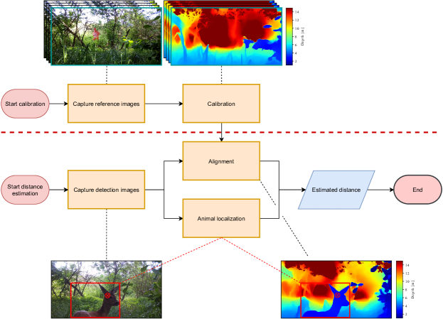
In this study, we propose a two-step pipeline to automate the estimation of camera-to-animal distances from monocular camera images. (1) The calibration workflow delivers the automated calibration of the observed transect using reference images and measurements. (2) The distance estimation workflow employs the calibration of the observed transect to automatically estimate camera-to-animal distances in camera trap images showing observed animals. Figure 1 depicts in the upper area the calibration workflow and in the lower area the distance estimation workflow.
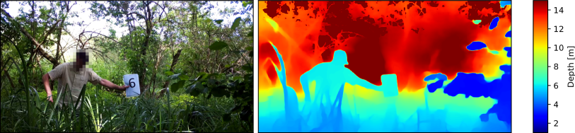
The calibration workflow starts with annotated reference images of the transect. The annotation of a reference image depicts the exact distance between the camera and a visible landmark (i.e., a distinct object placed on the transect with just the exact distance to the camera). Generally, several reference images are captured with landmarks placed at different distances, e.g., from 1 to 12 m. The calibration workflow generates from these given annotated reference images of a transect a calibrated depth image of the transect with exact distance measurements given in meters. These calibrated depth images are visualized as heatmaps where the distance is lowest in blue and highest in red. This calibration workflow is explained in more detail in section 3.1.
The distance estimation workflow starts with a so-called observation image, i.e., an image showing an animal observed in the transect. Using the calibrated depth image of the transect (delivered by the calibration workflow), an exact estimation of the camera-animal distance in meters is derived. This distance estimation workflow is explained in more detail in section 3.2.
2 Data material
The data for this study was collected in the conservation area ‘Hintenteiche bei Biesenbrow’ located in the Biosphere Reserve Schorfheide-Chorin. The data material is comprised of videos from 29 transects, captured using Bushnell Trophy CAM HD Agressor 119876 camera traps. The videos contain either greyscale infrared frames (captured at nighttime) or RGB (red, green, blue) color frames at 30 frames per second and a resolution of . We refer to greyscale and RGB images as intensity images. For each transect, a sequence of reference intensity images , with were sampled manually from designated reference videos. Every such image shows a landmark with a known distance to the camera, in distances of 1 meter, 2 meters, …, meters. These landmarks are established by a person showing a paper sheet depicting the distance to the camera by the number of meters. Figure 2 depicts two reference images with the researcher and the paper sheet positioned at a distance of 3 meters and 15 meters with respect to the camera, respectively. From the videos depicting observed animals, we automatically sample a single image every two seconds, from which both the manual as well as the automated distance measurements are derived. We refer to those images as observation images. To ensure no negative impact on further processing, we further remove metadata embedded visually inside each reference and observation image by cropping the bottommost , reducing the effective resolution to . We exclude five out of the 29 total transects (T03, T04, T07, T11, T12) which were set up in a suboptimal way (c.f. section 4.1), which led to poor results. Hence, we do not include these transects in our evaluation.
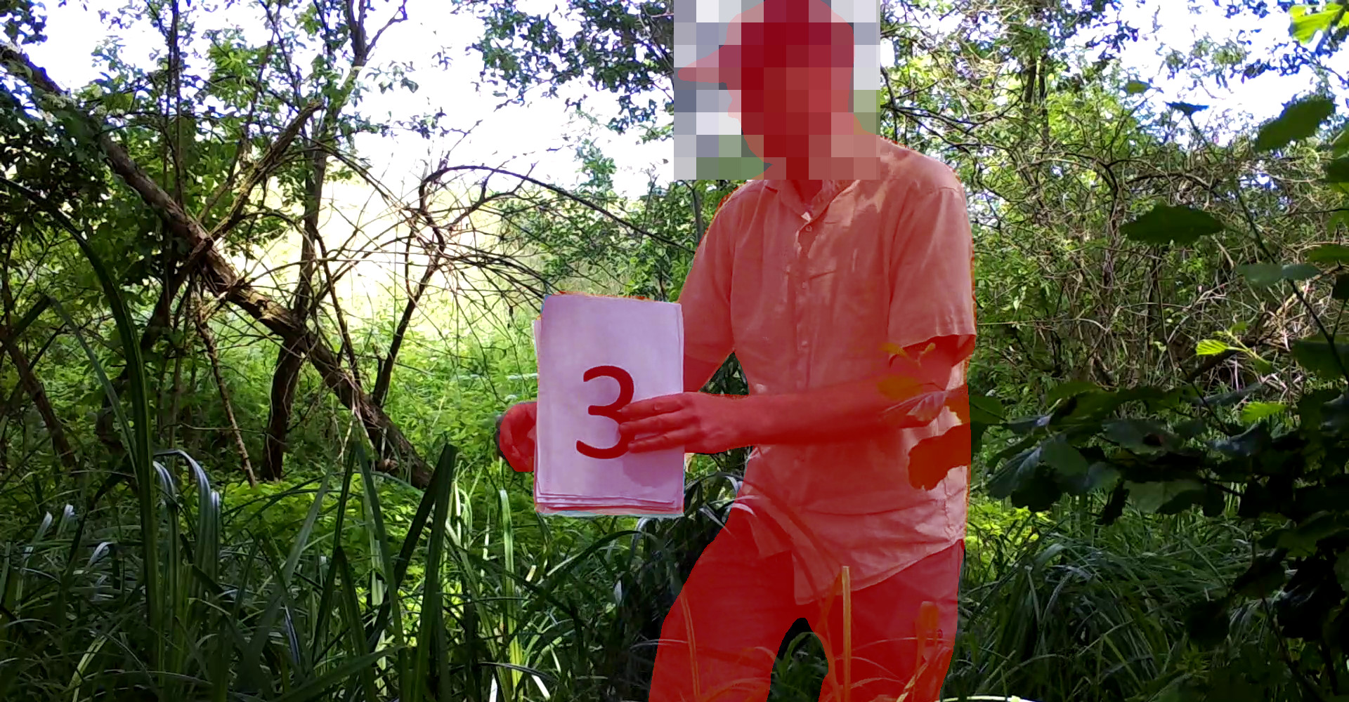
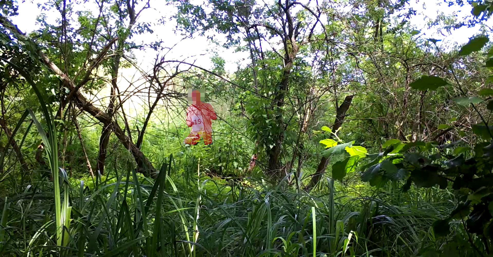
Table 1 shows the distribution of reference and observation images with respect to the transects.
| Transect | T01 | T02 | T05 | T06 | T08 | T09 | T10 | T13 | T14 | T15 | T16 | T17 |
|---|---|---|---|---|---|---|---|---|---|---|---|---|
| # Ref. Images | 7 | 7 | 11 | 14 | 12 | 13 | 4 | 9 | 10 | 10 | 5 | 5 |
| # Obs. Images | 4589 | 5753 | 920 | 925 | 942 | 1220 | 3246 | 1949 | 769 | 886 | 140 | 59 |
| Transect | T18 | T19 | T20 | T21 | T22 | T23 | T24 | T25 | T26 | T27 | T28 | T30 |
| # Ref. Images | 12 | 15 | 6 | 6 | 7 | 10 | 10 | 15 | 10 | 7 | 13 | 13 |
| # Obs. Images | 160 | 1111 | 549 | 5135 | 425 | 1210 | 299 | 422 | 332 | 125 | 8356 | 279 |
3 Methods
The challenge to overcome the distance estimation bottleneck in abundance estimation of unmarked animal populations with simple monocular cameras, is the derivation of precise distance estimations to objects in the observed scene from just one single image.
Recent developments have shown that detailed distance estimations can be derived from a single image in an end-to-end manner based on deep learning approaches (Facil et al., 2019). Meanwhile, various deep learning have shown their effectiveness to address the monocular depth estimation (MDE). In this study, we decide for the DPT (Dense Prediction Transformers) approach that has shown superior quantitative and qualitative results in MDE. This is achieved by training on millions of pairs of monocular camera images and the corresponding distance estimations for each pixel (Ranftl et al., 2020, 2021). The strength of DPT stems from employing a wide variety of training data from multiple sources.
3.1 Camera trap calibration
Calibration of a camera trap employs reference images that depict landmarks of known distances to the camera. It is important to note that the reference images may be acquired in a multitude of ways since our calibration method is agnostic to the exact generation of the reference images. In this study, the landmarks are established by a person showing a paper sheet depicting the distance to the camera by the number of meters (cf. fig. 2).
3.1.1 Uncalibrated depth images via monocular depth estimation
For each camera trap, there are reference images with a corresponding binary mask covering the landmark (depicted red in fig. 2) and the corresponding true distance between camera and landmark for . We refer to the -th reference image as the target reference image. The reference images are first propagated through the DPT (Ranftl et al., 2021) depth estimation model which results in uncalibrated disparity images depicting the pixel-wise inverse distances to scene objects in a relative way, i.e., depth image pixels in blue are closer than those in green that in turn are closer than those in yellow which in turn are closer than those in red. More precisely: the uncalibrated disparity images show inverse distance estimations up to an unknown scale parameter and an unknown shift parameter .
3.1.2 Calibrated depth images via RANSAC
Therefore, at least two landmarks with known distances to the camera must be used to determine both parameters. In this dataset, each of the reference images depicts exactly one landmark, i.e, the researcher with a paper sheet. Since the landmarks are distributed over all reference images , prior to the metric calibration, we align all uncalibrated disparity images to one common, yet not calibrated, scale. To be precise, for each uncalibrated disparity image with , we estimate two parameters , using the RANSAC approach (Fischler and Bolles, 1981), such that
| (1) |
where depicts all pixels in the disparity image outside the binary mask covering the landmark, i. e., all pixels depicting the visible stationary components of the observed scene. This alignment ensures the optimal alignment of all landmarks used in the next calibration step. Given the landmarks in the aligned uncalibrated disparity images with , the RANSAC approach (Fischler and Bolles, 1981) is then used to estimate the unknown scale parameter and the unknown shift parameter with the objective of minimizing the absolute disparity error:
| (2) |
where depicts all pixels in the disparity image within the binary mask covering the landmark. From these disparity values the median value is chosen for minimization due to the improved robustness when facing imperfect landmark masks compared to the mean. The real metric distance to the respective landmark (i.e., the ground truth) is depicted with , the shift and scale parameters of disparity image are given as and . The resulting calibrated disparity images and metric depth images are then given by equations 3 and 4, respectively:
| (3) |
| (4) |
Instead of metric distances with image values in we can deal with disparity values in where is the image width. This results in improved numerical stability and induces lower weighting of more distant landmarks, reflecting the lower accuracy of the depth estimation at large distances. We refer to and as the target reference disparity and depth images, respectively. This target reference depth image is highlighted in blue in figure 3.
3.2 Animal distance estimation
For each detected animal observation, we have to estimate a single metric distance to the animal. This objective demands to solve two requirements: (1) deriving a calibrated depth image of the camera trap image depicting the observed animal, (2) localization of the observed animal in this calibrated depth image .
3.2.1 Deriving a calibrated depth image for each animal observation
Sampling accurate distance information for each observation image employs the scale information of the calibration step described in section 3.1. We achieve this by transferring the scale of the calibrated reference disparity images to the estimated disparity images of each animal observation. One might think that a simpler approach would be to just sample the depth of the calibrated reference images. However, the scenes observed by the camera traps are highly dynamic (due to trees falling over, plants gaining or loosing leaves, etc.), leading to higher estimation errors when employing this strategy. Therefore, we employ again the monocular depth estimation by DPT Ranftl et al. (2021) to estimate first an uncalibrated disparity image of each observation image . We then transfer the metric scale acquired during calibration onto the uncalibrated disparity of each observation . From all possible calibrated reference disparity images to inform this metric scale we use the calibrated target reference disparity , i.e., the one representing the calibration landmark with the largest distance. This choice shows the minimum number of pixels depicting the calibration landmark and therefore the maximum number of image pixels with an associated depth value that depict the scene where the animal is observed. We transfer the scale of the target depth image to the uncalibrated observation disparity image by again estimating the scale and shift parameters and using RANSAC (Fischler and Bolles, 1981) while minimizing the absolute disparity error over the entire images, while excluding the calibration landmark and bounding boxes of detected animals (c.f. section 3.2.2):
| (5) |
3.2.2 Localization of the observed animal in this calibrated depth image
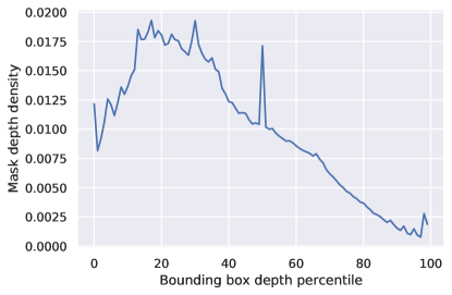
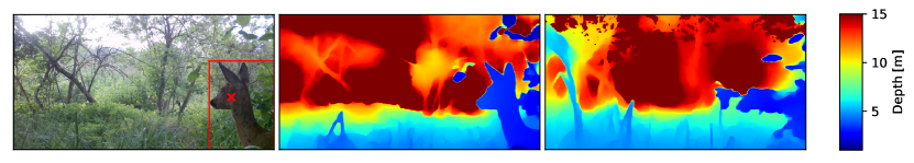
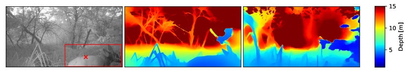
For animal detection we employ MegaDetector (Beery et al., 2019), a deep-learning animal detection model based on the Faster R-CNN (Ren et al., 2015) and Inception Resnet (Szegedy et al., 2017) architecture. It is trained using large amounts of images annotated by humans with bounding boxes for the object classes animal, human, and vehicle. We use this trained MegaDetector model and apply it to the observation image , resulting in a bounding box for each animal observed in . From all detected bounding boxes corresponding to a single observation, we infer a binary mask which is set to one at each pixel inside any detected bounding box and to zero everywhere else. This binary mask is used in equation 5. Then, we sample for each bounding the 20th percentile of the corresponding calibrated depth observation image . Figure 6 shows two exemplary observation images with corresponding detected bounding boxes, depth images and the locations of the sampled depth. This procedure is simple but effective. It is also intuitive, as the animals are mostly positioned on a much more distant background and slightly occluded by plants or trees. The 20th percentile of the depth then presents an accurate estimate of the true distance, as illustrated by figure 5. We also evaluated more sophisticated methods for precise localization such as class attention maps (CAMs, Zhou et al. (2016)) of species classification models (Microsoft Corporation, 2019) but found these models to fail in many instances when the animals are strongly occluded. The classification of animals is therefore performed by a human observer and not automated.
3.2.3 Metrics for evaluating measurement error
For evaluation, we employ the mean absolute distance estimation error over all observations , defined as:
| (6) |
and the mean distance estimation error in our evaluation, defined as:
| (7) |
where and represent the estimated and ground-truth distance of each observation, respectively.
3.3 Distance Estimation Workbench
We implement the above methodology using the Python programming language. The execution of the MegaDetector and DPT models is handled by the TensorFlow (Abadi et al., 2015) and PyTorch (Paszke et al., 2019) libraries, respectively. The RANSAC (Fischler and Bolles, 1981) implementation is provided by Scikit-learn (Pedregosa et al., 2011). To make our methodology available to other researchers, we provide it in the form of a simple graphical user interface, which we call Distance Estimation Workbench. The Distance Estimation Workbench allows starting and stopping individual parts of the calibration and distance estimation workflows. Input and output is follows a standardized directory structure for image data and CSV spreadsheet files are used for metadata and ground truth measurements. This allows efficient processing of large datasets without manual interaction. The executable Distance Estimation Workbench is available, together with accompanying documentation and a minimal example dataset, at: https://timm.haucke.xyz/publications/distance-estimation-animal-abundance
4 Evaluation and discussion
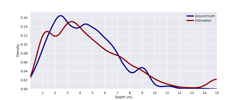
For the resulting distance estimations to be usable for the various methods available for the estimation of abundance of unmarked animal populations, it is important that our estimation method produces a distance distribution as close to the ground truth and as unbiased as possible. As can be seen in figure 7, the distribution of estimated distances indeed reflects the ground truth distribution. At both distributions differ by about 4 percentage points while the difference at is about 1 percentage point.
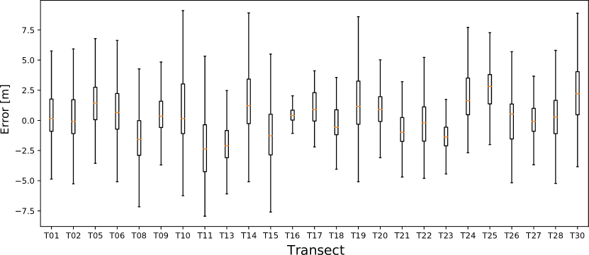
We achieve a mean distance error of and a mean absolute distance error of . The small positive bias of our method can be explained by the distribution of distance values in the calibrated depth images. Large parts of the depth images show background areas with arbitrarily large distances. If an animal is falsely detected in such an area, a very large distance is falsely estimated. Both the mean and the mean absolute distance error measures depend strongly on the transect, as can be seen in figure 8. High estimation errors can be observed with dense vegetation directly in front of the camera (e.g., T24), as the employed monocular depth estimation tends to smooth out the estimated disparity images, which is especially damaging for small cavities in the vegetation, in which the background then appears closer than it truly is. In this case, the initial calibration (c.f. section 3.1) fails because the known landmarks appear to be in a single plane. In other transects (e.g., T02), the forest ground is only visible to a small degree. This apparently also reduces monocular depth estimation accuracy because important context information about the relative location of objects in the scene is lost.
4.1 Camera trap setup guidelines
The choice of scene and the camera setup is therefore an important factor for the success of our method. A calibration result of a well-conditioned setup can be seen in figure 9. We want to provide researchers with guidelines on where and how to best place camera traps in the future to make the best use of our method and therefore make the following recommendations:
-
1.
Camera traps should be tightly secured to stationary objects, i.e. trees. This reduces camera motion and hence ensures a strong overlap of observation images with reference images
-
2.
generally, camera trapping benefits from a free field of view, therefore it should be free of vegetation inside a radius of three meters
-
3.
at least the bottom third of the image produced by the camera trap should be covered by the ground to ensure enough context information for the monocular depth estimation
-
4.
if the situation allows, artificial (e.g. ranging rods) or natural (e.g. trees, rocks, logs) (Palencia et al., 2021) reference objects could be permanently placed in the scene and incorporated in our automated method. A minimum of two reference objects are required for our calibration workflow, however, the more reference objects are captured, the more robust the calibration becomes
4.2 Evaluating distance estimation effort
To quantify the reduction of the manual distance estimation workload facilitated by our method, we conducted a user study with five users experienced with wildlife monitoring using camera trap imagery. Out of the data described in table 1, we randomly chose five transects, out of which we randomly sampled five detection videos with no more than one single animal present at a time. The participants of the study are then asked to apply the manual distance estimation process (cf. appendix A). We chose only observations with at most a single animal present at a time to prevent ambiguous assignments between multiple individuals over the participants and to therefore be able to quantify the deviation of distance estimations between participants. The time needed by a participant to compare the position of an observed animal in a video frame to the different distances in the reference video clips and estimate the distance has been measured to lie between and . The mean time needed per observation is .
We then estimate the workload of manual distance estimation of the complete dataset by assuming that every observation image shows only a single animal. Our comparison is therefore based on the processing time per observation image. This results in person hours for the complete dataset of observation images. However, about of the total observation images contain more than one animal. Therefore, the person hours slightly underestimate the manual distance estimation workload for the complete dataset by assuming that every observation image shows only a single animal.
Our automated distance estimation pipeline requires person hours for annotating reference images and 24 hours for automated distance estimation for all observation images.
The ratio between the complete manual distance estimation effort () and the complete automated distance estimation effort ( + ) is . Since the time required for the manual distance estimation is underestimated, this ratio of is a lower bound of the speedup factor. The same holds for the speedup factor of the purely manual workload, which is .
We also compared the quality of the manual distance estimations produced by the participants. In 9% of cases, the participants disagree on whether an animal is visible in the image. The mean standard deviation between the participants over the remaining 91% of measurements is , suggesting a lower bound of the achievable accuracy.
5 Conclusion
Methods for abundance estimation of unmarked animal populations from camera traps all require an estimate of the effective area surveyed, which is usually done by deriving camera-to-animal observation distances. This is time-consuming, error-prone and subjective, which motivates our automated distance estimation method based on monocular depth estimation and a robust calibration workflow.
Our method imposes no constraints on specific camera hardware and is therefore applicable to a wide variety of datasets. In our experiments, we succeed in closely matching the true distance distribution.
Thereby we successfully overcome the distance estimation bottleneck in abundance estimation of unmarked animal populations. Our automated method achieves a mean distance error of only 0.14 m, it reduces the manual effort by a factor of and the total processing time by a factor of . This facilitates large-scale, automated abundance estimation of unmarked animal populations.
Future work could improve the temporal stability of monocular depth estimation and in turn further improve the distance estimation accuracy.
In cases where videos or image sequences are available for each animal observation, multi-object tracking approaches would likely reduce false positive and false negative observations by combining information from multiple frames.
Acknowledgments
This research has been funded in part by the Federal Ministry of Education and Research (www.bmbf.de) of the Federal Republic of Germany under grant number 01DK17048. We would like to thank the Helversen’sche Stiftung for providing permission and access to the FFH conservation area ‘Hintenteiche bei Biesenbrow’ and are grateful for support of our work by Dorothea Dietrich, Dietmar Nill, Ulrich Stöcker and Thomas Volpers. We thank Dr. Martin Flade and Rüdiger Michels from the Biosphere Reserve Schorfheide-Chorin. We thank the participants of the user study. We thank Frank Schindler for proofreading the manuscript.
Appendix A Manual distance estimation process
References
- Abadi et al. (2015) Abadi, M., Agarwal, A., Barham, P., Brevdo, E., Chen, Z., Citro, C., Corrado, G.S., Davis, A., Dean, J., Devin, M., Ghemawat, S., Goodfellow, I., Harp, A., Irving, G., Isard, M., Jia, Y., Jozefowicz, R., Kaiser, L., Kudlur, M., Levenberg, J., Mané, D., Monga, R., Moore, S., Murray, D., Olah, C., Schuster, M., Shlens, J., Steiner, B., Sutskever, I., Talwar, K., Tucker, P., Vanhoucke, V., Vasudevan, V., Viégas, F., Vinyals, O., Warden, P., Wattenberg, M., Wicke, M., Yu, Y., Zheng, X., 2015. TensorFlow: Large-scale machine learning on heterogeneous systems. URL: https://www.tensorflow.org/. software available from tensorflow.org.
- Beery et al. (2019) Beery, S., Morris, D., Yang, S., 2019. Efficient pipeline for camera trap image review. arXiv preprint arXiv:1907.06772 .
- Facil et al. (2019) Facil, J.M., Ummenhofer, B., Zhou, H., Montesano, L., Brox, T., Civera, J., 2019. Cam-convs: camera-aware multi-scale convolutions for single-view depth, in: Proceedings of the IEEE/CVF Conference on Computer Vision and Pattern Recognition, pp. 11826–11835.
- Fischler and Bolles (1981) Fischler, M.A., Bolles, R.C., 1981. Random sample consensus: a paradigm for model fitting with applications to image analysis and automated cartography. Communications of the ACM 24, 381–395.
- Gilbert et al. (2021) Gilbert, N.A., Clare, J.D., Stenglein, J.L., Zuckerberg, B., 2021. Abundance estimation of unmarked animals based on camera-trap data. Conservation Biology 35, 88–100.
- (6) Haglöf Sweden AB, . Vertex iv. https://web.archive.org/web/20210121013130/http://www.haglofcg.com/index.php/en/products/instruments/height/341-vertex-iv. Accessed: 2021-01-21.
- Haucke and Steinhage (2021) Haucke, T., Steinhage, V., 2021. Exploiting depth information for wildlife monitoring. arXiv:2102.05607.
- Henrich et al. (2021) Henrich, M., Heurig, M., Fiderer, C., 2021. Distance measurement in wildlife monitoring using ultrasonic distance sensors. Faculty of Environment and Natural Ressources, Univ. of Freiburg. Personal communication.
- Hofmeester et al. (2017) Hofmeester, T.R., Rowcliffe, J.M., Jansen, P.A., 2017. A simple method for estimating the effective detection distance of camera traps. Remote Sensing in Ecology and Conservation 3, 81–89.
-
Howe et al. (2017)
Howe, E.J., Buckland, S.T.,
Després-Einspenner, M.L., Kühl, H.S.,
2017.
Distance sampling with camera traps.
Methods in Ecology and Evolution
8, 1558–1565.
URL: https://besjournals.onlinelibrary.wiley.com/doi/abs/10.1111/2041-210X.12790,
doi:10.1111/2041-210X.12790,
arXiv:https://besjournals.onlinelibrary.wiley.com/doi/pdf/10.1111
/2041-210X.12790. - Marcus Rowcliffe et al. (2011) Marcus Rowcliffe, J., Carbone, C., Jansen, P.A., Kays, R., Kranstauber, B., 2011. Quantifying the sensitivity of camera traps: an adapted distance sampling approach. Methods in Ecology and Evolution 2, 464–476.
- Microsoft Corporation (2019) Microsoft Corporation, 2019. Ai for earth species classification. https://github.com/microsoft/SpeciesClassification. Accessed: 2021-02-18.
- Moeller et al. (2018) Moeller, A.K., Lukacs, P.M., Horne, J.S., 2018. Three novel methods to estimate abundance of unmarked animals using remote cameras. Ecosphere 9, e02331.
- Nakashima et al. (2018) Nakashima, Y., Fukasawa, K., Samejima, H., 2018. Estimating animal density without individual recognition using information derivable exclusively from camera traps. Journal of Applied Ecology 55, 735–744.
- O’Connell et al. (2011) O’Connell, A.F., Nichols, J.D., Karanth, K.U., 2011. Camera traps in animal ecology: methods and analyses. volume 271. Springer.
- Palencia et al. (2021) Palencia, P., Rowcliffe, J.M., Vicente, J., Acevedo, P., 2021. Assessing the camera trap methodologies used to estimate density of unmarked populations. Journal of Applied Ecology 58, 1583–1592.
- Paszke et al. (2019) Paszke, A., Gross, S., Massa, F., Lerer, A., Bradbury, J., Chanan, G., Killeen, T., Lin, Z., Gimelshein, N., Antiga, L., Desmaison, A., Kopf, A., Yang, E., DeVito, Z., Raison, M., Tejani, A., Chilamkurthy, S., Steiner, B., Fang, L., Bai, J., Chintala, S., 2019. Pytorch: An imperative style, high-performance deep learning library, in: Wallach, H., Larochelle, H., Beygelzimer, A., d'Alché-Buc, F., Fox, E., Garnett, R. (Eds.), Advances in Neural Information Processing Systems 32. Curran Associates, Inc., pp. 8024–8035. URL: http://papers.neurips.cc/paper/9015-pytorch-an-imperative-style-high-performance-deep-learning-library.pdf.
- Pedregosa et al. (2011) Pedregosa, F., Varoquaux, G., Gramfort, A., Michel, V., Thirion, B., Grisel, O., Blondel, M., Prettenhofer, P., Weiss, R., Dubourg, V., Vanderplas, J., Passos, A., Cournapeau, D., Brucher, M., Perrot, M., Duchesnay, E., 2011. Scikit-learn: Machine learning in Python. Journal of Machine Learning Research 12, 2825–2830.
- Ranftl et al. (2021) Ranftl, R., Bochkovskiy, A., Koltun, V., 2021. Vision transformers for dense prediction. arXiv preprint arXiv:2103.13413 .
- Ranftl et al. (2020) Ranftl, R., Lasinger, K., Hafner, D., Schindler, K., Koltun, V., 2020. Towards robust monocular depth estimation: Mixing datasets for zero-shot cross-dataset transfer. IEEE Transactions on Pattern Analysis and Machine Intelligence (TPAMI) .
- Ren et al. (2015) Ren, S., He, K., Girshick, R., Sun, J., 2015. Faster r-cnn: Towards real-time object detection with region proposal networks. Advances in neural information processing systems 28, 91–99.
- Rowcliffe et al. (2008) Rowcliffe, J.M., Field, J., Turvey, S.T., Carbone, C., 2008. Estimating animal density using camera traps without the need for individual recognition. Journal of Applied Ecology 45, 1228–1236.
- Steenweg et al. (2017) Steenweg, R., Hebblewhite, M., Kays, R., Ahumada, J., Fisher, J.T., Burton, C., Townsend, S.E., Carbone, C., Rowcliffe, J.M., Whittington, J., et al., 2017. Scaling-up camera traps: Monitoring the planet’s biodiversity with networks of remote sensors. Frontiers in Ecology and the Environment 15, 26–34.
- Szegedy et al. (2017) Szegedy, C., Ioffe, S., Vanhoucke, V., Alemi, A.A., 2017. Inception-v4, inception-resnet and the impact of residual connections on learning, in: Proceedings of the Thirty-First AAAI Conference on Artificial Intelligence, AAAI Press. p. 4278–4284.
- Zhou et al. (2016) Zhou, B., Khosla, A., Lapedriza, A., Oliva, A., Torralba, A., 2016. Learning deep features for discriminative localization, in: Proceedings of the IEEE conference on computer vision and pattern recognition, pp. 2921–2929.