Exploiting Elasticity in Tensor Ranks for Compressing Neural Networks

Abstract

Elasticities in depth, width, kernel size and resolution have been explored in compressing deep neural networks (DNNs). Recognizing that the kernels in a convolutional neural network (CNN) are 4-way tensors, we further exploit a new elasticity dimension along the input-output channels. Specifically, a novel nuclear-norm rank minimization factorization (NRMF) approach is proposed to dynamically and globally search for the reduced tensor ranks during training. Correlation between tensor ranks across multiple layers is revealed, and a graceful tradeoff between model size and accuracy is obtained. Experiments then show the superiority of NRMF over the previous non-elastic variational Bayesian matrix factorization (VBMF) scheme.

I Introduction

Deep learning and deep neural networks (DNNs) have achieved breakthroughs in various artificial intelligence (AI) applications, including classification [1], object detection [2], and semantic segmentation [3]. However, DNN structures are getting deeper and larger, making it challenging to deploy DNNs on edge devices with limited resources. This dilemma has motivated the search for compact neural networks with lower computation and memory cost. Various neural network compression techniques have been proposed, which can be mainly divided into three categories, namely, pruning [4], quantization [5, 6], and low-rank approximation [7].

Tensor factorization [8] belongs to the third category and is a powerful tool to compress convolutional neural networks (CNNs). It offers efficient low-rank approximations of the convolution kernels that can be regarded as a 4-way tensor, resulting in a significant reduction of parameters at the expense of only a small drop in output accuracy. Canonical polyadic (CP) decomposition is a widely used tensor decomposition method, which has been applied to decompose a 4-way kernel tensor into four sequential smaller convolutional (CONV) layers [9]. However, this approach is highly sensitive to the decomposition and only works well when one or two layers are compressed. Besides, the CP ranks need to be selected manually which is time-consuming without any optimality guarantee. To address this, Tucker-2 decomposition has been proposed to factorize a CONV layer into three smaller ones with Tucker ranks set by variational Bayesian matrix factorization (VBMF) [10]. Although VBMF provides a principled way to prescribe ranks, it suffers from two major drawbacks: 1) it does not guarantee a globally or locally optimal combination of ranks; 2) once the ranks are set, they remain fixed during the fine-tuning stage, making it impossible to seek better ranks dynamically.

To improve upon VBMF rank selection, an intuitive way is to traverse all rank combinations. This is similar to the neural architecture search (NAS) [11], but obviously such brute-force method is time-consuming and computationally prohibitive. Recently, the once-for-all (OFA) approach has been proposed using a progressive shrinking algorithm to effectively train a network that supports diverse architectural settings with elastic depth, width, kernel size and resolution [12]. Along a related but orthogonal direction, we devise a new way to exploit elasticity in tensor ranks for compressing CNNs. Our baseline is the work in [10] that compresses the input-output channel dimensions using Tucker-2 decomposition (the spatial dimensions, typically $3\times 3$ or $5\times 5$, are too small to be compressed). However, instead of fixing the ranks and prescribing the CNN structure before fine-tuning, our scheme dynamically finds the required Tucker-2 ranks via a nuclear-norm-like regularizer added to the normal loss function.

To our best knowledge, this is the first time that Tucker ranks of kernel tensors are found on-the-fly during training. We further show that the ranks located by our nuclear-norm rank minimization factorization (NRMF) consistently achieve higher compression ratios than VBMF ranks with only a slight accuracy drop. Our key contributions are:

• We exploit the elasticity in tensor ranks during training by adding a nuclear-norm-like regularizer to the loss function, in contrast to everything being hardwired at the beginning as in the VBMF approach.

• By analyzing variation of ranks in early CONV layers to deeper ones, one observes an interesting decreasing of ranks in the last several layers. This could be guidance to remove redundancy in wide layers without much information loss.

• The proposed NRMF is a generic, dynamic rank selection method which can be applied for low-rank CNN approximation together with other techniques such as quantization and pruning.

Experimental results on some popular networks demonstrate that the ranks obtained by our proposed method are better choices than VBMF-based Tucker-2 decomposition, which achieve higher compression ratios and maintain good performance. In the following, Section II shows some related works. Section III introduces necessary tensor basics. Details of the proposed method are described in Section IV. Experiments are given in Section V and Section VI draws the conclusion.

II Related Work

Tensor Decomposition. In CNNs, computational cost during inference is dominated by the evaluation of convolutional layers. With the goal of speeding up inference, many CNN compression tools based on tensor decomposition have been proposed. Tensor-train (TT) decomposition has been applied to fully-connected layers [13] and CONV layers [14]. CP [15] and Tucker [10] decomposition are also used to model compression. However, the CP approach requires manual rank setting, and is highly sensitive and only works for one or two layers. Consequently, we use the Tucker-2 decomposition in [10] as our baseline for compressing CONV layers.

Rank Selection. Ranks are key parameters in tensor decomposition for trading compression with model accuracy. In order to find the optimal ranks for different layers, several rank selection methods have been proposed. Reconstruction optimization [8] uses CP decomposition. Ref [16] has proposed a heuristic fitness-based rank selection method. However, these methods have limitations in multi-rank selection and suffer from convergence problems during optimization. A sensitivity-driven rank selection considering the ratio threshold of singular values (SVs) is introduced in [17], but the wide range of the criterion renders the decision difficult. Variational Bayesian matrix factorization (VBMF) [18] is a tool to select ranks for Tucker-2 decomposition by unfolding a tensor along different modes. VBMF offers a probabilistic ground to automatically find the ranks and noise variance, and is employed in [10] to determine ranks. However, the matrix-wise independence in VBMF factors is hard to justify. Also, it is difficult to use VBMF to fit a given compression ratio since the parameters of controlling ranks are so sensitive that minor modifications might lead to zero ranks.

Pruning. The popular and effective DNN compression pipeline involves training, pruning and re-training [4], which takes parameter magnitude for thresholding. There are various extensions: pruning cost measurement  [19], soft weight-sharing and factorized Dirac posteriors [20], dynamic sparse training [21] etc. Instead of pruning weights in neural networks, [12] proposes progressive shrinking to reduce multiple dimensions (viz. depth, width, kernel size and resolution) of the whole network. Besides, it targets searching the best sub-networks which maintain accuracy rather than pruning just one network. As a generalization of pruning methods, ranks used in compressing layers via Tucker decomposition can also be considered as an elastic dimension. While it has high computational cost with Tucker decomposition for every rank combination, we propose to not actually factorize during training, but use a data-driven optimization to strike a balance between accuracy and compression.

III Preliminary

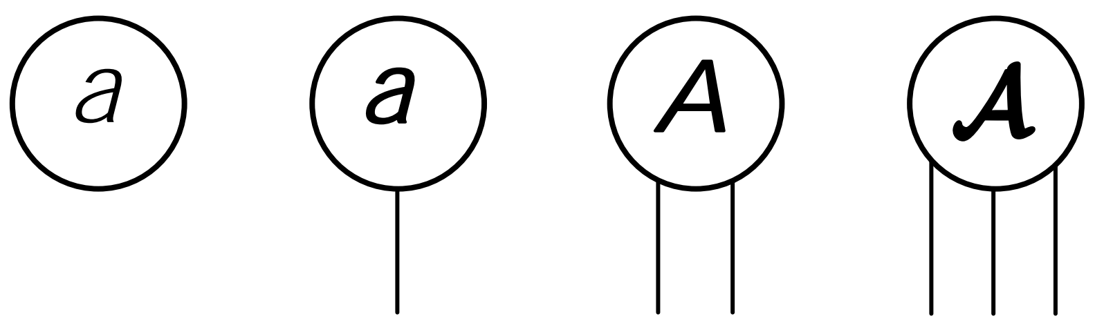
Figure 1: Graphical representation of a scalar $a$, vector $\mathbf{a}$, matrix $\mathbf{A}$, and third-order tensor $\bm{\mathcal{A}}$.

Tensors are high-dimensional generalization of vectors and matrices [22]. In the following, we use Roman letters $a,b,\ldots$ to denote scalars; boldface letters $\mathbf{a,b},\ldots$ to denote vectors; boldface capital letters $\mathbf{A,B},\ldots$ to denote matrices; and boldface capital calligraphic letters $\bm{\mathcal{A}},\bm{\mathcal{B}},\ldots$ to denote tensors. Tensor network diagram is a handy way of representing tensors as shown in Figure 1, wherein each node denotes a tensor whose order is represented by the number of free edges. Reshaping is a basic tensor operation, by adopting a MATLAB-like notation, “reshape($\bm{\mathcal{A}},[m_{1},m_{2},\ldots,m_{p}]$)”, we reshape a $d$-way tensor $\bm{\mathcal{A}}\in\mathbb{R}^{I_{1}\times I_{2}\times\ldots\times I_{d}}$ into another $p$-way tensor with dimensions $m_{1},m_{2},\ldots,m_{p}$. The total number of elements of $\bm{\mathcal{A}}$ is $\prod_{k=1}^{d}I_{k}$, which must be equal to $\prod_{k=1}^{p}m_{k}$. Tensor-matrix multiplication is a generalization of the matrix-matrix product to the multiplication of a matrix with a $d$-way tensor along one of its $d$ modes.

Definition 1

($k$-mode product) The $k$-mode product of tensor $\bm{\mathcal{G}}\in\mathbb{R}^{R_{1}\times\cdots\times R_{d}}$ with a matrix $\bm{U}\in\mathbb{R}^{J\times R_{k}}$ is denoted $\bm{\mathcal{A}}=\bm{\mathcal{G}}\times_{k}\bm{U}$ and defined by

$$\small\bm{\mathcal{A}}(r_{1},\cdots,r_{k-1},j,r_{k+1},\cdots,r_{d}) =\hfill$$

$$\small\sum_{r_{k}=1}^{R_{k}}\bm{U}(j,r_{k})\bm{\mathcal{G}}(r_{1},\cdots,r_{k-1},r_{k}, r_{k+1},\cdots,r_{d})$$

where $\bm{\mathcal{A}}\in\mathbb{R}^{R_{1}\cdots R_{k-1}\times J\times R_{k+1}\cdots\times R_{d}}$.

Definition 2

(Full multilinear product) The full multilinear product of a tensor $\bm{\mathcal{G}}\in\mathbb{R}^{R_{1}\times\cdots\times R_{d}}$ with matrices $\bm{U}^{(1)},\bm{U}^{(2)},\ldots,\bm{U}^{(d)}$, where $\bm{U}^{(k)}\in\mathbb{R}^{I_{k}\times R_{k}}$, is defined by $\bm{\mathcal{A}}=\bm{\mathcal{G}}\times_{1}\bm{U}^{(1)}\times_{2}\bm{U}^{(2)}\ldots\times_{d}\bm{U}^{(d)}$, where $\bm{\mathcal{A}}\in\mathbb{R}^{I_{1}\times\ldots\times I_{d}}$.

Definition 3

(Tucker decomposition) Tucker decomposition represents a $d$-way tensor $\bm{\mathcal{A}}\in\mathbb{R}^{I_{1}\times\ldots\times I_{d}}$ as the full multilinear product of a core tensor $\bm{\mathcal{G}}\in\mathbb{R}^{R_{1}\times R_{2}\times\ldots\times R_{d}}$ and a set of factor matrices $\bm{U}^{(k)}\in\mathbb{R}^{I_{k}\times R_{k}}$, for $k=1,2,\ldots,d$. Writing out $\bm{U}^{(k)}=[\bm{u}_{1}^{(k)},\bm{u}_{2}^{(k)},\ldots,\bm{u}_{R_{k}}^{(k)}]$ for $k=1,2,\ldots,d$,

$$\small\bm{\mathcal{A}} =\small\sum\limits^{R_{1}}_{r_{1}=1}\cdots\sum\limits^{R_{d}}_{r_{d}=1}\bm{\mathcal{G}}(r_{1},\ldots,r_{d})(\bm{u}_{r_{1}}^{(1)}\circ\cdots\circ\bm{u}_{r_{d}}^{(d)})$$

$$=\small\bm{\mathcal{G}}\,{\times_{1}}\,\bm{U}^{(1)}\,{\times_{2}}\,\bm{U}^{(2)}\cdots{\times_{d}}\,\bm{U}^{(d)}$$

where $r_{1},r_{2},\ldots,r_{d}$ are auxiliary indices that are summed over, and $\circ$ denotes the outer product. The dimensions $(R_{1},R_{2},\ldots,R_{d})$ are called the Tucker ranks.

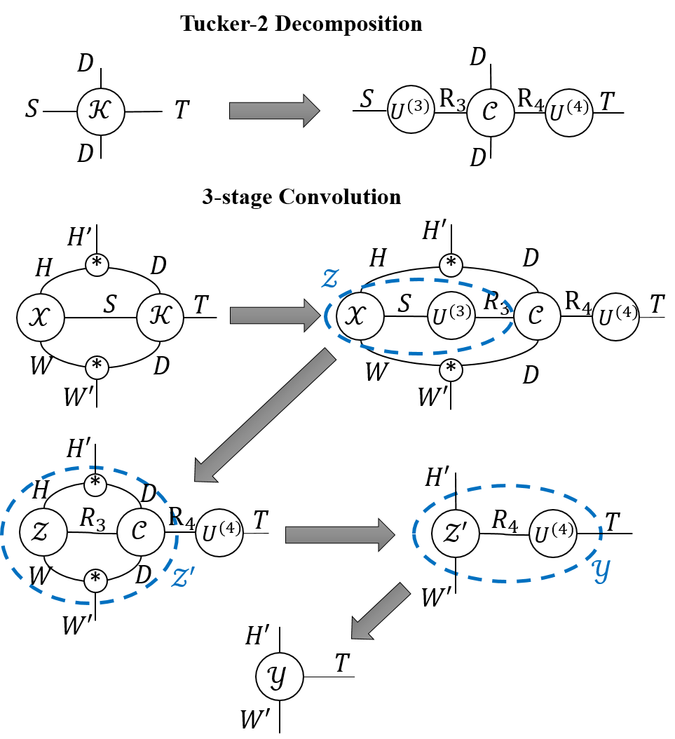
Figure 2: (Upper) Tucker-2 decomposition of a kernel tensor $\bm{\mathcal{K}}$. (Lower) Convolution process on the decomposed kernel tensor where $\bm{\mathcal{X}}$ is the input feature and $\bm{U^{(3)}},\bm{\mathcal{C}},\bm{U^{(4)}}$ are three sequential smaller CONV layers after factorization with kernel size $1\times 1$, $D\times D$ and $1\times 1$, respectively.

With the definition of Tucker decomposition in place, the Tucker-2 decomposition [10] is easily understood. A CONV layer can be regarded as a $4$-way kernel tensor of size [height $\times$ width $\times$ #input $\times$ #outputs], and the Tucker decomposition is applied only to the last two modes instead of all four since spatial dimensions are too small (e.g., $3\times 3$ or $5\times 5$) to be decomposed. Figure 2 shows the graphical representation of Tucker-2 decomposition on a kernel tensor $\bm{\mathcal{K}}$ in the upper part, and the convolution process after the decomposition in the lower part. The Tucker ranks play a crucial role in approximating the original full tensor, which determines the performance of the compressed CNNs.

VBMF is employed in [10] to find Tucker ranks, which we briefly describe here. The upper part of Figure 3 shows mode-$3$ and mode-$4$ matricizations of the $4$-way kernel tensor $\bm{\mathcal{W}}\in\mathbb{R}^{D\times D\times S\times T}$. When searching rank $R_{3}$ for $\bm{W}^{(1)}\in\mathbb{R}^{S\times(T\times D\times D)}$, VBMF treats $\bm{W}^{(1)}$ as the observation matrix, which is the sum of a target matrix $\bm{U}\in\mathbb{R}^{S\times(T\times D\times D)}$ and a noise matrix $\bm{E}\in\mathbb{R}^{S\times(T\times D\times D)}$ such that $\bm{W}^{(1)}=\bm{U}+\bm{E}$. The goal of VBMF is to find a low-rank $\bm{U}$ by filtering out the noise on $\bm{W}^{(1)}$. Being a probabilistic matrix factorization tool [18], VBMF finds the noise variance on $\bm{W}^{(1)}$ automatically, then gets the rank $R_{3}$ of $\bm{U}$, and similarly for $R_{4}$.

Figure 3: (Upper) Mode-3 and mode-4 matricizations of $4$-way kernel tensor $\bm{\mathcal{W}}_{m}$. (Lower) NRMF rank selection strategy.

IV The Proposed NRMF Scheme

Here we propose a novel way to exploit elasticity in Tucker ranks. First, we introduce a nuclear-norm-based regularizer, and demonstrate how it can dynamically locate the ranks during training. Algorithm 1 captures the workflow.

IV-A Regularizer

Given a CNN with $M$ convolution filter tensors $\bm{\mathcal{W}}_{m}\in\mathbb{R}^{D_{m}\times D_{m}\times S_{m}\times T_{m}}$, $m=1,2,\cdots,M$, where $D_{m}\times D_{m}$ denotes the kernel size, $S_{m}$ and $T_{m}$ are input and ouput channels for $m$th convolution layer, respectively. Then, we get $\bm{W}_{m}^{(1)}\in\mathbb{R}^{S_{m}\times(T_{m}\times D_{m}\times D_{m})}$ and $\bm{W}_{m}^{(2)}\in\mathbb{R}^{T_{m}\times(S_{m}\times D_{m}\times D_{m})}$ as mode-3 and mode-4 matricizations of $\bm{\mathcal{W}}_{m}$. Next, a regularization term $L_{n}$ is added to the training loss that penalizes increase in the sum of singular values (SVs) of matrices $\bm{W}_{m}^{(1)}\bm{W}_{m}^{(1)T}$ and $\bm{W}_{m}^{(2)}\bm{W}_{m}^{(2)T}$:

$$L_{n}=\frac{1}{2M}\sum_{m=1}^{M}(tr(\bm{W}_{m}^{(1)}\bm{W}_{m}^{(1)T})+tr(\bm{W}_{m}^{(2)}\bm{W}_{m}^{(2)T})).$$ (1)

Because $tr(\bm{W}_{m}^{(1)}\bm{W}_{m}^{(1)T})$ and $tr(\bm{W}_{m}^{(2)}\bm{W}_{m}^{(2)T})$ are also nuclear norms of $\bm{W}_{m}^{(1)}\bm{W}_{m}^{(1)T}$ and $\bm{W}_{m}^{(2)}\bm{W}_{m}^{(2)T}$, respectively, we call this trace loss a nuclear-norm loss.

IV-B Modified Loss Function

Having the regularizer, we can train a CNN directly through back-propagation algorithm to obtain both truncated ranks and a new way of initialization which preserves compressed information from the original CNN. Given the training dataset $D=\{(\bm{x}_{1},\bm{y}_{1}),(\bm{x}_{2},\bm{y}_{2}),\cdots,(\bm{x}_{N},\bm{y}_{N})\}$ and weights parameter $\bm{\mathcal{W}}$ in the network, our initialization is determined by:

$$\mathcal{J}(\bm{\mathcal{W}}) =\frac{1}{N}(\sum_{i=1}^{N}\mathcal{L}((\bm{x}_{i},\bm{y}_{i}),\bm{\mathcal{W}}))+\alpha L_{n}(\bm{\mathcal{W}}_{cl}),$$ (2)

$$\bm{w}^{*} =\arg\min_{\bm{\mathcal{W}}}\mathcal{J}(\bm{\mathcal{W}}),$$ (3)

where $\mathcal{L}$ is the loss function, e.g., cross-entropy loss in classification, $\bm{\mathcal{W}}_{cl}\subseteq\bm{\mathcal{W}}$ are filter weights for all convolution layers with kernel size larger than $1\times 1$, $\alpha$ is the scaling factor for the rank regularization term.

The regularizer $L_{n}$ tends to suppress non-zero SVs and yields smaller ranks. However, stronger suppression of SVs incurs increase in the loss function, which counteracts the compression level. Consequently, it becomes a game between the estimation loss term and the regularization term, through which our method can dynamically find elastic ranks that strike a balance between performance and Tucker-2 ranks.

IV-C Rank Selection

The proposed regularizer facilitates the learning of ranks to achieve high compression ratios without much accuracy loss. After training, the SVs in $\bm{W}_{m}^{(1)}\bm{W}_{m}^{(1)T}$ and $\bm{W}_{m}^{(2)}\bm{W}_{m}^{(2)T}$ are suppressed to have nearly zero tails. By considering sum of these SVs as “energy” in the original weight tensor, we use a threshold ratio $p$ to retain the leading singular vectors and the number of SVs which preserve a certain percentage of energy, as detailed in Algorithm 1. Because we are minimizing the sum of SVs while keeping a balance between estimation accuracy and compression ratio using threshold $p$, initialization for fine-tuning after doing Tucker-2 decomposition preserves most energy in the original network without much information loss. However, the accuracy still drops after Tucker-2 truncation, which can be recovered by fine-tuning with our Tucker-based initialization.

Algorithm 1 Nuclear-norm rank minimizing factorization (NRMF)-based training for dynamic Tucker-2 rank finding.

0:  A CNN with kernel tensors $\{\bm{\mathcal{W}}_{m}\in\bm{\mathcal{W}}|\bm{\mathcal{W}}_{m}\in\mathbb{R}^{D_{m}\times D_{m}\times S_{m}\times T_{m}}$, $m=1,2,\ldots,M\}$, threshold $p$, scaling coefficient $\alpha$, optimizer $\mathcal{L}$, learning rate $lr$, dataset $D$, number of training epochs $N$.

0:  Tucker ranks $R_{m}^{(3)},R_{m}^{(4)}$ with $m=1,2,\ldots,M$.

  NRMF-based optimizer $\mathcal{J}$ in form of Eqn.(2) $\leftarrow\mathcal{L},\alpha,\bm{\mathcal{W}}$

  for $i=1,2,\ldots,N$ do

     $\bm{\mathcal{W}}\leftarrow\bm{\mathcal{W}}+lr*\frac{\partial\mathcal{J}(D,\bm{\mathcal{W}})}{\partial\bm{\mathcal{W}}}$

  end for

  for $m=1,2,\cdots,M$ do

     $\bm{W}_{m}^{(1)}\leftarrow$ reshape $(\bm{\mathcal{W}}_{m},[S_{m},(T_{m}\times D_{m}\times D_{m})])$

     $\bm{W}_{m}^{(2)}\leftarrow$ reshape $(\bm{\mathcal{W}}_{m},[T_{m},(S_{m}\times D_{m}\times D_{m})])$

     $\lambda_{m}^{(i_{m})}\leftarrow$ SVs for $\bm{W}_{m}^{(1)}\bm{W}_{m}^{(1)T}$, $i_{m}=1,\cdots,S_{m}$

     $\xi_{m}^{(j_{m})}\leftarrow$ SVs for $\bm{W}_{m}^{(2)}\bm{W}_{m}^{(2)T}$, $j_{m}=1,\cdots,T_{m}$

     $e_{m}^{(1)}\leftarrow\sum_{i_{m}=1}^{S_{m}}\lambda_{m}^{(i_{m})}$, $e_{m}^{(2)}\leftarrow\sum_{j_{m}=1}^{T_{m}}\xi_{m}^{(j_{m})}$

     $R_{m}^{(1)}\leftarrow\operatorname*{arg\,min}\limits_{\quad\quad R_{m}^{(1)}}\frac{\sum_{i_{m}=1}^{R_{m}^{(1)}}\lambda_{m}^{(i_{m})}}{e_{m}^{(1)}}\geq p$

     $R_{m}^{(2)}\leftarrow\operatorname*{arg\,min}\limits_{\quad\quad R_{m}^{(2)}}\frac{\sum_{j_{m}=1}^{R_{m}^{(2)}}\xi_{m}^{(j_{m})}}{e_{m}^{(2)}}\geq p$

  end for

V Experiments

We evaluate our proposed rank selection strategy from three perspectives. In Section V-A, we present a simple LeNet5 example to demonstrate the SV suppression by the nuclear-norm regularizer during training. In Section V-B, we compare the VBMF- and NRMF-induced ranks on model initialization and compression. A layer-wise analysis of compression ratios is given in Section V-C. Lastly, an overview result is given in Section V-D. We implement our proposed approach for four popular networks, namely, AlexNet [23], GoogleNet [24], ResNet18 [25], DenseNet [26] on CIFAR-10 [27], CIFAR-100 [27] and ImageNet [28] to demonstrate the superiority of our method when locating ranks and performing compression. All codings are done with PyTorch and experiments run on an NVIDIA GeForce GTX1080 Ti Graphics Card with 11GB frame buffer.

V-A Effect of Regularizer on SVs of the Parameters

We use a simple example to illustrate the effect of the nuclear-norm regularizer. Specifically, we apply NRMF to a modified LeNet5 on MNIST [29], namely, by inserting an extra CONV layer with a kernel tensor of size $\bm{\mathcal{W}}\in\mathbb{R}^{3\times 3\times 128\times 256}$ into the original network, then training with and without the regularizer. In the test, we set the scaling coefficient $\alpha=10^{-2}$, use a batch size of $64$ and learning rate $10^{-4}$ decaying 0.1 times every 5 epochs. We train the modified LeNet5 for 50 epochs to show the trend of SV variation.

As noted in Section III, the Tucker rank selection is closely related to the SVs of $\bm{W}^{(1)}\in\mathbb{R}^{128\times(256\times 3\times 3)}$ and $\bm{W}^{(2)}\in\mathbb{R}^{256\times(128\times 3\times 3)}$. Figures 4(a)&(b) show the SVs of $\bm{W}^{(1)}\bm{W}^{(1)T}$ and $\bm{W}^{(2)}\bm{W}^{(2)T}$ versus training epochs without the regularizer. It is obvious that the SVs keep increasing, meaning that the important information of $\bm{W}^{(1)}$ and $\bm{W}^{(2)}$ expands and flows through the whole network. However, as depicted in Figures 4(c)&(d), when the regularizer is incorporated into the training, the SVs of $\bm{W}^{(1)}\bm{W}^{(1)T}$ and $\bm{W}^{(2)}\bm{W}^{(2)T}$ continually decrease and subside at the end. The decrease in SVs is particularly evident after the first few epochs. This phenomenon reveals that during training, the regularizer concentrates the important information flow into low-rank matrices, which facilitates subsequent model compression.

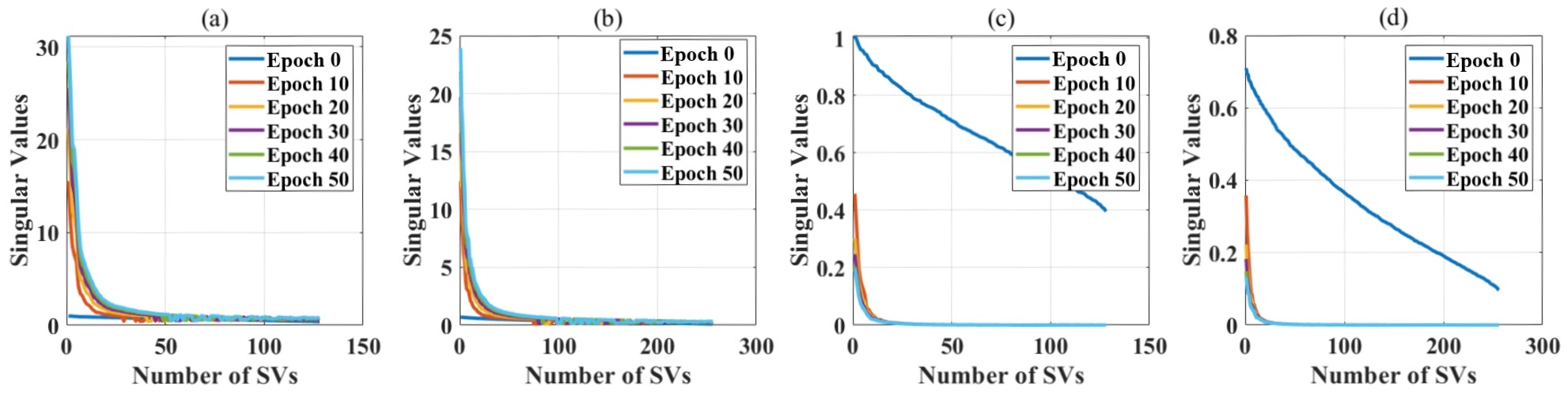
Figure 4: (a) and (b) show the trends of SVs of $\bm{W}^{(1)}\bm{W}^{(1)T}$ with and without regularizer, respectively. (c) and (d) show the trends of SVs of $\bm{W}^{(2)}\bm{W}^{(2)T}$ with and without regularizer, respectively. It is obvious that when the regularizer is included in the training process, SVs keeps decreasing as the number of training epochs increases.

V-B VBMF vs. NRMF

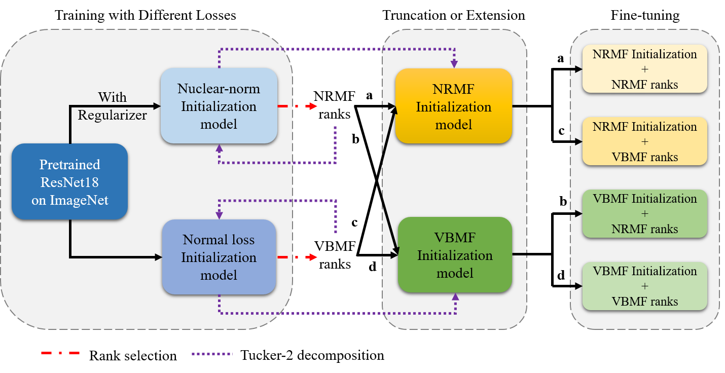
Figure 5: Experimental procedure in Section V-B. Firstly, we use the pretrained model on ImageNet to train on CIFAR-10 with and without nuclear-norm-like regularizer. Next, by applying VBMF and NRMF to the obtained normal and nuclear-norm initialization models separately, we can get VBMF and NRMF ranks. After this, we use the ranks to do the Tucker-2 decomposition as shown by the dotted arrows. Therefore, we collect VBMF and NRMF initialization models. Next, we use each of the two sets of the ranks on the VBMF and NRMF initialization models, such that a total of four rank-initialization combinations are obtained for the fine-tuning phase.

TABLE I: Threshold effects for ResNet18 on CIFAR-10 with $p=92\%$

	VBMF ranks	NRMF ranks
VBMF initialization	$94.40\%$	$93.50\%$
NRMF initialization	$95.46\%$	$94.21\%$
# Parameters	$7.01M$	$3.05M$

TABLE II: Threshold effects for ResNet18 on CIFAR-10 with $p=95\%$

	VBMF ranks	NRMF ranks
VBMF initialization	$94.40\%$	$94.40\%$
NRMF initialization	$93.58\%$	$93.91\%$
# Parameters	$7.01M$	$3.88M$

TABLE III: Threshold effects for ResNet18 on CIFAR-10 with $p=98\%$

	VBMF ranks	NRMF ranks
VBMF initialization	$94.40\%$	$95.07\%$
NRMF initialization	$92.98\%$	$93.58\%$
# Parameters	$7.01M$	$5.28M$

Here we compare the performances of VBMF-based and NRMF-based Tucker-2 decomposition via ResNet18 on CIFAR-10. The test setup and flow are depicted in Figure 5. As described in Section IV-C, the value of $p$ is important for determining the ranks. In order to explore the effect of $p$ on NRMF, we take $p=92\%,95\%,98\%$, and record the performances of NRMF under these three settings.

For clarity, here we elaborate what is done in the “Truncation or Extension” stage in Figure 5. Before this stage, we already have two different sets of ranks, namely, VBMF ranks and NRMF ranks. Correspondingly, we have two different initialization models. By regarding the VBMF and NRMF initialization models as the baselines, we can use VBMF and NRMF ranks to modify them. Paths a&d in Figure 5 can be understood as entering the fine-tuning stage using the NRMF (VBMF) ranks and NRMF (VBMF) truncated Tucker-2 factors. The operations of paths b&c are similar, and here we take path b as an example. Assume there is a CONV layer decomposed into three smaller ones of size $[1,1,128,100]$, $[3,3,100,120]$, and $[1,1,120,256]$ in VBMF initialization model, and the corresponding NRMF ranks of the given CONV layer are $110$ and $90$. Then we will modify the three CONV layers to $[1,1,128,110]$, $[3,3,110,90]$, and $[1,1,90,256]$ according to the NRMF ranks. This is done by padding zeros to the CONV layer of size $[1,1,128,100]$ and truncating the CONV layer of size $[3,3,120,256]$. As for the middle one of the three smaller CONV layers, padding and truncating operations are applied on the input and output channels, respectively.

It is shown in Tables III to III that NRMF provides higher compression ratios (viz. much smaller number of parameters) with little test accuracy loss. It is observed that the highest prediction accuracy is not achieved by the combination of NRMF ranks and initialization. One possible reason is that SVs in NRMF have been already squeezed to nearly zeros, and it is more difficult to bring them back to higher values for better accuracy via fine-tuning. We note that fine-tuning through path b using NRMF ranks reaches competitive precision with VBMF ranks at only half the parameters. Compared with the other two truncation ways, the NRMF initialization and ranks offer a graceful tradeoff between complexity and prediction accuracy. In the following experiments, we adopt the combination of VBMF initialization and NRMF ranks to demonstrate effectiveness of our rank selection method.

TABLE IV: Layer-wise analysis on ResNet18. $S$: input channel dimension, $T$: output channel dimension, $R_{3}$ and $R_{4}$ are Tucker-2 ranks. $p=95\%$ to select ranks.

Layer	$S/R_{3}$	$T/R_{4}$	#Parameters
conv1	$256$	$256$	$589.82K$
conv1 (VBMF)	$168$	$176$	$354.18K(\times 1.67)$
conv1 (NRMF)	$144$	$141$	$255.70K(\times 2.31)$
conv2	$256$	$512$	$1.18M$
conv2 (VBMF)	$194$	$275$	$670.61K(\times 1.76)$
conv2 (NRMF)	$222$	$299$	$807.32K(\times 1.46)$
conv3	$512$	$512$	$2.36M$
conv3 (VBMF)	$332$	$328$	$1.32M(\times 1.79)$
conv3 (NRMF)	$292$	$212$	$815.18K(\times 2.89)$
conv4	$512$	$512$	$2.36M$
conv4 (VBMF)	$348$	$342$	$1.42M(\times 1.66)$
conv4 (NRMF)	$160$	$69$	$216.61K(\times 10.89)$
conv5	$512$	$512$	$2.36M$
conv5 (VBMF)	$382$	$392$	$1.74M(\times 1.35)$
conv5 (NRMF)	$31$	$39$	$46.72K(\times 50.50)$

V-C Layer-wise Analysis of Compression Ratios

In this section, we present the layer-wise analysis of compression ratios via VBMF-based and NRMF-based Tucker-2 decomposition. We apply the two approaches to ResNet18 on CIFAR-10. As for the rank selection setting, we employ $p=95\%$. Besides, the number of epochs for fine-tuning is $50$ for both VBMF-based and NRMF-based compressed models. Furthermore, only the CONV layers with $3\times 3$ kernels are compressed, i.e., totally $16$ CONV layers in ResNet18. We do not compress CONV layers with $1\times 1$ kernels and fully connected layers. The number of parameters of those $16$ original CONV layers is $10.99M$. After compression, the number of parameters of those CONV layers becomes ${6.82M}$ and ${3.67M}$ for VBMF-based and NRMF-based compressed models, respectively. The accuracy of VBMF-based and NRMF-based compressed models are both $94.40\%$.

In Table IV, the layer-wise analyses of last five compressed CONV layers are presented. It is worth noting that for conv4 and conv5, NRMF has a clear advantage over VBMF. Especially for conv5, compared with the original CONV layer, the amount of parameters is reduced by $50.5\times$. Although VBMF performs better than NRMF on conv2, the gap between their compression ratios is small and can be ignored. Overall, NRMF achieves higher compression ratios on almost every layer, and can obtain a more compact model.

These results clearly show the advantages of dynamic rank search in NRMF over the fixed-rank approach in VBMF, and also the power of NRMF in revealing the unexploited data redundancy for deeper compression.

V-D Performances on Various Datasets and Neural Networks

Finally, NRMF is evaluated on CIFAR-10, CIFAR-100 and ImageNet with various CNNs. As before, we compare NRMF with the original networks and VBMF. We set $\alpha=10^{-2}$ as scaling of the nuclear-norm regularizer.

TABLE V: Performance comparison on CIFAR-10

Model	Rank Selection	Top-1 Accuracy (%)	#Parameters
AlexNet	Baseline	$91.85$	$57.04M$
	VBMF	$91.29$	$55.93M$
	NRMF	$91.03$	$55.05M$
GoogLeNet	Baseline	$95.53$	$5.61M$
	VBMF	$96.18$	$4.20M$
	NRMF	$95.57$	$4.08M$
DenseNet	Baseline	$96.56$	$6.96M$
	VBMF	$95.29$	$5.85M$
	NRMF	$96.99$	$5.85M$

CIFAR-10 and CIFAR-100 Table V presents the compression results of Tucker-2 decomposition with VBMF and NRMF ranks for AlexNet, GoogLeNet and DenseNet on CIFAR-10. It can be seen that NRMF offers the smallest models with little difference in accuracy. Surprisingly, the NRMF-compressed DenseNet is even better than the original, reaching $96.99\%$ prediction accuracy. Table VI shows the results for CIFAR-100, whereby similar observations can be made.

TABLE VI: Performance comparison on CIFAR-100

Model	Rank Selection	Top-1 Acc. (%)	Top-5 Acc. (%)	#Parameters
AlexNet	Baseline	$71.12$	$91.75$	$57.41M$
	VBMF	$69.73$	$90.51$	$56.32M$
	NRMF	$68.97$	$90.06$	$55.45M$
GoogLeNet	Baseline	$78.96$	$95.56$	$5.70M$
	VBMF	$79.50$	$95.88$	$4.27M$
	NRMF	$78.93$	$95.25$	$4.14M$
DenseNet	Baseline	$81.43$	$96.30$	$7.06M$
	VBMF	$82.98$	$96.13$	$5.92M$
	NRMF	$83.53$	$96.70$	$5.90M$

TABLE VII: Performance comparison on ImageNet

Model	Rank Selection	Top-1 Acc. (%)	Top-5 Acc. (%)	#Parameters
ResNet18	Base	$69.76$	$89.08$	$11.69M$
	VBMF	$67.20$	$87.88$	$7.50M$
	NRMF	$67.27$	$87.7$	$6.81M$

ImageNet For ResNet18 on ImageNet (ILSVRC2012), we present performance and comparison with VBMF ranks in Table VII. Again, NRMF achieves higher compression with fewer parameters and also higher top-1 accuracy.

Additionally, we verify there is high redundancy in the last two layers in ResNet18. By varying the learning rate to $10^{-3}$ in the training process adding our new loss, we get a set of ranks with small values using $p=95\%$. Similar to Table IV, we set ranks $S$, $T$ for the last two layers conv4, conv5 as $30$, $6$ and $6$, $31$ respectively. We then do Tucker-2 decomposition on the last two convolution layers and fine-tune. The number of parameters in the compressed model is $7.01M$, with top-1 and top-5 accuracies being $67.14\%$ and $87.49\%$, respectively. Compared to compressing all convolution layers using VBMF and NRMF ranks, factorizing only two layers can also provide similar levels of compression and performance.

VI Conclusion

We present nuclear-norm rank minimization factorization (NRMF) to exploit elasticity in the 4-way kernel tensor for CNN compression. For the first time, the ranks are dynamically found through a nuclear-norm regularizer during training, which can be perceived as a game between compression and prediction accuracy. Compared to the fixed-rank variational Bayesian matrix factorization (VBMF) approach, NRMF produces higher compression ratios in various CNN structures (viz. ResNet18, AlexNet, GoogLeNet and DenseNet). Perhaps more importantly, by observing the singular value dynamics, our scheme reveals the elasticity and redundancy patterns across CNN layers, thus providing insights and guidance in compressing specific layers.

References

- [1] Z. Wu, Y.-G. Jiang, J. Wang, J. Pu, and X. Xue, “Exploring inter-feature and inter-class relationships with deep neural networks for video classification,” in Proceedings of the 22nd ACM international conference on Multimedia, 2014, pp. 167–176.
- [2] Y. Liu, Y. Wang, S. Wang, T. Liang, Q. Zhao, Z. Tang, and H. Ling, “Cbnet: A novel composite backbone network architecture for object detection.” in AAAI, 2020, pp. 11 653–11 660.
- [3] S. Hong, H. Noh, and B. Han, “Decoupled deep neural network for semi-supervised semantic segmentation,” in Advances in neural information processing systems, 2015, pp. 1495–1503.
- [4] S. Han, H. Mao, and W. J. Dally, “Deep compression: Compressing deep neural network with pruning, trained quantization and huffman coding,” CoRR, vol. abs/1510.00149, 2016.
- [5] J. Cheng, J. Wu, C. Leng, Y. Wang, and Q. Hu, “Quantized cnn: A unified approach to accelerate and compress convolutional networks,” IEEE transactions on neural networks and learning systems, vol. 29, no. 10, pp. 4730–4743, 2017.
- [6] Y. Gong, L. Liu, M. Yang, and L. Bourdev, “Compressing deep convolutional networks using vector quantization,” arXiv preprint arXiv:1412.6115, 2014.
- [7] X. Yu, T. Liu, X. Wang, and D. Tao, “On compressing deep models by low rank and sparse decomposition,” in Proceedings of the IEEE Conference on Computer Vision and Pattern Recognition, 2017, pp. 7370–7379.
- [8] M. Jaderberg, A. Vedaldi, and A. Zisserman, “Speeding up convolutional neural networks with low rank expansions,” arXiv preprint arXiv:1405.3866, 2014.
- [9] V. Lebedev, Y. Ganin, M. Rakhuba, I. Oseledets, and V. Lempitsky, “Speeding-up convolutional neural networks using fine-tuned CP-decomposition,” arXiv preprint arXiv:1412.6553, 2014.
- [10] Y.-D. Kim, E. Park, S. Yoo, T. Choi, L. Yang, and D. Shin, “Compression of deep convolutional neural networks for fast and low power mobile applications,” arXiv preprint arXiv:1511.06530, 2015.
- [11] B. Baker, O. Gupta, N. Naik, and R. Raskar, “Designing neural network architectures using reinforcement learning,” arXiv preprint arXiv:1611.02167, 2016.
- [12] H. Cai, C. Gan, T. Wang, Z. Zhang, and S. Han, “Once for all: Train one network and specialize it for efficient deployment,” in International Conference on Learning Representations, 2020. [Online]. Available: https://arxiv.org/pdf/1908.09791.pdf
- [13] A. Novikov, D. Podoprikhin, A. Osokin, and D. P. Vetrov, “Tensorizing neural networks,” in Advances in neural information processing systems, 2015, pp. 442–450.
- [14] T. Garipov, D. Podoprikhin, A. Novikov, and D. Vetrov, “Ultimate tensorization: compressing convolutional and fc layers alike,” arXiv preprint arXiv:1611.03214, 2016.
- [15] M. Astrid and S.-I. Lee, “Cp-decomposition with tensor power method for convolutional neural networks compression,” in 2017 IEEE International Conference on Big Data and Smart Computing (BigComp). IEEE, 2017, pp. 115–118.
- [16] A. Saha, K. S. Ram, J. Mukhopadhyay, P. P. Das, and A. Patra, “Fitness based layer rank selection algorithm for accelerating cnns by candecomp/parafac (cp) decompositions,” in 2019 IEEE International Conference on Image Processing (ICIP). IEEE, 2019, pp. 3402–3406.
- [17] X. Chen, Z. He, and J. Wang, “Spatial-temporal traffic speed patterns discovery and incomplete data recovery via svd-combined tensor decomposition,” Transportation research part C: emerging technologies, vol. 86, pp. 59–77, 2018.
- [18] S. Nakajima, M. Sugiyama, S. D. Babacan, and R. Tomioka, “Global analytic solution of fully-observed variational bayesian matrix factorization,” Journal of Machine Learning Research, vol. 14, no. Jan, pp. 1–37, 2013.
- [19] M. A. Carreira-Perpinán and Y. Idelbayev, ““learning-compression” algorithms for neural net pruning,” in Proceedings of the IEEE Conference on Computer Vision and Pattern Recognition, 2018, pp. 8532–8541.
- [20] K. Ullrich, E. Meeds, and M. Welling, “Soft weight-sharing for neural network compression,” arXiv preprint arXiv:1702.04008, 2017.
- [21] J. Liu, Z. Xu, R. Shi, R. C. Cheung, and H. K. So, “Dynamic sparse training: Find efficient sparse network from scratch with trainable masked layers,” arXiv preprint arXiv:2005.06870, 2020.
- [22] T. G. Kolda and B. W. Bader, “Tensor decompositions and applications,” SIAM review, vol. 51, no. 3, pp. 455–500, 2009.
- [23] A. Krizhevsky, I. Sutskever, and G. E. Hinton, “Imagenet classification with deep convolutional neural networks,” in Advances in neural information processing systems, 2012, pp. 1097–1105.
- [24] C. Szegedy, W. Liu, Y. Jia, P. Sermanet, S. Reed, D. Anguelov, D. Erhan, V. Vanhoucke, and A. Rabinovich, “Going deeper with convolutions,” in Proceedings of the IEEE conference on computer vision and pattern recognition, 2015, pp. 1–9.
- [25] K. He, X. Zhang, S. Ren, and J. Sun, “Deep residual learning for image recognition,” in Proceedings of the IEEE conference on computer vision and pattern recognition, 2016, pp. 770–778.
- [26] G. Huang, Z. Liu, L. Van Der Maaten, and K. Q. Weinberger, “Densely connected convolutional networks,” in Proceedings of the IEEE conference on computer vision and pattern recognition, 2017, pp. 4700–4708.
- [27] A. Krizhevsky, G. Hinton et al., “Learning multiple layers of features from tiny images,” 2009.
- [28] J. Deng, W. Dong, R. Socher, L.-J. Li, K. Li, and L. Fei-Fei, “Imagenet: A large-scale hierarchical image database,” in 2009 IEEE conference on computer vision and pattern recognition. Ieee, 2009, pp. 248–255.
- [29] Y. LeCun, C. Cortes, and C. Burges, “Mnist handwritten digit database,” ATT Labs [Online]. Available: http://yann.lecun.com/exdb/mnist, vol. 2, 2010.