Phase-space simulations of feedback coherent Ising machines

Abstract

A new technique is demonstrated for carrying out exact positive-P phase-space simulations of the coherent Ising machine quantum computer. By suitable design of the coupling matrix, general hard optimization problems can be solved. Here, computational quantum simulations of a feedback type of photonic parametric network are carried out, which is the implementation of the coherent Ising machine. Results for success rates are obtained using this scalable phase-space algorithm for quantum simulations of quantum feedback devices.

A wide variety of computational problems can be mapped to the problem of finding the ground state of an Ising model [1, 2]. These can be solved with a coherent Ising machine (CIM), a network of degenerate parametric oscillators (DPOs) operating above their threshold level, where a single Ising spin is represented by the in-phase amplitude of the DPO [3, 4, 5, 6, 7, 8]. There are two well-established schemes for a DPO-based CIM: one using coherent optical coupling and one using Field Programmable Gate Array (FPGA)-based measurement-feedback, as treated here. Each has distinct advantages and disadvantages [9]. Feedback methods have led to the development of large photonic quantum computational devices, with 100,000 nodes being recently demonstrated [10].

A fundamental question is how likely and how fast the CIM will find its energetic ground state. We wish to analyze this problem from a fully quantum physical standpoint, where quantum tunneling is potentially beneficial to the system’s performance. For this purpose, it is essential to develop phase-space simulations, which have been shown to be a very effective tool for the simulation of large quantum systems and optical quantum computers [11]. Recent examples of this include up to $16,000$ mode simulations of boson sampling networks [12].

An open quantum system is described by a master equation as a result of the system Hamiltonian and non-unitary (Lindblad) terms due to environment interactions. This master equation is converted into a Fokker-Planck equation (FPE) in phase-space methods (usually a positive-P or Wigner representation), the solution of which can then be approximated via sampling its equivalent stochastic differential equation (SDE).

When the system involves feedback that is conditional on measurement, the conditional master equation contains stochastic terms. These are due to the quantum noise associated with the monitored observable. These carry over to the Fokker-Planck equation, resulting in a stochastic Fokker-Planck equation (SFPE). This cannot immediately be converted into a set of SDEs, although a weighted approach is possible [13]. However, in simulating the CIM, one is most interested in the success probability obtained from the total feedback master equation [14, 15], which does not require weight terms.

It is important to note that the inclusion of quantum feedback may change the system dynamics profoundly, depending on the specific parameters. The literature describing systems involving continuous measurements with simulations via phase-space methods is quite limited, despite the prominence of feedback control as an experimental technique[16]. Other methods exist for small quantum systems, but the phase-space techniques are the only ones that have reached large sizes. We have identified an efficient method in the treatment of quantum feedback, and applied it to the CIM quantum computer.

An Ising machine is a physical model consisting of a set of effective spins $\sigma\left(i\right)$, where $\sigma\left(i\right)\in\left\{-1,1\right\}$ with a set of (real-valued) weights $J_{ij}\in\mathbb{R}$. The system is designed to reach the ground state of an Ising Hamiltonian:

$$\mathcal{H}_{IM} = -\sum_{i,j}J_{ij}\sigma\left(i\right)\sigma\left(j\right)\,.$$ (1)

To obtain a nearly equivalent experimental model, a driven and damped feedback network is used. Each node $j$ is a degenerate optical parametric oscillator (DOPO) [17, 18, 19, 20], treated here as an optical cavity that contains two modes $a$ (the signal mode) and $a_{p}$ (the pump mode), where in our case $\omega_{p}=2\omega_{s}$. In the rotating reference frame, the Hamiltonian is

$$\mathcal{H} = \mathcal{H}_{int}+\mathcal{H}_{pump}+\mathcal{H}_{loss},$$ (2)

where $\mathcal{H}_{int},\mathcal{H}_{pump},\mathcal{H}_{loss}$ denote the interaction, pump and loss terms, respectively and

$$\mathcal{H}_{int} = \frac{i\hbar\kappa}{2}\left[\left(a^{\dagger}\right)^{2}a_{p}-a^{2}a_{p}^{\dagger}\right]$$

$$\mathcal{H}_{pump} = i\hbar\left[\epsilon_{p}a_{p}^{\dagger}-\epsilon_{p}^{*}a_{p}\right]$$ (3)

Here $\epsilon_{p}$ is the pump field amplitude and $\kappa$ denotes the non-linear interaction [21].

As well as the usual pump and loss terms common to equations of this type, the experiment requires a coupling between the oscillators in order to implement an Ising-like model, which includes a feedback loop. This enables the output of one DOPO to be used to modify the pump rate in the other oscillators. The overall effect of this leads to an Ising-like coupling between the oscillators. A feedback-controlled system such as the DOPO network studied here therefore requires a measurement carried out continuously on its system state. Considering the state collapse that comes with every measurement on a quantum system, it is not obvious at all how a continuous measurement, resulting in a “continuous state collapse” can be described mathematically.

This question has been addressed in the quantum optics literature [22, 23, 14, 24, 25, 26], with later extensions [13]. One considers a monitored quantum system described by a conditional density operator $\rho_{c}$, that depends on a set of measurement outcomes. A feedback master equation in the Ito stochastic calculus is obtained. A measurement noise is generated during a specific realization of the measurement. However, we are more interested in the system evolution averaged over all possible measurement noise realizations, which is described by the much simpler total master equation.

For this case, we recursively extend the single homodyne detection result[24] to treat multiple feedback loops, giving:

$$\dot{\rho}=\mathcal{L}\rho+\sum_{j}\mathcal{K}_{j}\left(a_{j}\rho+\rho a_{j}^{\dagger}\right)+\frac{1}{4\gamma_{m}}\sum_{\mu}\mathcal{K}_{j}^{2}\rho.$$ (4)

Here $\mathcal{L}\rho$ described unmonitored evolution and total damping, while the $\mathcal{K}_{j}$ super-operators describe the feedback of the measured quadrature $X_{j}=a_{j}+a_{j}^{\dagger}$ onto the system, with a corresponding amplitude decay rate of $\gamma_{m}$ including measurement efficiency factors.

This averages the conditional Ito master equation over all the noises, which is equivalent to setting the noise terms to zero [14, 15], owing to the factorization properties of Ito stochastic equations combined with the linearity of the stochastic master equation as a function of $\rho_{c}$.

We take the $j$-th feedback super-operator $\mathcal{K}_{j}$ to be:

$$\mathcal{K}_{j}\rho=\zeta\sum_{i}J_{ij}\left[a_{i}^{\dagger}-a_{i},\rho\right]\,,$$ (5)

where $\zeta$ is a feedback factor, and $J_{ij}$ is the Ising model matrix. Combining this feedback treatment with the theory of each single degenerate optical parametric oscillator [17], the simplest quantum model of the $N$-node CIM is therefore described by the total master equation

$$\frac{d\rho}{dt} = \sum_{i}\left\{\gamma\left(2a_{i}\rho a_{i}^{\dagger}-a_{i}^{\dagger}a_{i}\rho-\rho a_{i}^{\dagger}a_{i}\right)\right.$$ (6)

$$+\gamma_{p}\left(2a_{pi}\rho a_{pi}^{\dagger}-a_{pi}^{\dagger}a_{pi}\rho-\rho a_{pi}^{\dagger}a_{pi}\right)$$

$$+\left[\epsilon_{pi}a_{pi}^{\dagger}-h.c,\rho\right]+\frac{1}{4\gamma_{m}}\mathcal{K}_{i}^{2}\rho$$

$$\left.+\frac{\kappa}{2}\left[\left(a_{i}^{\dagger}\right)^{2}a_{pi}-a_{i}^{2}a_{pi}^{\dagger},\rho\right]+\mathcal{K}_{i}\left(a_{i}\rho+\rho a_{i}^{\dagger}\right)\right\}\,.$$

The signal and pump modes $a_{i}$ and $a_{pi}$ are associated with unmonitored decay rates $\gamma_{s},\gamma_{p}$, respectively. There is an additional system parameter $\gamma_{m}$, representing measurement of the signal mode, while $\gamma$ is the total decay rate including measurement loss, and $\mathcal{K}_{j}$ is the feedback super-operator given above. The second-order term in $\mathcal{K}_{j}$ in (6) accounts for the quantum diffusion introduced by the injection of quantum noise during the feedback process, and is an important source of decoherence.

The pump strength $\epsilon_{pi}$ is independent of the signal amplitude and will generally be set as uniform for all DOPOs ($\epsilon_{pi}=\epsilon_{p}$). The action of the feedback term in Eq. (6) is similar to inducing a signal input $\hat{\epsilon}_{i}$ which results from continuous homodyne detection via

$$\hat{\epsilon}_{i} = \zeta\sum_{j}J_{ij}\hat{X}_{j}\,,$$ (7)

where $\hat{X}_{j}=a_{j}^{\dagger}+a_{j}$ is the measured quadrature for DOPO site $j$. It is also subject to measurement quantum noise, but this averages to zero for the total master equation, and is therefore omitted in such equations.

While master equations can be treated directly using a number state expansion, the exponentially large size of the Hilbert space makes this computationally prohibitive for large network experiments. This necessitates alternative approaches to simulation.

One approach is to include measurement noise terms, giving a conditional master equation. This does not translate into a standard FPE, but to a stochastic Fokker-Planck equation (SFPE), which cannot be converted into a conventional stochastic differential equation (SDE). The noise terms associated with the measurement are different in nature to the familiar noise terms one typically encounters for the integration of SDEs. In the literature, these measurement noise terms are often called “physical” noise. The approach used in some earlier papers is to use weighted phase-space trajectories to treat them. While this allows a detailed understanding of the measurement noise, it reduces the simulation efficiency.

Here we describe an exact phase-space method that maps the total quantum master equation into intuitively understandable and readily simulated stochastic equations. This ignores the conditional current, but it reliably gives the average final state of the system. Therefore, Eq. (6) can be very efficiently treated using phase-space methods. The total feedback master equation requires no additional weighting terms, and is especially suitable for treating very large quantum feedback systems, due to its greater scalability. Taking an average over the measurement noise does not change the overall master equation or the success rate of the CIM.

The positive-P phase-space representation [27] gives an exact method for integrating such master equations provided boundary terms vanish. This requires that the probabilities decay rapidly enough at large radius in phase-space [28], which is well-satisfied here. Another method, the truncated Wigner method[29, 30], truncates terms of O($N^{-3/2})$ in an expansion in the photon number $N$, to obtain a positive-valued distribution. Due to the small number of photons at the initial stages of the experiment, we use the more accurate positive-P approach instead.

Eq. (6) results in the Fokker-Planck equation (FPE) for the positive-P representation:

$$\frac{dP}{dt}=\sum_{i}\left[\mathcal{D}_{i}-2\zeta\sum_{j}J_{ij}\partial_{x_{i}}\left[x_{j}-\frac{\zeta}{2\gamma_{m}}\sum_{k}J_{kj}\partial_{x_{k}}\right]\right]P\,.$$ (8)

Here, $\mathcal{D}_{i}$ is the standard OPO Fokker-Planck equation for a single device, with the damping rate given by $\gamma$, and we define $x_{j}\equiv\alpha_{j}+\beta_{j}$ and $\partial_{x_{i}}\equiv\left(\partial_{\alpha_{i}}+\partial_{\beta_{i}}\right)/2$. The resulting Ito stochastic differential equations are:

$$\dot{\alpha}_{i} = \epsilon_{i}-\gamma\alpha_{i}+\kappa\beta_{i}\alpha_{pi}+\sqrt{\kappa\alpha_{pi}}\xi_{i}^{\alpha}$$

$$\dot{\beta}_{i} = \epsilon_{i}-\gamma\beta_{i}+\kappa\alpha_{i}\beta_{pi}+\sqrt{\kappa\beta_{pi}}\xi_{i}^{\beta}$$

$$\dot{\alpha}_{pi} = \epsilon_{p}-\gamma_{p}\alpha_{pi}-\frac{\kappa}{2}\alpha_{i}^{2}$$

$$\dot{\beta}_{pi} = \epsilon_{p}-\gamma_{p}\beta_{pi}-\frac{\kappa}{2}\beta_{i}^{2}\,.$$ (9)

The stochastic feedback term $\epsilon_{i}$ includes both a coherent term and a noise term coming from the second order derivative terms in the Fokker-Planck equation, so that:

$$\epsilon_{i}\equiv\zeta\sum_{j}J_{ij}\left(\alpha_{j}+\beta_{j}+\frac{1}{\sqrt{2\gamma_{m}}}\xi_{j}\right),$$ (10)

where $\xi_{i}^{\alpha}$, $\xi_{i}^{\beta}$, $\xi_{i}$ are delta-correlated Gaussian noise increments.

Next, we look at the adiabatically eliminated SDEs in Eq. (9), obtained by setting $\dot{\alpha}_{pi}=\dot{\beta}_{pi}=0$ in the Ito stochastic equations [17, 31]. Identical results are obtained, although with greater complexity, using operator adiabatic methods within the master equation [32]. We introduce an effective nonlinearity, $\chi\left(\alpha\right)\equiv\kappa\left[\epsilon_{p}-\frac{\kappa}{2}\alpha^{2}\right]/\gamma_{p}$ , and utilize this to find the stochastic differential equations. For greater efficiency in numerical integration [33], these can be transformed into their equivalent Stratonovich form. This modifies the damping rate so that $\gamma\rightarrow\gamma^{\prime}\equiv\gamma-\kappa^{2}/4\gamma_{p}\,$, giving:

$$\dot{\alpha}_{i} = \epsilon_{i}-\gamma^{\prime}\alpha_{i}+\beta_{i}\chi\left(\alpha_{i}\right)+\sqrt{\chi\left(\alpha_{i}\right)}\xi_{i}^{\alpha}$$

$$\dot{\beta}_{i} = \epsilon_{i}-\gamma^{\prime}\beta_{i}+\alpha_{i}\chi\left(\beta_{i}\right)+\sqrt{\chi\left(\beta_{i}\right)}\xi_{i}^{\beta}\,.$$ (11)

The stochastic nature of the feedback noise is included in the feedback term $\epsilon_{i}$, while $\xi_{i}^{\alpha,\beta}$ are internal quantum noise terms that generate non-classical squeezing and entanglement.

We first consider an experiment with 2 coupled DOPOs. Here, the interaction matrix $\mathbf{J}$ is simply $J_{ij}=\left(\delta_{ij}-1\right)$, corresponding to antiferromagnetic coupling. The experiment is initialized with both cavity modes $a_{1,2}$ in the vacuum state. During the simulation time, which extends from $0$ to $T_{max}=100$, the pump strength $\epsilon_{p}$ is linearly increased from $0$ to $2\cdot\epsilon_{th}$, where $\epsilon_{th}=\gamma\gamma_{p}/\kappa$ is the threshold pump strength. This way, the system is gradually steered from a below-threshold to an above-threshold region where different spin configurations correspond to local minima in the energy landscape. A gradual transition increases the likelihood of finding a global minimum corresponding to the two degenerate ground states of the Ising system simulated here, closely resembling a simulated annealing process. The system parameters are $\gamma=1.1$, $\gamma_{p}=100$, $\kappa=0.316227$, $\gamma_{m}=0.1$, $\zeta=0.3$. For the positive-P integration, we used a hierarchy of $N_{e}\times N_{s}$ ensembles, in order to calculate the sampling errors [34], with $N_{s}=8192$ subensemble samples and $N_{t}=50\cdot 10^{3}$ time-steps. We integrated the system dynamics according to Eqs. (11) using a stochastic RK4 scheme. The simulations were run on a computer cluster using multiple GPUs and implemented in C++ using CUDA. An independent check was carried out using a public domain stochastic integration code [34, 35], with identical results. Discretization error and sampling errors were checked, and found to be negligible. We define a success rate as the number of quantum trajectories that adopt one of the two degenerate ground states of the antiferromagnetic Ising model divided by the total number of quantum trajectories. The ground states are indicated by the sign signatures $\left(+,-\right)$ and $\left(-,+\right)$ for the $x$-quadratures of the cavity modes $a_{1,2}$. A success rate of $1$ is obtained for $100\times 8192$ independent repetitions of the simulation.

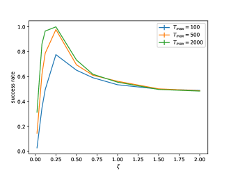
Figure 1: Simulation results for the 16-DOPO experiment, showing the success rate for two different integration times and a range of interaction parameters $\zeta$. The results were obtained using the positive-P scheme, using $20\times 8192$ independent simulations at each data point for $T_{max}=100$, $T_{max}=500$ and $T_{max}=2000$, respectively.

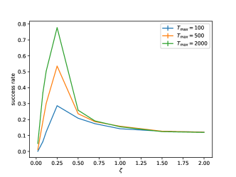
Figure 2: Simulation results for the 32-DOPO experiment, showing the success rate for two different integration times and a range of interaction parameters$\zeta$, using $20\times 8192$ independent simulations at each data point.

We also considered two larger experiments, consisting of $N=16$ and $N=32$ DPO cavities, respectively, which are more realistic cases. The cavities are coupled antiferromagnetically through nearest neighbor interaction in a circular sense where $\mathbf{J}$ is given by $J_{ij}=-1$ if $\left|i-j\right|=1$ or $\left|i-j\right|=N-1$, $J_{ij}=0$ otherwise. The ground states have sign signatures $\left(+,-,...,+,-\right)$ and $\left(-,+,...,-,+\right)$ for the $x$-quadratures of $a_{1},...,a_{N}$.

The parameters $\gamma$, $\gamma_{p}$, $\kappa$, $\gamma_{m}$, $N_{S}$, $N_{t}$ are the same as in the $N=2$ case, however, the interaction strength $\zeta$ is varied. We also use three different integration times $T_{max}$ to demonstrate its effect on the simulation efficacy of the simulated coherent Ising machine. We integrate the system dynamics and determine the success rate analogously to the $N=2$ case, which is plotted against the interaction strength $\zeta$ for a fixed integration time $T_{max}$. We have simulated $9$ different values for $\zeta$. The results are shown in Figs. 1 and 2. Generating all data points for $T_{max}$ and $\zeta$ takes about 1 hour, when utilizing 10 GPUs (NVIDIA P100).

From these results, very high success rates close to $1$ can be achieved with the right choice of $T_{max}$ and $\zeta$, although this requires further investigation into different types of optimization problem. Longer simulation times, with an adiabatic increase of the pump field, result in a higher success rate. These simulations also allow other types of sweep to be investigated. Somewhat counter-intuitively, a strong feedback coupling does not always improve the results, and in may reduce the success rate. This appears to be caused by the quantum feedback noise introducing errors due to random jumps between the near ground-state solutions, resulting in an effective thermalization of the steady-state. Between the $N=16$ and $N=32$ case, the success rate is reduced significantly, especially for non-optimal values of $\zeta$. A decrease of the success rate with increasing problem size is consistent with previous findings for similar CIM systems.

In conclusion, we have derived and implemented a numerical scheme for accurately simulating the coherent Ising machine in a feedback implementation. The innovation terms are treated in a fully mathematically justified way, proven to yield the exact expectation values in the limit of a large number of independent simulations. This will be an even more important feature when dealing with increasingly nonclassical cases. Since the methods are exact, they can be used as benchmarks for developing faster or more accurate algorithms in future. We note that a large variety of parameter values and sweep types are possible. These will be the subject of subsequent investigations.

References

- Lucas [2014] A. Lucas, Frontiers in Physics 2, 5 (2014).
- Pakin [2017] S. Pakin, in Proceedings of the Second International Workshop on Post Moores Era Supercomputing, PMES’17 (Association for Computing Machinery, New York, NY, USA, 2017) pp. 30–36.
- Wang et al. [2013] Z. Wang, A. Marandi, K. Wen, R. L. Byer, and Y. Yamamoto, Physical Review A 88, 063853 (2013).
- Marandi et al. [2014] A. Marandi, Z. Wang, K. Takata, R. L. Byer, and Y. Yamamoto, Nature Photonics 8, 937 (2014).
- Shoji et al. [2017] T. Shoji, K. Aihara, and Y. Yamamoto, Physical Review A 96, 053833 (2017).
- Yamamura et al. [2017] A. Yamamura, K. Aihara, and Y. Yamamoto, Physical Review A 96, 053834 (2017).
- McMahon et al. [2016] P. L. McMahon, A. Marandi, Y. Haribara, R. Hamerly, C. Langrock, S. Tamate, T. Inagaki, H. Takesue, S. Utsunomiya, K. Aihara, R. L. Byer, M. M. Fejer, H. Mabuchi, and Y. Yamamoto, Science 354, 614 (2016).
- Inagaki et al. [2016] T. Inagaki, Y. Haribara, K. Igarashi, T. Sonobe, S. Tamate, T. Honjo, A. Marandi, P. L. McMahon, T. Umeki, K. Enbutsu, O. Tadanaga, H. Takenouchi, K. Aihara, K.-i. Kawarabayashi, K. Inoue, S. Utsunomiya, and H. Takesue, Science 354, 603 (2016).
- Yamamoto et al. [2017] Y. Yamamoto, K. Aihara, T. Leleu, K.-i. Kawarabayashi, S. Kako, M. Fejer, K. Inoue, and H. Takesue, npj Quantum Information 3, 49 (2017).
- Honjo et al. [2021] T. Honjo, T. Sonobe, K. Inaba, T. Inagaki, T. Ikuta, Y. Yamada, T. Kazama, K. Enbutsu, T. Umeki, R. Kasahara, et al., Science advances 7, eabh0952 (2021).
- D Drummond and Chaturvedi [2016] P. D Drummond and S. Chaturvedi, Physica scripta 91, 73007 (2016).
- Drummond et al. [2021] P. D. Drummond, B. Opanchuk, A. Dellios, and M. D. Reid, arXiv preprint arXiv:2102.10341 (2021).
- Hush et al. [2009] M. R. Hush, A. R. R. Carvalho, and J. J. Hope, Physical Review A 80, 013606 (2009).
- Wiseman and Milburn [1993] H. M. Wiseman and G. J. Milburn, Physical Review Letters 70, 548 (1993).
- Bushev et al. [2006] P. Bushev, D. Rotter, A. Wilson, F. Dubin, C. Becher, J. Eschner, R. Blatt, V. Steixner, P. Rabl, and P. Zoller, Physical review letters 96, 043003 (2006).
- Zhang et al. [2017] J. Zhang, Y. xi Liu, R.-B. Wu, K. Jacobs, and F. Nori, Physics Reports 679, 1 (2017), quantum feedback: theory, experiments, and applications.
- Drummond et al. [1981] P. Drummond, K. McNeil, and D. Walls, Optica Acta: International Journal of Optics 28, 211 (1981).
- Sun et al. [2019a] F.-X. Sun, Q. He, Q. Gong, R. Y. Teh, M. D. Reid, and P. D. Drummond, New Journal of Physics 21, 093035 (2019a).
- Sun et al. [2019b] F.-X. Sun, Q. He, Q. Gong, R. Y. Teh, M. D. Reid, and P. D. Drummond, Physical Review A 100, 033827 (2019b).
- Teh et al. [2020] R. Y. Teh, F.-X. Sun, R. E. S. Polkinghorne, Q. Y. He, Q. Gong, P. D. Drummond, and M. D. Reid, Physical Review A 101, 043807 (2020).
- Drummond and Hillery [2014] P. D. Drummond and M. Hillery, The quantum theory of nonlinear optics (Cambridge University Press, 2014).
- Caves and Milburn [1987] C. M. Caves and G. J. Milburn, Physical Review A 36, 5543 (1987).
- Dalibard et al. [1992] J. Dalibard, Y. Castin, and K. Mølmer, Physical Review Letters 68, 580 (1992).
- Wiseman [1994] H. M. Wiseman, Physical Review A 49, 2133 (1994).
- Jacobs and Steck [2006] K. Jacobs and D. A. Steck, Contemporary Physics 47, 279 (2006).
- Wiseman and Milburn [2009] H. M. Wiseman and G. J. Milburn, Quantum Measurement and Control (Cambridge University Press, 2009).
- Drummond and Gardiner [1980] P. D. Drummond and C. W. Gardiner, Journal of Physics A: Mathematical and General 13, 2353 (1980).
- Gilchrist et al. [1997] A. Gilchrist, C. W. Gardiner, and P. D. Drummond, Physical Review A 55, 3014 (1997).
- Wigner [1932] E. Wigner, Phys. Rev. 40, 749 (1932).
- Drummond and Hardman [1993] P. D. Drummond and A. D. Hardman, Europhysics letters 21, 279 (1993).
- Gardiner [1984] C. Gardiner, Physical Review A 29, 2814 (1984).
- Carmichael [2009] H. J. Carmichael, Statistical methods in quantum optics 2: Non-classical fields (Springer Science & Business Media, 2009).
- Drummond and Mortimer [1991] P. Drummond and I. Mortimer, Journal of computational physics 93, 144 (1991).
- Kiesewetter et al. [2016] S. Kiesewetter, R. Polkinghorne, B. Opanchuk, and P. D. Drummond, SoftwareX 5, 12 (2016).
- Opanchuk et al. [2018] B. Opanchuk, L. Rosales-Zárate, M. D. Reid, and P. D. Drummond, Physical Review A 97, 042304 (2018).