Three-$\alpha$ configurations in the $0^{+}$ states of ${}^{12}\mathrm{C}$

Abstract

Geometric configurations of three-$\alpha$ particles in the ground- and first-excited $J^{\pi}=0^{+}$ states of ¹²C are discussed within two types of $\alpha$-cluster models which treat the Pauli principle differently. Though there are some quantitative differences especially in the internal region of the wave functions, equilateral triangle configurations are dominant in the ground state, while in the first excited $0^{+}$ state isosceles triangle configurations dominate, originating from ${}^{8}{\rm Be}+\alpha$ configurations.

1 Introduction

An $\alpha$ (⁴He nucleus) clustering phenomenon is one of the most important aspects of nuclear physics. In particular, the first excited $J^{\pi}=0^{+}$ state, $0_{2}^{+}$, the so-called Hoyle state has attracted attention as it plays a crucial role in the nucleosynthesis h54 and in a context of the Bose-Einstein condensed (BEC) state THSR . Motivated by the recent progress in the structure study based on algebraic cluster models f19 ; vcfl20 , here we discuss geometric configurations of $\alpha$ particles in the $0_{1}^{+}$ and $0_{2}^{+}$ states of ¹²C using precise three-$\alpha$ wave functions. In this paper, we treat the $\alpha$ particle as a point particle. To incorporate the Pauli principle between two $\alpha$ particles, two types of potential models are employed: the orthogonality condition model OCM and the shallow potential model ab65 . In the orthogonality condition model, the Pauli principle is taken into account by imposing the orthogonality condition on the Pauli forbidden states for the relative motion between $\alpha$ particles. The resulting radial wave function is pushed out, exhibiting some nodes in the internal region. In the shallow potential model, instead of using the orthogonality condition, a repulsive component at short distances is introduced to push the internal wave function out. It is known that those two phase-shift equivalent potentials give quite different results for some observables Pinilla11 ; Arai18 . We will discuss how these model difference affects the geometric configurations in the low-lying $0^{+}$ states of ¹²C.

2 Results and discussion

We start from a standard three-$\alpha$ Hamiltonian that consists of the kinetic, two-$\alpha$, and three-$\alpha$ potential terms. The Coulomb potential is included. For the OCM, we adopt the same Hamiltonian used in Ref. kk05 ; kk07 . This potential is deep enough to accommodate three redundant forbidden states. To exclude the Pauli forbidden states between $\alpha$ particles, we impose the orthogonality condition practically by adding a pseudo-potential to the Hamiltonian Kukulin78 . As a shallow potential model, we employ a slightly modified version of the Ali-Bodmer potential (AB) ab65 (Set a^′ Fedorov96 ), which is $l$-dependent and widely used to describe the Hoyle state i13 ; i14 ; nnt13 .

A three-$\alpha$ wave function $\Psi_{3\alpha}$ is described as a superposition of symmetrized correlated Gaussians with the aid of the stochastic variational method vs95 ; SVM . Details of the basis optimization can be found in Ref. LNP20 . Also see, e.g., Refs. Suzuki08 ; Mitroy13 ; Suzuki17 , for many examples showing the power of this approach. For the OCM, the calculated energy and the root-mean-square (rms) point-$\alpha$ radius of the $0_{1}^{+}$ ($0_{2}^{+}$) state are $-7.13$ (0.78) MeV and $1.73$ (4.58) fm, respectively. For the AB, the values are $-6.67$ (0.38) MeV and 1.84 (3.39) fm, respectively. These results are consistent with the ones obtained in Refs. ofkh13 ; i13 , respectively.

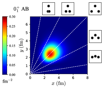
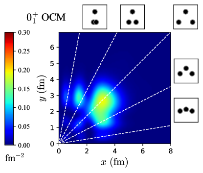
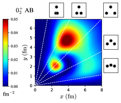
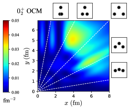
Figure 1: Two-body density distributions for $0_{1}^{+}$ and $0_{2}^{+}$ with the AB and OCM. The white dashed lines are plotted as guide for some specific geometric configurations that are illustrated in the boxes at the end of the lines, e.g., the diagonal line corresponds to the equilateral triangle configuration.

To discuss the configurations of three-$\alpha$ particles, we calculate the two-body density distributions (TBD), $\rho(x,y)=\left<\Psi_{3\alpha}\left|\delta(|\bm{x}_{1}|-x)\delta(|\bm{x}_{2}|-y)\right|\Psi_{3\alpha}\right>,$ where $\bm{x}_{1}=\bm{r}_{1}-\bm{r}_{2}$ and $\bm{x}_{2}=(\bm{r}_{1}+\bm{r}_{2})/2-\bm{r}_{3}$. Note $\int_{0}^{\infty}dx\int_{0}^{\infty}dy\,\rho(x,y)=1$. Figure 1 plots the TBD of $0_{1}^{+}$ and $0_{2}^{+}$ obtained by the AB and OCM. For $0_{1}^{+}$, the TBD for the AB simply has only one peak at the equilateral triangle shape, while for the OCM, the TBD shows other peak structures in regions of acute- and obtuse-isosceles triangles. In the OCM, several small peaks appear in the internal region, which come from the orthogonality condition on the Pauli forbidden states imposed in the solution of the OCM. On the other hand, for the AB, no peak is found due to the repulsive component contained in the AB potential. For $0_{2}^{+}$, the TBD is much extended and shows more complicated structures. For the AB, the TBD has predominantly two peaks in the equilateral and acute-isosceles triangle regions. The highest peak is located at the acute-isosceles triangles which implies the ${}^{8}\mathrm{Be}+\alpha$ configuration. For the OCM, though there are several peaks in the internal region due to the orthogonality condition, the dominant configurations are isosceles triangles, almost equal contributions from the acute- and obtuse-isosceles triangles.

Here we compare the wave function components for those two different $\alpha$ cluster models. Since the two models treat the Pauli principle differently, it is interesting to see the occupation probability of the harmonic oscillator quanta in the wave functions Suzuki96 ; hs14 . Figures 2 (a) and (b) plot the occupation probabilities for $0_{1}^{+}$ with the OCM and AB, respectively. According to the SU(3) limit of the three-$\alpha$ clusters Smirnov74 , the allowed state is $Q\geq 8$. In fact, for the OCM no forbidden state component with $Q<8$ and the $Q=8$ state is dominant, which is consistent with the result given in Ref. ys05 . In contrast, for the AB, the distribution shows quite different behavior: It is peaked at $Q=6$ and spreads, having contributions of $Q<8$. Figures 2 (c) and (d) show the occupation probabilities for $0_{2}^{+}$. Similarly to the $0_{1}^{+}$ case, no forbidden state component with $Q<8$ is included in the OCM, while they are found in the AB. Though there are some quantitative differences in the peak positions, the global behavior of the occupation probabilities are similar reflecting the characteristic behavior of well-developed cluster states Suzuki96 ; Neff12 ; hs14 ; Horiuchi14 .

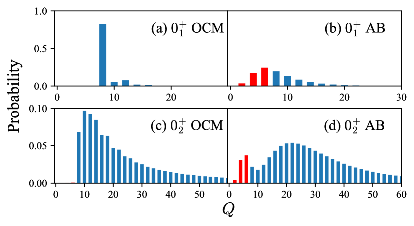
Figure 2: Occupation probabilities of the harmonic oscillator quanta $Q\hbar\omega$ for (a), (b) $0_{1}^{+}$ and (c), (d) $0_{2}^{+}$. The oscillator energy $\hbar\omega$ is set to be $22~{}\mathrm{MeV}$, consistently with the size parameter of the forbidden states used in the OCM. The states that are forbidden in the OCM ($Q=0$–6) are colored in red.

To corroborate the discussion, we list in Tab. 1 the probability of finding partial wave $(l)$ components between the two-$\alpha$ particles in the three-$\alpha$ system, $P_{l}$. In the OCM, $l=0,2,$ and 4 components are almost equal for $0_{1}^{+}$. This again confirms the SU(3) character of the wave function ys05 . Reminding $Q=2n+l=8$ with $n$ being the number of nodes, the dominant $Q=8$ component induces, e.g,. four nodes with $l=0$. For the AB, differently from the OCM result, the $0_{1}^{+}$ state is $l=0$ dominance. For $0^{+}_{2}$, $P_{l=0}$ is dominant for both the OCM and AB, which is consistent with the $\alpha$ condensed picture ys05 ; Yamada12 in which the three-$\alpha$ particles are occupied in the lowest orbit as bosons.

Table 1: Probability of finding partial wave $(l)$ components for $0_{1}^{+}$ and $0_{2}^{+}$ with the OCM and AB. The values in parenthesis are the spectroscopic factor of ${}^{8}{\rm Be}+\alpha$.

		$P_{l=0}$	$P_{l=2}$	$P_{l=4}$
$0_{1}^{+}$	OCM	$0.295$ (0.195)	0.348	0.313
	AB	$0.704$ (0.448)	0.294	0.001
$0_{2}^{+}$	OCM	$0.693$ (0.693)	0.141	0.087
	AB	$0.886$ (0.729)	0.108	0.003

These differences are also well reflected in the one-body density distribution (OBD) defined as $\rho(r)=\braket{\Psi_{3\alpha}}{\delta(}{\bm{r}_{1}-\bm{r}_{\rm cm}|-r)|\Psi_{3\alpha}}$, where $\bm{r}_{\rm cm}$ denotes the center-of-mass coordinate. Figure 3 (a) plots the OBD in the coordinate space. For $0_{1}^{+}$ with the OCM, as we see in the TBD, the OBD also exhibits some nodes in the internal region due to the orthogonal condition on the Pauli forbidden states, while no such node exists in the AB result. For $0_{2}^{+}$, the OBDs for the OCM and the AB show similar nodal behavior due to the contributions of various $Q$ components shown in Fig. 2. Figure 3 (b) shows the OBD in the momentum space or the momentum distribution, defined by $\rho(k)=\braket{\Psi_{3\alpha}}{\delta(}{\bm{k}_{i}-\bm{k}_{\rm cm}|-k)|\Psi_{3\alpha}}$, where $\bm{k}_{1}$ is the conjugate momentum of $\bm{r}_{1}$ and $\bm{k}_{\rm cm}=0$. For $0_{1}^{+}$, the momentum distribution of the OCM has three peaks with almost equal height. This represents that the three-$\alpha$ particles occupy in the single $\alpha$ orbits showing the shell-like structure with $l=0,2,$ and $4$ in the SU(3) model ys05 . For the AB, the momentum distribution of $0_{1}^{+}$ has a two-peak structure and the tallest peak is placed at $k\approx 0.5~{}\mathrm{fm}^{-1}$, although they are forbidden in the OCM (See Fig. 2). For $0_{2}^{+}$, two distributions are quite similar and their amplitudes are concentrated at low-momentum regions, showing the characteristics of the BEC THSR ; Yamada12 .

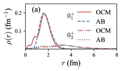
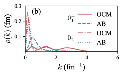
Figure 3: One-body density distributions in (a) coordinate and (b) momentum space for $0_{1}^{+}$ and $0_{2}^{+}$ with the AB and OCM.

Finally, we analyse the component of the ${}^{8}{\rm Be}+\alpha$ configuration in the three-$\alpha$ wave functions to clarify its impact on the geometrical configuration. The spectroscopic amplitude (SA), $y(r)$, is defined by an overlap amplitude between $\Psi_{2\alpha}$ and $\Psi_{3\alpha}$ as a function of the relative distance from the center-of-mass of $\Psi_{2\alpha}$ to the other $\alpha$, where the $\Psi_{2\alpha}$ is the ground-state wave function of ⁸Be with $J^{\pi}=0^{+}$. $\int_{0}^{\infty}[ry(r)]^{2}dr=S$ holds with the spectroscopic factor (SF), $S=\left|\sqrt{\frac{3!}{2!1!}}\braket{\Psi_{2\alpha}Y_{00}(\bm{x}_{2})}{\Psi_{3\alpha}}\right|^{2}$. Note that SF is a subset of $P_{l=0}$ and is listed in parentheses of Tab. 1. The calculated $S$ of $0_{1}^{+}$ for the OCM is small as $P_{l=0}$ is small, while large ${}^{8}{\rm Be}+\alpha$ component is found for the AB. For $0_{2}^{+}$ both models give similar SFs $\approx 0.7$, showing well-developed ${}^{8}\mathrm{Be}+\alpha$ configurations. Figure 4 shows $[ry(r)]^{2}$. For $0_{1}^{+}$, more nodes appear for the OCM in the internal region as expected. Due to the orthogonality condition, the peak is somewhat shifted to outer regions for the OCM. For $0_{2}^{+}$, the positions of these peaks are located at $\approx 5$ fm. Note that the calculated rms distances of ⁸Be are 6.36 and 5.93 fm for the AB and OCM, respectively, which are larger than the respective peak positions of the SA. Reminding that the $S$ value is quite large for $0_{2}^{+}$, this ${}^{8}{\rm Be}+\alpha$ correlation originates the peak structures of the isosceles triangle shape in $0_{2}^{+}$ shown in Fig. 1. We see notable difference between the results of the AB and OCM in the asymptotic regions, reflecting the rms radii obtained by these different models, 3.39 and 4.58 fm for the AB and OCM, respectively. A careful investigation including comparison to available experimental data is necessary to clarify the dominant $\alpha$-cluster configurations in the spectrum of ¹²C.

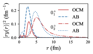
Figure 4: Spectroscopic amplitudes of ${}^{8}\mathrm{Be}+\alpha$ for $0_{1}^{+}$ and $0_{2}^{+}$ with the OCM and AB.

3 Summary and future perspectives

To extract geometric configurations of three-$\alpha$ particles in the ground and first excited $0^{+}$ states of ¹²C, we have performed precise three-$\alpha$ calculations using two types of potential models, the orthogonality condition model (OCM) and the shallow potential model (AB), which produce different internal structure of the wave functions. Analyzing the wave functions in detail, we show that the ${}^{8}{\rm Be}+\alpha$ configuration plays a crucial role to form isosceles triangle shape in the first excited $0^{+}$ state. The notable differences in the wave functions with the OCM and AB can possibly be distinguished by physical observables. A comparison with experiment, e.g., the decay properties and electromagnetic transitions including other $J^{\pi}$ state is necessary to verify these adopted models for establishing the three-$\alpha$ configurations in the spectrum of ¹²C.

References

- (1) F. Hoyle, Astrophys. J. Suppl. 1, 121 (1954)
- (2) A. Tohsaki, H. Horiuchi, P. Schuck, G. Röpke, Phys. Rev. Lett. 87, 192501 (2001)
- (3) L. Fortunato, Phys. Rev. C 99, 031302(R) (2019)
- (4) A. Vitturi, J. Casal, L. Fortunato, E. G. Lanza, Phys. Rev. C 101, 014315 (2020)
- (5) S. Saito, Prog. Theor. Phys. 40 893 (1968); 41 705 (1969); Suppl. 62, 11 (1977)
- (6) S. Ali, A. R. Bodmer, Nucl. Phys. 80, 99-112 (1966)
- (7) E.C.Pinilla,D.Baye,P.Descouvemont,W.Horiuchi,Y.Suzuki, Nucl. Phys. A 865, 43 (2011)
- (8) T. Arai, W. Horiuchi, D. Baye, Nucl. Phys. A 977, 82 (2018)
- (9) C. Kurokawa, K. Katō, Phys. Rev. C 71, 021301 (2005)
- (10) C. Kurokawa, K. Katō, Nucl. Phys. A 792, 87-101 (2007)
- (11) V. I. Kukulin, V. N. Pomenertsev, Ann. Phys. (N. Y.) 111, 330 (1978)
- (12) D. V. Fedorov, A. S. Jensen, Phys. Lett. B 389, 631 (1996)
- (13) S. Ishikawa, Phys. Rev. C 87, 055804 (2013)
- (14) S. Ishikawa, Phys. Rev. C 90, 061604(R) (2014)
- (15) N. B. Nguyen, F. M. Nunes, I. J. Thompson, Phys. Rev. C 87, 054615 (2013)
- (16) K. Varga, Y. Suzuki, Phys. Rev. C 52, 2885 (1995)
- (17) Y. Suzuki, K. Varga, Stochastic Variational Approach to Quantum-Mechanical Few-Body Problems, Lecture Notes in Physics, Vol. m54 (Springer, Berlin, 1998)
- (18) Lai Hnin Phyu, H. Moriya, W. Horiuchi, K. Iida, K. Noda, M. T. Yamashita, Prog. Theor. Exp. Phys. 2020, 093D01 (2020)
- (19) Y. Suzuki, W. Horiuchi, M. Orabi, K. Arai, Few-Body Syst. 42, 33 (2008)
- (20) J. Mitroy, S. Bubin, W. Horiuchi, Y. Suzuki, L. Adamowicz, W. Cencek, K. Szalewicz, J. Komasa, D. Blume, K. Varga, Rev. Mod. Phys. 85, 693-749 (2013)
- (21) Y. Suzuki, W. Horiuchi, Emergent Phenomena in Atomic Nuclei from Large-scale Modeling: A Symmetry-Guided Perspective (World Scientific, Singapore, 2017), Chap. 7, pp. 199-227
- (22) S. Ohtsubo, Y. Fukushima, M. Kamimura, E. Hiyama, Prog. Theor. Exp. Phys. 2013, 073D02 (2013)
- (23) Y. Suzuki, K. Arai, Y. Ogawa, K. Varga, Phys. Rev. C 54, 2073 (1996)
- (24) W. Horiuchi, Y. Suzuki, Phys. Rev. C 90, 034001 (2014)
- (25) Yu. F. Smirnov, I.T. Obukhovsky, Yu. M. Tchuvil’sky, V. G. Neudatchin, Nucl. Phys. A 235 289 (1974)
- (26) T. Yamada, P. Schuck, Eur. Phys.J. A 26, 185-199 (2005)
- (27) W. Horiuchi, Y. Suzuki, Phys. Rev. C 89, 011304(R) (2014)
- (28) T. Neff, J. Phys. Conf. Ser. 403, 012028 (2012)
- (29) T. Yamada, Y. Funaki, H. Horiuchi, G. Röpke, P, Schuck, A. Tohsaki, in Lecture Notes Physics Cluster Nuclei, edited by C. Beck (Springer, Berlin, Heidelberg, 2012), Vol. 2, Chap. 5, pp. 229-298