Multi-Spectrally Constrained Transceiver Design against Signal-Dependent Interference
Abstract
This paper focuses on the joint synthesis of constant envelope transmit signal and receive filter aimed at optimizing radar performance in signal-dependent interference and spectrally contested-congested environments. To ensure the desired Quality of Service (QoS) at each communication system, a precise control of the interference energy injected by the radar in each licensed/shared bandwidth is imposed. Besides, along with an upper bound to the maximum transmitted energy, constant envelope (with either arbitrary or discrete phases) and similarity constraints are forced to ensure compatibility with amplifiers operating in saturation regime and bestow relevant waveform features, respectively. To handle the resulting NP-hard design problems, new iterative procedures (with ensured convergence properties) are devised to account for continuous and discrete phase constraints, capitalizing on the Coordinate Descent (CD) framework. Two heuristic procedures are also proposed to perform valuable initializations. Numerical results are provided to assess the effectiveness of the conceived algorithms in comparison with the existing methods.
Index Terms:
Multiple Spectral Compatibility Constraints, Signal-Dependent Interference, Continuous and Discrete Phase-Only Waveform Design, Coordinate Descent (CD) Method.I Introduction
Spectral coexistence among radar and telecommunication systems has drawn flourishing attention due to the conflict between limited Radio Frequency (RF) spectrum resource and the increasing demand of spectrum access [1, 2, 3, 4, 5]. Waveform diversity and cognitive radar are key candidates to alleviate this problem via on the fly adaptation of the transmitted waveforms to actual spectrally contested and congested environments[6, 7, 8, 9, 10, 11, 12, 13, 14, 15]. In this respect, a plethora of papers in the open literature have dealt with the problem of designing cognitive radar signals with a suitable frequency allocation so as to induce acceptable interference levels on the frequency-overlaid systems, while improving radar performance in terms of low range-Doppler sidelobes, detection, and tracking abilities[16, 17, 18, 19, 20, 21, 22, 23, 24, 25].
In [26], a technique to synthesize constant envelope signals sharing a low Integrated Sidelobe Level (ISL) and a sparse spectral allocation is developed, considering as objective function a weighted sum between an ISL-oriented contribution and a term accounting for the waveform energy over the licensed bandwidths. The mentioned approach is generalized to provide a control on the waveform ambiguity function features in [27]. Some interesting algorithms to devise radar waveforms under spectral compatibility requirements, are also proposed in [28, 29, 30], where different performance criteria, like amplitude dynamic range, Peak Sidelobe Level (PSL), spectral shape features, and distance from a reference code, are considered at the signal design process. [31] introduces the spectral shaping (SHAPE) method to synthesize constant-modulus waveforms aimed at fitting an arbitrary desired spectrum magnitude, whereas in [32] and [33] the Spectral Level Ratio (SLR) is adopted as performance metric assuming, respectively, constant envelope and PAR constraints. In [34, 35, 1, 36], the maximization of Signal to Interference plus Noise Ratio (SINR) is accomplished in the presence of signal-independent disturbance while controlling the total interference energy on the common band and some desirable features of the transmitted waveform. This framework is extended to incorporate multiple spectral compatibility constraints in[37]. Along this line, to comply with the current amplifier technology, extensions to address optimized synthesis of constant envelop waveforms with the continuous phase[38] and the finite alphabet[39], are developed. However, the studies in [34, 35, 1, 36, 37, 38, 39] do not account for signal-dependent interference at the design stage, namely they implicitly assume that the radar is pointing toward the sky (with very low antenna sidelobes) or the target range is far enough that ground clutter is substantially absent. Some attempts to design radar transceivers capable of lifting up detection performance in a highly reverberating environment as well as ensuring spectral compatibility have been pursued in the open literature. For instance, [40] and [41] optimize the SINR (in the presence of signal-dependent disturbance) over the transmit signal and receive structure, while controlling the total amount of interference energy injected on the shared frequency bands. Still forcing a constraint on the global spectral interference, [42, 43, 44] propose waveform design procedures in the context of Multiple-Input Multiple-Output (MIMO) radar systems operating in highly reverberating environments. Besides, [42] also extends the developed framework considering multiple spectral constraints but just an energy constraint is forced on each transmitted signal. Nevertheless, the design of constant envelope signals ensuring the appropriate Quality of Service (QoS) to each licensed system still remains an open issue.
Aimed at filling this gap, in this paper, a new radar transceiver design strategy (with phase-only probing signals) is proposed aimed at optimizing surveillance system performance (via SINR maximization in signal-dependent interference) while fully guaranteeing coexistence with the surrounding RF emitters. Specifically, unlike most of the previous works111Preliminary results of continuous phase codes are shown in [45] without technical details., a local control on the interference energy radiated by the constant envelope signal on each reserved frequency bandwidth is performed, so as to enable joint radar and communication activities. Moreover, to comply with the current amplifiers technology (operating in saturation regime) constant envelope waveforms are considered, with either arbitrary or discrete phases. Besides, to fulfill basic radar requirements, in addition to an upper bound to the maximum radiated energy, a similarity constraint is enforced to bestow relevant waveform hallmarks, i.e., a well-shaped ambiguity function. To handle the resulting NP-hard optimization problems, a suitable re-parameterization of the radar code vector is performed; hence, leveraging the Coordinate Descent (CD) method [46], iterative algorithms (monotonically improving the SINR) are proposed (for both continuous and discrete phase constraints), where either a specific entry of the transmitter parameter vector or the receive filter is optimized at a time while keeping fixed the other variables. Specifically, a global optimal solution of each, possibly non-convex, optimization problem (involved in the two developed procedures) is derived in closed form through the evaluation of elementary functions. Regardless of the phase cardinality, the computational complexity is linear with respect to the number of iterations, cubic with reference to the code length, and less than quadratic with respect to the number of spectral constraints. Finally, two heuristic approaches, accounting for spectral compatibility requirements via a penalty term in the objective function, are proposed to initialize the procedures via ad-hoc starting solutions. To shed light on the capability of the devised algorithms to counter signal-dependent interference and ensure coexistence with the overlaid RF emitters, some case studies are provided at the analysis stage. Moreover, appropriate comparisons with some counterparts available in the open literatures are presented to prove the effectiveness of the new proposed strategies.
The paper is organized as follows. In Section II, the system model is introduced, followed by the definition and description of the key performance metrics as well as constraints involved into the formulation of radar transceiver design problems under investigation. In Section III, innovative solution methods are developed to handle the NP-hard optimization problems at hand. Section V presents some numerical results to assess the performance. Finally, in Section VI, concluding remarks and some possible future research avenues are provided.
-
•
Bold letters, e.g., (lower case), and (upper case) denote vector and matrix, respectively.
-
•
, , and indicate the transpose, the conjugate, and the conjugate transpose operators, respectively.
-
•
, , are the sets of -dimensional vectors of real and complex numbers, and of -dimensional Hermitian matrices, respectively.
-
•
For any , and represent the Euclidean and -infinity norm, respectively.
-
•
and represent the -dimensional identity matrix and the matrix with zero entries.
-
•
is the -dimensional vector with all entries equal to 1.
-
•
is a vector whose -th entry is and other elements are .
-
•
Letter represents the imaginary unit (i.e., ).
-
•
, and mean the real, imaginary part, and modulus of a complex number, respectively.
-
•
represents the argument of the complex number .
-
•
indicates the diagonal matrix formed by the entries of .
-
•
indicates the diagonal matrix whose -th diagonal element is
-
•
is the shift matrix with if , else , .
-
•
is the largest eigenvalue of .
-
•
The statistical expectation is indicated as .
-
•
and () provide the greatest integer not larger than and the lowest integer not smaller than , respectively.
-
•
denotes the integer closest to . If the decimal part of is 0.5, , else .
-
•
is the Hadamard element-wise product.
-
•
is the optimal value of the optimization Problem .
-
•
denote the derivative of with respect to .
II Problem Formulation
This section is focused on the introduction of the system model accounting for a highly reverberating environment, as well as on the formulation of the constrained optimization problem to jointly design radar transmitter and receiver.
II-A System Model
Let be the transmitted fast-time radar code with being the number of coded sub-pulses. The observations from the range-azimuth cell under test (CUT) are collected in the vector , which can be expressed as [40]
| (1) |
where
-
•
accounts for the response of the prospective target within the CUT.
-
•
is the signal-dependent interference produced by the range cells adjacent to the CUT, namely
(2) with the scattering coefficient associated with the -th range patch. Specifically, are modeled as independent complex, zero-mean, circularly symmetric, random variables with . As a result, the covariance matrix of can be cast as
(3) -
•
denotes the signal-independent interference that comprises thermal noise and other disturbances from interfering emitters. It is modeled as a zero-mean, complex, circularly symmetric, random vector with covariance .
II-B Transmit Code Constraints
In this subsection, some constraints on the transmitted signal are introduced to fulfill the appropriate radar requirements [47, 48].
II-B1 Multi-Spectral Constraints
To assure spectral compatibility with the surrounding licensed emitters, the radar has to control the spectral shape of the probing waveform to manage the amount of interfering energy injected on the shared frequency bandwidths. In this respect, let us denote by the number of licensed emitters while and indicate the lower and upper normalized frequencies (with respect to the underlying radar sampling frequency) for the -th system, respectively. Now, denoting by the Energy Spectral Density (ESD) of the fast-time code , the energy transmitted by the radar within the -th licensed bandwidth (also denoted by stopband) can be expressed as
| (4) |
where for ,
To enable joint radar and communication activities, it is thus demanded that the radar transmitted waveform complies with the constraints
| (5) |
where , , accounts for the acceptable level of disturbance on the -th bandwidth and is tied up to the QoS required by the -th communication system.
II-B2 Constant Envelope and Energy Constraints
To assure compatibility with the amplifier technology and comply with the radar power budget, constant envelope and energy constraints are forced on the sought waveform, which is tantamount to forcing
| (6) | |||||
| (7) |
II-B3 Finite Alphabet Constraint
As a limited number of bits are available in digital waveform generators, the finite alphabet constraint is possibly forced, requiring , where denotes the discrete set of equi-spaced phases.
II-B4 Similarity Constraint
To bestow some desirable attributes (e.g., Doppler tolerance, ISL, PSL and etc.) to the radar probing signal, a similarity constraint is imposed on the transmitted code, i.e.,
| (8) |
where rules the size of the trust hypervolume, and is a specific constant modulus reference code with .
II-C Transceiver Design Problem Formulation
A transceiver design approach aimed at optimizing target detectability under the probing code requirements of Subsection II-B is now formalized. To this end, supposing the received signal filtered via , the SINR at the output of the filter, i.e.,
| (9) |
is considered as the design metric.
Hence, according to the code limitations introduced in Subsection II-B, the joint transmit-receive pair design assuming either continuous phase or finite alphabet phase codes, respectively, can be formulated as the following non-convex and in general NP-hard optimization problems222If and are statistically independent and Gaussian distributed, the SINR optimization is tantamount to maximizing the detection probability.
| (10) |
and
| (11) |
with and .
III Code and Filter Synthesis
In this section, an iterative design procedure is developed to get optimized transmit-receive pairs leveraging the CD paradigm [46]. By invoking elementary function, each nonconvex optimization subproblem is solved in closed form, and the monotonic improvement of the SINR is ensured along the iterations. As first step toward this goal, let us re-parameterize the optimization vector as
| (12) |
where , with , and () account for code phases and the signal amplitude level, respectively. As a result, the similarity constraint is tantamount to . Hence, denoting by , for any
-
•
for the continuous case[38];
- •
Additionally, in the transformed domain, the spectral constraints can be cast as
| (13) |
where . Finally, the objective function in (11) can be expressed as
| (14) |
with
To proceed further, let us introduce the optimization vector and denote by the function (14) evaluated at . Consequently, Problems and can be equivalently cast as
| (15) |
where is either an integer number or and specifies the code alphabet size.
The provided reformulation in (15) paves the way for an effective CD-based optimization process, where the design variables of the vector are partitioned into blocks given by , with corresponding to the receive filter. Hence, at the -th step, , of the -th iteration, the -th block is optimized with the other blocks fixed at their previous optimized value. Now, denoting by , it follows that
The above inequalities entail that the objective function values monotonically increase along with the iterations. Thus, being upper bounded by with the variance of thermal noise, converges to a finite value. In the following, the procedures devised to optimize the -th block, , at the -th iteration are developed. This represents the main technical achievement of this paper from an optimization theory standpoint.
III-A Code Phase Optimization
Assuming , the block to optimize is , with the other blocks set to their previous optimized values, i.e., , . Hence, as shown in Appendix -A, the problem to solve is
| (16) |
where
The feasible set333 To avoid unnecessary complications, is assumed. of Problem and the monotonicity properties of are analyzed in Appendix -B with specification of global maximizer and minimizer and , respectively. In particular, it is shown that can be expressed as
| (17) |
where (see Appendix -B for details)
-
•
is the number of disjoint intervals that compose with , , depending on the specific instance of Problem and such that .
-
•
is the number of disjoint discrete sets that form with , and .
The following proposition paves the way to the solution of the non-convex optimization problem .
Proposition III.1.
An optimal solution to can be evaluated in closed form via the computation of elementary function as follows:
-
•
if the unconstrained global optimal solution is feasible, i.e., , the optimal solution is ;
-
•
otherwise, if , the optimal solution belongs to , i.e.,
(18) -
•
else, denoting by , the optimal solution is
(19)
Proof.
See Appendix -C. ∎
According to Proposition III.1, as long as does not belong to one of the closed and bounded intervals , the global optimal solution is one of the intervals extremes. As a consequence, embedding to an appropriate union of closed intervals the following corollary holds true.
Corollary III.1.
An optimal solution to can be derived as follows:
-
•
if there exists an index satisfying , then
(20) where
(21) -
•
otherwise, if ,
(22) -
•
else,
(23) where .
Proof.
See Appendix -D. ∎
Hence, starting from a feasible solution , the solution to for different values of the objective parameters can be easily accomplished following the line of Algorithm 1.
Input: , , , , , , , , , ;
Output: ;
-
1.
Compute the feasible set as given in (17);
-
2.
If , ,
-
3.
Elseif, ,
-
4.
Else,
where ;
-
5.
Output .
III-B Code Amplitude Optimization
Focusing on , w.r.t. reduces to the following problem,
where , and . The first-order derivative of the objective function satisfies
Hence, the objective function monotonically increases over , and the optimal solution is just the highest feasible value, given by
| (24) |
III-C Receive Filter Optimization
With reference to the -th variable block, the optimization variable is the receive filter. The update of the receive filter, i.e., , is tantamount to solving
| (25) |
where is the updated transmit signal at the -th iteration. The optimal solution [40] is
| (26) |
Remark III.1.
Supposing which is positive definite, the solution to the linear equations can be derived via the Conjugate Gradient Method (CGM) [49].
III-D Optimization Process and Computational Complexity
Starting from a feasible solution , the overall iterative design procedure is summarized in Algorithm 2. Note that in place of the standard cyclic updating rule, the Maximum Block Improvement (MBI) strategy [50] can be used, too. As to the computational complexity of Algorithm 2, it is linear with the number of iterations. In each iteration, it mainly includes the computation of the code phases (step 3), the code amplitude (step 4), and the receive filter (step 5), whose complexities are now discussed.
Step 3 includes the solution of , and the main actions to perform at each are:
-
1.
evaluation of the problem parameters;
-
2.
calculation of ;
-
3.
determination of the optimal phase.
As to item 1, the parameters to compute are , , , , , and , , . Leveraging smart recursive schemes based on suitable support variables, it follows that for a complete algorithm iteration the computational complexity of and is whereas that of and is . With reference to , it requires multiplications for any and . Furthermore, following the same line of reasoning as in [38], for any , , can be updated by canceling out the items related to the variable from , and adding those involving , with a complexity of ; similar considerations hold true with respect to . Hence, the overall computational complexity of item 1 at each algorithm iteration is . As to item 2, note that the determination of can be performed with a computational complexity of for any leveraging the results of [38]. Besides, according to Appendix -B, can be obtained resorting to appropriate quantizations of and , with an extra computational complexity of . With reference to item 3, the unconstrained optimal solution , for any , can be evaluated via elementary functions using , , , and with a computational burden of , while the optimal solution to the Problem can be accomplished with a complexity at most of positioning within , in the correct sorted location.
With reference to the complexities of step 4 and 5, the former (mainly related to the efficient computation of ) is , the latter requires operations, with the most demanding task given by the evaluation of ; in particular, according to the Remark III.1, (26) can be efficiently computed by CGM with a complexity of where is the number of iterations. Therefore, the overall computational complexity of steps 3, 4 and 5 is .
Input: Reference code , phase cardinality , initial feasible code (resp. ), , minimum required improvement , , , , and , ;
Output: Optimized solution ;
IV Heuristic Methods for Algorithm Initialization
The solution provided by Algorithm 2 depends on the initial feasible sequence . Thus, the development of a heuristic procedure ensuring high quality starting points is valuable. To this end, an ad-hoc transceiver synthesis strategy is proposed, accounting for the spectral constraints via a penalty term in the objective function. Specifically, the following design problem is considered
| (27) |
with
| (28) |
where is a weighting factor ruling the relative importance between the two objectives444 can be interpreted as a weight which scalarizes the multi-objective optimization problem involving the SINR and the opposite total interference energy on the licensed bands as figure of merits., and . Thus, denoting by an optimized solution to (27), the initial feasible code to Algorithm 2 can be constructed as
| (29) |
Note that Problem (27) is in general NP-hard. As a first step to handle this synthesis, let us re-parameterize the transmit signal as ; hence, Problem (27) boils down to
| (30) |
where is the new optimization vector (with and ), (with ) is the feasible set of , and , namely it denotes the objective in (28) evaluated at .
To solve Problem (30), the optimization framework in [51] and [50] is used. The main idea of this solution strategy is to partition the variables of the optimization vector into decoupled blocks555It is assumed that , with the feasible set of -th block of variables, ., i.e., avoiding useless complications, , where with , and update one block at a time666Either an alternating or an MBI strategy can be considered.. The procedure is reported in Algorithm 3 assuming an alternating optimization rule and no approximations to the feasible set. Therein, focusing on the optimization of the -th variables block (), , for and , represents the surrogate function to maximize, which shares the following properties [51, 50]:
-
(P1)
is continuous with respect to and ;
-
(P2)
for and ;
-
(P3)
.
According to [50, Proposition 2] and [51, Theorem 1], Algorithm 3 ensures a monotonic improvement of the objective, and, under some mild technical conditions, the convergence to a stationary point for any limit point of the generated sequence of the feasible solutions.
Input: A feasible starting point
, .
Output: Optimized solution to Problem (27);
-
1.
Set ;
-
2.
Repeat;
-
3.
For ,
-
4.
-
5.
;
-
6.
;
-
7.
End
-
8.
Until convergence;
-
9.
Output .
In the following subsections, two solution techniques leveraging the optimization framework in Algorithm 3 are proposed to tackle (30). The former considers as optimization blocks and . The latter assumes optimization blocks, given by .
IV-A Heuristic Initialization Via Alternating Optimization with MM (HIVAM)
The optimization variable is partitioned into two blocks, i.e., , . At -th step, the surrogate functions involved in the optimization of and are given, respectively, by (see Appendix E in the supplemental material for details)
| (31) |
| (32) |
where . Moreover, , and .
As a consequence, at -th step,
-
1.
the first block is updated (the interested reader may refer to Appendix -E for technical details) as
(33) where
-
•
if ,
-
•
if ,
with .
-
•
-
2.
the second block is updated as
(34)
IV-B Heuristic Initialization via Alternating Optimization with CD (HIVAC)
The optimization variable is partitioned into blocks, i.e., , . The surrogate functions are obtained restricting the objective function to , namely,
Otherwise stated,
| (35) |
| (36) |
with , , , , , reported in Appendix -F. Besides, , and .
As a consequence, at -th step,
- 1.
-
2.
the -th block is optimized as
(38) where .
V Performance Analysis
This section is devoted to the performance assessment of Algorithm 2 in terms of achievable target detectability, spectral shape of the synthesized transmit waveform and receive filter, and cross-correlation features. In this respect, a radar with a two-sided bandwidth of 2 MHz and a pulse length of 100 s (leading to ) is considered. As to the reference code , a unitary energy Linear Frequency Modulated (LFM) pulse of 100 s and a chirp rate Hz/s is employed for the continuous phase. The -quantized version of the above chirp is instead considered for the finite alphabet case, with cardinality 777Unless otherwise stated, three different initializations are adopted for Algorithm 2 (with ): HIVAM (with ), HIVAC (with ), and the third corresponds to the optimized code at the previous value. The one providing the highest among the three synthesized sequences is picked up. As to the hyperparameter involved in the initialization process, it has been empirically shown that and provide satisfactory performance in all the scenarios and can be used in HIVAM and HIVAC, respectively. .
The covariance matrix of signal-independent interference is
| (39) |
where dB is the thermal noise level; dB, , accounts for the energy of the -th licensed emitter operating over the normalized frequency interval with the related bandwidth extent (, ); is the normalized covariance matrix of the -th non-licensed active source, whose normalized carrier frequency, bandwidth, and power are denoted by , and , respectively ( dB, , dB, , ,). For the signal-dependent interference, dB, , is assumed. Besides, the radar probing waveform is required to fulfill the spectral compatibility constraints corresponding to dB and dB, respectively.
V-A Target Detectability Assessment
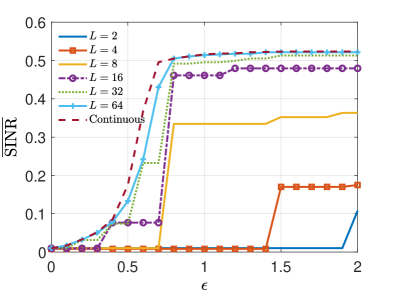
Fig. 1 depicts the normalized SINR achieved by the proposed transceiver design strategy versus for continuous and discrete phase codes (). As expected, a larger similarity parameter leads to a higher value regardless of phase cardinality being available more degrees of freedom (DOF) at the design stage. Besides, the finer the phase discretization, the better the performance, with curves of the synthesized discrete phase codes closer and closer to that of the continuous phase benchmark. Finally, it is worth pointing out that the designed sequence coincides with a scaled version of reference code, with an energy modulation implemented to comply with the forced spectral constraints if (for the continuous phase) or (for the finite alphabet). For instance, for the binary case as long as , and thus a performance improvement just appears at . Consequently, the similarity parameter should be carefully selected to balance the detection performance and waveform characteristics.
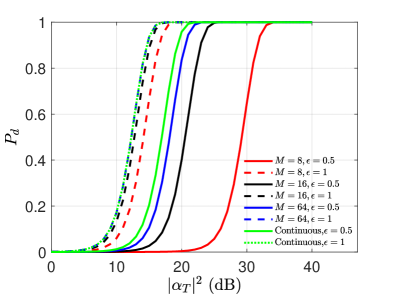
Now, assuming and statistically independent and Gaussian distributed as well as a Swerling 0 target, the probability of detection () versus , as function of and the phase discretization step, is shown in Fig. 2. Therein, the same environmental characterization as in Fig. 1 is considered and the false alarm probability () is set to . As expected, increasing of similarity parameter, the cardinality of the code alphabet, and provide improvements.
To the best of the Authors’ knowledge, the waveform design methods currently available in the open literature are not able to solve Problem in its general form. Aimed at providing a complete assessment of Algorithm 2, in Subsection V-C some specific instances of Problem are analyzed, reporting the comparison of our new method with other suitable approaches already devised in the open literature [52, 42].
V-B Transceiver Characteristics
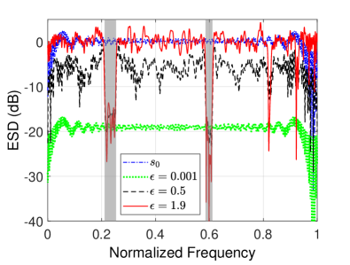
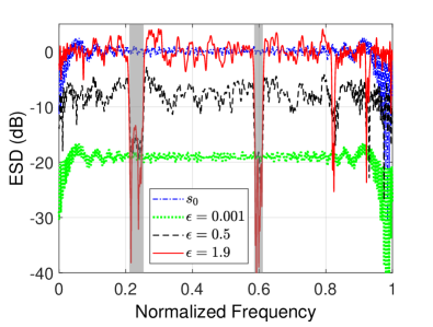
In Fig. 3, the spectral behavior of the signals synthesized through Algorithm 2 (in terms of ESD versus the normalized frequency) is provided as function of the similarity parameter. Specifically, Fig. 3 (a) refers to the continuous phase design, whereas Fig. 3 (b) is related to . Therein, the stopbands are shaded in light gray. The curves highlight the capability of the devised techniques to suitably control the amount of interference energy produced over the shared frequency bandwidths, as required by the imposed spectral compatibility constraints. Furthermore, inspection of the figures reveals that, regardless of the code cardinality, the ESD curve corresponding to almost coincides with a scaled version of the considered reference code, as a result of the energy modulation performed to ensure cohabitation, along with the similarity requirement. Finally, an improvement in the “useful” energy distribution is achieved as increases, with deeper and deeper spectral notches in correspondence of the jammed frequencies, especially for the continuous alphabet code.
To shed light on the capabilities of the devised transceiver to mitigate signal-dependent disturbance, the PSL and ISL of the Cross-Correlation Function (CCF) normalized to between the transmit waveform and the receive filter versus the iteration index, are reported in Table II for the continuous phase and , assuming and HIVAM as the initialization method. The results show that lower and lower PSL and ISL values are achieved as the iteration step grows up for both continuous and discrete phase codes. Otherwise stated, the devised strategy is able to iteratively improve the rejection of the signal-dependent interference.
|
||||||||||||
| 0 | 2 | 4 | 8 | 15 | ||||||||
| PSL(dB) | -18.25 | -19.63 | -20.39 | -21.19 | -21.22 | |||||||
| ISL(dB) | -6.95 | -7.78 | -8.12 | -8.47 | -8.52 | |||||||
|
||||||||||||
| 0 | 2 | 5 | 10 | 20 | ||||||||
| PSL(dB) | -18.39 | -20.24 | -20.96 | -21.08 | -21.34 | |||||||
| ISL(dB) | -6.49 | -7.89 | -8.18 | -8.32 | -8.39 | |||||||
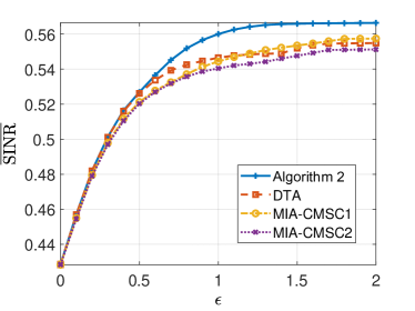
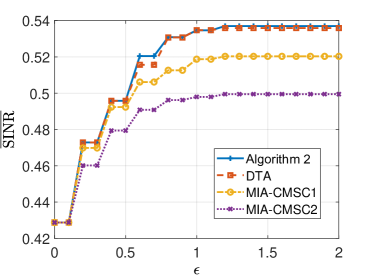
V-C Comparison with Available Algorithms
If spectral coexistence requirements are not considered, the resulting problem can be solved by Dinkelbach-Type Algorithm (DTA) [52] and Majorized Iterative Algorithm with the Constant Modulus and Similarity Constraint (MIA-CMSC) [42], which can be further distinguished into MIA-CMSC1 and MIA-CMSC2 depending on different majorization methods888The parameters specified in [52] and [42] are used to implement these algorithms; specifically, and for DTA and for MIA-CMSC1 and MIA-CMSC2.. Figs. 4(a)-(b) depict the achieved by Algorithm 2, DTA, MIA-CMSC1, and MIA-CMSC2 assuming at the design stage a continuous phase and , respectively999For all the algorithms at each both the reference sequence and the code optimized at the previous are adopted as the initializations. The one providing the highest between the two synthesized sequences is picked up. Although DTA and MIA-CMSC are not provided in [52] and [42] with reference to discrete phase codes, their extension to encompass also this design constraint is straightforward.. Looking over the figures unveils that the proposed CD framework outperforms the counterparts. The superior performance with respect to DTA can be attributed to the slight phase-search sub-optimality of the DTA, which is intrinsic in the Dinkelbach iterative method. Instead, the performance loss incurred by the MIA-CMSC methods reasonably results from the approximation of the objective function performed in the procedure. Finally, in the design of discrete phase codes MIA-CMSC procedures experience a higher performance gap with respect to Algorithm 2 than that observed for the continuous phase instance.
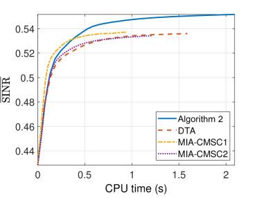
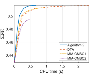
To assess the convergence property and computational complexity of the different methods, Figs. 5(a)-(b) depict the versus CPU time with for the continuous phase and , respectively. The reference code is used for this case study to initialize all the algorithms. As expected, the objective function of all the methods monotonically increases. Inspection of the curves shows that Algorithm 2 is substantially capable of obtaining larger values than the counterparts for any given time budgets, which provides a practical proof of the CD framework efficiency. Specifically, Algorithm 2 outperforms the counterparts, but for the continuous phase code synthesis and up to 0.38s where MIA-CMSC1 is better.
To proceed further, let us observe that, neglecting the constant envelope as well as the similarity requirements, with can be solved via Majorized Iterative Algorithm with the Spectrum Compatibility Constraint for Local design (MIA-SCCL)[42], as well as a variant of the algorithm in [40], denoted as SemiDefinite Programming-based Design (SDPD)101010The parameters specified in [42] and [40] are used for implementing these algorithms; specifically, and for MIA-SCCL and for SDPD.. The , the computational time, and the PAR [27] of the sequences synthesized via SDPD, MIA-SCCL and Algorithm 2 are summarized in the Table III. The sequence devised via HIVAC is adopted as the initialization for all the algorithms, which costs 1.8724s for computation. The proposed CD algorithm is capable of devising the radar transceiver with a shorter running time than the counterparts. However, as expected, it experiences a loss with respect to SDPD and MIA-SCCL. Indeed, SDPD and MIA-SCCL may capitalize on code amplitude variation to boost the radar performance, at the price of larger PAR values, which in turn demand for more sophisticated amplifiers.
| Algorithm | Time (s) | PAR | |
| SDPD | 0.6088 | 855.4809 | 2.4520 |
| MIA-SCCL | 0.6004 | 6.6539 | 3.3589 |
| CD | 0.5120 | 1.7256 | 1 |
VI Conclusion
The synthesis of radar transceivers in signal-dependent interference and spectrally contested-congested environments has been addressed in this paper. Specifically, assuming constant modulus signals with either continuous or finite alphabet phases, the design has aimed at maximizing the SINR at the output of the receive filter while ensuring cohabitation with surrounding RF systems via multiple spectral constraints. Furthermore, a similarity constraint has been forced on the probing signal to bestow attractive waveform characteristics. Hence, resorting to the CD framework, iterative procedures (with ensured convergence properties) have been conceived to synthesize optimized radar waveforms and receive filters. Each step requires the solution of a possible non-convex optimization problem whose global optimal point is obtained in closed-form, regardless of the phase codes cardinality. Remarkably, the overall computational complexity of the proposed algorithms is polynomial with respect to both the code length and the number of licensed emitters.
At the analysis stage the performance of the synthesized transceiver pair has been assessed in terms of different metrics, i.e., SINR as well as detection probability, spectral shape, and CCF features. The results have clearly shown that the proposed framework is capable of mitigating diverse interfering scenarios, while ensuring cohabitation with overlaid licensed systems. Besides, some comparisons with counterparts available in the open literature have been provided, showing interesting performance gains, in terms of achieved SINR and/or computational time.
Future research tracks might concern the extension of this framework to MIMO radar systems where spatial diversity may induce other degrees of freedom which can be optimized to improve the performance of the overall method.
ACKNOWLEDGMENT
This research activity has been conducted during the visit of Jing Yang at the University of Napoli “Federico II" DIETI under the local supervision of Prof. A. Aubry and Prof. A. De Maio. The Authors would like to thank Dr. Linlong Wu, Prof. Prabhu Babu, and Prof. Daniel P. Palomar for providing the MATLAB code for MIA.
-A Derivation of Problem (16)
Before proceeding further, let us introduce the following lemma.
Lemma 1.
For any known matrix , with can be recast as a function of a specific entry , i.e.,
| (40) |
where , and .
According to Lemma 1 and exploiting as well as , w.r.t. can be expressed as
| (41) |
where
-
•
,
-
•
,
-
•
,
-
•
,
with .
Similarly, the spectral constraints can be transformed as
| (42) |
where , . As a result, being , the inequalities in (42) are tantamount to , where .
-B Monotonicity Study of and Evaluation of
Before proceeding further, let us observe that both the characterization of the objective function monotonicities and the feasible set derivation can be performed by means of a change of variable, that defines a one-to-one monotonically increasing mapping. To this end, let us consider . In the transformed domain, the objective function of Problem (16) can be rewritten as
| (43) |
where
| (44) |
Similarly, can be cast as
| (45) |
where
| (46) | |||||
Let us first characterize the behavior of the objective function . To this end, note that , which implies that either and , or and . As to the first-order derivation of , it is given by
| (47) |
where , and . According to Lemma 2 (reported below), if , admits two stationary points. In particular, exhibits the following behavior:
-
•
if , it follows that
-
–
if , it follows that , implying that is a constant function;
-
–
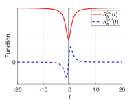
if (see Fig. 6 (a) for a notional example), is strictly decreasing over , and strictly increasing over . Thus, the minimum point is , and the finite supremum is achieved at .
-
–
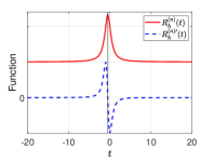
if (see Fig. 6 (b) for a notional example), is strictly increasing over , and strictly decreasing over . Thus, the maximum point is , and the finite infimum is achieved at ;
-
–
-
•
if , the roots of (47) are ruled by the discriminant , which are given by , ;
As already pointed out, since is mapped to by a strictly increasing function, the monotonicities of can be directly derived starting from those of . For instance, supposing , is strictly increasing over with , then decreasing over with , and increasing over . As a result, the maximum and minimum points , of the objective function are111111Note that if and , is a constant function, thus the maximum and minimum points are assigned as and .
and
Let us now focus on the feasible set evaluation, which is not empty being a feasible solution to . Precisely, omitting the dependence on and for notational simplicity and considering the continuous phase case, the feasible set in the transformed domain is given by
| (48) |
where
| (49) |
and .
As shown in [38], can be cast as
| (50) |
with , whose specific values depend on , , , and , and can be derived relying on De Morgan law and “union-find" algorithm. As a consequence, the feasible set of Problem can be expressed as
| (51) |
where , .
As to the discrete phase case, let us observe that
| (52) |
Denoting by with
| (53) |
can be recast as
| (54) |
with the condition ensuring that is not empty. Now actually, denoting by the number of sets involved in the union operation of (54) (i.e., the number of the actual disjoint closed sets), there exists an increasing mapping : , such that . Hence, denoting by , can be rewritten as
| (55) |
Lemma 2.
If , Eq. (47) admits two roots.
Proof.
Let us proceed by contradiction and assume . If , which entails that , two situations may occur:
-
1.
, which implies that ; thus, is a non-decreasing function and in particular, .
-
2.
, leading to ; hence, is a non increasing function implying that .
Based on (43), , that according to the aforementioned monotonicities leads to , . Hence, , , namely, , which contradicts the assumption . ∎
-C Proof of Proposition III.1
Proof.
To solve Problem , it is convenient to distinguish among different situations according to the specific instances of and . Evidently, if is feasible, i.e., , of course .
Let us now suppose that is outside of ,
-
•
if , the optimal solution depends on the actual monotonicities of the objective function:
-
–
if and , or , monotonically decreases over , which implies ;
-
–
if , monotonically decreases over , and then strictly increases over , then ;
-
–
-
•
if , a situation dual to occurs:
-
–
if and , or , monotonically increases over , which implies ;
-
–
if , monotonically decreases over , and then increases over , thus .
-
–
-
•
if , two situations may occur:
-
–
if and , is a constant for all , thus ;
-
–
if and , monotonically decreases over , and then increases over , then ;
-
–
Hence in this case, the optimal solution to Problem is .
Finally, if but , belongs to with the highest index such that . It follows that
-
•
if and , monotonically increases over , then decreases over , thus ;
-
•
if , monotonically increases over , and it is quasi-convex over , thus ;
-
•
if , monotonically decreases over , and it is quasi-convex over , thus .
As a result, in general terms, .
∎
-D Proof of Corollary III.1
Proof.
Two situations may occur: there exists an index satisfying or such an index does not exist.
As to the former case, and represent the closest feasible points from below and from above, respectively, to . To proceed further, let us consider the optimal solution to the relaxed problem
| (56) |
It follows that
-
•
if (i.e., either and , or ), monotonically decreases over , thus is the maximum point over ;
-
–
if , monotonically increases over , thus is the maximizer over , implying that the optimal solution to (56) is ;
-
–
instead if , monotonically decreases over , thus , implying again that the optimal solution is ;
-
–
-
•
if , following a line of reasoning similar to that for , it can be concluded that .
Let us now focus on the latter situation. In this case let us consider the following relaxed problem,
| (57) |
-E Derivation of the Surrogate Function
Let us observe that the objective function of Problem (30) restricted to is given by
where , and , which can be expressed as , with .
Being jointly convex with respect to and , where are positive definite matrices, a tight expansion is provided by its first-order approximation around any given point , which yields [42]
Denoting by , it follows that
-
•
-
•
.
Now, letting , after some algebraic manipulations it follows that
where
Finally, being
-
•
, and , with equality at and [42],
-
•
,
it yields
| (58) |
with , and
| (59) | |||||
| (60) |
which is a valid surrogate function of , since it satisfies the properties (P1)-(P3).
-F The Solution of in HIVAC
As to the continuous phase codes, candidate optimal solutions are the boundary points satisfying the first order optimality condition, i.e., nulling the derivative of the objective function.
To proceed further, let us observe that
| (61) |
is equivalent to
| (62) |
with . Indeed, denoting by the optimal solution to (62), is an optimal solution to (61). Let us now observe that
with and , whose closed form expression is
| (63) |
with121212Note that . , , , , , , , .
As a result, the stationary points, belonging to , of the objective in (62) can be computed solving the equation
| (64) |
where , , .
After some algebraic manipulation, it is not difficult to show that (64) is tantamount to solving
| (65) |
where , , , , , , . The real roots of (65) are at most six and can be obtained by Matlab “roots" function.
Hence, denoting by , the set of real roots of (65) belonging to and
| (66) |
the optimal solution to (62) is given by
| (67) |
For the finite alphabet case, candidate optimal solutions are the feasible points closest to the stationary points from below and from above, respectively.
Denoting by , , the real roots of (65) with , the stationary points of are with . Then, the sets of feasible points in (62) closest to from below and from above are , and , respectively.
Hence, letting
| (68) |
the optimal solution to (62) for the finite alphabet case is given by131313 Note that if , the direct search may require a lower computational complexity.
| (69) |
References
- [1] A. Farina, S. Haykin, and A. De Maio, The impact of cognition on radar technology, Institution of Engineering & Technology, 2017.
- [2] G. Cui, A. Maio, A. Farina, and J. Li, Radar Waveform Design Based on Optimization Theory, SciTech Publishing, 2020.
- [3] H. Griffiths, L. Cohen, S. Watts, E. Mokole, C. Baker, M. Wicks, and S. Blunt, “Radar spectrum engineering and management: Technical and regulatory issues,” Proceedings of the IEEE, vol. 103, no. 1, pp. 85–102, 2015.
- [4] M. A. Govoni, “Enhancing spectrum coexistence using radar waveform diversity,” in 2016 IEEE Radar Conference (RadarConf), 2016, pp. 1–5.
- [5] H. Deng and B. Himed, “Interference mitigation processing for spectrum-sharing between radar and wireless communications systems,” IEEE Transactions on Aerospace and Electronic Systems, vol. 49, no. 3, pp. 1911–1919, 2013.
- [6] J. Lunden, V. Koivunen, and H. V. Poor, “Spectrum exploration and exploitation for cognitive radio: Recent advances,” IEEE Signal Processing Magazine, vol. 32, no. 3, pp. 123–140, 2015.
- [7] M. S. Greco, F. Gini, P. Stinco, and K. Bell, “Cognitive radars: On the road to reality: Progress thus far and possibilities for the future,” IEEE Signal Processing Magazine, vol. 35, no. 4, pp. 112–125, 2018.
- [8] M. Wicks, “Spectrum crowding and cognitive radar,” in 2010 2nd International Workshop on Cognitive Information Processing, June 2010, pp. 452–457.
- [9] S. Haykin, “Cognitive radar: a way of the future,” IEEE Signal Processing Magazine, vol. 23, no. 1, pp. 30–40, 2006.
- [10] F. Gini and M. Rangaswamy, Knowledge based radar detection, tracking and classification, vol. 52, John Wiley & Sons, 2008.
- [11] S. D. Blunt and E. L. Mokole, “Overview of radar waveform diversity,” IEEE Aerospace and Electronic Systems Magazine, vol. 31, no. 11, pp. 2–42, 2016.
- [12] B. Li, A. P. Petropulu, and W. Trappe, “Optimum co-design for spectrum sharing between matrix completion based mimo radars and a mimo communication system,” IEEE Transactions on Signal Processing, vol. 64, no. 17, pp. 4562–4575, September 2016.
- [13] B. Li and A. P. Petropulu, “Joint transmit designs for coexistence of mimo wireless communications and sparse sensing radars in clutter,” IEEE Transactions on Aerospace and Electronic Systems, vol. 53, no. 6, pp. 2846–2864, December 2017.
- [14] J. Qian, M. Lops, , X. Wang, and Z. He, “Joint system design for coexistence of mimo radar and mimo communication,” IEEE Transactions on Signal Processing, vol. 66, no. 13, pp. 3504–3519, July 2018.
- [15] L. Zheng, M. Lops, X. Wang, and E. Grossi, “Joint design of overlaid communication systems and pulsed radars,” IEEE Transactions on Signal Processing, vol. 66, no. 1, pp. 139–154, January 2018.
- [16] C. Nunn and L. R. Moyer, “Spectrally-compliant waveforms for wideband radar,” IEEE Aerospace and Electronic Systems Magazine, vol. 27, no. 8, pp. 11–15, 2012.
- [17] G. Cui, X. Yu, Y. Yang, and L. Kong, “Cognitive phase-only sequence design with desired correlation and stopband properties,” IEEE Transactions on Aerospace and Electronic Systems, vol. 53, no. 6, pp. 2924–2935, 2017.
- [18] K. Alhujaili, X. Yu, G. Cui, and V. Monga, “Spectrally compatible mimo radar beampattern design under constant modulus constraints,” IEEE Transactions on Aerospace and Electronic Systems, vol. 56, no. 6, pp. 4749–4766, 2020.
- [19] B. Tang and J. Liang, “Efficient algorithms for synthesizing probing waveforms with desired spectral shapes,” IEEE Transactions on Aerospace and Electronic Systems, vol. 55, no. 3, pp. 1174–1189, 2018.
- [20] M. Bica and V. Koivunen, “Radar waveform optimization for target parameter estimation in cooperative radar-communications systems,” IEEE Transactions on Aerospace and Electronic Systems, vol. 55, no. 5, pp. 2314–2326, 2018.
- [21] K. Gerlach, “Thinned spectrum ultrawideband waveforms using stepped-frequency polyphase codes,” IEEE Transactions on Aerospace and Electronic Systems, vol. 34, no. 4, pp. 1356–1361, October 1998.
- [22] K. Gerlach, M. R. Frey, M. J. Steiner, and A. Shackelford, “Spectral nulling on transmit via nonlinear fm radar waveforms,” IEEE Transactions on Aerospace and Electronic Systems, vol. 47, no. 2, pp. 1507–1515, April 2011.
- [23] I. W. Selesnick, S. U. Pillai, and R. Zheng, An iterative algorithm for the construction of notched chirp signals, Washington (DC), USA, May 2010.
- [24] I. W. Selesnick and S. U. Pillai, Chirp-like transmit waveforms with multiple frequency-notches, Kansas City (MO), USA, May 2011.
- [25] M. J. Lindenfeld, “Sparse frequency transmit-and-receive waveform design,” IEEE Transactions on Aerospace and Electronic Systems, vol. 40, no. 3, pp. 851–861, July 2004.
- [26] H. He, P. Stoica, and J. Li, “Waveform design with stopband and correlation constraints for cognitive radar,” in 2010 2nd International Workshop on Cognitive Information Processing. IEEE, 2010, pp. 344–349.
- [27] J. Yang, G. Cui, X. Yu, Y. Xiao, and L. Kong, “Cognitive local ambiguity function shaping with spectral coexistence,” IEEE Access, vol. 6, pp. 50077–50086, 2018.
- [28] W. Fan, J. Liang, G. Yu, H. C. So, and G. Lu, “Minimum local peak sidelobe level waveform design with correlation and/or spectral constraints,” Signal Processing, vol. 171, pp. 107450, 2020.
- [29] W. Fan, J. Liang, H. C. So, and G. Lu, “Min-max metric for spectrally compatible waveform design via log-exponential smoothing,” IEEE Transactions on Signal Processing, vol. 68, pp. 1075–1090, 2020.
- [30] W. Fan, J. Liang, Z. Chen, and H. C. So, “Spectrally compatible aperiodic sequence set design with low cross- and auto-correlation PSL,” Signal Processing, vol. 183, pp. 107960, June 2021.
- [31] W. Rowe, P. Stoica, and J. Li, “Spectrally constrained waveform design [sp tips tricks],” IEEE Signal Processing Magazine, vol. 31, no. 3, pp. 157–162, 2014.
- [32] Y. Jing, J. Liang, D. Zhou, and H. C. So, “Spectrally constrained unimodular sequence design without spectral level mask,” IEEE Signal Processing Letters, vol. 25, no. 7, pp. 1004–1008, 2018.
- [33] L. Wu and D. P. Palomar, “Sequence design for spectral shaping via minimization of regularized spectral level ratio,” IEEE Transactions on Signal Processing, vol. 67, no. 18, pp. 4683–4695, 2019.
- [34] A. Aubry, A. De Maio, M. Piezzo, and A. Farina, “Radar waveform design in a spectrally crowded environment via nonconvex quadratic optimization,” IEEE Transactions on Aerospace and Electronic Systems, vol. 50, no. 2, pp. 1138–1152, 2014.
- [35] A. Aubry, A. De Maio, Y. Huang, M. Piezzo, and A. Farina, “A new radar waveform design algorithm with improved feasibility for spectral coexistence,” IEEE Transactions on Aerospace and Electronic Systems, vol. 51, no. 2, pp. 1029–1038, 2015.
- [36] B. Tang, J. Li, and J. Liang, “Alternating direction method of multipliers for radar waveform design in spectrally crowded environments,” Signal Processing, vol. 142, pp. 398–402, 2018.
- [37] A. Aubry, V. Carotenuto, and A. De Maio, “Forcing multiple spectral compatibility constraints in radar waveforms,” IEEE Signal Processing Letters, vol. 23, no. 4, pp. 483–487, 2016.
- [38] A. Aubry, A. De Maio, M. Govoni, and L. Martino, “On the design of multi-spectrally constrained constant modulus radar signals,” IEEE Transactions on Signal Processing, 2020.
- [39] J. Yang, A. Aubry, A. De Maio, X. Yu, and G. Cui, “Design of constant modulus discrete phase radar waveforms subject to multi-spectral constraints,” IEEE Signal Processing Letters, vol. 27, pp. 875–879, 2020.
- [40] A. Aubry, A. De Maio, M. Piezzo, M. M. Naghsh, M. Soltanalian, and P. Stoica, “Cognitive radar waveform design for spectral coexistence in signal-dependent interference,” in 2014 IEEE Radar Conference, 2014, pp. 0474–0478.
- [41] A. Aubry, V. Carotenuto, A. De Maio, A. Farina, and L. Pallotta, “Optimization theory-based radar waveform design for spectrally dense environments,” IEEE Aerospace and Electronic Systems Magazine, vol. 31, no. 12, pp. 14–25, 2016.
- [42] L. Wu, P. Babu, and D. P. Palomar, “Transmit waveform/receive filter design for mimo radar with multiple waveform constraints,” IEEE Transactions on Signal Processing, vol. 66, no. 6, pp. 1526–1540, 2018.
- [43] X. Yu, K. Alhujaili, G. Cui, and V. Monga, “Mimo radar waveform design in the presence of multiple targets and practical constraints,” IEEE Transactions on Signal Processing, vol. 68, pp. 1974–1989, 2020.
- [44] Z. Cheng, B. Liao, Z. He, Y. Li, and J. Li, “Spectrally compatible waveform design for mimo radar in the presence of multiple targets,” IEEE Transactions on Signal Processing, vol. 66, no. 13, pp. 3543–3555, 2018.
- [45] J. Yang, A. Aubry, A. De Maio, X. Yu, and G. Cui, “Transceiver design in signal-dependent interference and spectrally dense environments,” 2020 IEEE radar conference, 2020.
- [46] Stephen J Wright, “Coordinate descent algorithms,” Mathematical Programming, vol. 151, no. 1, pp. 3–34, 2015.
- [47] X. Yu, G. Cui, J. Yang, and L. Kong, “Mimo radar transmit-receive design for moving target detection in signal-dependent clutter,” IEEE Transactions on Vehicular Technology, vol. 69, no. 1, pp. 522–536, 2020.
- [48] L. Zhao, J. Song, P. Babu, and D. P. Palomar, “A unified framework for low autocorrelation sequence design via majorization-minimization,” IEEE Transactions on Signal Processing, vol. 65, no. 2, pp. 438–453, 2017.
- [49] J. Shewchuk et al., “An introduction to the conjugate gradient method without the agonizing pain,” 1994.
- [50] A. Aubry, A. De Maio, A. Zappone, M. Razaviyayn, and Z. Luo, “A new sequential optimization procedure and its applications to resource allocation for wireless systems,” IEEE Transactions on Signal Processing, vol. 66, no. 24, pp. 6518–6533, 2018.
- [51] M. Hong, M. Razaviyayn, Z. Luo, and J. Pang, “A unified algorithmic framework for block-structured optimization involving big data: With applications in machine learning and signal processing,” IEEE Signal Processing Magazine, vol. 33, no. 1, pp. 57–77, 2016.
- [52] G. Cui, X. Yu, V. Carotenuto, and L. Kong, “Space-time transmit code and receive filter design for colocated mimo radar,” IEEE Transactions on Signal Processing, vol. 65, no. 5, pp. 1116–1129, 2017.