PeriPy - A High Performance OpenCL Peridynamics Package

Abstract

This paper presents a lightweight, open-source and high-performance python package for solving peridynamics problems in solid mechanics. The development of this solver is motivated by the need for fast analysis tools to achieve the large number of simulations required for ‘outer-loop’ applications, including sensitivity analysis, uncertainty quantification and optimisation. Our python software toolbox utilises the heterogeneous nature of OpenCL so that it can be executed on any platform with CPU or GPU cores. We illustrate the package use through a range of industrially motivated examples, which should enable other researchers to build on and extend the solver for use in their own applications. Step improvements in execution speed and functionality over existing techniques are presented. A comparison between this solver and an existing OpenCL implementation in the literature is presented, tested on benchmarks with hundreds of thousands to tens of millions of nodes. We demonstrate the scalability of the solver on the GeForce RTX 2080 TiGPU from NVIDIA, and the memory-bound limitations are analysed. In all test cases, the implementation is between 1.4 and 10.0 times faster than a similar existing GPU implementation in the literature. In particular, this improvement has been achieved by utilising local memory on the GPU.

1 Introduction

Modelling the initiation and propagation of fractures remains a central and classical scientific challenge in computational mechanics. The complex nonlinearities, stress singularities and multiple scales involved with such problems mean that the approaches are extremely computationally intensive for any problem of industrial interest, and there are significant modelling uncertainties. Peridynamic theory, introduced by Silling in 2000 [1], provides a promising theoretical framework for developing robust numerical models that can be applied to fracture simulation across a broad range of materials [2, 3]. In this contribution, we develop a scalable, high-performance solver exploiting modern Graphics Processing Unit (GPU) / Central Processing Unit (CPU) architecture, which is readily extended, to ensure that the computational demands of peridynamics simulators do not limit their adoption and future development for real-world problems.

Peridynamics is a non-local theory of continuum mechanics that is well suited to modelling crack initiation and propagation. The peridynamic model defines the material behaviour at a point in a continuum body as an integral equation of the surrounding displacement. This is in contrast to the classical theory of solid mechanics, where material behaviour at a given point is defined by partial differential equations. The classical theory is only valid if the body under analysis has a spatially continuous and twice differentiable displacement field. Spatial derivatives are not defined across discontinuities, and additional techniques are required for fracture modelling. Peridynamic theory does not include spatial derivatives and remains valid across discontinuities. Fracture is an emergent behaviour of the peridynamic governing equation, and no additional assumptions or techniques are required. There are two primary formulations of peridynamic theory: bond-based [1] and state-based theory [4]. In the original bond-based theory, pairwise particles interact through a single bond. It is an oversimplification to assume that any pair of particles interact only through a central potential that is independent of all other local conditions. For example, this assumption limits the Poisson ratio to a fixed value. Silling et al. [4] later introduced a generalised state-based theory that overcomes the limitations of the original theory.

Peridynamics has been successfully applied to a wide range of material failure problems, and Javili et al. [2] performed a thorough review of peridynamic theory and its many applications for static and dynamic problems across a range of materials. Diehl et al. [3] recently reviewed benchmark experiments for the validation of peridynamic models. The authors identified 39 publications that compare numerical predictions from peridynamic simulations against experimental data. Validation has been restricted to relatively simplistic element-level benchmark tests, such as the Split Hopkinson Pressure Bar test, Kalthoff–Winkler experiment, three-point flexural tests and anchor bolt pullout. Validation through large-scale experiments is still needed.

The computationally demanding nature of peridynamics is a major barrier to tackling large-scale industry-motivated problems. Peridynamic models are computationally expensive due to the non-local nature of the governing equations. Simulating large problems of interest, on the order of hundreds of thousands to tens of millions of particles, requires vast computational resources. Reducing the computational expense of peridynamic models is essential for wider adoption and further development. The high computational expense of peridynamic simulations is a major factor preventing detailed validation studies. This is manifested as follows: (1) The vast majority of papers only consider two-dimensional problems. (2) Very few papers address large scale industry-motivated problems. (3) The majority of papers calibrate model parameters against a single experiment, and only a few addressed further validation [3]. The availability of a fast solver would enable the development of ‘outer-loop’ applications that require a large number of simulations, including sensitivity analysis, uncertainty quantification [5, 6], optimisation [7, 8] and convergence [9] studies. It is essential to quantify the uncertainty in model outputs for peridynamics to become a viable method for addressing industry-motivated problems.

A number of strategies are available to minimise computational effort: (1) employ a multi-scale disretisation scheme and refine the mesh in areas of interest [10, 11]; (2) adaptively refine the mesh at crack tips [12, 9, 13, 14]; (3) couple peridynamic and finite element meshes [15, 16]; and (4) exploit parallel computing techniques and multi-thread processing. Peridynamics lends itself well to parallel processing techniques because the forces of the bonds and particles can be computed in parallel. Peridynamics is particularly suited to parallelisation when compared to other particle methods, such as Smoothed Particle Hydrodynamics (SPH), because the neighbourhood of nodes remains unchanged throughout the simulation, and so a computationally expensive neighbour search over nodes only needs to be performed once for any given model. The next three paragraphs explore (4), the many existing peridynamics codes that have been developed on distributed, shared and massively parallel GPU memory architectures, respectively.

Message Passing Interface (MPI) is the dominant parallel programming model for developing highly scalable codes on distributed memory platforms. MPI-based codes use spatial decomposition, in which the physical space is decomposed into multiple subdomains, and each subdomain is assigned to a unique compute node (each compute node has its own local memory). This approach is used for problems with large memory requirements. A number of peridynamic solvers have been developed that utilise MPI [17, 18, 19]. EMU, developed by Silling [17], was the first computational peridynamics code. EMU is a parallel MPI-based Fortran code [20]. Peridynamics has been implemented within the classical molecular dynamics package LAMMPS (Large-scale Atomic/Molecular Massively Parallel Simulator). The peridynamics package in LAMMPS is known as PD-LAMMPS [18]. This was the first open-source peridynamics code. A more recent and capable package is the open-source code Peridigm [19]. Peridigm is the only available open-source code that is specifically designed for peridynamic simulations. Peridigm is written in C++ and requires many dependencies [21].

The number of cores per compute node has rapidly increased in recent years, and shared memory approaches have been widely adopted. OpenMP (Open Multi-Processing application programming interface) is the standard for developing shared memory multi-threaded code. OpenMP has been used in multiple works [22, 23, 24]. Parallelisation with OpenMP is efficient and simple to implement but is constrained by the memory of a single compute node. Hybrid applications can be developed for large-scale clusters, where MPI is used for parallelism across compute nodes and OpenMP is used for parallelism within a multi-core compute node. Hybrid MPI/OpenMP approaches have been employed by Dalla Barba et al. [25] and Ha [26]. HPX (High Performance ParallelX) has recently been employed by Diehl et al. [27] to develop scalable peridynamics code.

The use of GPU codes to speed up peridynamics simulations has been limited. Calculation of the bond forces are ideal for GPU acceleration, as each bond calculation can be done on one of the many concurrent threads in a GPU. Mossaiby et al. (2017) [28] demonstrated that, by replacing the outer loop over nodes with a compute kernel executing on each node, a speed increase of a factor of 40 to 90 over optimised sequential C++ code and of 3 to 6 times over OpenMP parallel code can be achieved. The current work improves on the work by Mossaiby et al. [28] by replacing the outer loop over bonds and utilising a binary parallel reduction of the bond forces into the nodal force density by exploiting the execution model and memory model of OpenCL, respectively.

This paper introduces PeriPy, a fast, open-source package with a user interface in Python. The code is hosted on Github https://github.com/alan-turing-institute/PeriPy and is fully tested. PeriPy is easy to use, and the reader can get started with the latest documentation at https://peripy.readthedocs.io. Please see A for the installation instructions. It is 1.4-10.0x faster than the Mossaiby et al. OpenCL implementation [28] and therefore opens up the possibility of ‘Outer-loop’ applications including uncertainty quantification, optimisation and feature recognition. PeriPy has support for both regular and irregular mesh files, composite and interface material models, arbitrary n-linear ‘microelastic’ damage models and simulates force or displacement controlled boundary conditions and initial conditions. The user interface allows arbitrary subsets of particles to be easily measured for their state variables. Output files can be viewed in Paraview. Various ‘partial volume correction’ algorithms, ‘surface correction’ algorithms and ‘micromodulus functions’ are included. Various explicit integrators are included, and the code is easily extended to define other higher order and/or adaptive integrators.

It is hoped that this package will become the industry standard and other researchers will contribute to its further development. It is important to have an industry standard solver for a number of reasons: (1) to reduce unnecessary development time; (2) so that research is accessible; (3) so that research is repeatable. Section 2 provides a recap of bond-based peridynamics theory, while Section 3 provides an overview of the code design and the factors that have helped provide the speedup over existing codes. Section 4 provides benchmark tests that demonstrate the speedup over existing codes and the code performance on a modern GPU up to tens of millions of nodes, over thousands of time-steps and with varying node family size. Section 5 provides a validation of PeriPy against existing codes through an engineering test case, the Kalthoff–Winkler experiment. Section 6 demonstrates the use of the code with a problem from industry, the simulation of notched concrete beam fracture. The experiment involves outer-loop optimisation over peridynamics constitutive model parameters using experimental data from a concrete beam test. The point estimate of the constitutive parameters are tested on experimental data, the first validation of its kind in the literature. Section 7 demonstrates the use of the code with another problem from industry, the simulation of a reinforced concrete beam, and shows a visualisation of the cracking pattern. Section 8 outlines future avenues for developing PeriPy, and Section 9 concludes the paper.

2 Preliminaries: Bond-based peridynamics equations and their disretisation

In this section, we will briefly review bond-based peridynamics continuum theory and its numerical disretisation. The implementation presented is readily applicable to state-based theory [4, 29], and this connection is briefly discussed in Sec. 8.2.

Figure 1: Peridynamic body and kinematics of particle pair and bond-based pairwise force function.

2.1 Peridynamic continuum model

Our starting point, which is general to all formulations of peridynamic models, is the continuum description. A deformable body (see Fig.1) occupies the domain $\mathcal{D}\subset\mathbb{R}^{d}$ (for $d=2$ or $3$). The deformation (displacement) at some position ${\bm{x}}\in\mathcal{D}$ is described by the vector valued function $\bm{u}({\bm{x}},t):\mathcal{D}\rightarrow\mathbb{R}^{3}$, for some time $t\in\mathbb{R}^{+}$. The relative distance between two points ${\bm{x}}$ and ${\bm{x}}^{\prime}\in\mathcal{D}$ in the undeformed and deformed configurations are denoted as

$${\bm{\xi}}={\bm{x}}^{\prime}-{\bm{x}}\quad\mbox{and}\quad{\bm{\eta}}={\bm{u}}({\bm{x}}^{\prime})-{\bm{u}}({\bm{x}}).$$

The acceleration of the body at ${\bm{x}}\in\mathcal{D}$ is described by the peridynamic equation of motion

$$\rho({\bm{x}})\ddot{\bm{u}}(\bm{x},t)=\int_{\mathcal{H}_{x}}\bm{f}(\bm{\eta},\bm{\xi})\;dV_{\bm{x}^{\prime}}+\bm{b}(\bm{x},t).$$ (1)

where $\rho({\bm{x}})$ is the material density, $f(\bm{\eta},\bm{\xi})$ is a pair-wise force function (the force vector per unit volume squared that the body at ${\bm{x}}^{\prime}$ exerts on ${\bm{x}}$) and ${\bm{b}}({\bm{x}},t)$ denotes a body force. Perhaps most importantly in peridynamic theory, $\mathcal{H}_{x}$ defines the horizon, a subdomain of the undeformed space $\mathcal{H}_{x}\subset\mathcal{D}$, over which forces within the material interact. This finite length scale over which forces in a material interact means that peridynamics defines a non-local continuum model of the material.

The constitutive behaviour of the material is encapsulated within the force function ${\bf f}$. Silling [30] calculated the pairwise force function for an elastic material, defined in terms of a scalar micropotential $w$, such that

$$\bm{f}(\bm{\eta},\bm{\xi})=\frac{\partial w}{\partial\eta}(\bm{\eta},\bm{\xi})\quad\forall\bm{\eta},\bm{\xi}.$$ (2)

This representation leads to a pairwise force function of the form

$$\bm{f}=\frac{\bm{\eta}+\bm{\xi}}{\|\bm{\eta}+\bm{\xi}\|}f(\|\bm{\eta}+\bm{\xi}\|,\bm{\xi})$$ (3)

where $f$ is an associated scalar-valued function that contains the constitutive model.

2.2 Constitutive model

To define the constitutive model, the micropotential function for linear elastic materials is defined as

$$w(\bm{\eta},\bm{\xi}):=\frac{c(\bm{\|\xi\|})s^{2}\bm{\xi}}{2},\quad\mbox{where}\quad s=\frac{\|\bm{\eta}+\bm{\xi}\|-\|\bm{\xi}\|}{\|\bm{\xi}\|}.$$ (4)

Here, $s$ is the stretch between two points in the material, while $c(\bm{\|\xi\|})$ is the micro-modulus function and refers to the elastic bond stiffness between two points. For the purposes of this paper, we use constitutive laws that have been derived for a constant micro-modulus function. The use of a non-constant micro-modulus function may provide a number of benefits, such as reduced surface effects [31] and improved numerical convergence [32, 33]. We have chosen to implement two micro-modulus functions in PeriPy: constant and conical, which is explored by Ha and Bobaru [34]. The code can be easily extended to other formulations of $c(\cdot)$.

In this paper, we consider examples using the prototype micro-elastic brittle (PMB) model [30], which relates the bond stretch $s$ to a scalar-valued force projected in the direction of the bond,

$$f=cs\mu.=\left(\frac{18K}{\pi\delta^{4}}\right)s\mu.$$ (5)

Here, $K$ defines the material bulk modulus, horizon $\delta$, stretch $s$ (see (4)) and a damage parameter $\mu$, which controls the onset of brittle failure. In the undamaged/linear regime, this expression was derived by equating the strain energy density of a peridynamic body under uniform dilation with classical elasticity theory [30]. For a pure shear state, there is also an equivalent strain energy density, and a second expression for $c$ can be determined. Equating these two expressions for $c$, it is found that, for the simple PMB peridynamic formulation, the Poisson’s ratio $\nu$ is limited to $1/4$ in the general 3D case for plain strain and $1/3$ [35] in 2D plane stress conditions. This restriction on the Poisson’s ratio can and has been addressed by introducing state-based peridynamic theory, which has been considered extensively by Silling et al. [4]. However, it is not discussed further in this paper or used within the examples since, while the initial formulation of the ordinary state-based model is more involved, the resulting computational implementation is equivalent, albeit with additional parameters to define a material response (see Section 8.2).

As introduced in (5), brittle failure is captured in the constitutive model by introducing a history-dependent scalar-valued (boolean) function

$$\mu=\begin{cases}1\quad\mbox{for}\quad s<s_{c}\;\mbox{and}\;\max_{t^{\prime}\in[0,t]}s(t^{\prime})<s_{c}\\ 0\quad\mbox{otherwise}\end{cases}.$$ (6)

This (non-smooth) parameter allows bonds to irreversibly break when they are stretched beyond a predefined limit, defined by the critical strain of the bond,

$$s_{c}=\sqrt{\frac{5G_{F}}{6E\delta}}\quad\mbox{(3D)},\quad s_{c}=\sqrt{\frac{4\pi G_{F}}{9E\delta}}\quad\mbox{(plane stress)}\quad\mbox{and}\quad s_{c}=\sqrt{\frac{5\pi G_{F}}{12E\delta}}\quad\mbox{(plane strain)}.$$ (7)

where $E=3K(1-2\nu)$ is Young’s modulus, and $G_{F}$ the fracture energy release rate of the material. Silling and Askari [30] derived this value by separating a peridynamic body into two halves and thereby breaking all the bonds that initially crossed the fracture surface. By determining the energy required to break a single bond, the energy per unit fracture area for complete separation of a peridynamic body can be determined. The energy release rate $G_{F}$ is a material parameter and can be determined experimentally. The PMB model is shown in Fig. 2.

Figure 2: The PMB model, also known as the linear damage model.

Remark: Although in this paper we limit the examples to modelling quasi-brittle homogeneous isotropic materials, PeriPy can model heterogeneous materials, such as composites. Mehrmashhadi et al. [36] randomly assigned bonds as matrix, fibre or interface bonds so that the volume fraction matched the average volume fraction of peridynamic nodes, thereby modelling a composite material that is homogeneous on length scales larger than the horizon. This is possible in PeriPy by defining a bond classification function as a function of the points $\bm{x}$ and $\bm{x}^{\prime}$. The bond stiffness and other damage model parameters for the matrix, fibre or interface bonds are passed at model instantiation or, alternatively, at the time of simulation, which allows for outer-loop black-box optimisation of constitutive parameters with respect to some objective function, as demonstrated in Section 6. Since the relative angle between a bond and the fibre orientation represents the fibre directions, peridynamic theory has an inherent advantage in modelling fibre-reinforced composite laminates. Xu et al. [37] classified the bonds as either fibre or matrix bonds to reproduce the anisotropy of a fibre-reinforced composite lamina. PeriPy is also easily capable of modelling anisotropic materials, which may be modelled through a dependence of $\bm{f}$ on the initial direction of the bond $\bm{\xi}$. Due to the inherent anisotropy of a fibre-reinforced composite, Hu et al. [38] assigned distinct micro-elastic moduli to the bonds to describe the anisotropy. The bonds were classified as either longitudinal or transverse bonds. In their work, they used a micromodulus function to introduce the dependence of the interaction strength on the bond length. Micromodulus functions are included in PeriPy, and the code is easily extended for users to implement their own micromodulus function, such as the one used by Hu et al. The design choices and features of PeriPy are discussed in more detail in Section 3.6.

The continuum level damage in a peridynamic body can be measured by introducing the local damage $\phi(\bm{x},t)$

$$\phi(\bm{x},t)=1-\frac{\int_{\mathcal{H}_{{\bf x}}}\mu(\bm{x},t)dV}{\int_{\mathcal{H}_{{\bf x}}}dV}.$$ (8)

This defines the ratio of broken bonds over original bonds for all points in the horizon of ${\bm{x}}$. Therefore, $0\leq\phi\leq 1$, with 0 representing virgin material, and 1 represents complete disconnection of a point from all of the points with which it was initially connected. To completely separate the two halves of the body across the fracture surface requires breaking all the bonds that initially connected points in the opposite halves and will result in a damage of $\phi\approx 0.5$ at those points on the fracture surface.

2.3 Spatial disretisation

As before, let a body in its initial configuration occupy a domain $\mathcal{D}\subset{\rm I\!R}^{d}$. Different disretisation approaches can be used to solve a problem numerically in peridynamics [39]. Computationally, using the mesh-free approach of Silling and Askari [30], the material can be represented by nodes (or particles) in the index set $\mathcal{G}:=\{i\;|\;\bm{x}_{i}\in\mathcal{D}\}$. Here, the total number of nodes is denoted by $n=|\mathcal{G}|$, the initial coordinates by $\bm{x}_{i}\in\mathcal{D}$, the displacement vector by $\bm{u}_{i}(t)\in[0,T]\times{\rm I\!R}^{d}$ and associated lumped volumes by $dV_{i}$ for that node. Furthermore, a given node is subject to an externally applied force density $\bm{b}_{i}\in{\rm I\!R}^{d}$.

As mentioned above, the peridynamic formulation is a non-local model. The $i^{th}$ node interacts with the all nodes within the index set

$$\mathcal{H}_{i}:=\{j\;|\;\|\bm{x}_{i}-\bm{x}_{j}\|\leq\delta\},$$ (9)

which is called the family of node $\bm{x}_{i}$. The user-defined parameter $\delta\geq 0$ is, as before, the horizon, which describes a characteristic length scale specific to the mechanics of the material.

The discretised peridynamics equation of motion approximates the integral in Eq. (1) with the sum

$$\rho\ddot{\bm{u}}_{i}(\bm{x},t)=\sum_{j\in\mathcal{H}_{i}}\bm{f}(\bm{\eta}_{ij},\bm{\xi}_{ij})\beta_{ij}dV_{j}+\bm{b}_{i}(\bm{x},t).$$ (10)

where a partial volume correction $\beta_{ij}$ is introduced to improve the accuracy of the spatial integration. For simplicity, this work does not use any partial volume correction algorithms, but PeriPy implements the partial volume algorithm proposed by Hu et al. [32]. Seleson [33] provides a detailed analysis of the various methods available for partial volume correction algorithms and concludes that this algorithm outperforms approximation of the partial volumes, both with their full volume ($\beta=1$) and with the algorithm that is commonly used in peridynamics software (e.g. PDLAMMPS [40]).

An energy dissipation term, known as dynamic relaxation, can be added to (10), so the solution will converge to a steady state solution [22]. The method relies on the introduction of an artificial damping term in the equation of motion,

$$\rho\ddot{\bm{u}}_{i}+\eta\dot{\bm{u}}_{i}=\sum_{j\in\mathcal{H}_{i}}\bm{f}(\bm{\eta}_{ij},\bm{\xi}_{ij})\beta_{ij}dV_{j}+\bm{b}(\bm{x},t):=\bm{F}_{i}.$$ (11)

where the resultant force on the node $i$, $\bm{F}_{i}$ has been defined for brevity.

2.4 Time integration

Simulating the evolution of the model from its initial conditions requires a numerical time integration scheme. The choice is between explicit and implicit schemes [41]. Explicit schemes are most commonly used in peridynamics solvers because they are more suited to parallel computation, as no solution of a system of equations is required. The specific method chosen was the velocity-Verlet method. Velocity-Verlet leads to improvements in numerical accuracy in node dynamics simulations [42], is simple to implement and has been widely used in other implementations of peridynamics solvers. Velocity-Verlet is a second-order symplectic integrator that has minimal computational memory requirements, which is important for GPUs since they are inherently memory constrained by the amount of global memory, or VRAM. The velocity-Verlet scheme can be written as follows:

$$\bm{u}_{i}(t+\Delta t)=\bm{u}_{i}(t)+\Delta t\bm{\dot{u}}_{i}(t)+\frac{\Delta t^{2}}{2}\bm{\ddot{u}}_{i}(t)$$ (12)

followed by

$$\bm{\dot{u}}_{i}(t+\Delta t)=\bm{\dot{u}}_{i}(t)+\frac{\Delta t}{2}\left(\bm{\ddot{u}}_{i}(t)+\bm{\ddot{u}}_{i}(t+\Delta t)\right).$$ (13)

Here, $\bm{\ddot{u}}_{i}(t)$ is the acceleration term evaluated using the equation of motion (10). The velocity-Verlet algorithm does not provide a prescription for including velocity dependent forces as a result of dynamic relaxation. To extend this algorithm to include velocity-dependent forces, we follow Groot and Warren (1997) [42], where the equation of (damped) motion (11) is written as follows:

$$\bm{\ddot{u}}_{i}(t+\Delta t)=\frac{\bm{F}_{i}(t)-\eta\bm{\dot{u}}_{i}(t+\frac{\Delta t}{2})}{\rho},$$ (14)

where the half step velocity is $\bm{\dot{u}}_{i}(t+\frac{\Delta t}{2})=\bm{\dot{u}}_{i}(t)+\frac{\Delta t}{2}\bm{\ddot{u}}_{i}(t)$.

2.5 Surface correction factors

The derivation of the peridynamic bond stiffness $c$ is based on the assumption that the horizon of a material point is contained within the bulk $\mathcal{H}_{i}\in\mathcal{D}$. This is not true for nodes within a distance $\delta$ from the body edge, which do not possess a full family. Consequently, the stiffness of the nodes contained within the bulk and nodes on the edge of a body differs, resulting in significant error between peridynamic solutions and classical analytical methods. This is called the peridynamic surface effect. Le and Bobaru [43] presented a detailed comparison of the most common surface effect correction techniques. They found that the Volume method, proposed by Bobaru et al. [44], is one of the most effective techniques for correcting surface effects. The method ensures that nodes under homogeneous deformation have the same strain energy density values when located near the surface or in the bulk. The micromodulus of a bond $\xi_{ij}$ is corrected as $c_{ij,\emph{corrected}}=\lambda_{ij}c_{ij}$ where

$$\lambda_{ij}=\frac{2V_{0}}{V_{i}+V_{j}}$$ (15)

3 Implementation of PeriPy in python and OpenCL

It has been proposed that, if a peridynamic code has few dependencies, is easy to use and, above all, is scalable and sufficiently fast for real-world engineering problems, then the user base of bond-based peridynamics will increase, and new research in bond-based peridynamics can utilise a solver with a known, robust standard. To that end, we have developed an open-source GPU (Graphics Processing Unit) code that uses OpenCL [45] [46] for GPU acceleration and a python front-end for user inputs. Details of installation (via pip) and documentation can be found in A. The GPU communicates with the host device (a CPU) with the OpenCL API. The front-end of the code is written in python in order to make it accessible for research, and as a result the python API, pyopencl [47], was chosen.

Preliminary testing showed that the calculation of bond forces and their reduction to a single node force were the most expensive components for solving any peridynamics problem numerically. Testing showed that these two steps contribute to 93–98% of the run time over a range of test setups. This is because of the need to calculate the bond force density of each bond for each node family in Eq. (10). Our implementation therefore targets the acceleration for these two critical steps in the peridynamic solver.

In a serial peridynamics solver, a nested for-loop over all nodes and families is used to obtain the force density contributions of each bond $\bm{f}_{ij}$, with each of the elements of this nested for-loop calculated in series. In fact, the bond forces $\bm{f}_{ij}$ can be readily calculated in parallel, as the calculation of the contribution to force density of one bond is independent of another. Therefore, calculation of the bond forces are ideal for GPU acceleration since each bond calculation can be done on one of the many concurrent threads in a GPU. Peridynamics is particularly suited to parallelisation when compared to other particle methods, such as Smoothed Particle Hydrodynamics (SPH), because the family $\mathcal{H}_{i}$ remains unchanged throughout the simulation, and thus a neighbour search over nodes only needs to be performed once for any given model, and for each subsequent simulation, the family can be read from a file stored to disk.

A function that is written in OpenCL (using C) that replaces loops with functions executing at each point in a problem domain is called a compute kernel or kernel. This is the central idea behind OpenCL. Mossaiby et al. (2017) [28] demonstrated that, by replacing the outer loop over nodes with a kernel for each node executing in parallel, a speed increase of a factor of $40$ to $90$ times over optimised sequential C++ code and an increase of $3$ to $6$ times over OpenMP parallel code can be achieved. The current work improves on the work of Mossaiby et al. [28] by pairing a parallel computation of each bond force and a binary parallel reduction of the bond forces into the nodal force density by exploiting the execution and memory models of OpenCL, respectively. We elaborate on this step below and give a brief introduction to OpenCL with an example.

3.1 Introduction to OpenCL with binary parallel reduction example

We will now introduce the language and concepts of OpenCL by way of explaining one of the optimisations used to speed up the code in the current work; binary parallel reduction, which is a common and important data parallel primitive [48].

3.1.1 Execution model

In mesh-free peridynamics, the bond force density contributions are summed to calculate the resultant force on each particle, as shown on the right hand side of Eq. 10. In PeriPy, the bond force density contributions for each node for each Cartesian direction are stored in an $N\times 1$ C array and summed to a Cartesian resultant force vector using a binary parallel reduction algorithm. A pictorial representation of this algorithm for a single node and Cartesian direction and $N=4$ is shown in Fig. 3. The idea of this algorithm is to use sequential addressing [48] to perform an addition on two values that are a stride apart and propagate this result downwards, at each step reducing the stride by a factor of two, so that the final result is inserted into the first space of a local memory cache. The pseudocode for binary parallel reduction is shown in Algorithm 1 in the Appendix, and is executed using the OpenCL kernel shown in Listing 1, also in the Appendix.

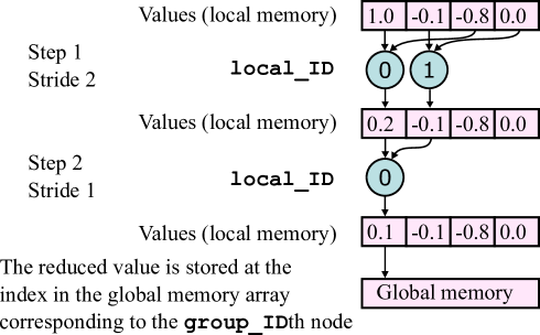
Figure 3: Schematic of binary parallel reduction of a force in one Cartesian direction for one work-group representing the ith of $n$ nodes, for $N=4$.

The OpenCL execution model [46] describes how kernels execute. When a kernel is submitted for execution by the host (as defined in Section 3), an index space is defined. An instance of the kernel, called a work-item, executes for each point in this index space. The work-item can therefore be identified by its point in the index space, called the global_id. Returning to the binary parallel reduction example in Listing 1, to create the index space, each bond in the sparse two-dimensional index set $\{\mathcal{H}_{1},...,\mathcal{H}_{n}\}$ is assigned a $\texttt{global\_id}\in[0,\texttt{global\_size})$, where $\texttt{global\_size}=nN$.

In OpenCL, work-items are organised into work-groups. The work-groups provide a coarse decomposition of the index space. The local_size is the number of work-items per work-group. A work-group is identified by its point in this coarse index space, called the group_id. Thus, each and every node may be assigned a group_id if each work-group contains $\texttt{local\_size}=N$ work-items, as is the case in PeriPy. Work-items are assigned a unique $\texttt{local\_id}\in[0,N)$ within a work-group such that $\texttt{global\_id}=\texttt{group\_id}\times\texttt{local\_size}+\texttt{local\_id}$. Calculations on the work-item are then for the local_idth bond of the group_idth node. The result of executing Listing 1 means that $N$ work-items (for each work-group) execute in parallel to reduce the bond forces to the node force of a single node which is stored in local_cache[0]. Of course, there must be a local_cache for each work-group that stores the bond forces for the work-group’s node. This is explained by the OpenCL memory model [46] in the next section. $N$ must clearly be a power of two so that a binary parallel reduction can be performed. So, $N=\min_{k}(2^{k})\geq\max_{i}(|\mathcal{H}_{i}|)$ is the minimum power of two, which is larger than (or equal to) the maximum number of neighbours of any one node, such that each bond is assigned a global_ID and the constants that are associated with each bond. For example, the stiffness_corrections factors can be stored in a dense global_size C array. Finally, the first work-item in the work-group, local_id = 0 is used to assign this value in the body_force array and the reduction is complete. It is important to note that not only are each work-item in a work-group executed in parallel, but many work-groups can be executed in parallel, also. See that this means we are using the execution model to parallelise over bonds as well as nodes.

As well as using the execution model to perform the binary parallel reduction algorithm, we use the execution model to calculate the other computationally expensive part, the bond-forces. Each work-item is responsible for calculating the bond force of one bond, which is presented in the pseudocode of Algorithm 2 in the Appendix. This is in contrast to the work of Mossaiby et al [28], who assign an index space only over nodes, which is presented in pseudocode in Algorithm 3, also in the Appendix. In the kernel for Algorithm 2, work-items and work-groups are assigned unique global_id and group_id respectively in exactly the same way as in Listing 1. The index of the child node is $j=\texttt{nlist}[\texttt{global\_id}]$, where nlist is the neighbour list and is an $n\times N$ C array where the $i$th row contains $\mathcal{H}_{i}$. The rows of nlist are padded with values of $-1$, where $|\mathcal{H}_{i}|<N$. Note that node indices are taken from the set of non-negative integers, so $-1$ is a safe choice for denoting a broken bond. The global_idth bond is broken by setting the value of $\texttt{nlist}[\texttt{global\_id}]=-1$ and the bond force $f_{ij}=0$. Using Algorithm 2, it is possible to achieve particular optimisations that result in a significant speedup in the peridynamics code, as explained in Sections 3.3-3.5.

In OpenCL, the $\texttt{global\_size}=nN$ must be divisible by the $\texttt{local\_size}=N$ because work-items must be divided between work-groups. Recall that there is a one-to-one mapping between group_ids and nodes, and each work-group is responsible for calculating the resultant node force of a single node. Work-groups are executed in parallel on a device’s compute units. There is no way to synchronise the timings of work-groups since, in an application, there are usually more work-groups than hardware to execute them concurrently. As a result, they will be queued to run as compute units become available. Due to the limited number of compute units on any GPU, we can expect the performance of PeriPy to scale linearly with the number of nodes. At smaller problem sizes, the overhead due to memory transfer between the GPU and controlling CPU dominates, while at larger problem sizes the time required for actual computation comprises most of the total wallclock time. This is seen to be the case in Fig. 4, which shows the performance of PeriPy for different values of $N$. All of the benchmarking tests in Fig. 4 and Fig. 7-9 were run on an NVIDIA 2080Ti GPU for various problem sizes $n$. The benchmarking setup is detailed in Section 4. Fig. 4 shows tests for beams that have been discretised with a regular cubic tensor grid, consistent with the majority of the existing literature. The beams were put under some basic boundary conditions, and the tests were displacement controlled, although this does not affect the simulation time. The stable time-step condition derived by Silling and Askari [30] was used.

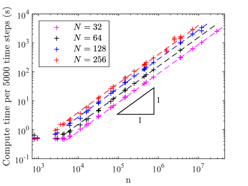
(a) Without stiffness correction factors.

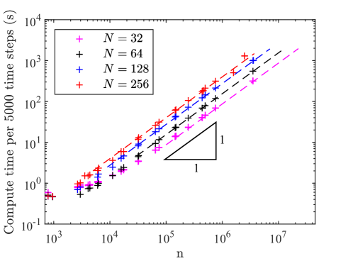
(b) With stiffness correction factors

Figure 4: PeriPy performance across problem size for 5000 time steps with a regular mesh. $n$ is the number of nodes and $N\geq\max_{i}(|\mathcal{H}_{i}|)$ is the maximum number of nodes in the non-local family. A number of problem sizes were used to demonstrate the linear scaling performance of PeriPy for problems with a large number of nodes. The benchmark tests were run on an NVIDIA 2080Ti GPU. The particular geometries and boundary conditions do not affect performance, and simple ones were applied.

Note that $N$ can be chosen independently of $n$. This is because the horizon radius $\delta$ is selected so that it has a value $\delta>m\Delta x$, where $m$ is a small positive constant (usually chosen to be $\pi$) [49] and $\Delta x$ is the mesh spacing. The choices of $m$ and $\delta$ are discussed in Bobaru and Hu [50] and Henke and Shanbhag [51]. In the limit of the horizon $\delta$ approaching zero, the peridynamic solution should converge to the elastic classical continuum mechanics elasticity solution. Bobaru and Hu [50] and Zhao et al. [52] note that the size of the horizon should be defined by the smallest geometrical feature; see also Silling and Askari [30] and Silling and Madenci [53].

3.1.2 Memory model

The memory regions of an OpenCL device and their relationship to the OpenCL platform model [46] are summarised in Fig. 5. The most basic building block of the OpenCL platform model is the processing element: a virtual scalar processor, one of the many concurrent ’threads’ on the device. A work-item may execute on one or more processing elements. A compute unit is composed of one or more processing elements and local memory. An OpenCL device has one or more compute units, and a work-group executes on a single compute unit.

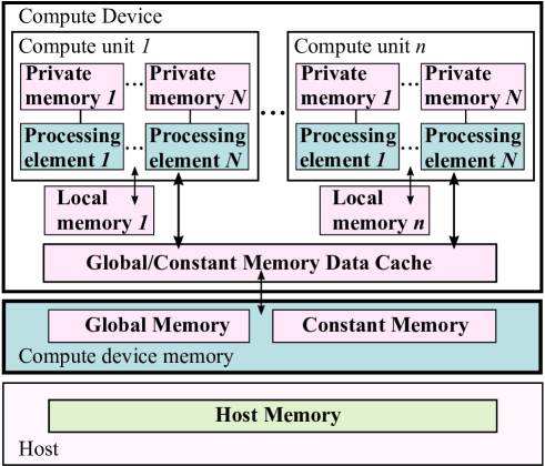
Figure 5: The named address spaces exposed in an OpenCL Platform. Global and Constant memories are shared between the one or more (not shown) devices within a context, while local and private memories are associated with a single device. Each device may include an optional cache to support efficient access to their view of the global and constant address spaces. This figure is adapted from the OpenCL specification [46].

Compute device memory is one or more memories attached to the compute device that are directly available to kernels executing on OpenCL devices. Compute device memory consists of four name address spaces or memory regions:

• Global Memory: permits read/write access to all work-items in all work-groups running on any device within a context. Work-items can read from or write to any element of a memory object. Reads and writes to global memory may be cached depending on the capabilities of the device.

• Constant Memory: A region of global memory that remains constant during the execution of a kernel instance. The host allocates and initialises memory objects placed into constant memory.

• Local Memory: A memory region local to a work-group. This memory region can be used to allocate variables that are shared by all work-items in that work-group.

• Private Memory: A region of memory private to a work-item. Variables defined in one work-item’s private memory are not visible to another work-item.

Local and private memories are always associated with a particular compute unit and processing element, respectively. Local and private memories are much faster than global memory. Therefore, it is imperative to exploit the different memory regions in GPU-accelerated programming. Consider again the binary parallel reduction example in Listing 1. The local memory cache was used to store the three (one for each Cartesian direction) $N\times 1$ C arrays containing the bond forces. The summation is performed using the faster bandwidth of the local memory. The bond forces are never stored in the slower-to-access global memory.

The global and constant memories are shared memories between all compute devices, compute units and processing elements. In the binary parallel reduction algorithm, the body_force array is stored in global memory. In the bond force algorithm, the stiffness_corrections are constant and so stored in the constant memory. In PeriPy, a single compute device is used, which can be either the GPU or CPU. The four named address spaces available to a device do not overlap. This is a logical relationship, however, and an implementation may choose to let these disjointed named address spaces share physical memory.

On the GPU, the private memory accessible to each work-item is small in size and is only $O(10)$ (32-bit) words per work-item and very fast [54]. Non-pointer variables are stored in the private memory, such as those used to assign the node indices $i=\texttt{group\_id}$ and $j=\texttt{nlist}[\texttt{global\_id}]$ and relative displacements $\bm{\xi}_{ij}$. Private memory is used to do fast floating-point arithmetic, such as evaluating the bond force. Each work-group contains many work-items that share its local memory. This memory is larger ($O(10)$ kBytes) than the private memory of a work-item and is used in PeriPy to store the bond forces. The largest memory on a GPU is the global memory, which can be in the high-speed GPU memory (VRAM).

3.2 Hardware considerations

There are a number of hardware-dependent considerations that users of PeriPy should note. These are:

Memory bandwidth: Memory transfers to CPU are expensive, and thus the whole application is transferred onto the GPU until completion unless intermediate writes are performed.

Local memory size: For application to the vast majority of 3D problems in the literature, the $\texttt{local\_size}=N$ is usually $64$, $128$ or $256$ depending on $m$ and, as mentioned above, is a power of two so that a parallel binary parallel reduction can be performed. This can work well since, for NVIDIA cards, which are multiprocessor units that create, manage, schedule and execute threads in groups of 32 parallel threads called warps [55], any local_size that is a multiple of $32$ should result in good thread utilisation. These are also the recommended local_size for intel CPUs [56], in the event the code is to be run on a CPU. The amount of local memory used by a work-item will be the limiting factor of the number of work-items that can be executed in parallel [46], as each work-group offers a limited amount of shared local memory and registers. As a result, the hardware limit on the value of $N$ is CL_KERNEL_WORK_GROUP_SIZE for the kernel that calculates bond forces, which is hardware dependent. On modern cards, this number will be well above the number needed for peridynamics simulations, so is not a problem.

Global memory size: The upper limit on the problem size possible for peridynamics simulations on GPUs is governed by the size of the global memory. The total number of bytes of arrays that are allocated space or stored on the GPU must be less than the size of the global memory. The global memory is used to store the state variables, such as displacement $\texttt{u}[i]=\bm{u}_{i}$ and nlist arrays. If a simulation uses stiffness correction factors, they are stored in an $n\times N$ double C array in the global memory. The constants, such as node coordinates $\texttt{coords}[i]=\bm{x}_{i}$ and volumes $\texttt{vols}[i]=dV_{i}$, are stored in a memory region of global memory called the constant memory, which remains constant during the execution of a kernel. The host allocates and initialises memory objects placed into constant memory. Work-items have read-only access to these objects. These values can be used to approximate the maximum problem size $n$ for a given amount of global memory. The upper limits on $n$ for the NVIDIA 2080Ti GPU with 11Gb of VRAM are shown in Table 1. These values define the upper bound for the problem size in the benchmarking results in Section 4. The approximate calculations used to determine the maximum problem size in PeriPy are shown in Table 5 in the Appendix.

Table 1: Approximate maximum problem size in millions ($10^{6}$) of nodes $n$ for a PeriPy simulation on a GPU with 11Gb of VRAM and work-group size $N$.

Features used in peripy.model class	$N=64$	$N=128$	$N=256$
single material, linear damage model, no stiffness corrections	29.8	18.1	10.1
single material, linear damage model, stiffness corrections	13.0	7.0	3.7
multiple material, n-linear damage model, no stiffness corrections	13.0	7.0	3.7
multiple material, n-linear damage model, stiffness corrections	8.3	4.4	2.2

Precision: Single precision performance (in FLOPS) on GPUs is better than double precision performance [57]. Our tests showed that using single precision with PeriPy is between 6.7 and 8.6 faster than using double precision on our GPU. Now that the memory model has been explained, the optimisations of the current work are demonstrated.

3.3 Optimisation 1: Kernel fusing

Each kernel launch has some overhead, which includes the allocation of memory for the first launch, copying the values of the input parameters to constant memory, indexing any local or global arrays used within the kernel and calculating intermediate variables, such as the bond stretch $s$. By fusing the kernels for calculation and summation of bond forces, the extra overhead is eliminated and the total run time reduced. It is also possible to fuse the kernel that checks whether a bond has exceeded the critical stretch into the bond force calculations kernel, which avoids the need to calculate the bond stretch $s$ twice as well as the need to store the bond forces in an $n\times N$ C array in global memory, which would be accessed by the separate check-bonds kernel. Since there is a work-item for each bond, there are no race conditions that result from fusing these kernels.

The check for broken bonds is applied directly after a displacement update and before the calculation of bond forces. It is important to ensure that all of the bond forces are updated for a given time-step before the time integration is performed to avoid race conditions. Therefore, it is not possible to fuse the time integration kernel with the bond force kernel. Splitting the time integration and bond force kernels guarantees that bond forces are calculated with nodal displacements from the same time step, and vice versa. The time integration kernel for velocity-Verlet is shown in Algorithm 4 in the Appendix.

3.4 Optimisation 2: Parallel reduction of bond forces onto nodal forces

The implementation of binary parallel reduction was explained in Section 3.1. The reduction is needed to reduce the bond forces to the node force. The binary parallel reduction facilitates the parallelisation over bonds as opposed to nodes, which leads to the most significant optimisation of the current work, minimising thread divergence.

3.5 Optimisation 3: Thread divergence

The most significant performance consideration relates to the execution of threads or work-items [58]. Recall that work-items are organised into work-groups. Work-groups can be executed by the GPU in any order, but work-groups are not necessarily execution units themselves. Instead, work-groups are partitioned into warps for execution. In the current generation of NVIDIA devices, each warp consists of 32 threads. If a work-group consists of more than 32 work-items, the work-group is partitioned into multiple warps based on the work-item ID (e.g. local_id). All work-items in a warp should follow the same instruction path. Otherwise, work-items execute different instructions, which is called thread divergence and reduces performance significantly. To avoid thread divergence, work-groups should be organised so that warps follow the same control paths. In the case of Algorithm 3 in the Appendix, thread divergence occurs when, as is most often the case, the number of non-broken bonds between nodes differs. The warp will not complete until all work-items in that warp have completed the for loop starting at line 5. This results in many threads in the warp being under-utilised during that time. However, in PeriPy, Algorithm 2 in the Appendix, the parallelisation is over bonds, and so the time that threads are underutilised is limited to the amount of time it takes to calculate a single bond rather than a number of bonds.

The problem of thread divergence has not been eliminated in Algorithm 2. For example, if some work-items in warp execute the if statement in an if-then-else construct on lines 4-16 (calculating the bond force) while others follow the else path (the bond is broken), the GPU can no longer execute the work-items concurrently, and multiple passes are required. It is not possible to prevent thread divergence and to fuse the kernel that checks if a bond has exceeded the critical stretch into the kernel that calculates the bond force, as both the if and the else paths of the control loop will be executed by many work-items. Clearly, there is a trade off in the performance gain between kernel fusing and preventing thread divergence. Preliminary tests showed that kernel fusing at the cost of thread divergence in this manner is the faster approach across all problem sizes, by two orders of magnitude for large problem sizes $n>10^{6}$. This is because it avoids the memory constraints relating to storing bond forces in an $n\times N$ C array in global memory at every time step, the bandwidth constraints of accessing this array in a separate check-bonds kernel and the need to calculate the bond stretch, $s$, two times.

Increasing $n$ by a factor of 2 will double the amount of warps that need to be scheduled and executed and will thus decrease performance by a factor of 2. The amount of warps that need to be executed per node will be the dominant factor for per-node performance. Increasing $N$ by a factor of 2 will double the number of warps that need to be executed and thus decrease performance by approximately a factor of 2. This relationship is approximate since not all warps take equal time to execute; for example, warps that contain all broken or ’padding’ bonds will take much less compute time to execute compared to warps with non-broken bonds.

3.6 Overview of Code Design

The class diagram for PeriPy is presented in Fig. 6 and shows the peripy.model.Model class, which allows users to define a bond-based peridynamics model for composite materials with non-linear damage models defined by an arbitrary number of linear splines, such as the trilinear damage model illustrated in Fig. 12. Surface correction factors, partial volume correction factors, different micromodulus functions and boundary conditions can be readily included by supplying the relative keyword arguments to the model class. The model is defined by a damage model, the set of keyword arguments described above, a set of initial conditions (coordinates, connectivity and, optionally, node state vectors), force and/or displacement controlled boundary conditions and a set(s) of nodes the user has chosen to measure a datum for. The design of the code has facilitated the following features.

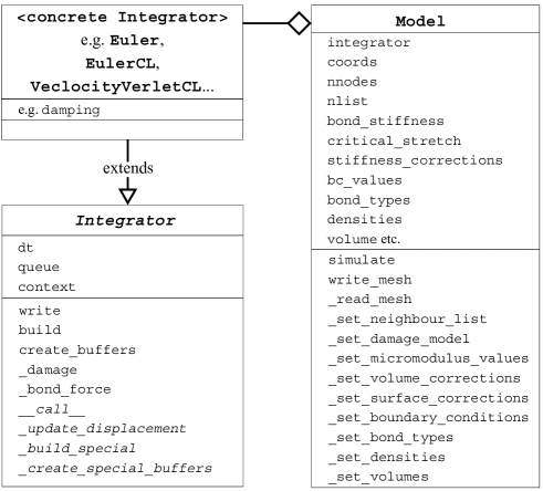
Figure 6: The class diagram for PeriPy, which is designed to easily extend the code with new integrators, correction algorithms or disretisations. The functionality of the code is defined in two classes: Integrator, which is the Abstract Base Class (ABC) that is extended by a concrete Integrator class, such as EulerCL, and Model, which defines the geometry (mesh and node volumes), connectivity (neighbour list and number of neighbours for each node), damage model, material types, correction algorithms and boundary conditions.

Readily extended integrators: When instantiating the peripy.model.Model class, an explicit integrator that inherits peripy.integrators.Integrator as an Abstract Base Class is required. PeriPy has not yet been extended to implicit integration methods, and contributions are welcome. Examples of the explicit integrators included are: peripy.integrators.Euler, peripy.integrators.EulerCL, peripy.integrators.EulerCromerCL and peripy.integrators.VelocityVerletCL. The suffix CL represents an integrator that utilises OpenCL kernels. As mentioned earlier, the CL integrators can be utilised on any CPU or GPU platform due to the heterogeneous nature of OpenCL.

Regular and irregular meshes: PeriPy uses the python package meshio [59] to read input meshes of various formats, where the vertices of the meshes are the peridynamic nodes. PeriPy can take cuboidal tensor grid meshes as input, which are often employed so that the nodal volumes $dV_{i}$ can be easily and accurately calculated. Regular or irregular tetrahedral grids may also be used, with the only complication being the need to define a volume associated with each node. This may be accomplished by using computational geometry techniques, such as Delaunay triangulation or Voronoi diagrams [60], which are not included in the package. Instead, if a tetrahedral mesh is used and exact nodal volumes are not supplied through the keyword argument volume of the model class peripy.model.Model, Peripy will approximate the nodal volumes by a weighted sum of the volumes of the tetrahedra of which the node is a vertex. Specifically, if a node is a vertex of a tetrahedra, it will be assigned 1/4 of the volume of that tetrahedra. The volumes of the tetrahedra are calculated using the standard formula of a dot product and cross product of the difference of the vertex position vectors. With this method, the total sum of the nodal volumes is equal to the total volume of the mesh, and as the volumes go to zero the absolute error is reduced. In the case of a regular cuboid grid that is split into tetrahedra, as the mesh elements are congruent, this method will result in exact volumes in the bulk. However, on the boundaries there will always be a significant error in the volumes when compared to the Veronoi diagram method. This results in surface nodes that have different effective stiffnesses to the bulk and will cause surface effects extraneous to the ‘peridynamics surface effect’ explored by Le and Bobaru [43]. It is therefore recommended that, if an irregular mesh is used and the exact volumes are known, then they should be supplied through the keyword argument volume. While both irregular and regular tetrahedral meshes are possible with PeriPy, for the purposes of this paper, regular cuboidal tensor grid meshes were used, keeping with the majority of the existing literature.

Composite materials: Composite materials and structures can be defined and supplied to the peripy.model.Model class.

General boundary conditions: General boundary conditions can be supplied, and magnitudes of the boundary conditions can be changed over time. The directions of the boundary conditions cannot be changed over time, except along the directions that they were initially defined. This means that, while most commonly used boundary conditions are possible, torsion, for example, is not currently possible; however, contributions are welcome.

Reduced overhead: The neighbour list generated using the scipy.spatial.KDTree class [61]. In PeriPy, the arrays that are constructed during the instantiation of the peripy.model.Model, such as the neighbour list, can be written to an h5 [62] file and read by the peripy.model.Model through keyword arguments. This reduces the overhead needed to simulate an example.

Running simulations: Simulations are conducted with Model.simulate. The peridynamics parameters of a damage model, node states, initial conditions and boundary conditions can be changed without reinstantiating the peripy.model.Model by setting them as keyword arguments to the peripy.Model.simulate method. In this way, multiple simulations with different parameters be conducted with minimal overhead cost so that ’outer loop’ applications, including sensitivity analysis, uncertainty quantification and optimisation, may be performed.

Initiating a simulation from an intermediate state: The peripy.model.simulate can be restarted from an intermediate state by supplying a first_step argument and state variables for that time step. This could be useful, for example, when changing parameters that do not affect the elastic response of the model but do affect the crack nucleation and propagation, in which case the simulation states would be saved in the linear elastic region of a quasi-static response of an increasing load.

Output visualisation in ParaView: The simulate method will write the states to a mesh file that is easily visualised (e.g. Paraview [63]). Writes occur at a specified frequency, in a number of steps. The other outputs of the method are a tuple of the state vectors and a dictionary object containing the average of displacement, velocity and acceleration as well as the sum of forces and body forces for each of the writes (over time), for each unique tip_type, which is defined as the set of nodes the user has chosen to measure a datum for, as defined by the is_tip function. This could be the set of nodes on the tip or midspan of a structure.

For a comprehensive explanation and usage of all classes, methods and arguments, please see the latest full documentation at https://peripy.readthedocs.org.

4 Benchmarking

This section will compare the performance of the solver versus two existing solvers. One is an OpenMP implementation by Hobbs [64]. All the functions are written in C and use OpenMP. The C functions are called directly by MATLAB. This requires compilation of the C code into a MEX function (MATLAB executable). The compilation used gcc-6.3.0 for Linux and the MATLAB version used was R2018b. The computations were performed using a single Skylake node with 32 OMP threads with the Cambridge Service for Data Driven Discovery (CSD3) Peta4 platform operated by the University of Cambridge Research Computing Service. The other solver is the OpenCL implementation by Mossaiby et al. [28]. The source code provided by Mossaiby et al. [28] was executed by us along with the OpenMP and PeriPy codes. Both OpenCL solver computations were run on an NVIDIA 2080Ti with 11GB GDDR6 RAM and 4352 CUDA cores, and pyopencl==2020.1 was used.

The results show a 1.4-2.0x performance gain over the OpenCL solver, with an up to 10.0x performance increase for problems with a small number of nodes $n$. The results also show a 3.7-7.3x performance gain over the OpenMP solver. Linear compute scaling across problem size $n$ (number of nodes) and family size $N$ is demonstrated. There is a negligible difference in the performance of PeriPy as a result of using stiffness correction factors.The performance difference of using an irregular mesh rather than a regular mesh is shown and an explanation provided.

4.1 Comparing across problem size, and horizon distance

The performance of PeriPy across problem size with and without any stiffness correction factors is shown in Fig.4. The performance depends on the number of warps that need to be executed on the device. The performance is linear with the number of nodes $n$ and approximately linear with the family size $N$, for the reasons discussed in Section 3.5.

The performance with irregular meshes is shown in Fig.7. For the same $N$, performance for the irregular meshes is faster than with regular meshes. This is because, in irregular meshes, the range of the family size $|\mathcal{H}_{i}|$ across the node index $i$ is larger than in a regular mesh, so the group_size, $N=\min_{k}(2^{k})\geq\max_{i}(|\mathcal{H}_{i}|)$, is typically 2 times larger than the regular mesh with equivalent average spacing $\Delta x$. As a result, there are whole warps in the irregular mesh case for which no bond force calculations are required, which are performed much faster time than warps for which a bond force calculation is required. As a result, the performance for an $N=64$ irregular mesh closely matches that of $N=32$ with a regular mesh; the performance for an $N=128$ irregular mesh closely matches that of $N=64$ with a regular mesh and so on, as shown in Table 2.

Table 2: The number of additional nodes to increase the wall clock time of 5000 time steps by one second, $\frac{\partial n}{\partial t}\bigg{|}_{N}$.

N	Regular mesh	Irregular mesh
$32$	$11487$
$64$	$6452$	$13341$
$128$	$3652$	$5532$
$256$	$2500$	$3990$

The effect on performance of using stiffness correction factors (i.e. through micromodulus function, partial volume correction or surface corrections) is negligible, except at small problem sizes. At smaller problem sizes, the overhead due to memory transfer between the GPU and controlling CPU dominates, and copying the stiffness correction factor C array buffer onto GPU impacts performance. At larger problem sizes, the time required for actual computation comprises most of the total wallclock time, and the only change in the computation is the indexing of a constant stiffness correction factor array, which does not significantly impact performance.

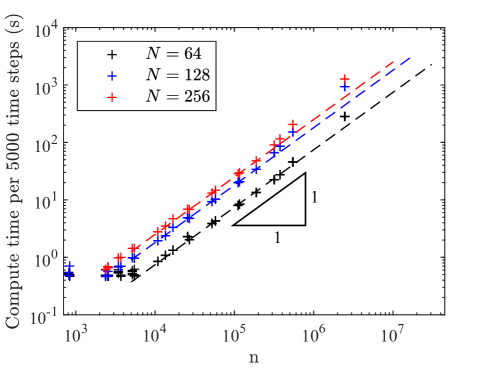
(a) Without stiffness correction factors.

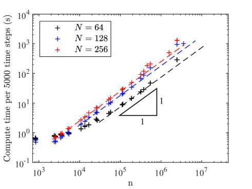
(b) With stiffness correction factors

Figure 7: PeriPy performance across problem size for 5000 time steps with an irregular mesh. $n$ is the number of nodes and $N\geq\max_{i}(|\mathcal{H}_{i}|)$ is the maximum number of nodes in the non-local family. A number of problem sizes were used to demonstrate the linear scaling performance of PeriPy for problems with a large number of nodes. The benchmark tests were run on an NVIDIA 2080Ti GPU. The particular geometries and boundary conditions do not affect performance, and simple ones were applied.

4.2 Comparing against existing solvers

The performance of PeriPy when compared to the OpenCL solver by Mossaiby et al. [28] is shown for the group_size $N=128$ in Fig. 8(a), and with the added comparison against the OpenMP solver by Hobbs it is shown for the group_size $N=256$ in Fig. 8(b). The speedups identified in Section 3 result in PeriPy being 1.4-2.0 times faster than the OpenCL solver by Mossaiby et al. [28] and 3.7-7.3 times fast than the OpenMP solver by Hobbs. As explained in Section 3.5, the speed increases are a result of (1) kernel fusing of the calc_bond_force and check_bonds kernels, (2) parallelisation over bonds (as opposed to nodes), which facilitates the most significant performance enhancement which is (3) minimisation of thread divergence. The relative effect on the performance of the speedups and a detailed explanation are provided below.

Fig. 9 shows the effect of binary parallel reduction (PeriPy BPR) on performance when compared to a serial reduction (PeriPy SR). Mossaiby et al. (2017) do not include any of the optimisations, while PeriPy SR has optimisations (1) but not (2) or (3). The speedup due to (1) is significant and is shown by the difference between PeriPy SR and Mossaiby et al.

The logical implications of the results in Fig. 9(a) are that the summation algorithm, parallel or serial, does not actually yield much performance gain in and of itself. Rather, the binary reduction facilitates the parallelisation over bonds without needing to store a huge bond forces array in the GPU global memory every time step in order to do a summation of bond forces. The majority of the time savings for regular meshes is a result of kernel fusing.

However, it is for the irregular mesh, as shown in Fig. 9(b), that the speedups due to (2) and (3), which are implemented in PeriPy BPR, are fully realised. These speedups are primarily due to reducing thread divergence to a practical minimum by parallelising over bonds rather than nodes. Consider, as is the case in PeriPy SR, parallelising over nodes. Each work-item, corresponding to a node, has to calculate the force of non-broken bonds for that node. It is often the case for irregular meshes that the number of non-broken bonds between each node varies significantly. Therefore, parallelising over nodes results in significant thread divergence, which depends on the range of broken bonds for the nodes. In PeriPy BPR, we reduce the thread divergence as much as possible by parallelising over bonds. The only thread divergence left is whether or not the bond force for a bond is calculated, and hence we achieve the minimum possible thread divergence for the problem, which results in the speedup. This explains why the performance of PeriPy for irregular meshes is much better than in Mossaiby and the PeriPy SR implementation.

It can also be seen from Fig. 9 that, for small problems, where the overhead due to memory transfer between the GPU and controlling CPU dominates, PeriPy BPR is up to 10 times faster than Mossaiby et al. and PeriPy SR. The difference between PeriPy SR and PeriPy BPR is that the parallelisation is over bonds rather than nodes (2), and so forces are calculated in local rather than global memory, reducing communication time, and the thread divergence is also reduced (3).

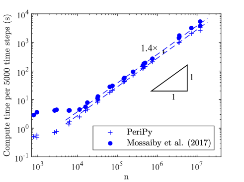
(a) $N=128$, regular mesh

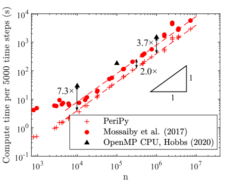
(b) $N=256$, regular mesh

Figure 8: Comparison across different implementations for 5000 time-steps with a regular mesh.

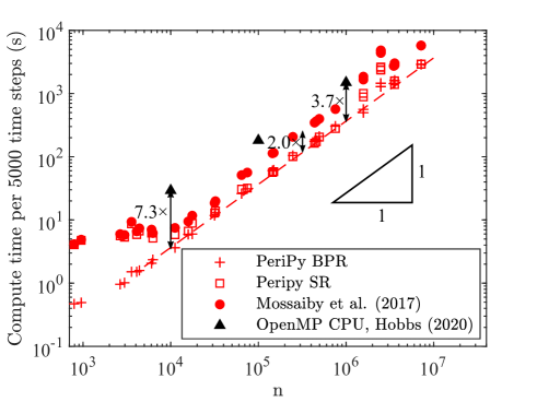
(a) $N=256$, regular mesh

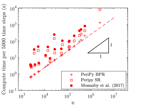
(b) $N=256$, irregular mesh

Figure 9: Irregular mesh versus regular mesh comparison across different implementations for 5000 time-steps.

5 Validation of PeriPy through engineering test cases

In this section we demonstrate the use of PeriPy for explicit schemes for a 3D dynamic test. In testing, PeriPy was also validated against other solvers for simple test cases.

5.1 Example 1: Kalthoff–Winkler experiment

The Kalthoff–Winkler experiment [65] [66] is a classical benchmark problem for dynamic fracture [67, 68, 69]. The geometry and boundary conditions used for the simulation are illustrated in Fig. 10. The thickness of the specimen is $9\text{\,}\mathrm{mm}$. For a plate made of 18Ni1900 steel subject to impact loading at the speed of $v_{0}=$32\text{\,}\mathrm{m}\text{\,}{\mathrm{s}}^{-1}$$, brittle fracture was observed with a crack forming at $68\mathrm{°}$ angles to the notches. We repeat the simulation first conducted by Silling [70] and repeated by Ren et al. [10] using the same material parameters as in the latter, comparing our results for validation purposes. The elastic modulus is $E=$190\text{\,}\mathrm{GPa}$$, the density is $\rho=$7800\text{\,}\mathrm{kg}\text{\,}{\mathrm{m}}^{-3}$$, Poisson’s ratio is $\nu=0.25$ and the energy release rate is $G_{0}=$6.9\text{\times}{10}^{4}\text{\,}\mathrm{J}\text{\,}{\mathrm{m}}^{-2}$$. Repeating the experiment by [10], impact loading was imposed by applying an initial velocity at $v_{0}=$22\text{\,}\mathrm{m}\text{\,}{\mathrm{s}}^{-1}$$ to the first three layers of nodes in the domain, as shown in Fig. 10; all other boundaries are free. The plate is discretised with a node diameter $\Delta x=$1.5625\text{\,}\mathrm{mm}$$. Along the thickness of the plate, four layers of nodes are employed to match the simulation in [10]. The total number of nodes is $n=32,768$.

We also repeat the simulation conducted by Mossaiby et al. [28] in the validation of their solver, using material parameters the same as in the study by Ren et al. [10], but, following Mossaiby et al. [28], the plate is discretised with a node diameter of $\Delta x=$1.0\text{/}2560\text{\,}\mathrm{m}$$, with $13$ layers of nodes, contributing to the total number of nodes $n=1,713,933$.

It should be noted here that, in order to prevent crack nucleation at the centre of the long edge away from the pre-cracks, a ‘no failure zone’ must be imposed on that edge, as can be seen in the simulation of [10]. If no ‘no failure zone’ is to be used, then a micro-elastic plastic damage model must be used, as mentioned by Silling [70]. The ‘no failure zone’ is simple to implement in PeriPy and results in a fracture pattern that matches the simulations by Ren et al. [10] and Mossaiby et al. [28], the latter of which is shown in Fig. 11 (right).

The crack propagation speed is given as

$$\|\dot{u}(t+\frac{\Delta t}{2})\|=\frac{\|\bm{x}_{\text{tip}}(t+\Delta t)-\bm{x}_{\text{tip}}(t)\|}{\Delta t}$$ (16)

where $\bm{x}_{\text{tip}}(t)$ is the position of the crack tip at time $t$. The Rayleigh wave speed $c_{R}$ [71] is given as

$$\frac{c_{R}}{c_{s}}=\frac{0.87+1.12\nu}{1+\nu}$$ (17)

where $c_{s}=\sqrt{\mu/\rho}$ is the shear wave speed, and $\mu$ is the shear modulus.

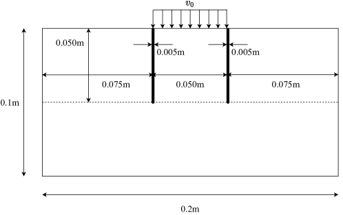
Figure 10: Setup of Kalthoff–Winkler’s experiment.

The crack tip is measured using the corner detection algorithm developed by Harris[72] with the OpenCV python package [73]. Corner detectors can be unreliable, and higher-level visual routines must be designed to tolerate a significant number of outliers in the output of the corner detector. Outliers were filtered if the resulting velocity was above the Rayleigh speed, and the results were averaged with slightly different values for the free parameter $\kappa$, which describes how ‘edge phobic’ the corner detection algorithm is. Fig. 11 shows the evolution of the crack speed using this method. The speed was calculated every $5\text{\times}{10}^{-6}\text{\,}\mathrm{s}$. For verification purposes, our results are compared with those of the peridynamic model in [10].

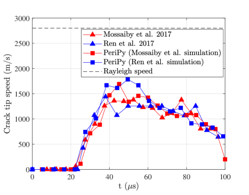
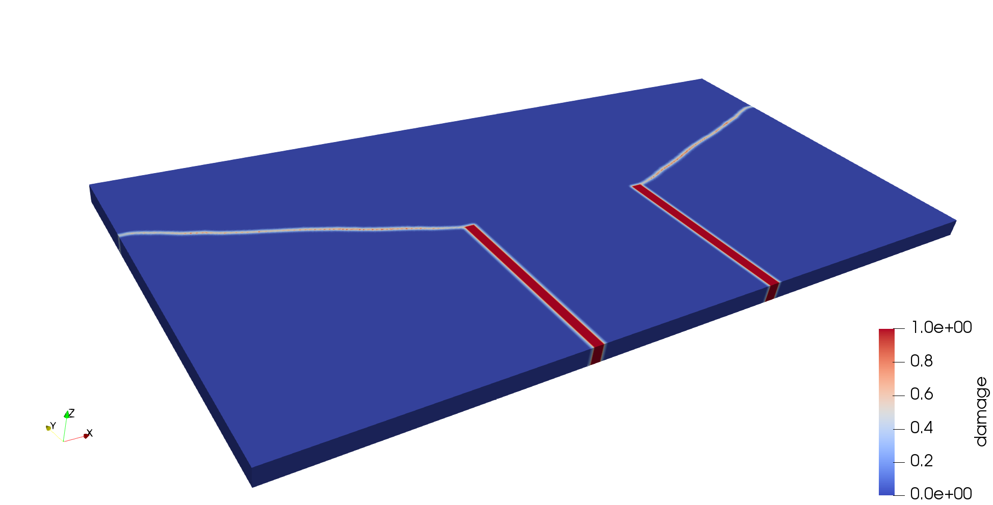
Figure 11: (Left) The crack propagation speed in Example 2. (Right) The crack at $100\text{\,}\mathrm{\SIUnitSymbolMicro s}$ as viewed as a mesh file in ParaView [63].

The crack starts to propagate at $24\text{\times}{10}^{-6}\text{\,}\mathrm{s}$, the same time as in the simulation of Ren et al. [10] The highest crack speed in the simulation measured by the corner detection algorithm was $1830\text{\,}\mathrm{m}\text{\,}{\mathrm{s}}^{-1}$, $65.4\%$ of the Rayleigh speed, which was larger than Ren’s value of $1500\text{\,}\mathrm{m}\text{\,}{\mathrm{s}}^{-1}$. Most other velocities are in good agreement. The crack angle at the kink was measured to be $65.3\mathrm{°}$, closely matching Ren’s reported value of $65.7\mathrm{°}$.

6 Example 2: Outer-loop calibration of peridynamics model parameters using experimental force-deflection data

This section presents an optimisation problem to calibrate a bond-based trilinear damage model for a concrete beam simulation. Concrete is a quasi-brittle material and exhibits strain-softening behaviour when in tension. Yang et al. [74] noted that the tension softening part of the bilinear model, was not based on the true softening behaviour of concrete and thus established a trilinear model within the bond-based peridynamic formulation, illustrated in Fig. 12. The shape of the softening branch in the trilinear model is consistent with the tension softening behaviour of concrete. A generalised method for determining the parameters $s_{0}$, $s_{1}$ and $s_{c}$ was proposed and only requires the elastic modulus, tensile strength and fracture energy. The position of the kink point in the softening curve is determined by the initial fracture energy, as proposed by Bažant [75]. However, the critical stretch of a peridynamic bond is dependent on fracture energy $G_{F}$. The selection of $G_{F}$ is a major source of uncertainty in peridynamic models. Furthermore, concrete material properties are typically determined through the testing of concrete compressive strength $f_{c}$. Additional material parameters, such as elastic modulus $E$, tensile strength $f_{t}$ and fracture energy $G_{F}$, are rarely tested and must be determined from empirical formulas. At present, there is no standard theory relating concrete compressive strength to fracture energy.

Figure 12: Trilinear damage model.

It is therefore likely that an ’outer-loop’ data-driven method, is required to calibrate the trilinear model against experimental data. PeriPy is a useful tool in such outer-loop applications, providing sufficiently fast model evaluates to enable optimisation routines. Following Yang et al. [74], we set the kink point to $\beta=1/4$, and compare the values of the trilinear model of Yang et al. [74] to optimised parameters that are calibrated against experimental data. A schematic diagram of the experimental setup used [76] is illustrated in Fig. 13 (Left). Results for the unnotched (UN), (notch-to-depth ratio $\lambda$ = 0) and fifth-notched (FN), notch-to-depth ratio $\lambda=0.2$ case are presented. The member has the following dimensions: length $l=175$ mm; depth $d=50$ mm; and thickness $b=50$ mm. The span of the member is $125$ mm, and width of the notch is $2$ mm. The beam was tested multiple times, and the range of experimental results are plotted in grey in Fig. 14 for the un-notched case and notched case. The means are plotted in black. The experimental tests are crack-mouth-opening-displacement (CMOD) controlled to avoid unstable crack propagation after the peak load. The unnotched plain concrete beam in three-point bending was used for calibration of point-estimates of the trilinear model parameters. The calibrated point-estimates were then tested on a notched concrete beam and compared to experimental data.

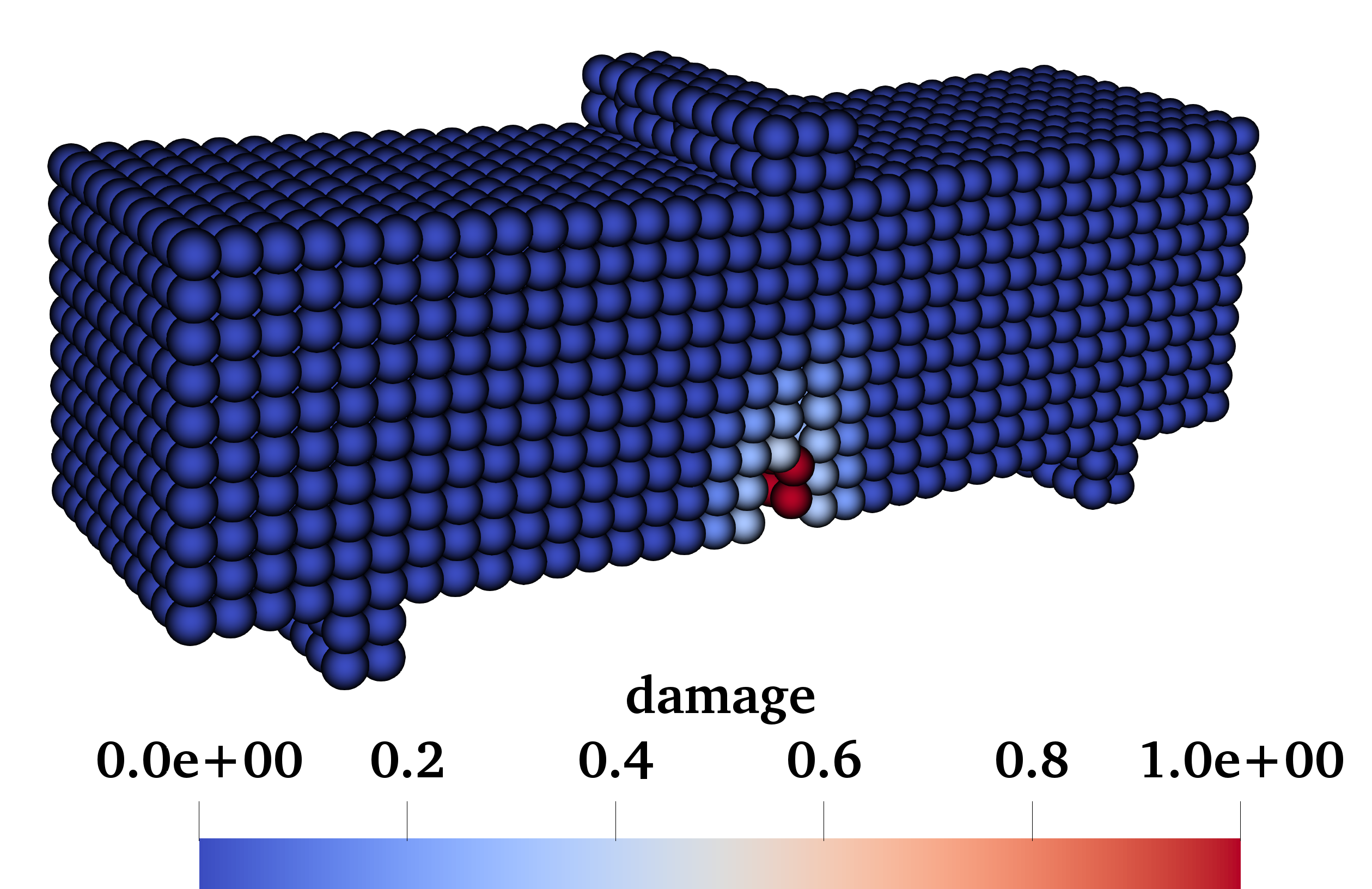
Figure 13: (Left) Schematic of the experimental setup reported by Grégoire et al. [76]. (Right) Peridynamic model of fifth notched plain concrete beams, discretised with a $5\text{\,}\mathrm{mm}$ mesh. The boundary conditions are applied to the peridynamic nodes outside the surface of the beam, and the initial notch is shown in red.

The peridynamic model was discretised using a $\Delta x=$5\text{\,}\mathrm{mm}$$ mesh giving a total number of peridynamic nodes of $n=3,645$. A fixed peridynamic horizon of $\delta=$15.7\text{\,}\mathrm{mm}$$, and no stiffness correction methods were applied in this simulation (see Example 3). A displacement-controlled loading scheme is used for the numerical simulations. The left-hand support was clamped in all three directions. Following the experimental setup closely, the beam was simply supported. The right-hand support was constrained not to move in the vertical and out-of-plane directions. The central support was constrained not to move in the out-of-plane direction and had a prescribed displacement in the vertical direction. As noted by Mehrmashhadi et al. [36], applying imposed displacements to a single node will result in a significant peridynamic surface effect. Boundary displacements were applied over a two-by-two node cross-section outside the surface of the beam (except for the central point load, where the boundary was applied over a three-by-two node cross-section, for symmetry), which is shown in Fig. 13 (right). The boundary nodes were set as ‘no-failure-zones’ so that they do not exceed critical stretch, which would be nonphysical, and their bond stiffness was taken to be the same as the bulk material. The displacement boundary conditions were applied smoothly using a fifth-order polynomial displacement time curve, such that the boundary nodes had an acceleration of zero at the first time step and during crack nucleation and growth. Dynamic damping was used to dampen oscillations in the beam. These steps serve to increase the stability of simulation and ensure that crack growth occurs under quasi-static loading conditions. The exact dynamic parameters used for the simulations and the velocity of the applied displacement in the vertical direction are shown in Table 3. As per the original experimental paper [76], the CMOD was measured by the relative displacement in the $x$ direction of two points, $25\text{\,}\mathrm{mm}$ on either side of the midpoint of the beam. To apply the notch, all bonds that are at least partially within the volume of the void of the notch were broken as an initial condition. The force $P$ was measured as the vertical resultant force in the bonds of the displacement controlled particles.

Table 3: Dynamics parameters for Example 2 and Example 3.

	Example 2	Example 3
$\Delta t$ $\text{\,}\mathrm{s}$	$1.135\times 10^{-6}$	$8.788\times 10^{-7}$
$\eta$ $\text{\,}\mathrm{kg}\text{\,}{\mathrm{m}}^{-3}\text{\,}\mathrm{s}$	$2.5\times 10^{6}$	$2.5\times 10^{6}$
max displacement rate $\text{\,}\mathrm{m}\text{\,}{\mathrm{s}}^{-1}$	$3.5\times 10^{-10}$	$8.0\times 10^{-8}$
final displacement $\text{\,}\mathrm{m}$	$4.4\times 10^{-5}$	$2.7\times 10^{-3}$

In this simple example, calibration of material parameters was performed on the unnotched experiment using a simple binary search. In order to find a point estimates of the bond stiffness $c$, the gradient of the elastic part of the experimental force-CMOD curve was calibrated to the gradient of the simulation force-displacement curve to two significant figures. In order to calibrate the trilinear parameters $s_{0}$, $s_{1}$ and $s_{c}$, a loss function in the form of a mean squared error between the experimental data and the numerical solution was minimised until the parameters converged to two significant figures through successive iterations of binary searches for each parameter.

The results for two possible calibrations, ’Point estimate UN 1’ and ’Point estimate UN 2’ (corresponding to two different minimum values of the loss function used) for the un-notched case are shown in Fig. 14 (left). The values of the calibrated model parameters are compared to values from the trilinear model of Yang et al. [74] in Table 4. The calibrated model parameters were then tested on fifth-notched (FN) beam geometry.

Table 4: optimised parameters of the trilinear model against experimental data.

	Trilinear model Yang et al. [74]	Point Estimate 1	Point Estimate 2
$c$	$2.32\times 10^{18}$	$1.792\times 10^{18}$	$1.792\times 10^{18}$
$s_{0}$	$1.05\times 10^{-4}$	$2.3\times 10^{-4}$	$2.0\times 10^{-4}$
$s_{1}$	$6.90\times 10^{-4}$	$2.42\times 10^{-4}$	$2.42\times 10^{-4}$
$s_{c}$	$5.56\times 10^{-3}$	$1.45\times 10^{-3}$	$1.75\times 10^{-3}$

The trilinear model parameters determined by the calibration of the numerical simulation (’Point estimate UN 1’ and ’Point estimate UN 2’) are compared to the values determined by the trilinear model proposed by Yang et al. [74] in Table 4. The mean material properties of the experimental beam were used to calculate the trilinear model [74] parameters: compressive strength $f_{cm,cyl}=$$42.3\text{\,}\mathrm{MPa}$; modulus of elasticity $E=$$37.0\text{\,}\mathrm{GPa}$; splitting tensile strength $f_{t}=$$3.9\text{\,}\mathrm{MPa}$. The density of the concrete mixture is $\rho=$$2346\text{\,}\mathrm{kg}\text{\,}{\mathrm{m}}^{-3}$. The material fracture energy is determined empirically using fib Model Code 2010: $G_{F}=73f_{cm}^{0.18}=$$143.2\text{\,}\mathrm{N}\text{\,}{\mathrm{m}}^{-1}$.

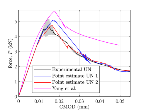
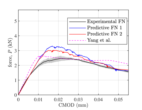
Figure 14: For a $\Delta x=$5\text{\,}\mathrm{mm}$$ mesh, (a) experimental and calibrated curves, achieved by minimising the mean squared error between the experimental displacement plots and two point estimates of the trilinear parameters (coloured) on the un-notched (UN) beam geometry; (b) experimental and predictive curves, achieved by using the calibrated point estimates from the unnotched beam data applied fifth notched (FN) beam, i.e. $\lambda=0.2$

7 Example 3: Predicting the failure load of a reinforced concrete beam

This section presents the large-scale industry-motivated problem of estimating the failure load of a reinforced concrete beam. The numerical and experimental results for a reinforced concrete beam failing in shear, ‘Beam 5’ from the series of reinforced concrete beam tests by Leonhardt and Walther [77], commonly referred to as the Stuttgart Shear Tests.

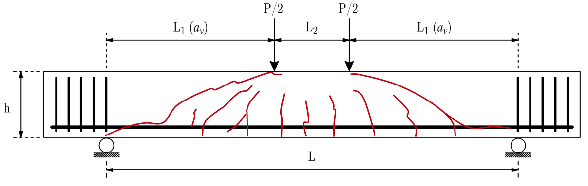
Figure 15: Schematic of the experimental setup. Adapted from Leonhardt and Walther [77]. Final fracture pattern of the experiment shown in red.

The beam is subjected to four-point loading, and shear reinforcement was not present between the applied loads so that the development of diagonal shear cracks could be studied. A schematic diagram of the experimental setup is illustrated in Fig. 15, overlaid by the fracture pattern observed towards the end of the test. The span of the member L = $1950\text{\,}\mathrm{mm}$, and the shear span $a_{v}$ = $810\text{\,}\mathrm{mm}$. The effective depth d, the distance from the top compression fibre to the centre of the tensile reinforcement, is $270\text{\,}\mathrm{mm}$. The cross sectional area is $320\text{\,}\mathrm{mm}$ $\times$ $190\text{\,}\mathrm{mm}$, and the reinforcement ratio, the ratio between the area of steel $A_{s}$ and the total cross-sectional area, is approximately 2.05%. Longitudinal reinforcement is provided in the form of two ribbed steel bars with $26\text{\,}\mathrm{mm}$ diameters. The reinforcing bars were manufactured from high-yield steel, for which we assume the following material properties: modulus of elasticity $E_{s}$ = $208\,000\text{\,}\mathrm{MPa}$, yield strength $f_{y}$ = $465\text{\,}\mathrm{MPa}$. Since the beam fails in shear, the steel was assumed not to yield, and hence it could be modelled with a linear damage model. Input parameters for the concrete constitutive model have been determined using empirical formulas from fib [78], which relate the experimentally measured cubic compressive strength to common concrete properties. The following concrete properties were used: cubic compressive strength $f_{cm,cube}$ = $35\text{\,}\mathrm{MPa}$, material fracture energy $G_{F}$ = $133\text{\,}\mathrm{N}\text{\,}{\mathrm{m}}^{-1}$ and modulus of elasticity $E_{c}$ = $30\,500\text{\,}\mathrm{MPa}$.

The peridynamic model was finely discretised using a $\Delta x=$5\text{\,}\mathrm{mm}$$ mesh with $\delta=$15.7\text{\,}\mathrm{mm}$$. The total number of peridynamic nodes was $n=957,002$. A displacement-controlled loading scheme was used for the numerical simulations. Following the experimental setup closely, the beam was supported such that the right-hand support was constrained not to move in the vertical and out-of-plane directions. The left-hand support was clamped. The central supports were constrained not to move in the out-of-plane direction and had a prescribed displacement in the vertical direction. For the reasons outlined in Section 6, the boundary displacements were applied over two-by-two node cross-sections outside the surface of the beam at the positions of the arrows and supports on Fig. 15. These nodes were set as ‘no-failure-zones’ so that they do not exceed critical stretch, which would be nonphysical, and their bond stiffness is the same as the bulk material. The displacement boundary conditions were applied smoothly over a fifth-order polynomial displacement time curve such that the boundary nodes had an acceleration of zero at the first time step and during crack nucleation and growth. This ensures that crack growth occurs under quasi-static loading conditions. The exact dynamic parameters used for the simulations and the maximum displacement rate of the applied displacement in the vertical direction are shown in Table 3.

In this simulation a bilinear damage model originally proposed by Gerstle et al. [79] was used. Zaccariotto et al. [80] determined the parameters of the bilinear damage model with material fracture energy $G_{F}$ and experimental load-displacement curves. The energy required to start the fracture process is defined as $G_{0}$ and $k_{r}=s_{c}/s_{0}=G_{f}/G_{0}$. The stretch at the linear elastic limit $s_{0}$ given by

$$s_{0}=\sqrt{\frac{5G_{0}}{6E\delta}}$$ (18)

and $k_{r}$ is determined from experimental load-displacement curves or through sensitivity studies. Stiffness correction factors were applied to this numerical simulation. The force $P/2$ was measured as the vertical resultant force in the bonds of the displacement-controlled particles. The midspan deflection was measured as the average deflection of the nodes at the top of the beam at the midspan ($975\text{\,}\mathrm{mm}$ from the left-hand support).

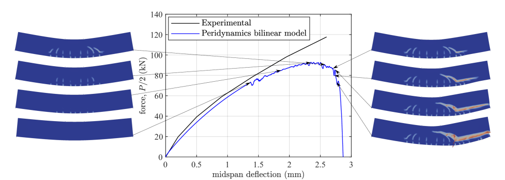
Figure 16: Comparison of load vs. midspan deflection for Beam 5 between experimental data and the bilinear peridynamic model results. The experimental data is from Leonhardt and Walther [77]. The deflection visualisation is amplified 50 times.

A comparison between the force-deflection curve generated from model and experiment is shown in Fig. 16, alongside inset plots show the evolution of the fracture pattern in the simulations. Without specific calibration of the damage model parameterisation for this test, the numerical and experimental model show good qualitative agreement. The numerical solution underestimates failure, and demonstrates a more progressive damage response to failure. The peridynamic model reproduces the expected asymmetrical failure mode, note that in both cases as the diagonal crack propagates into the compression zone, the characteristic rotation behaviour is seen. The final full crack is shown in a Paraview visualisation in Fig. 17. Further improvements to the modelling of this specific experiment could be achieved by refining the model representation, application of loading and boundary conditions, and exploring different material models. Here however, the example demonstrates the scale of peridynamic solutions which can be readily solved using PeriPy.

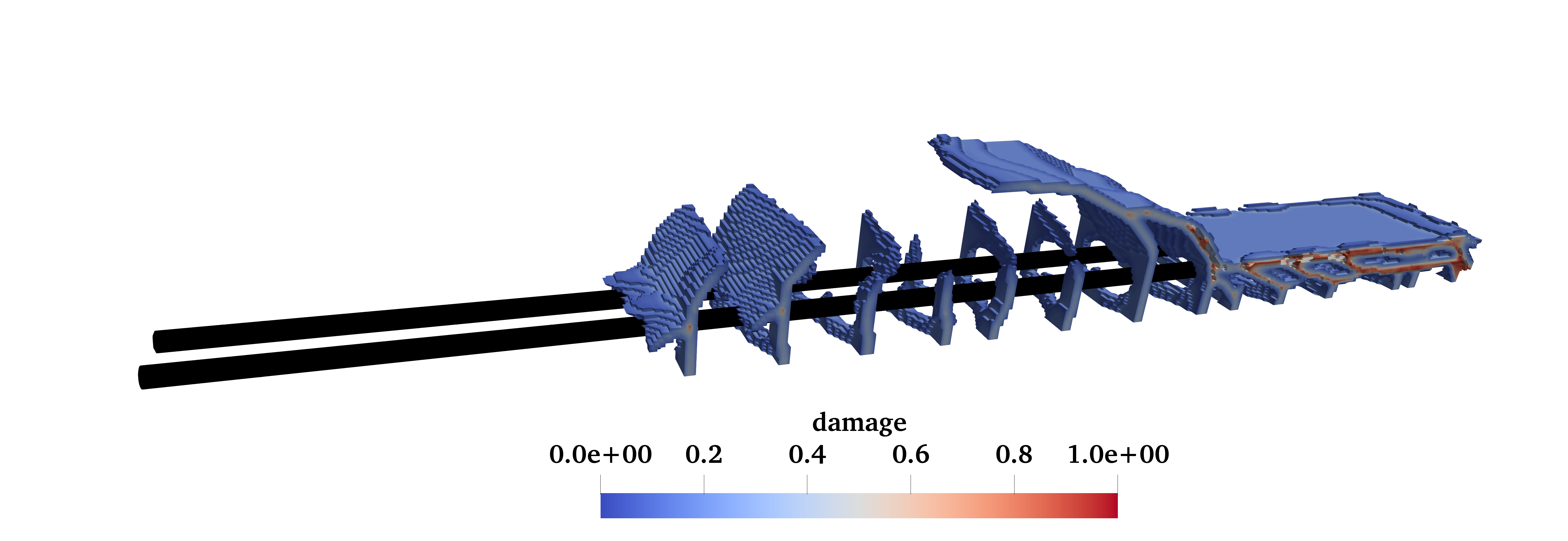
Figure 17: Threshold plot of peridynamic damage, showing three-dimensional visualisation of fracture pattern. The steel rebar nodes are contained in the black cylinders.

8 Future developments

This section outlines some possible extensions to the code. The user is encouraged to file bug reports or feature requests and make contributions by opening a ‘new issue’ on GitHub (https://github.com/alan-turing-institute/PeriPy/issues).

8.1 Stiffness correction algorithms

The code has been developed to be easily extendable. Any partial volume algorithm, stiffness correction algorithm or micromodulus function can be applied with only minor changes to the code.

8.2 State-based Peridynamics

While PeriPy is currently a bond-based peridynamics solver, it may be extended using the same ideas to ordinary state-based (OSB) peridynamics. In OSB peridynamics, the bond force $\bm{f}_{ij}$ of one bond $\bm{\xi}_{ij},j\in\mathcal{H}_{i}$ is not in general independent of another bond $\bm{\xi}_{ik},j\in\mathcal{H}_{i}$ within the horizon. However, the individual components needed to calculate $\bm{f}_{ij}$ are calculated in two nested for-loops [81]: one to calculate a ‘nodal dilation’ using $\bm{\xi}_{ij},j\in\mathcal{H}_{i}$ and $\bm{\eta}_{ij}$ and another to calculate the nodal force, also using $\bm{\xi}_{ij},j\in\mathcal{H}_{i}$ and $\bm{\eta}_{ij}$. These two nested for-loops can be parallelised in the same way as the presented implementation, as the bond dilation contribution depends only on the state of the parent and child nodes. Since the bond dilation contributions cannot be factorised from the node force calculation, two kernels are now required to calculate the node force, which corresponds to the two aforementioned for-loops. Since this kernel contributes to 93-98% of the overall compute time, we can expect the OSB implementation to be about two times slower than the presented bond-based implementation.

8.3 Other

Further contributions to this code include the extensions that have been discussed in literature, such as a contact algorithm for applying the boundary conditions; multiscale methods; and PD-FEM [82, 24], which is a natural extension to PeriPy given the mesh compatibility. Finally, it is believed that probabilistic methods for quantifying uncertainty in the peridynamic model parameters using real-life data will be a necessary for the application of the peridynamic method to industry problems and that PeriPy has opened up this avenue of research.

9 Conclusion

PeriPy, a lightweight, open-source and high-performance python package for solving peridynamics problems on a CPU/GPU platform in solid mechanics, is presented. The optimisation steps are discussed, namely, pairing a parallel computation of each bond force and a binary parallel reduction of the bond forces into the nodal force density by exploiting the execution and memory models of OpenCL, respectively. In all cases, PeriPy outperforms the existing CPU and GPU implementations. In particular, the optimisations lead to a 1.4-2.0 times speed increase compared to the existing OpenCL solver and a 3.7-7.3 times speed increase compared to the existing OpenMP solver. The implementation is compared on industry-motivated 3D benchmark problems with the other OpenCL and OpenMP solvers. The results indicate a step improvement in the algorithmic speed of peridynamic solvers. This work enables the use of parameter estimation, uncertainty quantification and outer-loop simulations in peridynamics research.

Appendix A Installation

Developers looking to contribute or make changes to the package should follow the installation instructions “Get started from the GitHub repository (for developers)” on the GitHub page https://github.com/alan-turing-institute/PeriPy.

For users looking to create their own examples, the code is available to install at https://pypi.org/project/peripy/.

The latest documentation can be found at https://peripy.readthedocs.io.

Appendix B Approximate maximum problem size

Table 5: Approximate amount of global memory stored for a simulation with $n$ nodes and work-group size $N$.

Features used in peripy.model.Model class	approximate total global memory used (in bytes)
Single material and linear damage model, no stiffness corrections	$16n\times 8+(N+3)n\times 4$
Single material and linear damage model, stiffness corrections	$(16+N)n\times 8+(N+3)n\times 4$
Composite material and/or n-linear damage model, no stiffness corrections	$16n\times 8+(3N+3)n\times 4$
Composite material and/or n-linear damage model, stiffness corrections	$(16+N)n\times 8+(3N+3)n\times 4$

Appendix C OpenCL Kernel Psuedocode

⬇

1__kernel void

2 reduction(

3 __global double* body_force,

4 __local double* local_cache_x,

5 __local double* local_cache_y,

6 __local double* local_cache_z,

7 ){

8 /* Calculate the force due to bonds on each node by binary parallel reduction.

9 *

10 * body_force - An (n,3) array of the current internal body forces of the particles

11 * local_cache_x - local (local_size,) array to store the x components of the bond forces

12 * local_cache_y - local (local_size,) array to store the y components of the bond forces

13 * local_cache_z - local (local_size,) array to store the z components of the bond forces*/

14 // Parallel reduction of the bond force onto node force

15 // global_id is the bond number

16 const int global_id = get_global_id(0);

17 // local_id is the LOCAL node id in range [0, local_size) of a node in this parent node’s family

18 const int local_id = get_local_id(0);

19 // local_size is N (usually 128 or 256, depending on the problem)

20 const int local_size = get_local_size(0)

21 // group_id is the node i

22 const int node_id_i = get_group_id(0)

23 for (int i = local_size/2; i > 0; i /= 2) {

24 if(local_id < i) {

25 local_cache_x[local_id] += local_cache_x[local_id + i];

26 local_cache_y[local_id] += local_cache_y[local_id + i];

27 local_cache_z[local_id] += local_cache_z[local_id + i];

28 }

29 //Wait for all threads to catch up

30 barrier(CLK_LOCAL_MEM_FENCE);

31 }

32 if (!local_id) {

33 //Get the reduced forces

34 body_force[3 * node_id_i + 0] = local_cache_x[0];

35 body_force[3 * node_id_i + 1] = local_cache_y[0];

36 body_force[3 * node_id_i + 2] = local_cache_z[0];

37 }

38 }

Listing 1: OpenCL kernel for binary parallel reduction with sequential addressing

Algorithm 1 Pseudocode of a parallel binary reduction across bond forces in an OpenCL kernel.

1:parfor $i<n$ do

2:     parfor $k<N$ do

3:         procedure reduce_bond_forces($\bm{f}_{ij}$)

4:              $j=\texttt{nlist}[iN+k]$ $\triangleright$ Get neighbour

5:              $\texttt{local\_cache\_x}[k]=f_{x,ij}$ $\triangleright$ Cache bond force data into local memory

6:              $\texttt{local\_cache\_y}[k]=f_{y,ij}$ $\triangleright$ for each Cartesian direction

7:              $\texttt{local\_cache\_z}[k]=f_{z,ij}$

8:              barrier$\triangleright$ Wait for all threads to catch up.

9:              continue

10:              for $p=N/2;p>0;p/=2$ do

11:                  if $k<p$ then

12:                       $\texttt{local\_cache\_x}[k]+=\texttt{local\_cache\_x}[k+p]$

13:                       $\texttt{local\_cache\_y}[k]+=\texttt{local\_cache\_y}[k+p]$

14:                       $\texttt{local\_cache\_z}[k]+=\texttt{local\_cache\_z}[k+p]$

15:                       barrier$\triangleright$ Wait for all threads to catch up.

16:                       continue

17:                  end if

18:              end for

19:              if $k=0$ then

20:                  $F_{x,i}=\texttt{local\_cache\_x}[0]$

21:                  $F_{y,i}=\texttt{local\_cache\_y}[0]$

22:                  $F_{z,i}=\texttt{local\_cache\_z}[0]$

23:              end if

24:         end procedure

25:     end parfor

26:end parfor

Algorithm 2 Calculation of bond forces in an OpenCL kernel parallelising over bonds and nodes.

1:parfor $i<n$ do

2:     parfor $k<N$ do

3:         $j=\texttt{nlist}[iN+k]$

4:         if $j\neq-1$ then $\triangleright$ Bond is not broken

5:              $\bm{\xi}_{ij}=\bm{x}_{j}-\bm{x}_{i}$

6:              $\bm{\eta}_{ij}=\bm{u}_{j}-\bm{u}_{i}$

7:              $s=\frac{\|\bm{\eta}+\bm{\xi}\|-\|\bm{\xi}\|}{\|\bm{\xi}\|}$

8:              if $s<s_{0}$ then

9:                  $\bm{f}_{ij}=\frac{\bm{\eta}+\bm{\xi}}{\|\bm{\eta}+\bm{\xi}\|}s\lambda_{ij}c\beta_{ij}V_{j}\mu_{ij}$

10:              else$\triangleright$ Break bond

11:                  $\texttt{nlist}[iN+k]=-1$

12:                  $\bm{f}_{ij}=\bm{0}$

13:              end if

14:         else$\triangleright$ Bond is broken

15:              $\bm{f}_{ij}=\bm{0}$

16:         end if

17:         procedure reduce_bond_forces($\bm{f}_{ij}$)

18:         end procedure

19:     end parfor

20:end parfor

Algorithm 3 Calculation of bond forces in an OpenCL kernel by parallelising over nodes.

1:parfor $i<n$ do

2:     $F_{x,i}=0$$\triangleright$ Initiate nodal forces

3:     $F_{y,i}=0$

4:     $F_{z,i}=0$

5:     for $k<N$ do

6:         $j=\texttt{nlist}[iN+k]$

7:         if $j\neq-1$ then $\triangleright$ Bond is not broken

8:              $\bm{\xi}_{ij}=\bm{x}_{j}-\bm{x}_{i}$

9:              $\bm{\eta}_{ij}=\bm{u}_{j}-\bm{u}_{i}$

10:              $s=\frac{\|\bm{\eta}+\bm{\xi}\|-\|\bm{\xi}\|}{\|\bm{\xi}\|}$

11:              $\bm{f}_{ij}=\frac{\bm{\eta}+\bm{\xi}}{\|\bm{\eta}+\bm{\xi}\|}s\lambda_{ij}c\beta_{ij}V_{j}\mu_{ij}$

12:              $F_{x,i}+=f_{x,ij}$$\triangleright$ Reduce bond forces with a serial summation

13:              $F_{y,i}+=f_{y,ij}$

14:              $F_{z,i}+=f_{z,ij}$

15:         end if

16:     end for

17:end parfor

Algorithm 4 Pseudocode of velocity-Verlet scheme in an OpenCL kernel.

1:procedure Update(displacements and velocities)

2:     parfor $i<n$ do

3:         $\bm{\dot{u}}_{i}(t+\frac{\Delta t}{2})=\bm{\dot{u}}_{i}(t)+\frac{\Delta t}{2}\bm{\ddot{u}}_{i}(t)$ $\triangleright$ Half-step velocity.

4:         $\bm{\ddot{u}}_{i}(t+\Delta t)=\frac{\bm{f}_{i}(t)-\eta\bm{\dot{u}}_{i}(t+\frac{\Delta t}{2})}{\rho_{i}}$

5:         $\bm{u}_{i}(t+\Delta t)=\bm{u}_{i}(t)+\Delta t\bm{\dot{u}}_{i}(t)+\frac{\Delta t^{2}}{2}\bm{\ddot{u}}_{i}(t)$

6:         $\bm{\dot{u}}_{i}(t+\Delta t)=\bm{\dot{u}}_{i}(t)+\frac{\Delta t}{2}\left(\bm{\ddot{u}}_{i}(t)+\bm{\ddot{u}}_{i}(t+\Delta t)\right)$

7:         $t=t+\Delta t$ $\triangleright$ time-step update.

8:     end parfor

9:end procedure

References

- Silling [2000] S. A. Silling, Reformulation of elasticity theory for discontinuities and long-range forces, Journal of the Mechanics and Physics of Solids 48 (2000) 175–209. doi:10.1016/S0022-5096(99)00029-0.
- Javili et al. [2019] A. Javili, R. Morasata, E. Oterkus, S. Oterkus, Peridynamics review, Mathematics and Mechanics of Solids 24 (2019) 3714–39. doi:10.1177/1081286518803411.
- Diehl et al. [2019] P. Diehl, S. Prudhomme, M. Lévesque, A review of benchmark experiments for the validation of peridynamics models, Journal of Peridynamics and Nonlocal Modeling 1 (2019) 14–35. doi:10.1007/s42102-018-0004-x.
- Silling et al. [2007] S. A. Silling, M. Epton, O. Weckner, J. Xu, E. Askari, Peridynamic states and constitutive modeling, Journal of Elasticity 88 (2007) 151–84. doi:10.1007/s10659-007-9125-1.
- Diehl et al. [2016] P. Diehl, F. Franzelin, D. Pflüger, G. C. Ganzenmüller, Bond-based peridynamics: a quantitative study of mode i crack opening, International Journal of Fracture 201 (2016) 157–70. URL: https://doi.org/10.1007/s10704-016-0119-5. doi:10.1007/s10704-016-0119-5.
- Franzelin et al. [2014] F. Franzelin, P. Diehl, D. Pflüger, I. P. No, F. Franzelin, P. Diehl, D. Pflüger, F. Franzelin, P. Diehl, D. Pflüger, Non-intrusive uncertainty quantification with sparse grids for multivariate peridynamic simulations, 2014.
- Sohouli et al. [2020] A. Sohouli, A. Kefal, A. Abdelhamid, M. Yildiz, A. Suleman, Continuous density-based topology optimization of cracked structures using peridynamics, Structural and Multidisciplinary Optimization 62 (2020) 2375–89. URL: https://doi.org/10.1007/s00158-020-02608-1. doi:10.1007/s00158-020-02608-1.
- Kefal et al. [2019] A. Kefal, A. Sohouli, E. Oterkus, M. Yildiz, A. Suleman, Topology optimization of cracked structures using peridynamics, Continuum Mechanics and Thermodynamics 21 (2019) 1645–72. URL: https://doi.org/10.1007/s00161-019-00830-x. doi:10.1007/s00161-019-00830-x.
- Bobaru and Ha [2011] F. Bobaru, Y. D. Ha, Adaptive refinement and multiscale modeling in 2d peridynamics, Journal for Multiscale Computational Engineering 9 (2011). doi:10.1615/IntJMultCompEng.2011002793.
- Ren et al. [2016] H. Ren, X. Zhuang, Y. Cai, T. Rabczuk, Dual-horizon peridynamics, International Journal for Numerical Methods in Engineering 108 (2016) 1451–76. URL: https://onlinelibrary.wiley.com/doi/abs/10.1002/nme.5257. doi:https://doi.org/10.1002/nme.5257. arXiv:https://onlinelibrary.wiley.com/doi/pdf/10.1002/nme.5257.
- Hu et al. [2018] Y. Hu, H. Chen, B. W. Spencer, E. Madenci, Thermomechanical peridynamic analysis with irregular non-uniform domain discretization, Engineering Fracture Mechanics 197 (2018) 92–113. doi:10.1016/j.engfracmech.2018.02.006.
- Bobaru et al. [2009] F. Bobaru, M. Yang, L. F. Alves, S. A. Silling, E. Askari, J. Xu, Convergence, adaptive refinement, and scaling in 1D peridynamics, International Journal for Numerical Methods in Engineering 77 (2009) 852–77. doi:10.1002/nme.2439.
- Dipasquale et al. [2014] D. Dipasquale, M. Zaccariotto, U. Galvanetto, Crack propagation with adaptive grid refinement in 2d peridynamics, International Journal of Fracture 190 (2014) 1–22. doi:10.1007/s10704-014-9970-4.
- Gu et al. [2017] X. Gu, Q. Zhang, X. Xia, Voronoi-based peridynamics and cracking analysis with adaptive refinement, International Journal for Numerical Methods in Engineering 112 (2017) 2087–109. doi:10.1002/nme.5596.
- Liu and Hong [2012] W. Liu, J.-W. Hong, A coupling approach of discretized peridynamics with finite element method, Computer Methods in Applied Mechanics and Engineering 245-246 (2012) 163–75. doi:10.1016/j.cma.2012.07.006.
- Galvanetto et al. [2016] U. Galvanetto, T. Mudric, A. Shojaei, M. Zaccariotto, An effective way to couple FEM meshes and Peridynamics grids for the solution of static equilibrium problems, Mechanics Research Communications 76 (2016) 41–7. doi:10.1016/j.mechrescom.2016.06.006.
- Silling [2003] S. A. Silling, Dynamic fracture modeling with a meshfree peridynamic code, in: K. J. Bathe (Ed.), Proceedings Second MIT Conference on Compurational Fluid and Solid Mechanics, Elsevier, 2003, pp. 641–4. doi:10.1016/B978-008044046-0.50157-3.
- Parks et al. [2008] M. Parks, R. B. Lehoucq, S. J. Plimpton, S. A. Silling, Implementing peridynamics within a molecular dynamics code, Computer Physics Communications 179 (2008) 777–83. doi:10.1016/j.cpc.2008.06.011.
- Parks et al. [2012] M. Parks, D. Littlewood, J. A. Mitchell, S. Silling, Peridigm Users’ Guide, Technical Report SAND2012-7800, Sandia National Laboratories, Albuquerque, New Mexico, 2012.
- Breitenfeld [2014] M. Breitenfeld, Quasi-static non-ordinary state-based peridynamics for the modeling of 3D fracture, Ph.D. thesis, University of Illinois at Urbana-Champaign, 2014.
- Rädel [2019] M. Rädel, Peridigm Installation Guide, DLR German Aerospace Center, Composite Structures and Adaptive Systems, Structural Mechanics, Braunschweig, 2019.
- Kilic [2008] B. Kilic, Peridynamic Theory for Progressive Failure Prediction in Homogeneous and Heterogeneous Materials, Ph.D. thesis, The University of Arizona, 2008.
- Fan and Li [2017] H. Fan, S. Li, Parallel peridynamics–SPH simulation of explosion induced soil fragmentation by using OpenMP, Computational Particle Mechanics 4 (2017) 199–211. doi:10.1007/s40571-016-0116-5.
- Lee et al. [2017] J. Lee, S. E. Oh, J.-W. Hong, Parallel programming of a peridynamics code coupled with finite element method, International Journal of Fracture 203 (2017) 99–114. doi:10.1007/s10704-016-0121-y.
- Dalla Barba et al. [2018] F. Dalla Barba, P. Campagnari, M. Zaccariotto, U. Galvanetto, F. Picano, A fluid-structure interaction model based on peridynamics and navier-stokes equations for hydraulic fracture problems, in: 6th European Conference on Computational Mechanics (ECCM 6), 7th European Conference on Computational Fluid Dynamics (ECFD 7), 2018.
- Ha [2020] Y. D. Ha, An extended ghost interlayer model in peridynamic theory for high-velocity impact fracture of laminated glass structures, Computers & Mathematics with Applications 80 (2020) 744–61. doi:10.1016/j.camwa.2020.05.003.
- Diehl et al. [2020] P. Diehl, P. K. Jha, H. Kaiser, R. Lipton, M. Levesque, An asynchronous and task-based implementation of Peridynamics utilizing HPX – the C++ standard library for parallelism and concurrency, arXiv:1806.06917 [physics] (2020).
- Mossaiby et al. [2017] F. Mossaiby, A. Shojaei, M. Zaccariotto, U. Galvanetto, OpenCL implementation of a high performance 3D peridynamic model on graphics accelerators, Computers & Mathematics with Applications 74 (2017) 1856–70. URL: https://www.sciencedirect.com/science/article/pii/S0898122117304030. doi:https://doi.org/10.1016/j.camwa.2017.06.045.
- Warren et al. [2009] T. L. Warren, S. A. Silling, A. Askari, O. Weckner, M. A. Epton, J. Xu, A non-ordinary state-based peridynamic method to model solid material deformation and fracture, International Journal of Solids and Structures 46 (2009) 1186–95. URL: http://www.sciencedirect.com/science/article/pii/S0020768308004496. doi:10.1016/j.ijsolstr.2008.10.029.
- Silling and Askari [2005] S. A. Silling, E. Askari, A meshfree method based on the peridynamic model of solid mechanics, Computers & Structures 83 (2005) 1526–35. doi:10.1016/j.compstruc.2004.11.026.
- Bobaru and Ha [2011] F. Bobaru, Y. D. Ha, Adaptive refinement and multiscale modeling in 2d peridynamics, Journal for Multiscale Computational Engineering 9 (2011). doi:10.1615/IntJMultCompEng.2011002793.
- Hu et al. [2010] W. Hu, Y. D. Ha, F. Bobaru, Numerical integration in peridynamics, Technical Report, University of Nebraska-Lincoln, 2010.
- Seleson [2014] P. Seleson, Improved one-point quadrature algorithms for two-dimensional peridynamic models based on analytical calculations, Computer Methods in Applied Mechanics and Engineering 282 (2014) 184–217. doi:10.1016/j.cma.2014.06.016.
- Ha and Bobaru [2010] Y. D. Ha, F. Bobaru, Studies of dynamic crack propagation and crack branching with peridynamics, International Journal of Fracture 162 (2010) 229–44. doi:10.1007/s10704-010-9442-4.
- Trageser and Seleson [2020] J. Trageser, P. Seleson, Bond-Based Peridynamics: a Tale of Two Poisson’s Ratios, Journal of Peridynamics and Nonlocal Modeling (2020). URL: https://doi.org/10.1007/s42102-019-00021-x.
- Mehrmashhadi et al. [2019] J. Mehrmashhadi, Z. Chen, J. Zhao, F. Bobaru, A stochastically homogenized peridynamic model for intraply fracture in fiber-reinforced composites, Composites Science and Technology 182 (2019) 107770. doi:10.1016/j.compscitech.2019.107770.
- Xu et al. [2008] J. Xu, A. Askari, O. Weckner, S. Silling, Peridynamic analysis of impact damage in composite laminates, Journal of Aerospace Engineering 21 (2008) 187–94. doi:10.1061/(ASCE)0893-1321(2008)21:3(187).
- Hu et al. [2014] Y.-l. Hu, Y. Yu, H. Wang, Peridynamic analytical method for progressive damage in notched composite laminates, Composite Structures 108 (2014) 801–10. doi:10.1016/j.compstruct.2013.10.018.
- Emmrich and Weckner [2007] E. Emmrich, O. Weckner, The peridynamic equation and its spatial discretisation, Mathematical Modelling and Analysis 12 (2007) 17–27. URL: https://doi.org/10.3846/1392-6292.2007.12.17-27.
- Parks et al. [2008] M. Parks, P. Seleson, S. Plimpton, R. Lehoucq, S. Silling, Peridynamics with LAMMPS: a user guide, Tech. Rep. SAND2010-5549, Sandia National Laboratories, Dept. of Scientific Computing, 400 Dirac Science Library, Florida State University, Tallahassee, FL 32306-4120, 2008. URL: "https://citeseerx.ist.psu.edu/viewdoc/download?doi=10.1.1.475.1059&rep=rep1&type=pdf". doi:10.2172/959309.
- Littlewood et al. [2013] D. Littlewood, J. D. Thomas, T. R. Shelton, Estimation of the critical time step for peridynamic models, Philadelphia, Pennsylvania, 2013.
- Groot and Warren [1997] R. D. Groot, P. B. Warren, Dissipative particle dynamics: Bridging the gap between atomistic and mesoscopic simulation, J. Chem. Phys. 107 (1997) 4423–4435.
- Le and Bobaru [2018] Q. V. Le, F. Bobaru, Surface corrections for peridynamic models in elasticity and fracture, Comput. Mech. 61 (2018) 499–518. URL: https://doi.org/10.1007/s00466-017-1469-1. doi:10.1007/s00466-017-1469-1.
- Bobaru et al. [2017] F. Bobaru, J. Foster, P. Geubelle, S. Silling, Handbook of Peridynamic Modeling, 1st ed., Chapman and Hall/CRC, New York, 2017.
- Group [2020a] K. O. W. Group, https://www.khronos.org/opencl/, 2020a. Accessed: 2020-10-23.
- Group [2020b] K. O. W. Group, The opencl specification, version: 3.0.5, https://www.khronos.org/registry/OpenCL/specs/3.0-unified/html/OpenCL_API.html, 2020b. Accessed 2020-10-23.
- Klöckner et al. [2012] A. Klöckner, N. Pinto, Y. Lee, B. Catanzaro, P. Ivanov, A. Fasih, PyCUDA and PyOpenCL: A Scripting-Based Approach to GPU Run-Time Code Generation, Parallel Computing 38 (2012) 157–74. doi:10.1016/j.parco.2011.09.001.
- Harris [2007] M. Harris, Optimizing parallel reduction in cuda, presentation packaged with cuda toolkit, https://developer.download.nvidia.com/assets/cuda/files/reduction.pdf, 2007. Accessed: 22-07-2021.
- Gerstle et al. [2010] W. Gerstle, N. Sakhavand, S. Chapman, Peridynamic and continuum models of reinforced concrete lap splice compared, in: Proceedings of the 7th International Conference on Fracture Mechanics of Concrete and Concrete Structures, FraMCoS-7, Jeju, South Korea, 2010.
- Bobaru and Hu [2012] F. Bobaru, W. Hu, The meaning, selection, and use of the peridynamic horizon and its relation to crack branching in brittle materials, International Journal of Fracture 176 (2012) 215–22. doi:10.1007/s10704-012-9725-z.
- Henke and Shanbhag [2014] S. F. Henke, S. Shanbhag, Mesh sensitivity in peridynamic simulations, Computer Physics Communications 185 (2014) 181–93. URL: http://www.sciencedirect.com/science/article/pii/S0010465513003111. doi:10.1016/j.cpc.2013.09.010.
- Zhao et al. [2020] J. Zhao, Z. Chen, J. Mehrmashhadi, F. Bobaru, A stochastic multiscale peridynamic model for corrosion-induced fracture in reinforced concrete, Engineering Fracture Mechanics 229 (2020) 106969. doi:10.1016/j.engfracmech.2020.106969.
- Silling and Madenci [2019] S. A. Silling, E. Madenci, Editorial: The World Is Nonlocal, Journal of Peridynamics and Nonlocal Modeling 1 (2019) 1–2. doi:10.1007/s42102-019-00009-7.
- McIntosh-Smith and Deakin [2014] S. McIntosh-Smith, T. Deakin, Hands on opencl, https://handsonopencl.github.io/, 2014. Accessed: 24-09-2020.
- nvidia [2009] nvidia, Opencl programming guide for the cuda architecture, https://www.nvidia.com/content/cudazone/download/OpenCL/NVIDIA_OpenCL_ProgrammingGuide.pdf, 2009. Accessed: 22-09-2020.
- intel [2019] intel, Opencl developer guide for intel processor graphics, work-group size recommendations summary, https://software.intel.com/content/www/us/en/develop/documentation/iocl-opg/top/optimizing-opencl-usage-with-intel-processor-graphics/work-group-size-recommendations-summary.html, 2019. Accessed: 22-09-2020.
- Eijkhout et al. [2016] V. Eijkhout, R. van de Geijn, E. Chow, Introduction to High Performance Scientific Computing, Zenodo, 2016. doi:10.5281/zenodo.49897.
- Niemeyer and Sung [2014] K. E. Niemeyer, C.-J. Sung, Accelerating moderately stiff chemical kinetics in reactive-flow simulations using gpus, Journal of Computational Physics 256 (2014) 854 –71. URL: http://www.sciencedirect.com/science/article/pii/S0021999113006396. doi:https://doi.org/10.1016/j.jcp.2013.09.025.
- Schlömer [2020] N. Schlömer, nschloe/meshio v4.2.0. zenodo., https://pypi.org/project/meshio/, 2020. Accessed 2020-10-23.
- Okabe et al. [2000] A. Okabe, B. Boots, K. Sugihara, S. Chiu, Spatial tesselations: concepts and applications of Voronoi diagrams, Wiley, New York, 2000.
- Virtanen et al. [2020] P. Virtanen, R. Gommers, T. E. Oliphant, M. Haberland, T. Reddy, D. Cournapeau, E. Burovski, P. Peterson, W. Weckesser, J. Bright, S. J. van der Walt, M. Brett, J. Wilson, K. J. Millman, N. Mayorov, A. R. J. Nelson, E. Jones, R. Kern, E. Larson, C. J. Carey, İ. Polat, Y. Feng, E. W. Moore, J. VanderPlas, D. Laxalde, J. Perktold, R. Cimrman, I. Henriksen, E. A. Quintero, C. R. Harris, A. M. Archibald, A. H. Ribeiro, F. Pedregosa, P. van Mulbregt, SciPy 1.0 Contributors, SciPy 1.0: Fundamental Algorithms for Scientific Computing in Python, Nature Methods 17 (2020) 261–72. doi:10.1038/s41592-019-0686-2.
- Collette [2020] A. Collette, Hdf5 for python, http://www.h5py.org/, 2020. Accessed 2020-10-23.
- Ahrens et al. [2005] J. Ahrens, B. Geveci, C. Law, ParaView: An End-User Tool for Large Data Visualization, 2005.
- Hobbs [2021] M. Hobbs, Three-dimensional peridynamic modelling of quasi-brittle structural elements, Department of Engineering, University of Cambridge, 2021. PhD thesis.
- Kalthoff and Winkler [1988] J. Kalthoff, S. Winkler, Failure mode transition at high rates of shear loading, Impact Loading and Dynamic Behavior of Materials 1 (1988) 185–195.
- Kalthoff [2000] J. Kalthoff, Modes of dynamic shear failure in solids, Int. J. Fract. 101 (2000) 1–31. URL: https://doi.org/10.1023/A:1007647800529.
- Belytschko et al. [2003] T. Belytschko, H. Chen, J. Xu, G. Zi, Dynamic crack propagation based on loss of hyperbolicity and a new discontinuous enrichment, International Journal for Numerical Methods in Engineering 58 (2003) 1873–905.
- Rabczuk et al. [2010] T. Rabczuk, G. Zi, S. Bordas, H. Nguyen-Xuan, A simple and robust three-dimensional cracking-particle method without enrichment, Comput. Methods Appl. Mech. Engrg. 199 (2010) 2437–2455. URL: https://doi.org/10.1016/j.cma.2010.03.031.
- Song et al. [2006] J.-H. Song, P. Areias, T. Belytschko, A method for dynamic crack and shear band propagation with phantom nodes, Internat. J. Numer. Methods Engrg. 67 (2006) 868–893. URL: https://doi.org/10.1002/nme.1652.
- Silling [2002] S. A. Silling, Peridynamic modeling of the kalthoff-winkler experiment, Submission for the 2001 Sandia Prize in Computational Science (2002). URL: https://cfwebprod.sandia.gov/cfdocs/CompResearch/docs/kw-emu.pdf.
- Graff. [1975] K. Graff., Wave motion in elastic solids, Clarendon Oxford (1975).
- Harris and Stephens [1988] C. Harris, M. Stephens, A combined corner and edge detector, in: In Proc. of Fourth Alvey Vision Conference, 1988, pp. 147–51.
- Bradski [2000] G. Bradski, The opencv library, Dr. Dobb’s Journal of Software Tools (2000).
- Yang et al. [2018] D. Yang, W. Dong, X. Liu, S. Yi, X. He, Investigation on mode-I crack propagation in concrete using bond-based peridynamics with a new damage model, Engineering Fracture Mechanics 199 (2018) 567–81. doi:10.1016/j.engfracmech.2018.06.019.
- Bažant [2001] Z. Bažant, Concrete fracture models: Testing and practice, Engineering Fracture Mechanics 69 (2001) 165–205. doi:10.1016/S0013-7944(01)00084-4.
- Grégoire et al. [2013] D. Grégoire, L. B. Rojas-Solano, G. Pijaudier-Cabot, Failure and size effect for notched and unnotched concrete beams, International Journal for Numerical and Analytical Methods in Geomechanics 37 (2013) 1434–52. doi:10.1002/nag.2180.
- Leonhardt and Walther [1964] F. Leonhardt, R. Walther, The Stuttgart Shear Tests, 1961: Contributions to the treatment of the problems of shear in reinforced concrete construction. A translation of articles that appeared in ”Beton- und Stahlbetonbau”. Vol. 56, No. 12, 1961, and V.57, No. 2, 3, 6, 7, and 8, 1962, Cement and Concrete Association, London, 1964.
- fib [2010] fib, fib Model Code for Concrete Structures 2010, Technical Report, Fédération Internationale du Béton (fib), Lausanne, Switzerland, 2010.
- Gerstle et al. [2005] W. Gerstle, N. Sau, S. Silling, Peridynamic modeling of plain and reinforced concrete structures, in: SMiRT18: 18th International Conference on Stuctural Mechanics in Reactor Technology, IASMiRT, Beijing, China, 2005.
- Zaccariotto et al. [2015] M. Zaccariotto, F. Luongo, G. Sarego, U. Galvanetto, Examples of applications of the peridynamic theory to the solution of static equilibrium problems, The Aeronautical Journal 119 (2015) 677–700. doi:10.1017/S0001924000010770.
- Littlewood [2017] D. J. Littlewood, The peridigm peridynamics code., 2017. URL: https://www.osti.gov/biblio/1426392.
- Kilic and Madenci [2010] B. Kilic, E. Madenci, Coupling of peridynamic theory and the finite element method, Journal of Mechanics of Materials and Structures 5 (2010) 707–33. doi:10.2140/jomms.2010.5.707, copyright: Copyright 2011 Elsevier B.V., All rights reserved.