Computer assisted proof of branches of stationary and periodic solution, and Hopf bifurcations, for dissipative PDEs

Abstract.

We discuss an approach to the computer assisted proof of the existence of branches of stationary and periodic solutions for dissipative PDEs, using the Brussellator system with diffusion and Dirichlet boundary conditions as an example, We also consider the case where the branch of periodic solutions emanates from a branch of stationary solutions through a Hopf bifurcation.

1. Introduction and main results

The seminal work of Turing [1] has introduced the explanation of pattern formation in nature through reaction and diffusion of chemical compounds. The Gray-Scott system and the Brussellator with diffusion are well known models of such dynamics. The literature on these reaction-diffusion systems is very large, see e.g. [2]-[13] and references therein. Most result on the existence of solutions and bifurcations of branches of solutions for these reaction-diffusion systems concern Neumann boundary conditions, and are based on the explicit knowledge of (constant) stationary solutions. When other boundary conditions are considered, e.g. homogeneous Dirichlet, no stationary solutions are known explicitly, therefore different techniques must be used to study branches of solutions and bifurcations.

In the last few years different computer assisted methods have been developed to study branches of solutions and bifurcations for both ordinary and partial differential equations, see e.g. [16]-[24]. In particular, in [21] and [22] an efficient method based on the Taylor expansion of the Fourier coefficients of the solution has been introduced. Here we apply such method to study branches of stationary solutions and a Hopf bifurcation for the Bussellator system with diffusion and Dirichlet boundary conditions, and we further expand it to study branches of periodic solutions arising from the Hopf bifurcation, so that the existence of periodic solutions is guaranteed in a given interval of the parameter, instead of some neighborhood of unknown width.

The problem that we choose as an example is the system

(1) $$\begin{cases}U_{t}-U_{xx}=\sin x-(b+1)U+U^{2}V\\ V_{t}-\frac{1}{64}V_{xx}=bU-U^{2}V\\ U(0,t)=U(\pi,t)=V(0,t)=V(\pi,t)=0\quad\forall t\,,\end{cases}$$

where $b$ is a positive parameter. This is essentially the Brussellator system with diffusion and Dirichlet boundary conditions, the only difference being the $\sin x$ term in the first equation instead of the more conventional constant term used with Neumann boundary conditions (see e.g. [4]). This choice allows solutions admitting analytic extensions to the whole real line, a property that simplifies the computer assisted estimates, while maintaining the main characteristics of the problem. Note that the diffusion coefficient for $V$ is much smaller than the diffusion coefficient for $U$. Indeed, the bifurcation that we consider here is a typical example of Turing instability, which manifests itself only when the speed of diffusion in the two variables is significantly different.

Our first result is the following:

Theorem 1.

For all $b\in[0,11]$ equation (1) admits an analytic stationary solution $(U_{b},V_{b})$, symmetric with respect to the reflection $x\mapsto\pi-x$. The map $b\mapsto(U_{b},V_{b})$ is also analytic. For any fixed value of $b$ the stationary solution is isolated.

In particular, Theorem 1 excludes the existence of a symmetry breaking bifurcation in the parameter range considered.

We studied numerically the linear stability of the solution $(U_{b},V_{b})$ obtained in Theorem 1. It turns out that at most two eigenvalues of the linearized equation appear to have positive real part. Figure 1 represents the real (black) and imaginary (red) parts of such eigenvalues, as $b$ ranges in $[0,11]$. The graph shows that the real part of two complex conjugate eigenvalues changes of sign at $b\simeq 2.7$ and $b\simeq 10$, suggesting two supercritical Hopf bifurcations.

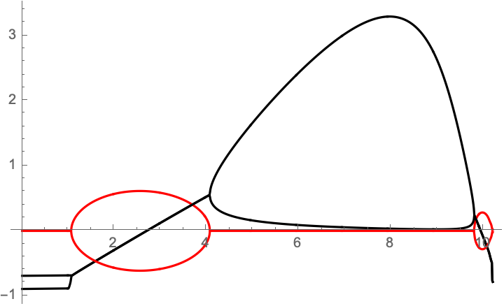
Figure 1. Eigenvalues.

Our second results is a proof of the supercritical Hopf bifurcation at $b\simeq 2.7$ and of the existence of a branch of periodic solutions emanating from it.

Theorem 2.

At $b=b_{0}=2.6992\ldots$ a Hopf bifurcation occurs. More precisely, for all $b\in[b_{0},b_{1}]$ with $b_{1}=2.7418...$ there exists a periodic solution $(\tilde{U}_{b},\tilde{V}_{b})$, with $\partial\tilde{U}_{b}/\partial t\neq 0$ for all $b>b_{0}$, and $(\tilde{U}_{b_{0}},\tilde{V}_{b_{0}})=(U_{b_{0}},V_{b_{0}})$, where $(U_{b_{0}},V_{b_{0}})$ is the solution obtained in Theorem 1. Furthermore, the map $b\mapsto(\tilde{U}_{b},\tilde{V}_{b})$ is analytic and the minimal period of the solutions varies in the interval $[10.35\ldots,10.97\ldots]$.

The proof of the existence of the branch of periodic solutions is carried out only in the interval $[b_{0},b_{1}]$ because it would be very computationally expensive to consider a wider interval. As it turns out, the solution varies significantly and the size of the domain of analyticity decreases very fast with increasing $b$, which in turn means that a very large number of Fourier coefficients need to be taken into account. Still, there is no theoretical obstruction to the extension of the branch. For illustration purposes, we also proved the existence of a periodic solution at $b=3$:

Theorem 3.

At $b=3$ equation (1) admits an analytic periodic solution $(\tilde{U}_{3},\tilde{V}_{3})$ of period $T=22.91\ldots$.

Note that, when $b$ increases from $2.69\ldots$ to $3$, the period of the solution doubles and the graph of the solution changes dramatically. Figure 2 shows some snapshots of the solution $(\tilde{U}_{3},\tilde{V}_{3})$, while Figure 3 shows the stationary solution $(U_{3},V_{3})$ and the graph of $(\tilde{U}_{3}(\pi/2,t),\tilde{V}_{3}(\pi/2,t))$.

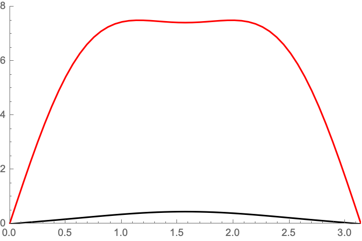
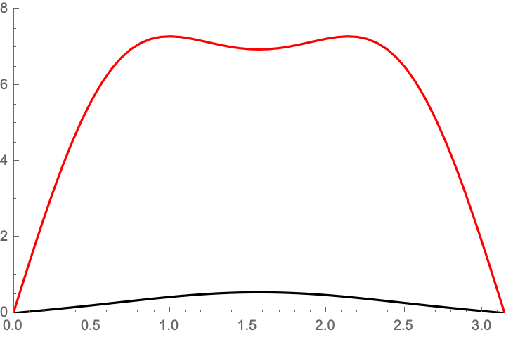
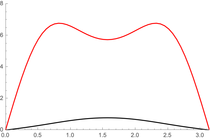
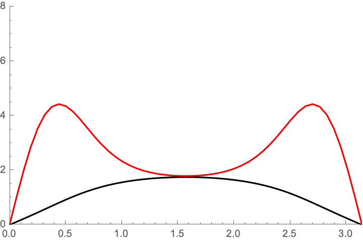
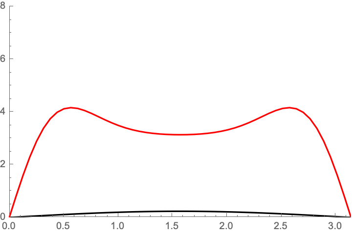
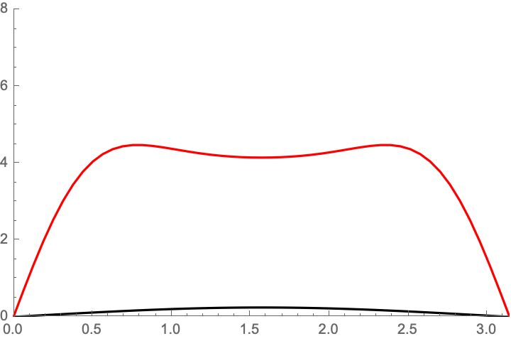
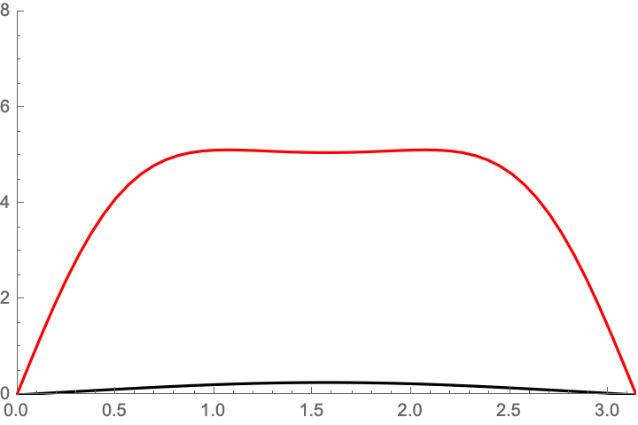
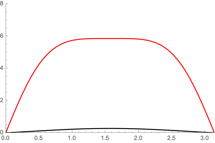
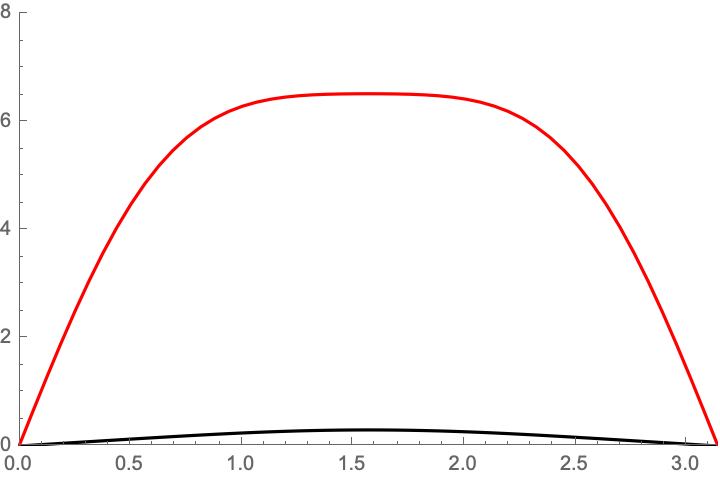
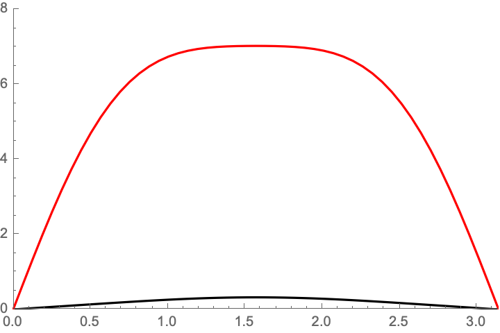
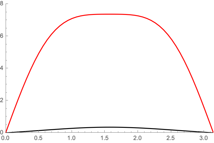
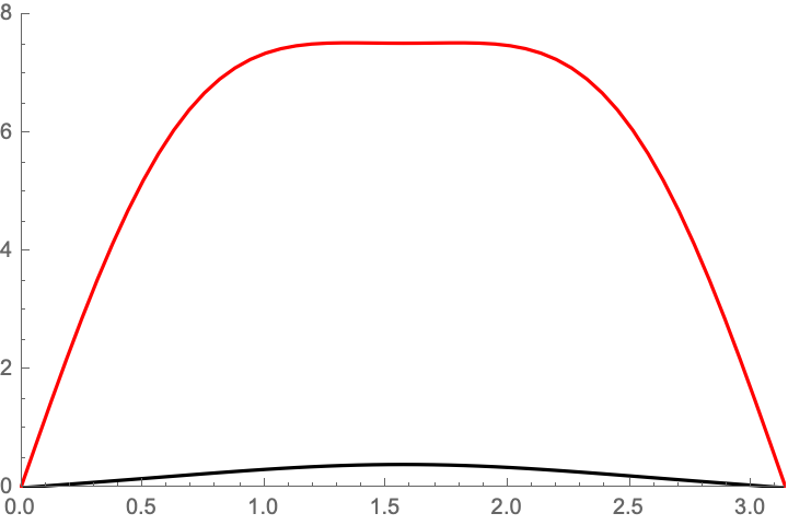
Figure 2. Snapshots of the periodic solutions at $b=3$ at times $t=kT/12$, $k=0,\ldots,11$. The graph of $u$ is black and the graph of $v$ is red.

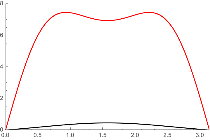
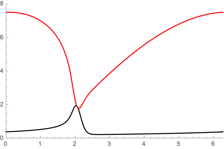
Figure 3. Stationary solution at $b=3$ (left). Graph of $(\tilde{U}_{3}(\pi/2,t),\tilde{V}_{3}(\pi/2,t))$ (right).

2. The strategy of the proofs

2.1. Stationary branch

Let $\rho=65/64$, let $\mathcal{C}$ be the space of functions

(2) $$f=\sum_{k\geq 1}f_{k}\sin(kx)\qquad(f_{k}\in\mathbb{C})$$

such that

(3) $$\|f\|:=\sum_{k}|f_{k}|\rho^{k}<+\infty\,.$$

Denote by $\mathcal{C}_{S}$ the subspace of $\mathcal{C}$ characterized by the symmetry $f(x)=f(\pi-x)$, that is the subspace of functions with $f_{2k}=0$ for all $k=1,2,\ldots$. For $u=(U,V)\in\mathcal{C}^{2}$ let $\|u\|=\|U\|+\|V\|$. Let $A_{b}:\mathcal{C}^{2}\to\mathcal{C}^{2}$ be defined by

(4) $$A_{b}(U,V):=(\partial_{xx})^{-1}(\sin x-(b+1)U+U^{2}V,64(bU-U^{2}V))\,,$$

Clearly, fixed points of $A_{b}$ are analytic stationary solutions of (1). Also note that $A_{b}(U,V)\in\mathcal{C}_{S}^{2}$ for all $(U,V)\in\mathcal{C}_{S}^{2}$.

To prove that $A_{b}$ admits a fixed point $(U_{b},V_{b})\in\mathcal{C}_{S}^{2}$ for each $b\in[0,11]$, and that the function $b\mapsto(U_{b},V_{b})$ is analytic, we write all the coefficients in the Fourier expansion of $(U_{b},V_{b})$ as Taylor polynomials in $b$:

(5) $$(U_{b}(x),V_{b}(x))=\sum_{k\text{ odd}}(u_{k}(b),v_{k}(b))\sin(kx)\,,$$

(6) $$(u_{k}(b),v_{k}(b))=\sum_{l=0}^{L}(u_{kl}(b),v_{kl}(b))\left(b-b_{0}\over b_{1}\right)^{l}\,,$$

where $b_{0},b_{1}$ and $L$ are as in Table 1. As a first step, we choose some Fourier-Taylor polynomial $\bar{u}=(\bar{U},\bar{V})\in\mathcal{C}_{S}^{2}$ that is an approximate fixed point of $A_{b}$, and some finite rank operator $M_{b}:\mathcal{C}^{2}\to\mathcal{C}_{S}^{2}$ such that ${\mathbb{I}}-M_{b}$ is an approximate inverse of ${\mathbb{I}}-DA_{b}(\bar{u})$. Then for $h\in\mathcal{C}^{2}$ we define

(7) $$\mathcal{M}_{b}(h)=A_{b}(\bar{u}+\Lambda_{b}h)-\bar{u}+M_{b}h\,,\qquad\Lambda_{b}={\mathbb{I}}-M_{b}\,.$$

Clearly, if $h$ is a fixed point of $\mathcal{M}_{b}$, then $u=\bar{u}+\Lambda_{b}h$ is a fixed point of $A_{b}$ and, hence, $u$ solves (1). Given $r>0$ and $w\in\mathcal{C}^{2}$, let $B_{r}(w)=\{v\in\mathcal{C}^{2}\,:\,\|v-w\|<r\}$. We partition the interval $[0,11]$ into four subintervals. The center $b_{0}$ and width $b_{1}$ for each subinterval are shown in Table 1.

$i$	$b_{0}$	$b_{1}$	$L$
1	4	4	36
2	17/2	1/2	20
3	19/2	1/2	30
4	21/2	1/2	30

Table 1. Branch intervals for the stationary solution

Then we prove the following lemma with the aid of a computer, see Section 3.

Lemma 1.

The following holds for each $i\in\{1,\ldots,6\}$. Define $b_{0}$, $b_{1}$, and $L$ as in row $i$ of Table 1. There exist a Fourier-Taylor polynomial $\bar{u}(b)$ of degree $L$ as described in (6), a bounded linear operator $M_{b}$ on $\mathcal{C}$, and positive real numbers ${\varepsilon},r,K$ satisfying ${\varepsilon}+Kr<r$, such that

(8) $$\|\mathcal{M}_{b}(0)\|\leq{\varepsilon}\,,\quad\|D\mathcal{M}_{b}(v)\|\leq K\,,\quad\forall v\in B_{r}(0)$$

holds for all $\{b\in\mathbb{C}:|b-b_{0}|<b_{1}\}$. Furthermore,

$$B_{r^{1}}(\bar{u}(b_{0}^{1}+b_{1}^{1}))\subset B_{r^{2}}(\bar{u}(b_{0}^{2}-b_{1}^{2}))\,,$$

$$B_{r^{3}}(\bar{u}(b_{0}^{3}+b_{1}^{3}))\subset B_{r^{4}}(\bar{u}(b_{0}^{4}-b_{1}^{4}))\,,$$

$$B_{r^{3}}(\bar{u}(b_{0}^{3}-b_{1}^{3}))\subset B_{r^{2}}(\bar{u}(b_{0}^{2}+b_{1}^{2}))\,,$$

where the superscript refers row in Table 1.

This lemma, together with the Contraction Mapping Theorem and the Implicit Function Theorem, implies Theorem 1.

2.2. Periodic branch

The time period $T$ of a (non stationary) periodic solution varies with $b$. Instead of looking for $T$-periodic solutions of equation (1), we look for $2\pi$-periodic solutions of

(9) $$\begin{cases}\alpha U_{t}-U_{xx}=\sin x-(b+1)U+U^{2}V\\ \alpha V_{t}-\frac{1}{64}V_{xx}=bU-U^{2}V\\ U(0,t)=U(\pi,t)=V(0,t)=V(\pi,t)=0\quad\forall t\,,\end{cases}$$

where $\alpha=2\pi/T$ has to be determined. To simplify notation, a $2\pi$-periodic function will be identified with a function on the circle $\mathbb{R}/(2\pi\mathbb{Z})$.

Let $\rho=33/32$ and $\varrho=1+2^{-20}$, let

$$\mathop{\rm cosi}\nolimits_{j}(t)=\begin{cases}\cos(jt)&\text{ if }j\geq 0\\ \sin(-jt)&\text{ if }j<0\,,\end{cases}$$

and let ${\mathcal{A}}$ be the space of functions

$$f(t)=\sum_{j\in\mathbb{Z}}f_{j}\mathop{\rm cosi}\nolimits_{j}(t)\,,$$

with

$$\|f\|=\sum_{j\in\mathbb{Z}}|f_{j}|\varrho^{|j|}<+\infty\,.$$

Given $f\in{\mathcal{A}}$, let

$$f_{\rm e}\displaystyle\mathrel{\mathop{=}^{\scriptscriptstyle\rm def}}\sum_{j\text{ even}}f_{j}\mathop{\rm cosi}\nolimits_{j}(t)\,,\qquad f_{\rm o}\displaystyle\mathrel{\mathop{=}^{\scriptscriptstyle\rm def}}\sum_{j\text{ odd}}f_{j}\mathop{\rm cosi}\nolimits_{j}(t)\,.$$

Let ${\mathcal{B}}$ be the space of functions

$$(U(x,t),V(x,t))=\sum_{k\geq 1}(U_{k}(t),V_{k}(t))\sin(kx)\,,\\$$

with $U_{k},V_{k}\in{\mathcal{A}}$ and

$$\|(U,V)\|=\sum_{k\geq 1}(\|U_{k}\|+\|V_{k}\|)\rho^{k}<+\infty\,.$$

Given $(U,V)\in{\mathcal{B}}$, let

$$(U_{\rm o},V_{\rm o})\displaystyle\mathrel{\mathop{=}^{\scriptscriptstyle\rm def}}\sum_{k\geq 1}(U_{k{\rm o}}(t),V_{k{\rm o}}(t))\sin(kx)\,,$$

and define $(U_{\rm e},V_{\rm e})$ similarly. For $b$ near the bifurcation point $b_{0}$, we expect $U,V$ to be nearly time-independent. So in particular, $(U_{\rm o},V_{\rm o})$ is close to zero. This justifies the following scaling: for some $\beta>0$ define

$$(U,V)=T_{\beta}(u,v)\displaystyle\mathrel{\mathop{=}^{\scriptscriptstyle\rm def}}(u_{\rm e}+\beta u_{\rm o},v_{\rm e}+\beta v_{\rm o})\,.$$

Substituting into (1) yields the equation

(10) $$\begin{cases}\alpha u_{t}-d_{1}u_{xx}=\sin x-(b+1)u+{\mathcal{N}}_{s}(u,v)\\ \alpha v_{t}-d_{2}v_{xx}=bu-{\mathcal{N}}_{s}(u,v)\,.\end{cases}$$

where $s=\beta^{2}$ and

(11) $${\mathcal{N}}_{s}(u,v)=u_{e}^{2}v_{e}+2u_{e}u_{o}v_{e}+u_{e}^{2}v_{o}+s(u_{o}^{2}v_{e}+2u_{e}u_{o}v_{o}+u_{o}^{2}v_{o})\,.$$

Let

$${\mathcal{L}}_{\alpha,d,b}u\displaystyle\mathrel{\mathop{=}^{\scriptscriptstyle\rm def}}(\alpha\partial_{t}-d\partial_{xx}+b)^{-1}u\,.$$

Then, if

$$u(x,t)=\sum_{j,k}u_{jk}\mathop{\rm cosi}\nolimits_{j}(t)\sin{kx}$$

we have

(12) $${\mathcal{L}}_{\alpha,d,b}u(x,t)=\sum_{k\geq 1,j\in\mathbb{Z}}\frac{(dk^{2}+b)u_{jk}-\alpha ju_{(-j)k}}{(dk^{2}+b)^{2}+\alpha^{2}j^{2}}\sin(kx)\mathop{\rm cosi}\nolimits_{j}(t)\,,$$

and (1) is equivalent to

(13) $$\begin{cases}u={\mathbb{F}}_{s}(u,v):={\mathcal{L}}_{\alpha,d_{1},b+1}(\sin x+{\mathcal{N}}_{s}(u,v))\\ v={\mathbb{G}}_{s}(u,v):={\mathcal{L}}_{\alpha,d_{2},0}(bu-{\mathcal{N}}_{s}(u,v))\,.\end{cases}$$

One of the features of the equation is that the time-translate of a solution is again a solution. We eliminate this symmetry by imposing the condition $u_{11}=0$. In addition, close to the Hopf bifurcation point, we normalize the odd part of $u$ by choosing $u_{(-1)1}=1$. This leads to the conditions

(14) $$Au\displaystyle\mathrel{\mathop{=}^{\scriptscriptstyle\rm def}}u_{11}=0\,,\qquad Bu\displaystyle\mathrel{\mathop{=}^{\scriptscriptstyle\rm def}}u_{(-1)1}=1\,.$$

It is convenient to regard $s$ to be the independent parameter and express $\alpha$ and $b$ as a function of $s$. The functions $\alpha=\alpha(s)$ and $b=b(s)$ are determined by the condition that $u$ satisfies (14). Applying $A$ and $B$ to both sides of $u={\mathbb{F}}_{s}(u,v)$, and using the identities $A\partial_{xx}=-A$, $A\partial_{t}=B$, $B\partial_{xx}=-B$, $B\partial_{t}=-A$, we find that

(15) $$\alpha=A{\mathcal{N}}_{s}(u,v)\,,\qquad b=B{\mathcal{N}}_{s}(u,v)-1-d_{1}\,.$$

To compute the derivatives of $\{{\mathbb{F}}_{s},{\mathbb{G}}_{s}\}$, assume that $u,v$ depend on a parameter, and denote by a dot the derivative with respect to this parameter. Define

$${\mathcal{L}}_{\alpha,d,b}^{\prime}=\partial_{t}(\alpha\partial_{t}-d\Delta+b)^{-1}\,.$$

Then the parameter-derivatives of ${\mathbb{F}}_{s}(u,v)$ and ${\mathbb{G}}_{s}(u,v),$ are given by

$$D{\mathbb{F}}_{s}(u,v)[\dot{u},\dot{v}] ={\mathcal{L}}_{\alpha,d,b+1}(D{\mathcal{N}}_{s}(u,v)[\dot{u},\dot{v}]-\dot{\alpha}{\mathcal{L}}_{\alpha,d,b+1}^{\prime}(\sin x+{\mathcal{N}}_{s}(u,v))$$

$$-\dot{b}{\mathcal{L}}_{\alpha,d,b+1}(\sin x+{\mathcal{N}}_{s}(u,v)))\,,$$

$$D{\mathbb{G}}_{s}(u,v)[\dot{u},\dot{v}] ={\mathcal{L}}_{\alpha,d,0}(\dot{b}u+b\dot{u}-D{\mathcal{N}}_{s}(u,v)[\dot{u},\dot{v}]$$

$$-\dot{\alpha}{\mathcal{L}}_{\alpha,d,0}^{\prime}(bu-{\mathcal{N}}_{s}(u,v)))\,,$$

where

$$\dot{\alpha}=AD{\mathcal{N}}_{s}(u,v)[\dot{u},\dot{v}]\text{ and }\dot{b}=BD{\mathcal{N}}_{s}(u,v)[\dot{u},\dot{v}]\,.$$

Away from the Hopf bifurcation point there is no need to normalize the odd part of $u$, so that $b$ can be a free parameter and then we choose $\beta=1$. In this case, imposing the condition $Aw=0$ we find that

$$\alpha=\frac{A{\mathcal{N}}_{1}(u,v)}{Bu}\,,$$

and the parameter-derivatives of ${\mathbb{F}}_{1}(u,v)$ and ${\mathbb{G}}_{1}(u,v),$ are given by

$$D{\mathbb{F}}_{1}(u,v)[\dot{u},\dot{v}] ={\mathcal{L}}_{\alpha,d,b+1}(D{\mathcal{N}}_{1}(u,v)[\dot{u},\dot{v}]-\dot{\alpha}{\mathcal{L}}_{\alpha,d,b+1}^{\prime}(\sin x+{\mathcal{N}}_{1}(u,v)))\,,$$

$$D{\mathbb{G}}_{1}(u,v)[\dot{u},\dot{v}] ={\mathcal{L}}_{\alpha,d,0}(b\dot{u}-D{\mathcal{N}}_{1}(u,v)[\dot{u},\dot{v}]-\dot{\alpha}{\mathcal{L}}_{\alpha,d,0}^{\prime}(bu-{\mathcal{N}}_{1}(u,v)))\,.$$

To prove that (1) admits a periodic solution $(U_{b},V_{b})\in\mathcal{C}_{S}^{2}$ for each $b\in[b_{0},b_{1}]$, and that the function $b\mapsto(U_{b},V_{b})$ is analytic, we follow a procedure similar to the stationary case: we write all the coefficients in the Fourier expansion of $(u,v)$ as Taylor polynomials in $s$:

(16) $$(u_{jk}(s),v_{jk}(s))=\sum_{l=0}^{L}(u_{jkl},v_{jkl})\left(s-s_{0}\over\delta\right)^{l}\,.$$

Let

$${\mathbb{H}}_{s}(u,v)\displaystyle\mathrel{\mathop{=}^{\scriptscriptstyle\rm def}}({\mathbb{F}}_{s}(u,v),{\mathbb{G}}_{s}(u,v))\,,$$

so that periodic solutions of (1) correspond to fixed points of ${\mathbb{H}}_{s}$. Let ${\mathcal{B}}_{S}\displaystyle\mathrel{\mathop{=}^{\scriptscriptstyle\rm def}}\{(u,v)\in{\mathcal{B}}\,:\,u(x,t)=u(\pi-x,t)\,,v(x,t)=v(\pi-x,t)\}$, and note that ${\mathbb{H}}_{s}(u,v)\in{\mathcal{B}}_{S}$ for all $(u,v)\in{\mathcal{B}}_{S}$.

As a first step, we choose some Fourier-Taylor polynomial $\bar{w}=(\bar{u},\bar{v})\in{\mathcal{B}}_{S}$, that is an approximate fixed point of ${\mathbb{H}}_{s}$, and some finite rank operator $M=M(s)$ such that ${\mathbb{I}}-M$ is an approximate inverse of ${\mathbb{I}}-D{\mathbb{H}}_{s}(\bar{w})$ and $Mw\in{\mathcal{B}}_{S}$ for all $w\in{\mathcal{B}}_{S}$. Then for $h\in{\mathcal{B}}_{S}$ we define

(17) $${\mathcal{N}}_{s}(h)={\mathbb{H}}_{s}(\bar{w}+\Lambda h)-\bar{w}+Mh\,,\qquad\Lambda={\mathbb{I}}-M\,.$$

Clearly, if $h$ is a fixed point of ${\mathcal{N}}_{s}$, then $u=\bar{u}+\Lambda h\in{\mathcal{B}}_{S}$ is a fixed point of ${\mathbb{H}}_{s}$ and, hence, $u$ solves (1). Given $r>0$ and $w\in{\mathcal{B}}_{S}$, let $B_{r}(w)=\{v\in{\mathcal{B}}_{S}\,:\,\|v-w\|<r\}$. Lemmas 2 and 3 are proved with the aid of a computer, see Section 3.

Lemma 2.

The following holds for each $i\in\{0,\ldots,5\}$. Let $s_{0i}=i2^{-10}$, $\delta=2^{-11}$. There exist a Fourier-Taylor polynomial $\bar{w}_{i}(s)$ of degree $5$ as described in (6), a bounded linear operator $M_{i}(s)$ on $\mathcal{C}_{S}$, and positive real numbers ${\varepsilon}_{i},r_{i},K_{i}$ satisfying ${\varepsilon}_{i}+K_{i}r_{i}<r_{i}$, such that

(18) $$\|{\mathcal{N}}_{\beta}(0)\|\leq{\varepsilon}_{i}\,,\quad\|D{\mathcal{N}}_{\beta}(w)\|\leq K_{i}\,,\quad\forall w\in B_{r_{i}}(0)$$

holds for all $\{s\in\mathbb{C}:|s-s_{0i}|<\delta\}$.

Let $I$ be the natural embedding of $\mathcal{C}^{2}_{S}$ into ${\mathcal{B}}_{S}$.

Lemma 3.

$b(0)=2.6992\ldots$ and $b(11\cdot 2^{11})=2.7418\ldots$ (see (15)). For each $i\in\{0,\ldots,4\}$

$$B_{r_{i}}(\bar{w}(s_{0i}+\delta))\subset B_{r^{i+1}}(w(s_{0(i+1)}-\delta))\,,$$

$$B_{r_{0}}(\bar{w}(s_{0}))\subset B_{r}(I(\bar{u}(b(0))))\,.$$

These lemmas, together with the Contraction Mapping Theorem, imply the following proposition, which in turn yields Theorem 2.

Proposition 1.

For each $s\in[0,11\cdot 2^{-11}]$ there exists a fixed point $u_{s}$ of ${\mathbb{H}}_{s}$, $\partial_{t}u_{s}\neq 0$ for all $s>0$, and the curve $s\mapsto u_{s}$ is analytic. Furthermore, $u_{0}$ coincides with the solution $\bar{u}(b(0))$ of Lemma 1.

Finally, Theorem 3 follows from the following Lemma, also proved with computer assistance:

Lemma 4.

Let $b=3$. There exist a polynomial $\bar{w}\in{\mathcal{B}}_{S}$ a bounded linear operator $M$ on ${\mathcal{B}}_{S}$, and positive real numbers ${\varepsilon},r,K$ satisfying ${\varepsilon}+Kr<r$, such that

(19) $$\|{\mathcal{N}}_{1}(0)\|\leq{\varepsilon}\,,\quad\|D{\mathcal{N}}_{1}(w)\|\leq K\,,\quad\forall w\in B_{r}(0)$$

holds for all $\{s\in\mathbb{C}:|s-s_{0i}|<\delta\}$.

3. Technicalities

3.1. Estimates on the linear operators $\boldmath{\mathcal{L}}_{\alpha,d,b}$ and $\boldmath{\mathcal{L}}_{\alpha,d,b}^{\prime}$

Consider the linear operators ${\mathcal{L}}_{\alpha,d,b}$ and ${\mathcal{L}}_{\alpha,d,b}^{\prime}$, with $\alpha,d,b\in\mathbb{R}$. Let $\tilde{u}={\mathcal{L}}_{\alpha,d,b}u$. Using (12) and the Cauchy-Schwarz inequality in $\mathbb{R}^{2}$ we have the estimate

(20) $$|\tilde{u}_{j,k}|\leq C_{j,k}\sqrt{|u_{j,k}|^{2}+|u_{j,-k}|^{2}}\,,\qquad C_{j,k}=\frac{1}{\sqrt{(dj^{2}+b)^{2}+\alpha^{2}k^{2}}}\,.$$

Note that $C_{j,k}$ is a decreasing function of $j,k$ and can be used to estimate ${\mathcal{L}}_{\alpha,d,b}u$ when $u$ is the tail of a Fourier series.

For the operator ${\mathcal{L}}_{\alpha,d,b}^{\prime}$ we have

$$\tilde{u}_{jk}=k\frac{(dj^{2}+b)u_{jk}-\alpha ku_{j(-k)}}{(dj^{2}+b)^{2}+\alpha^{2}k^{2}}\,,\qquad\tilde{u}={\mathcal{L}}^{\prime}_{\alpha,d,b}u\,.$$

A bound analogous to (20) holds, with with

$$C^{\prime}_{j,k}=\frac{|k|}{\sqrt{(dj^{2}+b)^{2}+\alpha^{2}k^{2}}}\leq\frac{1}{\alpha}\,.$$

3.2. The computer assisted part of the proof

The methods used here can be considered perturbation theory: given an approximate solution, prove bounds that guarantee the existence of a true solution nearby. But the approximate solutions needed here are too complex to be described without the aid of a computer, and the number of estimates involved is far too large.

The first part (finding approximate solutions) is a strictly numerical computation. The rigorous part is still numerical, but instead of truncating series and ignoring rounding errors, it produces guaranteed enclosures at every step along the computation. This part of the proof is written in the programming language Ada [14]. The following is meant to be a rough guide for the reader who wishes to check the correctness of our programs. The complete details can be found in [15].

In the present context, a “bound” on a map $f:{\mathcal{X}}\to{\mathcal{Y}}$ is a function $F$ that assigns to a set $X\subset{\mathcal{X}}$ of a given type (Xtype) a set $Y\subset{\mathcal{Y}}$ of a given type (Ytype), in such a way that $y=f(x)$ belongs to $Y$ for all $x\in X$. In Ada, such a bound $F$ can be implemented by defining a procedure F(X :  in Xtype ;  Y :  out Ytype).

To represent balls in a real Banach algebra ${\mathcal{X}}$ with unit ${\bf 1}$ we use pairs S=(S.C,S.R), where S.C is a representable number (Rep) and S.R a nonnegative representable number (Radius). The corresponding ball in ${\mathcal{X}}$ is $\langle{\tt S},{\mathcal{X}}\rangle=\{x\in{\mathcal{X}}:\|x-({\tt S.C}){\bf 1}\|\leq{\tt S.R}\}$.

When ${\mathcal{X}}=\mathbb{R}$ the data type described above is called Ball. Our bounds on some standard functions involving the type Ball are defined in the packages Flts_Std_Balls. Other basic functions are covered in the packages Vectors and Matrices. Bounds of this type have been used in many computer-assisted proofs; so we focus here on the more problem-specific aspects of our programs.

The computation and validation of branches involves Taylor series in one variable, which are represented by the type Taylor1 with coefficients of type Ball. The definition of the type and its basic procedures are in the package Taylors1. Given a Radius $\rho$, consider the space $\mathbb{T}_{\rho}$ of all real analytic functions $g(t)=\sum_{n}g_{n}t^{n}$ on the interval $|t|<\rho$, obtained by completing the space of polynomials with respect to the norm $\|g\|_{\rho}=\sum_{n}|g_{n}|\rho^{n}$. Given a positive integer D, a Taylor1 is a triple P=(P.C,P.F,P.R), where P.F is a nonnegative integer, ${\tt P.R}=\rho$, and P.C is an array(0..D) of Ball. The corresponding set in $\langle{\tt Taylor1},\mathbb{T}_{\rho}\rangle$ is defined as

(21) $$\langle{\tt P},\mathbb{T}_{\rho}\rangle=\sum_{n=0}^{m-1}\bigl{\langle}{\tt P.C(n)},\mathbb{R}\bigr{\rangle}p_{n}+\sum_{n=m}^{D}\bigl{\langle}{\tt P.C(n)},\mathbb{T}_{\rho}\bigr{\rangle}p_{n}\,,\qquad p_{n}(t)=t^{n}\,,$$

where $m=\min({\tt P.F},{\tt D}+1)$. For the operations that we need in our proof, this type of enclosure allows for simple and efficient bounds.

Consider now the space ${\mathcal{A}}$ for a fixed domain radius $\varrho>1$ of type Radius. Functions in ${\mathcal{A}}$ are represented by the type Fourier1 defined in the package HFouriers1, which accepts coefficients in some Banach algebra with unit ${\mathcal{X}}$. In our application the coefficients of Fourier1 are Taylor1. The type Fourier1 consists of a triple F=(F.C,F.E,F.Freq0), where F.C is an array(-K,0..K) of Ball, F.E is an array(-2*K..2*K) of Radius and F.Freq0 is a boolean flag that, when True, indicates that the object Fourier1 represents a constant function. The corresponding set $\langle{\tt F},{\mathcal{A}}\rangle$ is the set of all function $u=p+h\in{\mathcal{A}}$, where

$$p(t) =\sum_{j=-K}^{K}\langle{\tt F.C(J)},{\mathcal{X}}\rangle\,\mathop{\rm cosi}\nolimits_{j}(t)\,,\qquad h=\sum_{j=-2K}^{2K}h^{j}\,,$$

$$h^{j}(t) =\sum_{m\geq 0}h^{j}_{2m}\,\mathop{\rm cosi}\nolimits_{j+2m}(t)\text{ if }j\geq 0\,,$$

$$h^{j}(t) =\sum_{m\geq 0}h^{j}_{2m}\,\mathop{\rm cosi}\nolimits_{j-2m}(t)\text{ if }j<0$$

with $\|h^{J}\|\leq{\tt F.E(J)}$, for all $J$. Note that high order errors for the even frequencies and odd frequencies are handled separately. For the operations that we need in our proof, this type of enclosure allows for simple and efficient bounds. In particular, note that the nonlinearity in (11) requires a nonstandard product, depending on the parameter $s$. The procedure Prod in the package HFouriers1 provides bounds for that product.

We note that Fourier1 (just like Taylor1) allows a generic type Scalar for its coefficients; and this Scalar can be again a Taylor (or Fourier) series. This feature makes it easy to represent Fourier series whose coefficients depend on parameters.

To represent the space ${\mathcal{B}}$ we use a package Fouriers1 which is very similar to the package HFouriers1, so that we do not provide a detailed description here. The main differences consist in having a standard product, and high order errors for the even frequencies and odd frequencies are handles together.

More precisely, the package Fouriers1 is instantiated with scalars of type Fouriers1 defined in HFouriers1, which in turn has scalars defined in Taylors1. For simplicity, the space $\mathcal{C}$ is represented with the same object, with $K=0$.

A bound on the map ${\mathbb{H}}_{s}$ is implemented by the procedure GMap in the package Taylors1.Foor.Fix. Defining and estimating a contraction like ${\mathcal{N}}_{\beta}$ is a common task in many of our computer-assisted proofs. An implementation is done via two generic packages, Linear and Linear.Contr. For a description of this process we refer to [17].

References

- [1] A. Turing, The chemical basis of morphogenesis, Philos. Trans. Roy. Soc. Ser. B 237 (1952) 37-72.
- [2] M. Al-Ghoul and B.C. Eu, Hyperbolic reaction-diffusion equations, patterns, and phase speeds for the Brusselator, J. Phys. Chemistry, 100 (1996), 18900-18910.
- [3] J.F.G. Auchmuty and G. Nicolis, Bifurcation analysis of nonlinear reaction-diffusion equations - I: Evolution equations and the steady state solutions, Bull. Math. Biology, 37 (1975), 323-365.
- [4] K.J. Brown and F.A. Davidson, Global bifurcation in the Brusselator system, Nonlinear Analysis, 24 (1995), 1713-1725.
- [5] A. Doelman, T.J. Kaper, and P.A. Zegeling, Pattern formation in the one-dimensional Gray-Scott model, Nonlinearity, 10 (1997), 523-563.
- [6] T. Erneux and E. Reiss, Brusselator isolas, SIAM J. Appl. Math., 43 (1983), 1240-1246.
- [7] R.J. Fields and M. Burger, Oscillation and Traveling Waves in Chemical Systems, John Wiley and Sons, 1985.
- [8] P. Gray and S.K. Scott, Sustained oscillations and other exotic patterns of behavior in isothermal reactions, J. Phys. Chemistry, 89 (1985), 22-32.
- [9] P. Gray and S.K. Scott, Chemical Waves and Instabilities, Clarendon, Oxford, 1990.
- [10] T. Kolokolnikov, T. Erneux, and J. Wei, Mesa-type patterns in one-dimensional Brusselator and their stability, Physica D, 214(1) (2006), 63-77.
- [11] J.E. Pearson, Complex patterns in a simple system, Science, 261 (1993), 189-192.
- [12] I. Prigogine and R. Lefever, Symmetry-breaking instabilities in dissipative systems, J. Chem. Physics, 48 (1968), 1665-1700.
- [13] B. Peña and C. Pérez-García, Stability of Turing patterns in the Brusselator model, Phys. Review E, 64(5), 2001.
- [14] Ada Reference Manual, ISO/IEC 8652:2012(E)
- [15] G. Arioli, Programs and data files for the proof of Lemmas 1, 2, and 3, http://www1.mate.polimi.it/~gianni/brus.tgz
- [16] G. Arioli, H. Koch, Computer-Assisted Methods for the Study of Stationary Solutions in Dissipative Systems, Applied to the Kuramoto-Sivashinski Equation Arch. Rational Mech. Anal. 197 (2010) 1033-1051
- [17] G. Arioli, H. Koch, Traveling wave solutions for the FPU chain: a constructive approach, Nonlinearity 33, 1705–1722 (2020)
- [18] M.T. Nakao, Y. Watanabe, N. Yamamoto, T. Nishida, M.-N. Kim, Computer assisted proofs of bifurcating solutions for nonlinear heat convection problems, J. Sci. Comput. 43, 388–401 (2010).
- [19] M.T. Nakao, M. Plum, Y. Watanabe, Numerical verification methods and computer-assisted proofs for partial differential equations, Springer Series in Computational Mathematics, Vol. 53, Springer Singapore, 2019.
- [20] J. Gómez-Serrano, Computer-assisted proofs in PDE: a survey, SeMA 76, 459–484 (2019).
- [21] G. Arioli, F. Gazzola, H. Koch, Uniqueness and bifurcation branches for planar steady Navier-Stokes equations under Navier boundary conditions, in print on J. Math. Fluid Mech.
- [22] G. Arioli, H. Koch, Hopf bifurcation in the planar Navier-Stokes equations, Preprint 2020
- [23] J. B. van den Berg, J.-P. Lessard, E. Queirolo, Rigorous verification of Hopf bifurcations via desingularization and continuation, Preprint 2020
- [24] J. B. van den Berg, E. Queirolo, Validating Hopf bifurcation in the Kuramoto-Sivashinky PDE, Preprint 2020