Radial oscillations and gravitational wave echoes of strange stars with nonvanishing lambda

Abstract

We study the effect of the cosmological constant on radial oscillations and gravitational wave echoes (GWEs) of non-rotating strange stars. To depict strange star configurations we used two forms of equations of state (EoSs), viz., the MIT Bag model EoS and the linear EoS. By taking a range of positive and negative values of cosmological constant, the corresponding mass-radius relationships for these stars have been calculated. For this purpose, first we solved the Tolman-Oppenheimer-Volkoff (TOV) equations with a non-zero cosmological constant and then we solved the pressure and radial perturbation equations arising due to radial oscillations. The eigenfrequencies of the fundamental $f$-mode and first 22 pressure $p$-modes are calculated for each of these EoSs. Again considering the remnant of the GW170817 event as a strange star, the echo frequencies emitted by such stars in presence of the cosmological constant are computed. From these numerical calculations, we have inferred relations between cosmological constant and mode frequency, structural parameters, GWE frequencies of strange stars. Our results show that for strange stars, the effective range of cosmological constant is $10^{-15}\,\mbox{cm}^{-2}\leq\,\Lambda\,\leq 3\times 10^{-13}\,\mbox{cm}^{-2}$.

I Introduction

In 1916 Albert Einstein introduced the term cosmological constant $\Lambda$ as a modification in his field equation to achieve a static, stationary universe, which was believed to be the state of the universe at that time. This new term introduced by him is a dimensionful free parameter carroll . But after the discovery of the redshift of stars and consequently an expanding universe by Hubble this idea of cosmological constant was quickly abandoned. Later, it was reintroduced to overcome the age crisis problem and to construct a universe satisfying the “perfect cosmological principle” bondi ; hoyle . On the contrary, current astrophysical and cosmological observational data reveal that we are in the era of cosmological expansion and the expansion rate of the universe is increasing rather than decreasing riess ; perlmutter . One of the strong beliefs is that the present accelerated expansion of the universe is due to an exotic form of energy known as dark energy. Although it suffers from the fine-tuning problem, $\Lambda$ has been considered as one of the prime candidates of dark energy in the sense that it forms the vacuum energy Peebles . As dark energy pervades throughout the universe, the energy density inside the compact objects should be affected by it, and hence it is necessary to see the effect of dark energy content on the behaviour of such objects. So, if we consider the contribution of cosmological constant $\Lambda$ in compact objects it will be related to the acceleration of the currently observable universe or dark energy. This possibility of non-zero $\Lambda$ and it, as a dominating energy density of the universe, is a fascinating problem in nowadays research.

One of the most intriguing parts of the issue of compact stars is the study of unique strange stars. Since the last decade, the subject of strange stars has attracted much attention from the astrophysicist community. These hypothetical stars are unique in the sense that the structural behaviour of such objects rarely matches with that of other compact objects, like white dwarfs and neutron stars. Due to their unique structural behaviour, the strange stars can be regarded as excellent natural laboratories to study, test, or perhaps constrain different modified theories of gravity under extreme conditions that cannot be reached from the earth-based laboratories. By hypothesis, strange matters are the true ground state of the hadrons and hence they are stable matters Witten1984 . So, it could explain the origin of the huge amount of energy released in superluminous supernovae (100 times brighter than normal supernovae) ofek ; ouyed . Such strange matters are composed of deconfined quark matters, mainly of $u$, $d$, $s$ quarks and a small amount of electrons to maintain charge neutrality aclock ; weber2005 .

Our present study consists of two parts. In the first part, we are seeking correlations between the cosmological constant $\Lambda$ and radial oscillation frequencies of strange stars. From long ago, the light variation in a pulsating star has been used to investigate the physical properties like mass, radius of a star. This indirect approach to understanding the physical properties of a star is known as asteroseismology handler2012 . From the birth to the end of a star, nearly every star undergoes some kind of pulsation. Such asteroseismic behavioural studies of stars are mainly of two types: radial and non-radial. For the case of compact objects like white dwarfs, neutron stars, and strange stars, such radial asteroseismic behaviours are reported earlier in Chandrasekhar1964a ; Chandrasekhar1964b ; Chanmugam1977 ; datta1992 . Here, we stick to our study in the case of radial oscillations only of strange stars.

In the second part of this study, we investigate the effect of $\Lambda$ on the gravitational wave echoes (GWEs) of strange stars. It has been recently suggested that some ultra-compact post-merger objects can emit GWEs pani ; manarelli ; abedi ; urbano . Since strange stars are known to be very compact, we describe strange stars as ultra-compact objects by using stiffer equations of state (EoSs). In the recent detection of gravitational waves (GWs) from the binary neutron star merging event GW170817, the nature of the final massive remnant formed is still not confirmed. We consider it as a strange star and evaluate the corresponding echo frequencies emitted by such stars in presence of the cosmological constant $\Lambda$. The ultra-compact stars are those, whose compactness, $\mbox{C}=\mbox{M}/\mbox{R}$ exceeds $1/3$ urbano . Again to be an eligible candidate to emit echo frequencies, the star must possess a photon sphere. This is the region above the surface of the star at a distance of $\mbox{R}=3\,\mbox{M}$ pani . However, the compactness should not exceed Buchdahl’s limit $\mbox{R}=9/4\,\mbox{M}$. Buchdahl’s limit is the upper limit of compactness of fluid stars which describes the maximum amount of mass that can exist in a sphere before it must undergo the gravitational collapse urbano .

In presence of cosmological constant, compact stars are studied earlier in nayak ; Bordbar ; Largani ; Liu ; arbanil . In the article bohmer , the equations describing small radial oscillations of relativistic stars in presence of a cosmological constant $\Lambda$ were reported. They have also studied the impact of cosmological constant $\Lambda$ on the critical adiabatic index. Again Hossein et al. Sk studied the anisotropic compact stars by considering a variable cosmological constant with a static spherically symmetric spacetime described by Krori-Barua metric kb . A similar study was done by Kalam et al. for the anisotropic compact stars with the de Sitter spacetime kalam . In 2014, O. Zubairi and F. Weber derived the modified stellar structure equations to account for a finite value of the cosmological constant in spherically symmetric mass distributions zubairic1 . In zubairic , such equations are derived for the compact stellar structures such as quark star and neutron stars in presence of the cosmological constant $\Lambda$, and the role of the cosmological constant on stars mass, radius, pressure, and density profiles along with the gravitational redshifts were discussed. For compact stars with an equation of state provided by the quark-meson coupling (QMC) model, such effects of the cosmological constant are discussed in nayak . Recently, for stable relativistic polytropic objects, the effect of the cosmological constant is reported in arbanil . A more detailed analysis of the stability of polytropic spheres in the presence of a cosmological constant can be found in posada . For the general relativistic case with a vanishing cosmological constant, the radial oscillation modes and echo frequencies for strange stars are studied in jb . The present study is the extension of our previous study jb in which we had taken into account the dependence of radial oscillation frequencies and GWE frequencies on different model parameters. This work will focus on the impact of the cosmological constant on radial oscillation modes and echo frequencies of strange stars.

Motivated from the previous works mentioned above, we aim at exploring the effect of the cosmological constant on strange stars’ structural behaviour, radial oscillation, and echo frequencies emitted by them and also to find boundary values of it. Here, we take the strange star as a probe to explore the consequences of a non-vanishing cosmological constant and allow it to vary inside the star. Also, the cosmological constant is taken as a matter distribution source of the star and we show that the compactness of the star varies with the cosmological constant. In turn, it implies that the cosmological constant varies inside such dense stars depending on their compactness. The presence of cosmological constant $\Lambda$ describes well the strange star configurations. In particular, we study the structural change in strange stars due to a non-vanishing cosmological constant, focusing on its effects over the radial oscillations and GWEs of strange stars. Here, we have solved the Einstein field equation for some finite values of cosmological constant $\Lambda$ for spherically symmetric mass distribution. By solving the Tolman-Oppenheimer-Volkoff (TOV) equations we have obtained the mass-radius relationships of strange stars in presence of a non-vanishing cosmological constant. Then we have computed the fundamental $f$- mode and first 22 pressure $p$-mode of radial oscillations, and GWE frequencies emitted by strange stars in two types of EoSs.

We have organized the rest of the paper as follows. In Sec. II the general relativistic formulations including TOV equations and perturbation equations are discussed briefly. In Sec. III the considered EoSs are described along with a brief note on the cosmological constant. The emission of GWEs from an ultra-compact object is discussed in Sec. IV. In Sec. V we have discussed the results that are obtained from this study, which is finally followed by the concluding section, i.e. Sec. VI. Here we follow the natural unit system by considering $c=\hbar=1$ and $G=1$ with the metric convention $(-,\,+,\,+,\,+)$.

II General relativistic formulation

II.1 Equations for stellar structure

In this subsection, we discuss briefly about the strange stars in general relativity (GR) in a spacetime with a cosmological constant, i.e. with $\Lambda\neq 0$. The Einstein’s field equation with the cosmological constant reads,

$$G_{\mu\nu}+\Lambda g_{\mu\nu}=8\pi T_{\mu\nu}.$$ (1)

We consider the strange star as isotropic, stable, and non-rotating mass distribution and the perfect fluid inside the strange star is described by the stress-energy tensor,

$$T_{\mu\nu}=(p+\rho)U_{\mu}U_{\nu}+p\,g_{\mu\nu},$$ (2)

where $p$ is the fluid pressure, $\rho$ is the fluid energy density and $U_{\mu}$ are its four-velocities. The line element for a spherically symmetric mass distribution has the form:

$$ds^{2}=-\,e^{\chi(r)}dt^{2}+e^{\lambda(r)}dr^{2}+r^{2}\,d\theta^{2}+r^{2}\sin^{2}\theta\,d\phi^{2}$$ (3)

with the unknown metric functions $\chi(r)$ and $\lambda(r)$ being dependent on the radial coordinate $r$ only. For the exterior problem the field equation (1) gives,

$$e^{\chi(r)}=e^{-\lambda(r)}=1-\dfrac{2M}{r}-\dfrac{\Lambda r^{2}}{3},$$ (4)

where $M$ is the total mass of the star. Similarly for the interior problem we have,

$$e^{\chi(r)}=e^{-\lambda(r)}=1-\dfrac{2m(r)}{r}-\dfrac{\Lambda r^{2}}{3}.$$ (5)

Here $m(r)$ is the mass function within the radius $r$. On matching the exterior and interior solutions at the surface of the star we get, $m(R)=M$, the total mass of the stellar configuration with $R$ being the radius of the star.

The addition of cosmological constant $\Lambda$ in Einstein’s field equation (1) will change the structure of compact objects. Now solving Einstein’s field equation for the energy-momentum tensor (2) we get the stellar structure equations, known as the TOV equations tolman ; tov with the introduction of cosmological constant zubairic as

$$\dfrac{dm}{dr}=4\pi\rho(r)r^{2},$$ (6)

$$\dfrac{dp}{dr}=-(\rho+p)\dfrac{m+4\pi pr^{3}-\dfrac{\Lambda r^{3}}{3}}{r^{2}\left(1-\dfrac{2m(r)}{r}-\dfrac{\Lambda r^{2}}{3}\right)},$$ (7)

$$\dfrac{d\chi}{dr}=-\dfrac{2}{\rho+p}\dfrac{dp}{dr}.$$ (8)

To find static equilibrium stellar configurations equations (6) - (8) are to be integrated along the radial coordinate $r$ with the initial conditions: $m(r=0)=0$, $p(r=0)=p_{c}$ and $\rho(r=0)=\rho_{c}$. The radius of the star can be determined by using the fact that the pressure vanishes at the surface of the star, i.e. $p(r=R)=0$ (see Fig. 2). These equations for stellar structure can be solved for a given EoS. Solutions of these equations can lead us to know about the stellar mass, radius, pressure, density profile, and the gravitational redshift.

II.2 Radial stability equations

The theory of infinitesimal, adiabatic, radial oscillations and the radial stability of relativistic stars was first derived by S. Chandrasekhar in 1964 (Chandrasekhar1964a, ; Chandrasekhar1964b, ). The solutions of these perturbation equations give information about the eigenfrequencies of radial oscillations. In the presence of cosmological constant $\Lambda$, the radial instability equations were investigated earlier in bohmer ; stuchlik . By introducing two dimensionless parameters $\xi=\Delta r/r$ and $\eta=\Delta p/p$, where $\Delta r$ is the radial perturbation and $\Delta p$ is the corresponding Lagrangian perturbations of the pressure, Bhömer and Harko bohmer presented the radial and pressure perturbation equations as

$$\small{\dfrac{d\xi}{dr}=-\,\dfrac{1}{r}\left(3\xi+\dfrac{\eta}{\gamma}\right)-\dfrac{dp}{dr}\dfrac{\xi}{p+\rho}},$$ (9)

$$\dfrac{d\eta}{dr}=\xi\left[\omega^{2}e^{\lambda-\chi}(1+\dfrac{\rho}{p})r-\dfrac{4}{p}\dfrac{dp}{dr}+\;\dfrac{r}{p\,(\rho+p)}{\left(\dfrac{dp}{dr}\right)}^{2}-e^{\lambda}\left(8\pi-\dfrac{\Lambda}{p}\right)(\rho+p)\,r\right]$$

$$+\,\eta\left[\dfrac{1}{(\rho+p)}\dfrac{dp}{dr}-4\pi(\rho+p)\,r\,e^{\lambda}\right],$$ (10)

where $\gamma=\dfrac{dp}{d\rho}(1+\rho/p)$ is the relativistic adiabatic index.

To study the stability of the stellar object against a small radial perturbation we have to integrate equations (9) and (II.2) from the centre to the boundary along with two boundary conditions: one at the centre and other at the surface of the star. As $r\rightarrow 0$, the coefficient of $1/r$ in equation (9) must vanish to avoid the singularity in the equation. So at the centre of the star we get the boundary condition as

$$3\gamma\xi+\eta=0.$$ (11)

From this condition it can be inferred that $\Delta p=-\,3\gamma p\xi$ at the centre of the star, i.e. $(\Delta p)_{r\,=\,0}=-{(3\gamma p\xi)}_{r\,=\,0}$. Again when $r\rightarrow R$, i.e. at the surface of the star, $p\rightarrow 0$. Thus again to avoid singularity this will eventually require that the coefficient of $1/p$ in the equation (II.2) must vanish at the boundary of the star. Using equation (7) in equation (II.2), it can be found from this requirement that

$$\xi\left[\omega^{2}R\left(\dfrac{M}{R^{2}}-\dfrac{\Lambda R}{3}\right)^{-1}\left(1-\dfrac{2M}{R}-\dfrac{\Lambda R^{2}}{3}\right)^{-1}+R\left(\dfrac{M}{R^{2}}-\dfrac{\Lambda R}{3}\right)\left(1-\dfrac{2M}{R}-\dfrac{\Lambda R^{2}}{3}\right)^{-1}\right]$$

$$+\xi\left[\Lambda R\left(\dfrac{M}{R^{2}}-\dfrac{\Lambda R}{3}\right)^{-1}+4\right]=0.$$ (12)

This boundary condition implies that $\Delta p=\,0$ at the stellar surface, i.e. $(\Delta p)_{r\,=\,R}=0$. These coupled differential equations constitute the Sturm- Liouville type eigenvalue problem. These equations (9) and (II.2) together with the boundary conditions (equations (11), (II.2)) determine the eigenvalues or eigenfrequencies $\omega$ of radial oscillations jb . These equations are solved by using the shooting method as described in panotopoulus . If $\omega$ is real, i.e. $\omega^{2}>0$, the configuration is stable and for $\omega^{2}<0$, the configuration becomes unstable against radial oscillations. Again for the stable fundamental mode ($f$-mode) i.e. for $\omega_{0}^{2}>0$, all other higher-order modes will also be stable.

To find the radial oscillation frequencies we first calculated the quantity $\bar{\omega}=\omega\,t_{0}$, which is dimensionless, and here $t_{0}=1\,\mbox{ms}$. The oscillation frequencies are then calculated by

$$\nu=\dfrac{\overline{\omega}}{2\pi}\;\;\mbox{kHz}.$$ (13)

The obtained frequency $\nu$ is now allowed to take some eigenvalues $\nu_{n}$ and for each values of $\nu_{n}$ we have obtained a specific oscillation mode of the star jb .

III Equations of State and the cosmological constant

Before proceeding to discuss the role of the cosmological constant on strange stars’ oscillation and echo frequencies emitted by them, we wish to add a few comments on our choice of stellar models. It is well known that the macroscopic properties of compact objects, such as mass and radius, depend crucially on the EoSs of ultra-compact matter, which is unfortunately not confirmed clearly to date. In this study, the chosen EoSs are those that (i) should be stiff enough to emit GWE, (ii) the model parameters associated with each EoS lie inside the desired range, and (iii) the mass-radius relations of which are within the accepted limits. To describe the stellar structure, in this present work, we are using two EoSs, viz., the MIT Bag model EoS and the linear EoS as mentioned above.

The MIT Bag model corresponds to a relativistic gas of deconfined quark matter with energy density. This EoS satisfies all necessary criteria for strange matter while retaining an elegant simplicity haensel . It was first used by Witten in 1984 Witten1984 . The form of this equation is

$$p=\dfrac{1}{3}(\rho-4\,B).$$ (14)

In this EoS, the density at the stellar surface is given by $\rho(R)=4\,\mbox{B}$, where $p$ is the isotropic pressure, $\rho$ is the energy density and $B$ is the Bag constant. Instead of taking this usual form (14) of the MIT Bag model EoS we have chosen the stiffer form of this EoS as

$$p=\rho-4\,B$$ (15)

The reason behind doing this is that in EoS of the form (14) the compactness of the stellar structure obtained is not enough to emit GWE frequencies. Making it a stiffer one of the form (15) allows the star to get enough compactness to emit GWE frequencies. As reported in aziz , the acceptable range of Bag constant is $(133.68\,\mbox{MeV})^{4}<\mbox{B}<(222.54\,\mbox{MeV})^{4}$. So in this work we choose B as $(190\,\mbox{MeV})^{4}$, which is well inside the desired range.

Other EoS we have used is the linear EoS of the form:

$$p=b\,(\rho-\rho_{s}),$$ (16)

where $b$ is the linear constant and $\rho_{s}$ is the surface energy density rosinska . This EoS was developed by Dey et al. in 1998 dey . We have chosen the linear constant $b=0.910$ and the corresponding value of the surface energy density $\rho_{s}$ is taken. While choosing the constant value, we have kept in mind the conditions for echoing GWs, which restrict that the compactness should be larger than $1/3$, and also it should respect the causality condition ($b\leq 1$) jb . Our chosen value of $b$ lies under these two restrictions.

The dimensionful parameter $\Lambda$ introduced by Einstein in his field equation has the unit of $\mbox{(length)}^{-2}$. We already have mentioned in Sec. I about the various studies on compact objects in presence of cosmological constants nayak ; Bordbar ; Largani ; Liu ; arbanil . Specifically, we would like to mention here that in Ref. zubairic1 , O. Zubairi and F. Weber obtained that the properties of compact objects in our Universe, where $\Lambda$ is very small (predicted via cosmological observations), do not depend on the cosmological constant. They observed that to yield an observable effect, $\Lambda$ would have to be of the order of nuclear density scales $\sim 10^{-14}\,\mbox{cm}^{-2}$. For neutron stars, a maximum mass of $\sim$ 1.68 $\mbox{M}_{\odot}$ was reported by G.H. Bordbar et al. Bordbar using $\Lambda\sim 10^{-18}\,\mbox{cm}^{-2}$. For the case of white dwarfs, a recent study demands the upper limit on $\Lambda$ as, $\Lambda<3\times 10^{-18}\,\mbox{cm}^{-2}$ Liu . Largani et al. found that for neutron stars to have an observable effect of $\Lambda$ in their structure, the typical values of $\Lambda$ to be $\sim 10^{-12}\,\mbox{cm}^{-2}$Largani . In the article arbanil , the authors reported the stellar configuration of polytropic spheres using $\Lambda$ values within the range of $-10^{-15}\leq\Lambda\leq 10^{-15}\,\mbox{cm}^{-2}$. In bohmer , for a star composed of matter having a density equivalent to nuclear energy density, the upper limit of $\Lambda$ was reported to be less than $3\times 10^{-13}\,\mbox{cm}^{-2}$. Thus, motivated by the search of new equilibrium configurations, corresponding radial oscillations, and also the properties of GWE frequencies of strange stars, in this study we have considered a cosmological constant value larger than the one predicted by cosmological observations planck . We have chosen a set of positive and negative values of $\Lambda$ to see its impact on radial oscillation modes and echo frequencies of strange stars. Our chosen values of $\Lambda$ are in multiples of the $\epsilon$ as $-\,150\,\epsilon$, $-\,100\,\epsilon$, $-\,50\,\epsilon$, $5\,\epsilon$, $10\,\epsilon$, and $15\,\epsilon$. These values are in the units of nuclear energy density scale, $\epsilon=140\,\mbox{MeV/\,fm}^{3}$. The study with positive values of cosmological constant $\Lambda$ (which corresponds to de Sitter space) gives a more realistic description of strange stars. These are relevant from the observational point of view and also used in the context of the dark energy model of the universe. Again the negative cosmological constant $\Lambda$ corresponding to anti-de Sitter space is important for anti-de Sitter/conformal field theory correspondence. So this work is a generalized work that is going to contribute significantly in both observational regime and conformal field theory regime. Again, it is worthy to mention that besides the case of the configuration of compact stellar objects, large values of the cosmological constant have been considered in other types of astrophysical situations also arbanil . For instance, in the case of accretion in primordial black holes during the very early universe, the cosmological constant can take values many orders of magnitude greater than that predicted by current observational data zstuch . As described by Carroll in classical GR, there is no preferred choice for the length scale defined by $\Lambda$ carroll . Indeed, the cosmological constant is a measure of the energy density of the vacuum or the state of lowest energy. This value cannot be calculated with any confidence. So, it brings flexibility in choosing scales of various contributions to the cosmological constant carroll .

IV Gravitational wave echoes

As mentioned in Sec. I, an important property of ultra-compact objects is that some of them can emit GWE frequency. It is a very interesting property of such stars. This happens due to the presence of a photon sphere around the surface of the star. More precisely, GWEs originate from the GWs that are trapped between the photon sphere and the surface of the ultra-compact star abedi . As mentioned in abedi , such type of echoes has two natural frequencies: the harmonic or resonance frequencies and the black hole ringdown or quasi-normal mode (QNM) frequencies.

In this study, we have chosen the final remnant of the GW170817 event as a strange star and calculated the GWEs emitted by such ultra-compact objects. The GWE frequency can be approximately estimated from the inverse of the time taken by a massless test particle to travel from the unstable light ring to the centre of the star. This time is the characteristic echo time and can be expressed as urbano

$$\tau_{echo}\equiv\int_{0}^{3M}\!\!\!\!e^{\,(\lambda(r)-\chi(r))/2}\;\mathrm{d}r.$$ (17)

Using the relation for $e^{\,-\lambda(r)}$ from equation (5) in presence of a non-zero cosmological constant $\Lambda$, we can obtain the following expression for characteristic echo time,

$$\tau_{echo}=\int_{0}^{3M}\!\!\!\!\dfrac{1}{\sqrt{e^{\,\chi(r)}\left(1-\dfrac{2m(r)}{r}-\dfrac{\Lambda r^{2}}{3}\right)}}\;\mathrm{d}r.$$ (18)

In this equation, the term $m(r)$ and $\chi(r)$ can be obtained from the solution of TOV equations with non-vanishing cosmological constant $\Lambda$, i.e. of equations (6) - (8). Finally, the characteristic echo frequency can be calculated by using the relation, $\omega_{echo}\approx\pi/\tau_{echo}$.

V Numerical results

     

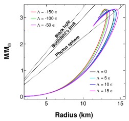
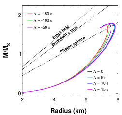
Figure 1: Mass-radius relationships of strange stars for the MIT Bag model EoS (left plot) and linear EoS (right plot) with different cosmological constants showing photon sphere limit, Buchdahl’s limit and black hole limit lines for negative, zero and positive $\Lambda$ values. Mass of stars is expressed in terms of solar mass $\mbox{M}_{\odot}$.

As mentioned earlier, in comparison to other compact objects the structural properties of strange stars are unique. The mass-radius relationship of these stars follows a definite pattern than that of neutron stars. Strange matter can exist in lumps with the size of few fermis to the size of $\sim 10$ km radius strange stars aclock . Using the stiffer MIT Bag model EoS and linear EoS we have plotted the sequences of mass-radius relationships for such stellar configurations. In this study, with the MIT bag model EoS, the maximum mass is obtained as $\approx 3.33\,\mbox{M}_{\odot}$ and the corresponding maximum radius is $\approx 14.34\,\mbox{km}$ and this corresponds to the $\Lambda$ value $15\,\epsilon$. The maximum mass obtained for the linear EoS is $\approx 1.78\,\mbox{M}_{\odot}$ and the maximum radius is $\approx 7.61\,\mbox{km}$ corresponding to the same $\Lambda$ value. The first plot of Fig. 1 shows the relationship for the MIT Bag model EoS and for the linear EoS it is shown in the second plot. As shown in these two plots, for much of these sequences strange stars are following the $\mbox{M}\propto\mbox{R}^{3}$ relation. However, for neutron stars, radii decrease with increasing mass for much of their ranges. For both of the models, with decreasing $\Lambda$, stiffer configurations are obtained. The stiffness is observed to be maximum with $\Lambda=-150\,\epsilon$ and for the MIT Bag model it is higher than the linear EoS. Linear EoSs are giving smaller stellar configurations than the MIT Bag model EoSs. In case, if we choose the general form of the MIT Bag model EoS, then the compactness will not be sufficient to overcome the photon sphere limit as pointed out earlier. The stiffer form of the MIT Bag model and linear EoSs are giving compact enough configurations to cross the photon sphere limit but not Buchdahl’s limit. From Fig. 1, it is clear that the sequences of stellar configurations that are obtained can emit GWE frequencies with the considered $\Lambda$ values.

     

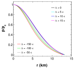
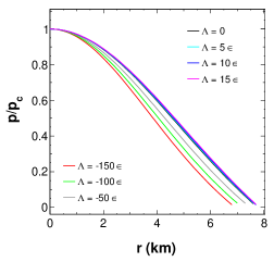
Figure 2: Pressure profiles of strange stars with different $\Lambda$ values for the MIT Bag model EoS (first panel) and the linear EoS (second panel). Here the pressure is scaled in terms of central pressure $p_{c}$.

At this point for the clarity about the physical boundary condition that we have used to calculate the radius of a star as mentioned in section II, we have plotted Fig. 2, which shows the variation of pressure with radial distance $r$ (in km) for different strange star configurations as predicted by the MIT Bag model (left panel) and linear EoS (right panel). These two pressure profiles indicate that pressure near the centre of the star is maximum and it decreases with an increase in the radial distance $r$. Hence, at the surface of the star, the pressure becomes zero as expected.

     

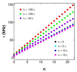
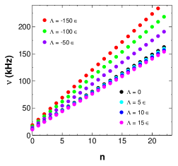
Figure 3: Variation of radial frequencies $\nu_{n}$ with oscillation modes $n$ for different $\Lambda$ values and corresponding to different masses and radii which are listed in Tab. 1. The first plot is for the MIT Bag model EoS and the second plot is for the linear EoS.

As mentioned above, we have calculated the fundamental $f$-mode and 22 lowest $p$-modes of radial oscillation of strange stars for the considered EoSs. The variation of oscillation frequencies $\nu_{n}$ (in kHz) is plotted against the oscillation modes $n$ in Fig. 3. Oscillation frequency increases linearly with the order of modes. For all values of $\Lambda$, it is increasing linearly with increasing modes for both of the EoSs. We have observed the maximum oscillation frequency for $\Lambda=-150\,\epsilon$, and the minimum frequency is obtained for $\Lambda=15\,\epsilon$ for both of the EoSs. The first panel of this figure is for the MIT Bag model EoS and the second panel is for the linear EoS. Linear EoS is giving a frequency above $240\,\mbox{kHz}$, while for the case of the MIT Bag model the maximum frequency is not exceeding $150\,\mbox{kHz}$.

Table 1: Radial oscillation frequencies $\nu_{n}$ in kHz for the MIT Bag model EoS for negative, zero and positive values of $\Lambda$.

Modes (Order n)	$\Lambda=-150\,\epsilon$	$\Lambda=-100\,\epsilon$	$\Lambda=-50\,\epsilon$	$\Lambda=0$	$\Lambda=5\,\epsilon$	$\Lambda=10\,\epsilon$	$\Lambda=15\,\epsilon$
$f$ (0)	10.34	8.76	7.04	5.08	4.85	4.59	4.31
$p_{1}$ (1)	16.07	14.02	11.91	9.88	9.69	9.49	9.30
$p_{2}$ (2)	22.09	19.28	16.52	14.09	13.88	13.68	13.48
$p_{3}$ (3)	28.31	24.67	21.14	18.15	17.91	17.68	17.47
$p_{4}$ (4)	34.59	30.11	25.78	22.16	21.88	21.62	21.38
$p_{5}$ (5)	40.90	35.58	30.43	26.16	25.83	25.52	25.25
$p_{6}$ (6)	47.21	41.06	35.10	30.14	29.76	29.41	29.10
$p_{7}$ (7)	53.53	46.54	39.76	34.13	33.69	33.29	32.94
$p_{8}$ (8)	59.84	52.02	44.43	38.11	37.62	37.17	36.77
$p_{9}$ (9)	66.16	57.05	49.10	42.09	41.55	41.05	40.60
$p_{10}$ (10)	72.47	62.99	53.77	46.07	45.48	44.93	44.43
$p_{11}$ (11)	78.79	68.47	58.45	50.06	49.41	48.81	48.27
$p_{12}$ (12)	85.10	73.95	63.12	54.04	53.34	52.69	52.10
$p_{13}$ (13)	91.41	79.43	67.79	58.03	57.27	56.57	55.93
$p_{14}$ (14)	97.71	84.91	72.47	62.01	61.20	60.44	59.76
$p_{15}$ (15)	104.02	90.37	77.14	66.00	65.13	64.33	63.60
$p_{16}$ (16)	110.33	95.86	81.82	69.99	69.06	68.21	67.43
$p_{17}$ (17)	116.65	101.36	86.49	73.98	72.99	72.09	71.26
$p_{18}$ (18)	122.96	106.77	91.15	77.96	76.93	75.97	75.10
$p_{19}$ (19)	129.28	112.31	95.82	81.95	80.86	79.85	78.93
$p_{20}$ (20)	135.60	117.81	100.50	85.94	84.79	83.74	82.77
$p_{21}$ (21)	141.91	123.33	105.19	89.93	88.73	87.62	86.61
$p_{22}$ (22)	148.23	128.77	109.85	93.92	92.66	91.50	90.44

In Tables 1 and 2, we summarize the radial oscillation frequency modes of strange stars obtained for the MIT Bag model EoS and the linear EoS respectively for all considered values of $\Lambda$. From these tables, it is inferred that for all these modes, more positive $\Lambda$ values are giving smaller oscillation frequencies i.e. with increasing $\Lambda$ values oscillation frequencies are getting smaller for each oscillation mode.

Table 2: Radial oscillation frequencies $\nu_{n}$ in kHz for the linear EoS for negative, zero and positive values of $\Lambda$.

Modes (Order n)	$\Lambda=-150\,\epsilon$	$\Lambda=-100\,\epsilon$	$\Lambda=-50\,\epsilon$	$\Lambda=0$	$\Lambda=5\,\epsilon$	$\Lambda=10\,\epsilon$	$\Lambda=15\,\epsilon$
$f$ (0)	18.67	16.44	14.03	11.44	11.18	10.91	10.64
$p_{1}$ (1)	28.90	25.78	22.42	18.86	18.49	18.13	17.76
$p_{2}$ (2)	38.98	34.90	30.52	25.89	25.41	24.94	24.47
$p_{3}$ (3)	49.06	43.97	38.52	32.79	32.21	31.63	31.05
$p_{4}$ (4)	59.17	53.04	46.50	39.64	38.94	38.25	37.56
$p_{5}$ (5)	69.32	62.12	54.47	46.46	45.65	44.84	44.04
$p_{6}$ (6)	79.51	71.22	62.44	53.27	52.35	51.42	50.50
$p_{7}$ (7)	89.72	80.35	70.42	60.08	59.03	58.00	56.96
$p_{8}$ (8)	99.95	89.49	78.41	66.88	65.72	64.57	63.41
$p_{9}$ (9)	110.21	98.64	86.41	73.69	72.41	71.14	69.87
$p_{10}$ (10)	120.47	107.81	94.42	80.50	79.10	77.71	76.32
$p_{11}$ (11)	130.76	116.98	102.43	87.32	85.80	84.29	82.78
$p_{12}$ (12)	141.05	126.17	110.45	94.13	92.50	90.86	89.24
$p_{13}$ (13)	151.35	135.37	118.48	100.96	99.20	97.44	95.70
$p_{14}$ (14)	161.66	144.57	126.52	107.78	105.91	104.03	102.17
$p_{15}$ (15)	171.97	153.78	134.56	114.61	112.61	110.62	108.63
$p_{16}$ (16)	182.30	162.99	142.60	121.45	119.33	117.21	115.11
$p_{17}$ (17)	192.62	172.21	150.65	128.28	126.04	123.81	121.58
$p_{18}$ (18)	202.95	181.43	158.70	135.12	132.76	130.40	128.06
$p_{19}$ (19)	213.28	190.65	166.76	141.97	139.48	137.00	134.53
$p_{20}$ (20)	223.62	199.88	174.82	148.81	146.20	143.60	141.01
$p_{21}$ (21)	233.96	209.11	182.88	155.66	152.93	150.21	147.50
$p_{22}$ (22)	244.30	218.35	190.94	162.51	159.65	156.81	153.98

Also, each mode frequency for all $\Lambda$ values is larger for the linear EoS than that for the MIT Bag model EoS. These are already visualized in Fig. 3.

     

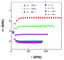
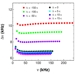
Figure 4: Variation of difference between consecutive modes of radial frequencies ($\Delta\nu_{n}$) with radial frequencies $\nu_{n}$ for different $\Lambda$ values. First panel and second panel are for the MIT Bag model EoS and linear EoS respectively.

In Fig. 4, the variation of separation between two consecutive modes of radial frequencies ($\Delta\nu$) with respect to the mode frequencies $\nu$ is shown. The first panel is for the MIT Bag model and the second panel is for the linear EoS. For the MIT Bag model with positive $\Lambda$ values, a gradually decreasing pattern is observed. The difference between the oscillation frequencies of $f$-mode and $p_{1}$-mode is larger than that of the other values. However, in the case of more negative values of $\Lambda$, the opposite behaviour is observed. Unlike other $\Lambda$ values, for $\Lambda=-150\,\epsilon$ and $-100\,\epsilon$ the difference between oscillation frequencies of $f$-mode and $p_{1}$-mode is smaller than the rest of the variations. In the case of linear EoS, nearly a smooth variation for all the considered $\Lambda$ values is observed. For $\Lambda=-150\,\epsilon$ both EoSs give maximum value of $\Delta\nu$ and for $\Lambda=15\,\epsilon$ they give a minimum value of $\Delta\nu$ in case of modes other than $f$-mode and $p_{1}$-mode with MIT Bag model EoS. That is under this condition $\Delta\nu$ decreases with increasing values of $\Lambda$. This figure also clarifies that for $\Lambda=-150\,\epsilon$, the radial frequencies are maximum whereas the frequencies are minimum for $\Lambda=15\,\epsilon$ for both MIT Bag model EoS and linear EoS as also seen from Tables 1 and 2 respectively.

     

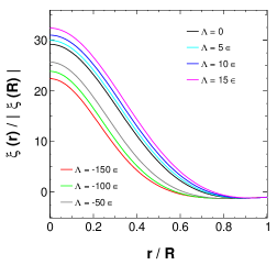
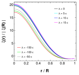
Figure 5: Variation of $f$-mode of radial perturbations $\xi(r)$ with radial distance $r$ (in km) obtained by using the MIT Bag model EoS (first panel) and the linear EoS (second panel) for different $\Lambda$ values.

From the Sturm-Liouville dynamic pulsation equations in presence of a cosmological constant (equations (9)-(II.2)), we have studied the variation of radial and pressure perturbations with the radial distance $r$. In Fig. 5 and 6 the variation of radial perturbation $\xi(r)$ with radial distance $r$ is shown for $f$-mode and $p_{22}$-mode respectively. In the first panel of Fig. 5, the variation of radial perturbation $\xi(r)$ with $r$ (in km) is shown for the MIT Bag model and in the second panel, the variation is shown for the linear EoS. From these two plots, it is clear that the radial perturbation is larger only near the centre of the star. It is diminishing near the surface of the star for both these EoSs. As the EoSs with different $\Lambda$ values are mimicking strange stars of different sizes, the perturbation along the radial distances are found different.

     

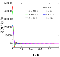
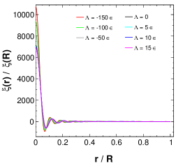
Figure 6: Variation of radial perturbations $\xi(r)$ with radial distance $r$ (in km) obtained by using the MIT Bag model EoS (first panel) and the linear EoS (second panel) for different $\Lambda$ values for the case of pressure $p_{22}$-mode.

Similarly in Fig. 6, the variation is shown for higher-order $p_{22}$-mode. For the MIT Bag model, it is shown in the first panel of the figure. As like the $f$-mode, the perturbation is larger near the centre of the star. Towards the surface, a distinct damping nature of radial perturbation is noticed. The different $\Lambda$ values are also showing distinct variations in their respective perturbations. As shown in the second panel of Fig. 6, for the case of linear EoS, the variation of $p_{22}$ mode is behaving similarly to that of the MIT Bag model EoS. The perturbation is decreasing along the surface of the star. Intermediate pressure perturbations curves can be drawn which will lie in between $f$ and $p_{22}$ modes.

     

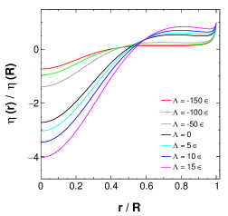
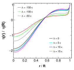
Figure 7: Variation showing pressure perturbations $\eta(r)$ with radial distance $r$ (in km) found by using MIT the Bag model EoS (first panel) and the linear EoS (second panel) for different $\Lambda$ values for fundamental $f$-mode.

The variation of pressure perturbation is different from the variation of radial perturbation. As clear from Fig. 7 and 8, the variation is larger near the centre and surface of each star. Whereas, for the case of radial perturbation, it is larger near the centre of the star only. In the first panel of Fig. 7, the change in pressure perturbation with distance from the centre of the star is showing for the MIT Bag model EoS for fundamental $f$-mode due to different $\Lambda$ values. The different sizes of each star for each $\Lambda$ values are also clear from this plot. Similar behaviour is observed for linear EoS with fundamental $f$-mode. This can be visualised from the second panel of this Fig. 7.These variations shown in this figure correspond to different values of mass and radius corresponding to considered $\Lambda$ values. As an example, for the MIT Bag model EoS i.e. in the left panel of Fig. 7 and for $\Lambda=15\,\epsilon$, the corresponding mass and radius are $\approx 3.3\,\mbox{M}_{\odot}$ and $\approx 14.3\,\mbox{km}$ respectively. The other values of mass and radius corresponding to these variations can be found in Table 3.

     

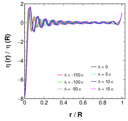
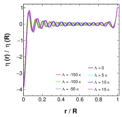
Figure 8: Variation showing pressure perturbations $\eta(r)$ with radial distance $r$ (in km) found by using the MIT Bag model EoS (first panel) and the linear EoS (second panel) for different $\Lambda$ values for the pressure $p_{22}$-mode.

This pressure variation for higher-order oscillation mode i.e. for $p_{22}$-mode is shown in Fig. 8. The first panel corresponds to the MIT Bag model and the second panel corresponds to the linear EoS. Similar to the $f$-mode of oscillation this variation is also larger near the centre and near the surface of the star. For all other modes in between $f$-mode and $p_{22}$-mode, pressure perturbation will stay in between.

     

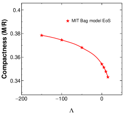
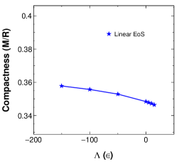
Figure 9: The variation of compactness of strange stars with different $\Lambda$ values for the MIT Bag model EoS (first panel) and the linear EoS (second panel).

The value of cosmological constant $\Lambda$ varying with different strange star configurations can be visualized in Fig. 9. The left panel of this figure is for the MIT Bag model and the right panel is for the linear EoS. For both of the cases, with increasing $\Lambda$ value compactness is found to decrease. The fall is somewhat rapid for the MIT Bag model EoS than that of the linear EoS. The different values of these plots can be found in Table 1 and in Table 2.

     

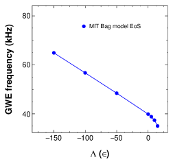
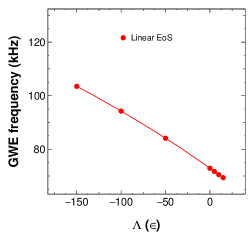
Figure 10: The variation of GWE frequencies with different $\Lambda$ values for the MIT Bag model EoS (first panel) and the linear EoS (second panel).

After the numerical analysis of the perturbation equations, another important part of this work is to find the effect of cosmological constant $\Lambda$ on GWE frequencies. The GWE frequencies are found to diminish with an increase in $\Lambda$ values, for both of the EoSs. For the MIT Bag model with negative $\Lambda$ values the variation is straightaway, however, a rapid drop is observed for positive $\Lambda$ values. The linear EoS is showing almost a straight variation for both positive and negative values of $\Lambda$. These variations are shown in Fig. 10, where the first panel is for the MIT Bag model and the second panel is for the linear EoS.

Table 3: Mass, radius, compactness of strange stars, characteristic echo time and GWEs from strange stars for the MIT Bag model EoS with the bag constant $B=(190\,\mbox{MeV)}^{4}$.

	Value of $\Lambda$	Radius R	Mass M	Compactness	Echo	GWE
(in terms of $\epsilon$)	(in $\,\mbox{cm}^{-2}$)	(in km)	(in $\mbox{M}_{\odot}$)	(M/R)	time (ms)	frequency (kHz)
-150$\,\epsilon$	-2.66$\times 10^{-12}$	13.003	3.327	0.3784	0.048	64.90
-100$\,\epsilon$	-1.77$\times 10^{-12}$	13.090	3.315	0.3745	0.055	56.74
-50$\,\epsilon$	-8.88$\times 10^{-13}$	13.259	3.300	0.3681	0.065	48.44
0	0	13.766	3.295	0.3540	0.078	39.91
5$\,\epsilon$	8.88$\times 10^{-14}$	13.893	3.300	0.3512	0.080	38.86
10$\,\epsilon$	1.77$\times 10^{-13}$	14.067	3.308	0.3477	0.083	37.42
15$\,\epsilon$	2.66$\times 10^{-13}$	14.340	3.326	0.3430	0.089	35.08

Table 4: Mass, radius, compactness of strange stars, characteristic echo time and GWEs from strange stars for the linear EoS with the linear constant $b=0.910$.

	Value of $\Lambda$	Radius R	Mass M	Compactness	Echo	GWE
(in terms of $\epsilon$)	(in $\,\mbox{cm}^{-2}$)	(in km)	(in $\mbox{M}_{\odot}$)	(M/R)	time (ms)	frequency (kHz)
-150$\,\epsilon$	-2.66$\times 10^{-12}$	7.200	1.742	0.3577	0.030	103.42
-100$\,\epsilon$	-1.77$\times 10^{-12}$	7.271	1.749	0.3557	0.033	94.24
-50$\,\epsilon$	-8.88$\times 10^{-13}$	7.372	1.759	0.3529	0.037	84.12
0	0	7.535	1.775	0.3484	0.043	72.91
5$\,\epsilon$	8.88$\times 10^{-14}$	7.558	1.778	0.3478	0.044	71.71
10$\,\epsilon$	1.77$\times 10^{-13}$	7.584	1.780	0.3472	0.045	70.51
15$\,\epsilon$	2.66$\times 10^{-13}$	7.610	1.783	0.3464	0.045	69.40

The properties of stellar structure such as mass, radius, and compactness along with the results for the GWE frequencies and characteristic echo times that are obtained by using the MIT Bag model EoS are compiled in Table 3. From this table, the change in these properties of strange stars for the MIT Bag model with different $\Lambda$ values can be seen clearly. With increasing $\Lambda$ values the size of stars is increasing. The compactness of the stars is decreasing with more positive values. Thus the upper limit on cosmological constant $\Lambda$ value is depicting a star with compactness such that it is just able to echo the falling GWs. For our considered maximum value of $\Lambda$ (15$\,\epsilon$), the compactness is found to be 0.3430, which is greater than 1/3. The characteristic echo time obtained for this EoS increases with the increasing $\Lambda$ value, and hence the reverse effect is noticed for the GWE frequencies. For this EoS, all echo frequencies obtained are in the range of tens of kilohertz.

The sizes of stars obtained by using the linear EoSs are smaller than that obtained for the MIT Bag model EoSs. Eventually, the masses are also small in comparison to that for the MIT Bag model and hence fulfilling the criteria for echoing GWs. These results are shown in Table 4. For all the chosen $\Lambda$ values, the stars are found to be with enough compactness to emit GWE frequencies. The characteristic echo times obtained are smaller than that of the MIT Bag model EoS and hence in turn the larger echo frequencies are obtained for this EoS.

Table 5: Properties of strange stars for the MIT Bag model and linear EoS with different values of $\Lambda$.

	Value of $\Lambda$			MIT Bag model				Linear EoS
(in $\,\mbox{cm}^{-2}$)	(in terms of $\epsilon$)	Radius	Mass	Compactness	Echo freq-	Radius	Mass	Compactness	Echo freq-
		(in km)	(in $\mbox{M}_{\odot}$)	(M/R)	uency (kHz)	(in km)	(in $\mbox{M}_{\odot}$)	(M/R)	uency (kHz)
$1\times 10^{-18}$	5.6$\times 10^{-5}\,\epsilon$	13.766	3.295	0.354	39.91	7.535	1.775	0.348	72.91
$1\times 10^{-16}$	5.6$\times 10^{-3}\,\epsilon$	13.766	3.295	0.354	39.91	7.535	1.775	0.348	72.91
$1\times 10^{-15}$	5.6$\times 10^{-2}\,\epsilon$	13.767	3.296	0.354	39.90	7.535	1.775	0.348	72.89
$1\times 10^{-14}$	5.6$\times 10^{-1}\,\epsilon$	13.778	3.296	0.354	39.80	7.538	1.775	0.348	72.76
$5\times 10^{-14}$	2.8$\,\epsilon$	13.834	3.298	0.353	39.34	7.548	1.776	0.348	72.23
$1\times 10^{-13}$	5.6$\,\epsilon$	13.912	3.301	0.351	38.66	7.558	1.778	0.348	71.71
$2\times 10^{-13}$	11.2$\,\epsilon$	14.122	3.312	0.347	36.99	7.590	1.781	0.347	70.20
$3\times 10^{-13}$	16.8$\,\epsilon$	14.492	3.338	0.341	35.26	7.621	1.784	0.346	68.28

VI Conclusions

In this study, we look into the role of the cosmological constant on two interesting aspects of strange stars. In one part we have tried to understand its impact over the radial oscillations of strange stars and in another, we have investigated its effect on GWE frequencies emitted by a strange star, like the star formed in the binary merging event GW170817. This study is made in the general relativistic framework. To study its role over radial oscillations we solved the TOV equations for two EoSs, viz., the MIT bag model EoS and the linear EoS. The solution of TOV equations leads us to know the structure of strange stars in presence of cosmological constant $\Lambda$, which is found to be different from the structure obtained by using the vanishing $\Lambda$ jb . Again as discussed in Sec. V, different $\Lambda$ values give us different strange star configurations. Moreover, the pulsation equations developed by Chandrasekhar are modified for spacetime with a cosmological constant by introducing two dimensionless parameters $\xi$ and $\eta$. The solution of these pulsation equations gave us eigenfrequencies of oscillations and hence we have calculated the $f$-mode and first 22 $p$-modes of oscillations. We found that the large value of $\Lambda$ decreases the radial oscillation frequencies of stars for both of the EoSs. Further, to see the role of $\Lambda$ on GWEs first we calculated the characteristic echo time of GWs falling on strange stars.

The study clearly shows that at the present cosmological constant value around $\Lambda=(4.24\,\pm\,0.11)\times 10^{-66}\,\mbox{eV}^{2}$ ($\equiv\;\sim 10^{-56}$ cm^-2), the maximum mass and radius, radial oscillations, and echo frequencies of strange stars are identical with the GR values and can’t be distinguished both theoretically and experimentally. Hence, the observations of such parameters of a strange star can’t be used to differentiate between GR and the $\Lambda$CDM model for the present value of $\Lambda$. However, bounds on $\Lambda$ from the stellar stability and interior structure nayak ; Bordbar ; Liu ; arbanil are comparatively weak, which gives us a wide range of possible $\Lambda$ values. We have shown that within this boundary, the cosmological constant $\Lambda$ with a large magnitude can effectively put significant impacts on the mass, radius, radial oscillations, and echo frequencies of a strange star. Our results showed that for strange stars, the effective upper limit of $\Lambda$ is $\sim 3\times 10^{-13}\,\mbox{cm}^{-2}$ and the lower limit is $\sim 10^{-15}\,\mbox{cm}^{-2}$. The maximum mass, radius, radial oscillation frequencies, and echo frequencies of strange star configurations have changed significantly within these boundary values. These impacts again depend on the EoS of the star. These results are presented in Table 5. According to the results of this table the cosmological constant has no significant effect on the properties of a strange star when its value is less than $10^{-15}\,\mbox{cm}^{-2}$. This table generalizes our results, whereas in the graphs only large values of $\Lambda$ are taken to show the changes distinctly and also to visualize the variation pattern or dependency of the same with $\Lambda$ efficiently. Again some Ref.s Bordbar ; Liu ; arbanil ; wei suggest a possibility of varying $\Lambda$ with the cosmological evolution. Similarly, in some modified gravity theories like $f(R)$ gravity in Palatini formalism, the field equations can be written in GR form with an effective $\Lambda$ term pano . This indicates the fact that the cosmological evolution obtained by using a feasible $f(R)$ gravity model can mimic the $\Lambda$CDM model in the present and early universe effectively. However, depending on the functional form and uniqueness of such $f(R)$ models, the effective $\Lambda$ term varies differently dj ; santos . Therefore, consideration of different values of $\Lambda$ in a wide range can be helpful to see the possible impacts of it on the strange star structures in theories with varying dark energy or $f(R)$ gravity in Palatini formalism, where the effective $\Lambda$ term is not a constant. However, we agree that a functional variation of $f(R)$ gravity models can have other impacts on the strange star properties also and we leave it as the future scope of our study. An important outcome of the study is that a $\Lambda$ value below $1\times 10^{-15}\,\mbox{cm}^{-2}$ does not have significant observable impacts on the maximum mass, maximum radius, radial oscillations, and echo frequencies of a strange star with the MIT Bag model and linear EoSs. The boundary values of $\Lambda$ are found to be the same for these two EoSs. As these both EoSs are stiff EoSs, with almost similar compactness so the boundary values on $\Lambda$ are similar for them.

Another important aspect of the study is that the study gives a theoretical idea of the structure of a strange star in terms of a few properties like maximum mass, maximum radius, radial oscillations, and echo frequencies in both de Sitter and anti-de Sitter regime. The study with positive values of cosmological constant $\Lambda$ (which corresponds to de Sitter space) gives a more realistic description of strange stars. These are relevant from the observational point of view and also used in the context of the dark energy model of the universe. On the other hand, the negative cosmological constant $\Lambda$ corresponding to anti-de Sitter space is important for anti-de Sitter/conformal field theory correspondence as mentioned earlier.

To know the enigmatic stellar interior of compact stars using asteroseismology several ground-based missions are proposed in addition to few early space missions in this regard. Some of such important missions are MOST most , CoRoT corot , BRITE brite , Kepler/K2 kepler , PLATO plato , and TESS tess missions. The unplanned pioneer mission in the field of observational asteroseismology was NASA’s WIRE mission wire . The Canadian MOST mission was the first space telescope dedicated to asteroseismology and was proposed to monitor relatively bright stars. The French-led CoRoT mission was a great success for massive star variability studies. The BRITE-constellation of nanosatellites is another important photometry mission available for asteroseismology and it is ranked amongst the highest givers for providing excellent asteroseismic returns. The most famous of all space telescopes providing time series photometry is the Kepler mission launched in 2009. It is targeted to study solar like stars all over the HR diagram. The next generation of stellar missions such as PLATO and other current and future Earth based radio telescopes, such as Arecibo qui or SKA ska have the potential to put important constraints in the stellar properties, or to find such compact stars. Furthermore, the recently launched NASA’s mission NICER nicer , designed primarily to observe thermal X-rays emitted by several millisecond pulsars, is another ray of hope to detect such stars.

Again, the current GW detectors have comparatively low sensitivity (detectable frequency range is $\sim$ 20 Hz - 4 kHz martynov ; abbot ), so unfortunately the ongoing detectors does not allow the detection of such compact stellar oscillation frequencies. The next generation of ground-based GW detectors, e.g., the Einstein Telescope (ET) et and the Cosmic Explorer (CE) ce are expected to have a sensitivity much higher than an order of magnitude in comparison to the Advanced LIGO. These detectors are supposed to detect such emission and provide information on the oscillation of compact stars chiren . If in near future such frequencies are detected, they could also provide the simultaneous measurements of compact star masses, tidal Love numbers benni , frequency, damping time, amplitude of the modes. Furthermore, the expectations for the detection of the compact star’s oscillations will also be increased by the launch of the eXTP extp and other X-ray missions. When the detection of the radial oscillations of neutron stars and other compact stars will become possible, then it can be used to constrain the EoSs of compact stars with high precision and hence the corresponding stellar properties.

From the emission of GWs, the most important modes to be detected are the fundamental $f$-modes and the first few pressure $p$-modes, in addition to the $r$-modes and $w$-modes kokkotas . The $f$-mode of oscillation is the mode through which most of the gravitational radiation of the star is radiated away kokkotas97 . The $p$-mode is associated with the acoustic sound speed inside the star. These $p$- or the low order radial acoustic modes can be observed through the associated GW perturbations. One of the obvious sources of excitation of these radial (or non-radial) acoustic modes is the supernova explosion gpano . The pulsating compact objects formed from such events emit GWs. Strong star-quakes can also arise with their associated pulsar glitches that can excite global stellar pulsations. Again, the compact stars that undergo a phase transition, e.g. when a neutron star collapses into a strange star and the coalescence of two compact stars may form a pulsating remnant compact star lusky . These mechanisms of excitation generally give $f$-modes as well as radial $p$-modes. Moreover, due to the similar excitation mechanism the $f$-modes and $p$-mode can be determined using similar strategy glam . Besides these excitation mechanisms, such modes can also be excited by tidal forces in a close eccentric binary system chirenti and a resonant excitation in binaries hind . Accretion in Low-Mass X-ray Binaries (LMXBs) can also excite these modes ander . Star-quakes caused by cracks in the crust, magnetic reconfiguration or any other dynamical instabilities are also associated with the excitation of stellar oscillation modes franco ; tsang .

It is also worth mentioning that in actual practice, the large amplitude of oscillation modes only occurs in catastrophic situations, such as in core-collapse supernovae. Such events are highly non-spherical and hence in such cases, the non-radial modes could become more applicable. So a possible extension of our present work would be to study the non-radial oscillations of strange stars and the corresponding GW signals associated with them. In abedi , the authors have claimed a tentative detection of echoes from the remnant of GW170817 event at a frequency $\simeq 72\,\mbox{Hz}$. Although the consistent mass ($2.6-2.7\,\mbox{M}_{\odot}$) of this remnant almost lies within the range of masses of strange stars predicted by our EoSs with different $\Lambda$ values, the GWE frequencies found from our calculations are much higher (in kHz range) than this tentative detection value. The basic reason for the difference between this result and our results is that instead of considering the remnant of GW170817 as an exotic compact object (ECO), we have considered the star of this mass range as a strange star. Further, while considering the EoSs, we have neglected the possible temperature effect on EoS. Again we choose strange stars as non-rotating ones and solved the TOV equations for the static stellar model while investigating these properties. So, the study of rotating, anisotropic strange stars or, other possible ECO is a topic that will be considered for future work.

References

- (1) S. M. Carroll Liv. Rev. Rel. 4, 1 (2001).
- (2) H. Bondi and T. Gold, Mon. Not. R. Astron. Soc. 108, 252 (1948).
- (3) F. Hoyle, J. V. Narlikar, P. A. M. Dirac, H. Bondi, R. Schlegel, W. Davidson and J. L. Synge, Proc. R. Soc. London A 270, 334 (1962).
- (4) A. G. Riess et al., Astrophys. J. 116, 1009-1038 (1998), [arXiv:astro-ph/9805201].
- (5) S. Perlmutter et al., Astrophys. J. 517, 565-586 (1999).
- (6) P. J. E. Peebles, B. Ratra, Rev. Mod. Phys. 75 (2003) 559.
- (7) E. Witten, Phys. Rev. D 30, 272 (1984).
- (8) E. O. Ofek et al., Astrophys. J. 659 (2007) L13.
- (9) R. Ouyed, D. Leahy and P. Jaikumar, Compact stars in the QCD phase diagram II (CSQCD II) KIAA at Peking University, Beijing-P. R. China (2009).
- (10) C. Alcock, E. Farhi and A. Olinto, Astrophs. J. 310, 261-272 (1986).
- (11) F. Weber, Prog. Part. and Nucl. Phys. 54, 193 (2005).
- (12) G. Handler, Planets, Stars and Stellar Systems, Springer, (2013) [arXiv:1205.6407] .
- (13) S. Chandrasekhar, Astrophys. J. 140, 417 (1964).
- (14) S. Chandrasekhar, Phys. Rev. Lett. 12, 114 (1964).
- (15) G. Chanmugam, Astrophs. J. 217, 799 (1977).
- (16) B. Datta, P. K. Sahu, J. D. Anand and A. Goyal, Phys. Lett. B 283, 313 (1992).
- (17) P. Pani and V. Ferrari, Class. Quan. Grav. 35, 15LT01 (2018).
- (18) M. Mannarelli and F. Tonelli, Phys. Rev. D 97, 123010 (2018).
- (19) J. Abedi and N. Afshordi, JCAP 11, 010 (2019),.
- (20) A. Urbano and H. Veermäe JCAP 1904 04, 011 (2019).
- (21) G.H. Bordbar, S.H. Hendi, B.E. Panah, Eur. Phys. J. Plus 131, 315 (2016).
- (22) S. N. Nayak, P. K. Parida and P. K. Panda Int. J. Mod. Phys. E 24, 1550068 (2015).
- (23) H.L. Liu, G.L. Lü, JCAP 02, 040 (2019).
- (24) N.K. Largani, D.E. Álvarez-Castillo, Eur. Phys. J. Web Conf. 201, 09007 (2019).
- (25) J. D. V. Arbañil and P. H. R. S. Moraes Eur. Phys. J. Plus 135, 354 (2020).
- (26) C. G. Böhmer and T. Harko Phys. Rev. D 71, 084026 (2005), [arXiv:gr-qc/0504075].
- (27) Sk. M. Hossain, F. Rahaman, J. Naskar, M. Kalam and S. Ray Int. J. Mod. Phys. D 21, 1250088 (2012).
- (28) K. D. Krori and J. Barua J Phys A Math Gen 8, 508 (1975).
- (29) M. Kalam, F. Rahaman, S. Ray, Sk. M. Hossain, I. Karar and J. Naskar Eur. Phys. J. C 72, 2248 (2012).
- (30) O. Zubairi and F. Weber Astron. Nachr. 335, 593 (2014).
- (31) O. Zubairi, A. Romero and F. Weber J. of Phys. Con. Ser. 615, 012003 (2015).
- (32) C. Posada, J. Hlaík and Z. Stuchlík Phys. Rev. D 102, 024056 (2020).
- (33) J. Bora and U. D. Goswami Mon. Not. Roy. Astron. Soc. 502, 1557-1568 (2021).
- (34) R. C. Tolman, Phys. Rev. 55, 364 (1939).
- (35) J. R. Oppenheimer and G. M. Volkoff, Phys. Rev. 55, 374 (1939).
- (36) Z. Stuchlík and S. Hledík Proceedings of RAGtime 6/7: Workshops on Black Holes and Neutron Stars, 209-222 (2005).
- (37) G. Panotopoulos and I. Lopes, Phys. Rev. D 96, 083013 (2017), [arXiv:1709.06643].
- (38) P. Haensel, J. L. Zdunik and R. Schaeffer, Astron. and Astrophys. 160, 121 (1986).
- (39) A. Aziz, S. Ray, F. Rahaman, M. Khlopov and B. K. Guha, Inter. J. Mod. Phys. D 28, 1941006 (2019).
- (40) D. Gondek-Rosińska , T.Bulik, L. Zdunik, E. Gourgoulhon, S. Ray, J. Dey and M. Dey, Astron. and Astrophys. 363, 1005 (2000).
- (41) M. Dey, I. Bombaci, J. Dey, S. Ray and B. C. Samanta, Phys. Lett. B 438, 123 (1998).
- (42) Z. Stuchlík, P. Slaný and S. Hledík , A&A 363, 425 (2000).
- (43) Planck Collaboration: N. Aghanim et. al. Astron. and Astrophys. A6, 641 (2020).
- (44) H. Weia, X.-B. Zou, H.-Y. Li and D.-Z. Xue Eur. Phys. J. C 77, 14 (2017).
- (45) G. Panotopoulos and A. Rincn Eur. Phy. J. P. 134, 472 (2019).
- (46) D. J. Gogoi and U. D. Goswami preprint [arXiv:2108.01409] (2021).
- (47) B. Santos, M. Campista, J. Santos, and J. S. Alcaniz A&A 548, A31 (2012).
- (48) G. Walker et al., PASP. 115, 1023-1035 (2003).
- (49) A. Léger et al., Astron. and Astrophys. 506, 287-302 (2009).
- (50) H. Pablo et al., PASP. 128, 125001 (2016).
- (51) W. J. Borucki, Rep. Prog. Phys. 79, 036901 (2016).
- (52) H. Rauer, C. Aerts, J. Cabrera, PLATO Team, Astron. Nachr. 337, 961-963 (2016).
- (53) Y. H. Qiu, Mon. Not. Roy. Astron. Soc. 301 827-830 (1998).
- (54) E. Keane et al., Proceedings of Advancing Astrophysics with the Square Kilometre Array - PoS(AASKA14), Sissa Medialab, Giardini Naxos, Italy,: p. 040 (2015).
- (55) T. Barclay, J. Pepper, E.V. Quintana, Astrophs. J. Supp. S. 239, 2 (2018).
- (56) P. Hacking et al., ASP Conf. Ser. 124 432 (1997).
- (57) Z. Arzoumanian et al., Proc. of SPIE 9144, 914420-1 (2014).
- (58) D. Martynov et al., Phy. Rev. D 99, 102004 (2019).
- (59) B. Abbott et al., Liv. Rev. Rel. 23, 3 (2020).
- (60) M. Punturo et al., Class. Quan. Grav. 27, 194002 (2010).
- (61) B. Abbott et al., Phys. Rev. Lett. 119, 161101 (2017).
- (62) C. Chirenti, M. Jasiulek, Mon. Not. Roy. Astron. Soc. 476 354-358 (2018).
- (63) T. Binnington, E. Poisson, Phys. Rev. D. 80 084018 (2009).
- (64) J. J. M. in’t Zand et al., Sci. China Phys. Mech. Astron. 62 29506 (2019).
- (65) K. D. Kokkotas, T. A. Apostolatos, N. Andersson, Mon. Not. Roy. Astron. Soc. 320, 307-315 (2001).
- (66) K. D. Kokkotas, Relativistic gravitation and gravitational radiation, Cambridge University Press, pp. 89 (1997).
- (67) G. Panotopoulos, I. Lopes, Phys. Rev. D. 98, 083001 (2018).
- (68) P. D. Lasky, Publ. Astron. Soc. Aust. 32, e034 (2015).
- (69) K. Glampedakis, L. Gualtieri, The Physics and Astrophysics of Neutron Stars, Springer International Publishing, Cham, pp. 673-736 (2018).
- (70) C. Chirenti, R. Gold and M. C. Miller, Astrophs. J. 837, 67 (2017).
- (71) T. Hinderer et al., Phys. Rev. Lett. 116, 181101 (2016).
- (72) N. Andersson, D. I. Jones, K. D. Kokkotas and N. Stergioulas, Astrophs. J. 534, L75-L78 (2000).
- (73) L. M. Franco, B. Link and R. I. Epstein, Astrophs. J. 543, 987-994 (2000).
- (74) D. Tsang, J. S. Read, T. Hinderer, A. L. Piro and R. Bondarescu, Phys. Rev. Lett. 108, 011102 (2012).