Bagging cross-validated bandwidth selection in nonparametric regression estimation with applications to large-sized samples

Abstract

Cross-validation is a well-known and widely used bandwidth selection method in nonparametric regression estimation. However, this technique has two remarkable drawbacks: (i) the large variability of the selected bandwidths, and (ii) the inability to provide results in a reasonable time for very large sample sizes. To overcome these problems, bagging cross-validation bandwidths are analyzed in this paper. This approach consists in computing the cross-validation bandwidths for a finite number of subsamples and then rescaling the averaged smoothing parameters to the original sample size. Under a random-design regression model, asymptotic expressions up to a second-order for the bias and variance of the leave-one-out cross-validation bandwidth for the Nadaraya–Watson estimator are obtained. Subsequently, the asymptotic bias and variance and the limit distribution are derived for the bagged cross-validation selector. Suitable choices of the number of subsamples and the subsample size lead to an $n^{-1/2}$ rate for the convergence in distribution of the bagging cross-validation selector, outperforming the rate $n^{-3/10}$ of leave-one-out cross-validation. Several simulations and an illustration on a real dataset related to the COVID-19 pandemic show the behavior of our proposal and its better performance, in terms of statistical efficiency and computing time, when compared to leave-one-out cross-validation.

Keywords: cross-validation, subsampling, regression, Nadaraya–Watson, bagging

1 Introduction

The study of a variable of interest depending on other variable(s) is a common problem that appears in many disciplines. To deal with this issue, an appropriate regression model setting up the possible functional relationship between the variables is usually formulated. As part of this analysis, the unknown regression function, describing the general relationship between the variable of interest and the explanatory variable(s), has to be estimated. This task can be carried out using nonparametric methods that do not assume any parametric form for the regression function, providing flexible procedures and avoiding misspecification problems. Among the available nonparametric approaches, kernel-type regression estimators (Wand and Jones,, 1995) are perhaps the most popular. To compute this type of estimators the user has to select a kernel function (typically a density function) and a bandwidth or smoothing parameter that regulates the amount of smoothing to be used, which in turn determines the trade-off between the bias and the variance of the estimator. Although the choice of the kernel function is of secondary importance, the smoothing parameter plays a crucial role. In this regard, numerous contributions have been made over the last decades, providing methods to select the bandwidth. These approaches include, among others, cross-validation methods (Härdle et al.,, 1988) and plug-in selectors (Ruppert et al.,, 1995). In Köhler et al., (2014), a complete review and an extensive simulation study of different data-driven bandwidth selectors for kernel regression are presented. Due to their wide applicability and the good performance obtained in this complete comparison, in the present paper, we focus on analyzing cross-validation bandwidth selection techniques.

Cross-validation is a popular method of model selection that precedes an early discussion of the method by Stone, (1974). In its simplest form, cross-validation consists of splitting the dataset under study into two parts, using one part to fit one or more models, and then predicting the data in the second part with the models so-built. In this way, by not using the same data to fit and validate the models, it is possible to objectively compare the predictive capacity of different models. The leave-one-out version of cross-validation, which will be of interest in the present paper, is somewhat more involved. It excludes one datum from the dataset, fits a model from the remaining observations, uses this model to predict the datum left out, and then repeats this process for all the data.

The present paper studies the leave-one-out cross-validation bandwidth selection method and the application of bagging (Breiman,, 1996) to this procedure. We derive some asymptotic properties of the corresponding selectors when considering a random-design regression model and the Nadaraya–Watson kernel-type estimator is used. The Nadaraya–Watson estimator can be seen as a particular case of a wider class of nonparametric estimators, the so-called local polynomial estimators (Stone,, 1977; Cleveland,, 1979; Fan,, 1992), when performing a local constant fit. Given a random sample of size $n$, bagging cross-validation consists of selecting $N$ subsamples of size $r<n$, each without replacement, from the $n$ observations. One then computes a cross-validation bandwidth from each of the $N$ subsets, averages them, and then scales the average down appropriately to account for the fact that $r<n$. It is well-known that the use of bagging can lead to substantial reductions in the variability of an estimator that is nonlinear in the observations (see Friedman and Hall,, 2007), as occurs in the case of the cross-validation criterion function. The use of bagging in conjunction with cross-validation for bandwidth selection has already been studied in the case of kernel density estimation by several authors (see, for example Barreiro-Ures et al.,, 2020; Hall and Robinson,, 2009). In addition to the potential improvement in statistical precision, even in the case of small sample sizes, the use of bagging (with appropriate elections of $r$ and $N$) can drastically reduce computation times, especially for very large sample sizes. Note that the complexity of cross-validation is $O(n^{2})$, while the complexity of bagging cross-validation is $O(Nr^{2})$. Larger reductions in computation time can also be additionally achieved with the application of binning techniques in the bagging procedure.

Apart from the theoretical analysis of the cross-validation bandwidth selection methods, another goal of this study is to apply the techniques studied in the present paper to a dataset related to the current COVID-19 pandemic. In particular, using a moderately large sample, provided by the Spanish Center for Coordinating Sanitary Alerts and Emergencies, consisting of the age and the time in hospital of people infected with COVID-19 in Spain, we are interested in studying the relationship between those two variables by means of the Nadaraya–Watson estimator. Apart from its purely epidemiological interest and due to the considerable size of the sample, this dataset is also useful to put into practice the techniques analyzed in the present paper.

The remainder of the paper is as follows. In Section 2, the regression model considered, the Nadaraya–Watson regression estimator and the important problem of bandwidth selection are presented. In Section 3, the leave-one-out cross-validation bandwidth selection method is described and some asymptotic properties of the corresponding selector are provided when the Nadaraya–Watson estimator is used. Section 4 considers the use of bagging for cross-validation in bandwidth selection for the Nadaraya–Watson estimator. Asymptotic expressions for the bias and the variance of the proposed bandwidth selector, as well as for its limit distribution, are also derived in this section. In Section 5, an algorithm is proposed to automatically choose the subsample size for the bandwidth selector studied in Section 4. The techniques proposed are empirically tested through several simulation studies in Section 6 and applied to the previously mentioned COVID-19 dataset in Section 7. Finally, concluding remarks are given in Section 8. The detailed proofs and some additional plots concerning the simulation study are included in the accompanying supplementary materials.

2 Regression model and Nadaraya–Watson estimator

Let $\mathcal{X}=\{(X_{1},Y_{1}),\dots,(X_{n},Y_{n})\}$ be an independent and identically distributed (i.i.d.) sample of size $n$ of the two-dimensional random variable $(X,Y)$, drawn from the nonparametric regression model:

$$Y=m(X)+\varepsilon,$$ (1)

where $m(x)=\mbox{E}(Y\;|\;X=x)$ denotes the regression function, and $\varepsilon$ is the error term, satisfying that $\mbox{E}\left(\varepsilon\;|\;X=x\right)=0$ and $\mbox{E}\left(\varepsilon^{2}\;|\;X=x\right)=\sigma^{2}(x)$.

The Nadaraya–Watson estimator or local constant estimator (Nadaraya,, 1964; Watson,, 1964) offers a nonparametric way to estimate the unknown regression function, $m$. It is given by:

$$\hat{m}_{h}(x)=\frac{\sum\limits_{i=1}^{n}K_{h}\left(x-X_{i}\right)Y_{i}}{\sum\limits_{i=1}^{n}K_{h}\left(x-X_{i}\right)},$$ (2)

where $h>0$ denotes the bandwidth or smoothing parameter and $K$ the kernel function. As pointed out in the introduction, the value of the bandwidth is of great importance since it determines the amount of smoothing performed by the estimator and, therefore, heavily influences its behavior. Thus, in practice, data-driven bandwidth selection methods are needed. In the present paper, we deal with this problem, analyzing cross-validation bandwidth selection techniques when using the estimator (2) and considering the general regression model (1).

A possible way to select a (global) optimal bandwidth for (2) consists in minimizing a (global) optimality criterion, for instance, the mean integrated squared error (MISE), defined as:

$$M_{n}(h)=\mbox{E}\left\{\int\left[\hat{m}_{h}(x)-m(x)\right]^{2}f(x)\,dx\right\},$$ (3)

where $f$ denotes the marginal density function of $X$. The bandwidth that minimizes (3) is called the MISE bandwidth and it will be denoted by $h_{n0}$, that is,

$$h_{n0}=\operatorname*{arg\,min}\limits_{h>0}M_{n}(h).$$ (4)

The MISE bandwidth depends on $m$ and $f$ and, since in practice both functions are often unknown, $h_{n0}$ cannot be directly calculated. However, it can be estimated, for example, using the cross-validation method.

In the following section, we present the leave-one-out cross-validation bandwidth selection criterion and provide the asymptotic properties of the corresponding selector when using the Nadaraya–Watson estimator (2) and considering the regression model (1).

3 Cross-validation bandwidth

Cross-validation is a method that offers a criterion for optimality which works as an empirical analogue of the MISE and so it allows us to estimate $h_{n0}$. The cross-validation function is defined as:

$$CV_{n}(h)=\frac{1}{n}\sum\limits_{i=1}^{n}\left[\hat{m}_{h}^{(-i)}(X_{i})-Y_{i}\right]^{2},$$ (5)

where $\hat{m}_{h}^{(-i)}$ denotes the Nadaraya–Watson estimator constructed using $\mathcal{X}\setminus\{(X_{i},Y_{i})\}$, that is, leaving out the $i$-th observation,

$$\hat{m}_{h}^{(-i)}(x)=\frac{\sum\limits_{\begin{subarray}{c}j=1\\ j\neq i\end{subarray}}^{n}K_{h}\left(x-X_{j}\right)Y_{j}}{\sum\limits_{\begin{subarray}{c}j=1\\ j\neq i\end{subarray}}^{n}K_{h}\left(x-X_{j}\right)}.$$ (6)

Hence, the cross-validation bandwidth, $\hat{h}_{CV,n}$, can be defined as

$$\hat{h}_{CV,n}=\operatorname*{arg\,min}\limits_{h>0}CV_{n}(h).$$ (7)

In order to obtain the asymptotic properties of (7) as an estimator of (4), it is necessary to study certain moments of (5) and its derivatives. However, the fact that the Nadaraya–Watson estimator has a random denominator makes this a very difficult task. To overcome this problem, the following unobservable modified version of the Nadaraya–Watson estimator was proposed in Barbeito, (2020):

$$\tilde{m}_{h}(x)=m(x)+\frac{1}{nf(x)}\sum\limits_{i=1}^{n}K_{h}\left(x-X_{i}\right)\left[Y_{i}-m(x)\right].$$ (8)

Expression (8) does not define an estimator, but a theoretical approximation of (2). Of course, (8) can be used to define a modified version of the cross-validation criterion,

$$\widetilde{CV}_{n}(h)=\frac{1}{n}\sum\limits_{i=1}^{n}\left[\tilde{m}_{h}^{(-i)}(X_{i})-Y_{i}\right]^{2},$$ (9)

where $\tilde{m}_{h}^{(-i)}$ denotes the leave-one-out version of (8) without the $i$-th observation, that is,

$$\tilde{m}_{h}^{(-i)}(x)=m(x)+\frac{1}{(n-1)f(x)}\sum\limits_{\begin{subarray}{c}j=1\\ j\neq i\end{subarray}}^{n}K_{h}\left(x-X_{j}\right)\left[Y_{j}-m(x)\right].$$ (10)

For the sake of simplicity and convenience, from now on, we will denote by $CV_{n}(h)$ and $\hat{h}_{CV,n}$ the modified version of the cross-validation criterion defined in (9) and the bandwidth that minimizes (9), respectively. Using Taylor expansions, we can obtain the following approximation:

$$\hat{h}_{CV,n}-h_{n0} \approx -\frac{CV_{n}^{\prime}(h_{n0})-M_{n}^{\prime}(h_{n0})}{M_{n}^{\prime\prime}(h_{n0})}$$ (11)

$$+ \frac{[CV_{n}^{\prime}(h_{n0})-M_{n}^{\prime}(h_{n0})][CV_{n}^{\prime\prime}(h_{n0})-M_{n}^{\prime\prime}(h_{n0})]}{M_{n}^{\prime\prime}(h_{n0})^{2}},$$

where the second term of (11) is negligible with respect to the first one when it comes to the bias and the variance of $\hat{h}_{CV,n}$. Since the first-order terms of $\mbox{E}[CV_{n}^{k)}(h)]$ and $M_{n}^{k)}(h)$ coincide for every $k\geq 1$, we need to calculate the second-order terms of both $\mbox{E}[CV_{n}^{\prime}(h_{n0})]$ and $M_{n}^{\prime}(h_{n0})$ in order to analyze the bias of the modified cross-validation bandwidth. As for the variance of the modified cross-validation bandwidth, it suffices to calculate the first-order term of $\mbox{var}[CV_{n}^{\prime}(h_{n0})]$. It is well-known that under suitable regularity conditions, up to first order,

$$M_{n}(h)=B_{1}h^{4}+V_{1}n^{-1}h^{-1}+O\left(h^{6}+n^{-1}h\right),$$

where

$$B_{1} = \frac{1}{4}\mu_{2}(K)^{2}\int\left[m^{\prime\prime}(x)+2\frac{m^{\prime}(x)f^{\prime}(x)}{f(x)}\right]^{2}f(x)\,dx,$$

$$V_{1} = R(K)\int\sigma^{2}(x)\,dx,$$

with $R(g)=\int g^{2}(x)\,{\rm d}x$ and $\mu_{j}(g)=\int x^{j}g(x)\,{\rm d}x$, $j=0,1,\ldots$, provided that these integrals exist finite. Then, the first-order term of the MISE bandwidth, $h_{n}$, has the following expression:

$$h_{n}=C_{0}n^{-1/5},$$

where

$$C_{0}=\left(\frac{V_{1}}{4B_{1}}\right)^{1/5}.$$

However, there are no results in the literature that obtain the higher-order terms of the MISE of the Nadaraya–Watson estimator. To undertake this task, let us start by defining

$$a = m(x)f(x),$$

$$e = f(x),$$

$$\hat{a} = \frac{1}{n}\sum\limits_{i=1}^{n}K_{h}\left(x-X_{i}\right)Y_{i},$$

$$\hat{e} = \frac{1}{n}\sum\limits_{i=1}^{n}K_{h}\left(x-X_{i}\right).$$

Then, we have that

$$\hat{m}_{h}(x)=A+B+C+D+E+F,$$ (12)

where

$$A = \frac{\hat{a}}{e},$$

$$B = \frac{a(e-\hat{e})}{e^{2}},$$

$$C = \frac{(\hat{a}-a)(e-\hat{e})}{e^{2}},$$

$$D = \frac{a}{e}\frac{(e-\hat{e})^{2}}{e^{2}},$$

$$E = \frac{\hat{a}-a}{e}\frac{(e-\hat{e})^{2}}{e^{2}},$$

$$F = \frac{\hat{a}}{\hat{e}}\frac{(e-\hat{e})^{3}}{e^{3}}.$$

Expression (12) splits $\hat{m}_{h}(x)$ as a sum of five terms with no random denominator plus an additional term, $F$, which has a random denominator. This last term is negligible with respect to the others. This approach will help us study the higher-order terms of the MISE of (2). Let us define $S=A+B+C+D+E$, then we have that

$$M_{n}(h)=\int\left[\mbox{E}(S)-m(x)\right]^{2}f(x)\,dx+\int\mbox{var}(S)f(x)\,dx+O\left(h^{8}+n^{-1}h^{2}\right).$$

3.1 Asymptotic results

The asymptotic bias and variance of the cross-validation bandwidth minimizing (9) are derived in this section. For this, some previous lemmas are proved. The detailed proof of these results can be found in the supplementary material. The following assumptions are needed:

• $K$ is a symmetric and differentiable kernel function.

• For every $j=0,\dots,6$, the integrals $\mu_{j}(K)$, $\mu_{j}(K^{\prime})$ and $\mu_{j}(K^{2})$ exist and are finite.

• The functions $m$ and $f$ are eight times differentiable.

• The function $\sigma^{2}$ is four times differentiable.

Lemma 3.1 provides expressions for the first and second order terms of both the bias and the variance of $S$.

Lemma 3.1.

Under assumptions A1–A4, the bias and the variance of $S=A+B+C+D+E$ satisfy:

$${\rm E}(S)-m(x) = \mu_{2}(K)\left[\frac{1}{2}m^{\prime\prime}(x)+\frac{m^{\prime}(x)f^{\prime}(x)}{f(x)}\right]h^{2}$$

$$+ \left\{\mu_{4}(K)\left[\frac{1}{24}m^{4)}(x)+\frac{1}{6}\frac{m^{\prime\prime\prime}(x)f^{\prime}(x)}{f(x)}+\frac{1}{4}\frac{m^{\prime\prime}(x)f^{\prime\prime}(x)}{f(x)}\right.\right.$$

$$+ \left.\left.\frac{1}{6}\frac{m^{\prime}(x)f^{\prime\prime\prime}(x)}{f(x)}\right]-\mu_{2}(K)^{2}\frac{f^{\prime\prime}(x)}{f(x)}\left[\frac{1}{4}m^{\prime\prime}(x)+\frac{m^{\prime}(x)f^{\prime}(x)}{f(x)}\right]\right\}h^{4}$$

$$+ O\left(h^{6}+n^{-1}h\right)$$

and

$${\rm var}(S) = R(K)\sigma^{2}(x)f(x)^{-1}n^{-1}h^{-1}$$

$$+ \left\{\mu_{2}(K^{2})f(x)^{-2}\left[\varphi_{3}(x)+\frac{1}{2}m(x)^{2}f^{\prime\prime}(x)-2\varphi_{1}(x)m(x)f(x)\right]\right.$$

$$- \left.R(K)\mu_{2}(K)\sigma^{2}(x)f(x)^{-2}f^{\prime\prime}(x)\right\}n^{-1}h+O(n^{-1}h^{2}).$$

It follows from Lemma 3.1 that

$$M_{n}(h)=B_{1}h^{4}+V_{1}n^{-1}h^{-1}+B_{2}h^{6}+V_{2}n^{-1}h+O\left(h^{8}+n^{-1}h^{2}\right),$$

where

$$B_{2} = 2\mu_{2}(K)\int\left[\frac{1}{2}m^{\prime\prime}(x)+\frac{m^{\prime}(x)f^{\prime}(x)}{f(x)}\right]\left\{\mu_{4}(K)\left[\frac{1}{24}m^{4)}(x)+\frac{1}{6}\frac{m^{\prime\prime\prime}(x)f^{\prime}(x)}{f(x)}\right.\right.$$

$$+ \frac{1}{4}\frac{m^{\prime\prime}(x)f^{\prime\prime}(x)}{f(x)}+\left.\left.\frac{1}{6}\frac{m^{\prime}(x)f^{\prime\prime\prime}(x)}{f(x)}\right]-\mu_{2}(K)^{2}\frac{f^{\prime\prime}(x)}{f(x)}\left[\frac{1}{4}m^{\prime\prime}(x)+\frac{m^{\prime}(x)f^{\prime}(x)}{f(x)}\right]\right\}f(x)\,dx,$$

$$V_{2} = \int\left\{\mu_{2}(K^{2})f(x)^{-2}\left[\frac{1}{2}f^{\prime\prime}(x)\sigma^{2}(x)+m^{\prime}(x)^{2}f(x)+\frac{1}{2}{\sigma^{2}}^{\prime\prime}(x)f(x)+f^{\prime}(x){\sigma^{2}}^{\prime}(x)\right]\right.$$

$$- \left.R(K)\mu_{2}(K)\sigma^{2}(x)f(x)^{-2}f^{\prime\prime}(x)\right\}f(x)\,dx.$$

Lemma 3.2 provides expressions for the first and second order terms of both the expectation and variance of $CV_{n}^{\prime}(h)$.

Lemma 3.2.

Let us define

$$A_{1} = 12\mu_{2}(K)\mu_{4}(K)\int f(x)^{-1}\left[\frac{1}{2}m^{\prime\prime}(x)f(x)+m^{\prime}(x)f^{\prime}(x)\right]\left[\frac{1}{24}m^{4)}(x)f(x)\right.$$

$$+ \left.\frac{1}{6}m^{\prime\prime\prime}(x)f^{\prime}(x)+\frac{1}{4}m^{\prime\prime}(x)f^{\prime\prime}(x)\right]\,dx,$$

$$A_{2} = \mu_{2}(K^{2})\int f(x)^{-1}\left[\frac{1}{2}{\sigma^{2}}^{\prime\prime}(x)f(x)+{\sigma^{2}}^{\prime}(x)f^{\prime}(x)+\frac{1}{2}\sigma^{2}(x)f^{\prime\prime}(x)+m^{\prime}(x)^{2}f(x)\right]\,dx,$$

$$R_{1} = 32R(K)^{2}\mu_{2}(K)^{2}\int\sigma^{2}(x)f(x)^{-1}\left[\frac{1}{4}m^{\prime\prime}(x)^{2}f(x)^{2}+m^{\prime}(x)m^{\prime\prime}(x)f(x)f^{\prime}(x)\right.$$

$$+ \left.m^{\prime}(x)^{2}f^{\prime}(x)^{2}\right]\,dx,$$

$$R_{2} = 4\mu_{2}\left[(K^{\prime})^{2}\right]\int\sigma^{2}(x)^{2}\,dx.$$

Then, under assumptions A1–A4,

$${\rm E}\left[CV_{n}^{\prime}(h)\right] = 4B_{1}h^{3}-V_{1}n^{-1}h^{-2}+A_{1}h^{5}+A_{2}n^{-1}+O\left(h^{7}+n^{-1}h^{2}\right),$$ (13)

$${\rm var}\left[CV_{n}^{\prime}(h)\right] = R_{1}n^{-1}h^{2}+R_{2}n^{-2}h^{-3}+O\left(n^{-1}h^{4}+n^{-2}h^{-1}\right).$$ (14)

Finally, Theorem 3.1, which can be derived from (11), Lemma 3.1 and Lemma 3.2, provides the asymptotic bias and variance of the cross-validation bandwidth that minimizes (9).

Theorem 3.1.

Under assumptions A1–A4, the asymptotic bias and variance of the bandwidth that minimizes (9) are:

$${\rm E}\left(\hat{h}_{CV,n}\right)-h_{n0} = Bn^{-3/5}+o\left(n^{-3/5}\right),$$

$${\rm var}\left(\hat{h}_{CV,n}\right) = Vn^{-3/5}+o\left(n^{-3/5}\right),$$

where

$$B = \frac{6B_{2}C_{0}^{5}+V_{2}-A_{1}C_{0}^{5}-A_{2}}{12B_{1}C_{0}^{2}+2V_{1}C_{0}^{-3}},$$

$$V = \frac{R_{1}C_{0}^{2}+R_{2}C_{0}^{-3}}{\left(12B_{1}C_{0}^{2}+2V_{1}C_{0}^{-3}\right)^{2}}.$$

Corollary 3.1.

Under the assumptions of Theorem 3.1, the asymptotic distribution of the bandwidth that minimizes (9) satisfies

$$n^{3/10}\left(\hat{h}_{CV,n}-h_{n0}\right)\xrightarrow[]{d}N(0,V),$$

where the constant $V$ was defined in Theorem 3.1.

4 Bagged cross-validation bandwidth

While the cross-validation method is very useful to select reliable bandwidths in nonparametric regression, it also has the handicap of requiring a high computing time if the sample size is very large. This problem can be partially circumvented by using bagging (Breiman,, 1996), a statistical technique belonging to the family of ensemble methods (Opitz and Maclin,, 1999), in the bandwidth selection procedure. In this section, we explain how bagging may be applied in the cross-validation context. Additionally, the asymptotic properties of the corresponding selector are obtained. Apart from the obvious reductions in computing time, the bagging cross-validation selector also presents better theoretical properties than the leave-one-out cross-validation bandwidth. This will be corroborated in the numerical studies presented in Sections 6 and 7.

Let $\mathcal{X}^{*}=\{(X_{1}^{*},Y_{1}^{*}),\dots,(X_{r}^{*},Y_{r}^{*})\}$ be a random sample of size $r<n$ drawn without replacement from the i.i.d sample $\mathcal{X}$ defined in Section 2. This subsample is used to calculate a cross-validation bandwidth, $\hat{h}_{r}$. A rescaled version of $\hat{h}_{r}$, $\tilde{h}_{r}=(r/n)^{1/5}\hat{h}_{r}$, can be viewed as a feasible estimator of the optimal MISE bandwidth, $h_{n0}$, for $\hat{m}_{h}$. Bagging consists of repeating this resampling procedure independently $N$ times, leading to $N$ rescaled bandwidths, $\tilde{h}_{r,1},\dots,\tilde{h}_{r,N}$. The bagging bandwidth is then defined as:

$$\hat{h}(r,N)=\frac{1}{N}\sum\limits_{i=1}^{N}\tilde{h}_{r,i}.$$ (15)

In the case of kernel density estimation, both the asymptotic properties and the empirical behavior of this type of bandwidth selector have been studied in Hall and Robinson, (2009) for $N=\infty$ and generalized in Barreiro-Ures et al., (2020), where the asymptotic properties of the bandwidth selector are derived for the more practical case of a finite $N$.

In the next section, the asymptotic bias and variance of the bagging bandwidth (15) when using the Nadaraya–Watson estimator (2) and considering the regression model (1) are obtained. Moreover, its asymptotic distribution is also derived.

4.1 Asymptotic results

Expressions for the asymptotic bias and the variance of (15) are given in Theorem 4.1. The following additional assumption is needed:

• As $r,n\to\infty$, $r=o(n)$ and $N$ tends to a positive constant or $\infty$.

Theorem 4.1.

Under assumptions A1–A5, the asymptotic bias and the variance of the bagged cross-validation bandwidth defined in (15) are:

$${\rm E}\left[\hat{h}(r,N)\right]-h_{n0} = (B+C_{1})r^{-2/5}n^{-1/5}+o\left(r^{-2/5}n^{-1/5}\right),$$

$${\rm var}\left[\hat{h}(r,N)\right] = Vr^{-1/5}n^{-2/5}\left[\frac{1}{N}+\left(\frac{r}{n}\right)^{2}\right]+o\left(\frac{r^{-1/5}n^{-2/5}}{N}+r^{9/5}n^{-12/5}\right),$$

where the constants $B$ and $V$ were defined in Theorem 3.1 and the constant $C_{1}$ is defined in expression (124) in the supplementary material.

Corollary 4.1.

Under the assumptions of Theorem 4.1, the asymptotic distribution of the bagged cross-validation bandwidth defined in (15) satisfies:

$$\frac{r^{1/10}n^{1/5}}{\sqrt{\frac{1}{N}+\left(\frac{r}{n}\right)^{2}}}\left[\hat{h}(r,N)-h_{n0}\right]\xrightarrow[]{d}N(0,V),$$

where the constant $V$ was defined in Theorem 3.1. In particular, assuming that $r=o\left(n/\sqrt{N}\right)$, then,

$$r^{1/10}n^{1/5}\sqrt{N}\left[\hat{h}(r,N)-h_{n0}\right]\xrightarrow[]{d}N(0,V).$$

It should be noted that, while $\hat{h}_{CV,n}-h_{n0}$ converges in distribution at the rate $n^{-3/10}$, this result can be improved with the use of bagging and letting $r$ and $N$ tend to infinity at adequate rates. For example, if both $r$ and $N$ tended to infinity at the rate $\sqrt{n}$, then $\hat{h}(r,N)-h_{n0}$ would converge in distribution at the rate $n^{-1/2}$, which is indeed a faster rate of convergence than $n^{-3/10}$.

5 Choosing an optimal subsample size

In practice, an important step of our approach is, for fixed values of $n$ and $N$, choosing the optimal subsample size, $r_{0}$. A possible optimality criterion could be to consider the value of $r$ that minimizes the main term of the variance of $\hat{h}(r,N)$. In this case, we would get:

$$r_{0}^{(1)}=\frac{n}{3\sqrt{N}}$$

and the variance of the bagging bandwidth would converge to zero at the rate

$$\mbox{var}\left[\hat{h}\left(r_{0}^{(1)},N\right)\right]\sim n^{-3/5}N^{-9/10},$$

which is a faster rate of convergence than that of the standard cross-validation bandwidth. In particular,

$$\frac{\mbox{var}\left[\hat{h}\left(r_{0}^{(1)},N\right)\right]}{\mbox{var}\left(\hat{h}_{CV,n}\right)}\sim N^{-9/10}.$$

The obvious drawback of this criterion is that it would not allow any improvement in terms of computational efficiency, since the complexity of the algorithm would be the same as in the case of standard cross-validation, $O(n^{2})$. This makes this choice of $r_{0}$ inappropriate for very large sample sizes. Another possible criterion for selecting $r_{0}$ would be to minimize, as a function of $r$, the asymptotic mean squared error (AMSE) of $\hat{h}(r,N)$, given by:

$$\mbox{AMSE}\left[\hat{h}(r,N)\right]=(B+C_{1})^{2}r^{-4/5}n^{-2/5}+Vr^{-1/5}n^{-2/5}\left[\frac{1}{N}+\left(\frac{r}{n}\right)^{2}\right].$$ (16)

Since $B$, $C_{1}$ and $V$ are unknown, we propose the following method to estimate

$$r_{0}=\operatorname*{arg\,min}\limits_{r>1}\mbox{AMSE}\left[\hat{h}(r,N)\right].$$

1. Consider $s$ subsamples of size $p<n$, drawn without replacement from the original sample of size $n$.

2. For each of these subsamples, obtain an estimate, $\hat{f}$, of the marginal density function of the explanatory variable (using kernel density estimation, for example) and an estimate, $\hat{m}$, of the regression function (for instance, by fitting a polynomial of a certain degree). Do the same for the required derivatives of both $f$ and $m$.

3. Use the estimates obtained in the previous step to compute the constants $B^{[i]}$, $C_{1}^{[i]}$ and $V^{[i]}$ for each subsample, where $i$ ($i=1,\ldots,s$) denotes the subsample index.

4. Compute the bagged estimates of the unknown constants, that is,

   $$\hat{B} = \frac{1}{s}\sum\limits_{i=1}^{s}B^{[i]},$$

   $$\hat{C}_{1} = \frac{1}{s}\sum\limits_{i=1}^{s}C_{1}^{[i]},$$

   $$\hat{V} = \frac{1}{s}\sum\limits_{i=1}^{s}V^{[i]},$$

   and obtain $\widehat{\mbox{AMSE}}\left[\hat{h}(r,N)\right]$ by plugging these bagged estimates into (16).

5. Finally, estimate $r_{0}$ by:

   $$\hat{r}_{0}=\operatorname*{arg\,min}\limits_{r>1}\widehat{\mbox{AMSE}}\left[\hat{h}(r,N)\right].$$

Additionally, assuming that $r=o\left(n/\sqrt{N}\right)$, then

$$r_{0}^{(2)}=\left[-\frac{4(B+C_{1})^{2}}{V}N\right]^{5/3}$$

and the rate of convergence to zero of the AMSE of the bagging bandwidth would be:

$$\mbox{AMSE}\left[\hat{h}\left(r_{0}^{(2)},N\right)\right]\sim n^{-2/5}N^{-4/3}.$$

Hence,

$$\frac{\mbox{AMSE}\left[\hat{h}\left(r_{0}^{(2)},N\right)\right]}{\mbox{AMSE}\left(\hat{h}_{CV,n}\right)}\sim n^{1/5}N^{-4/3},$$

and this ratio would tend to zero if $N$ tended to infinity at a rate faster than $n^{3/20}$. Furthermore, if we let $N=n^{3/20}$ and $r=r_{0}^{(2)}$, then the computational complexity of the algorithm would be $O\left(n^{13/20}\right)$, much lower than that of standard cross-validation. In fact, by selecting $r_{0}$ in this way, the complexity of the algorithm will only equal to that of standard cross-validation when $N$ tends to infinity at the rate $n^{6/13}$.

6 Simulation studies

The behavior of the leave-one-out and bagged cross-validation bandwidths is evaluated by simulation in this section. We considered the following regression models:

1. $Y=m(X)+\varepsilon$, $m(x)=2x$, $X\sim\mbox{Beta}(3,3)$, $\varepsilon\sim\mbox{N}(0,0.1^{2})$,

2. $Y=m(X)+\varepsilon$, $m(x)=\sin(2\pi x)^{2}$, $X\sim\mbox{Beta}(3,3)$, $\varepsilon\sim\mbox{N}(0,0.1^{2})$,

3. $Y=m(X)+\varepsilon$, $m(x)=x+x^{2}\sin(8\pi x)^{2}$, $X\sim\mbox{Beta}(3,3)$, $\varepsilon\sim\mbox{N}(0,0.1^{2})$,

whose regression functions are plotted in Figure 1. The Gaussian kernel was used for computing the Nadaraya–Watson estimator throughout this section. Moreover, to reduce computing time in the simulations, we used binning to select the ordinary and the bagged cross-validation bandwidths.

Figure 1: Regression function of models M1 (top), M2 (middle) and M3 (bottom).

In a first step, we empirically checked how close the bandwidths that minimize the MISE of (2) and (8) are. For this, we simulated $100$ samples of different sizes ($100$, $1000$ and $5000$) from models M1, M2 and M3 and compute the corresponding MISE curves for the standard Nadaraya–Watson estimator and for its modified version, given in (8). For the sake of brevity, the plot containing these curves is included in the accompanying supplementary materials. That plot shows that the bandwidth that minimizes the MISE of (8) and the MISE of the standard Nadaraya–Watson estimator appear to be quite close, even for moderate sample sizes. Of course, the distance between the minima of both curves tends to zero as the sample size increases. Moreover, the standard cross-validation bandwidths and the modified cross-validation selectors (using the standard and the modified version of the Nadaraya–Watson estimator, respectively) are obtained for samples of sizes ranging from $600$ to $5000$ drawn from model M2. The corresponding figure is also included in the supplementary material. It shows that both bandwidth selectors provide similar results, which in turn get closer as $n$ increases.

In a second step, we checked how fast the statistic $S_{n}=n^{3/10}\left(\hat{h}_{CV,n}-h_{n0}\right)$ approaches its limit distribution. For this, 1000 samples of size $n$ were simulated from model M2 (with values of $n$ ranging from $50$ to $5000$) and the corresponding values of $S_{n}$ were computed. Figure 2 shows the kernel density estimates and boxplots constructed using these samples of $S_{n}$. The empirical behavior observed in Figure 2 is in agreement with the result reflected in Corollary 3.1, since the sampling distribution of $S_{n}$ seems to tend to a normal distribution with zero mean and constant variance. Similar plots were obtained when considering models M1 and M3. They are not shown here for the sake of brevity.

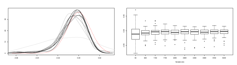
Figure 2: Sampling distribution of $S_{n}=n^{3/10}(\hat{h}_{CV,n}-h_{n0})$: kernel density estimates (left panel) and boxplots (right panel), for samples drawn from model M2 and considering values of $n$ between $50$ and $5000$. In the left panel, sharper lines correspond to larger values of $n$. The limit distribution of $S_{n}$ is also shown (dashed line).

In the next part of the study, we focused on empirically analyzing the performance of the bagged cross-validation bandwidth $\hat{h}(r,N)$, given in (15), for different values of $n$, $r$ and $N$. Figure 3 shows the sampling distribution of $\hat{h}_{n}/h_{n0}$, where $\hat{h}_{n}$ denotes either the ordinary or bagged cross-validation bandwidth. For this, 1000 samples of size $n=10^{5}$ from models M1, M2 and M3 were generated, considering in the case of $\hat{h}(r,N)$ the values $r\in\{100,500,1000,5000,10000\}$ and $N=25$. For all three models, it is observed how the bias and variance of the bagging bandwidth decrease as the subsample size increases and how its mean squared error seems to stabilize for values of $r$ close to 5000. Moreover, the behavior of the bagging selector turns out to be quite positive even when considering subsample sizes as small as $r=100$, perhaps excluding the case of model M3 for which the variance of the bagging bandwidth is still relatively high for $r=100$, although it undergoes a rapid reduction as the subsample size increases slightly.

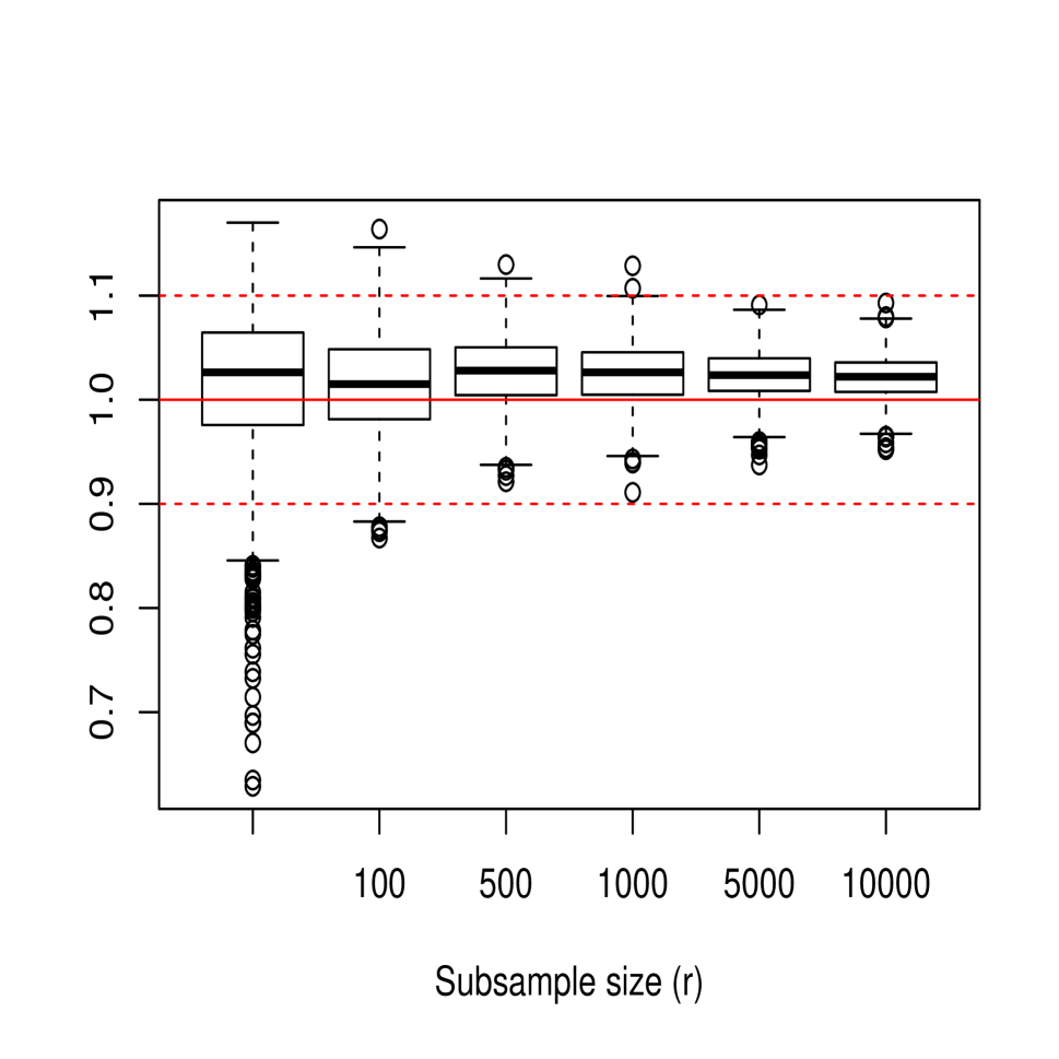
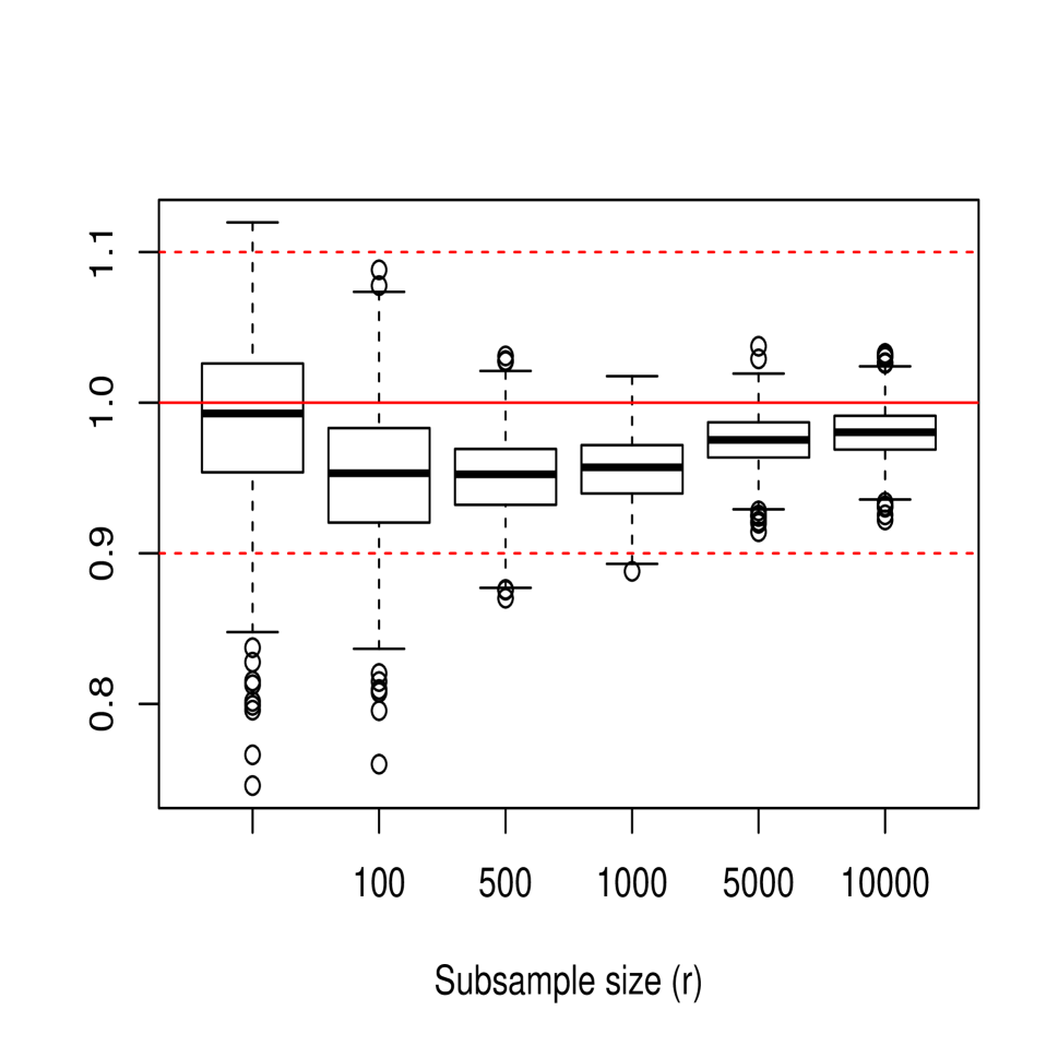
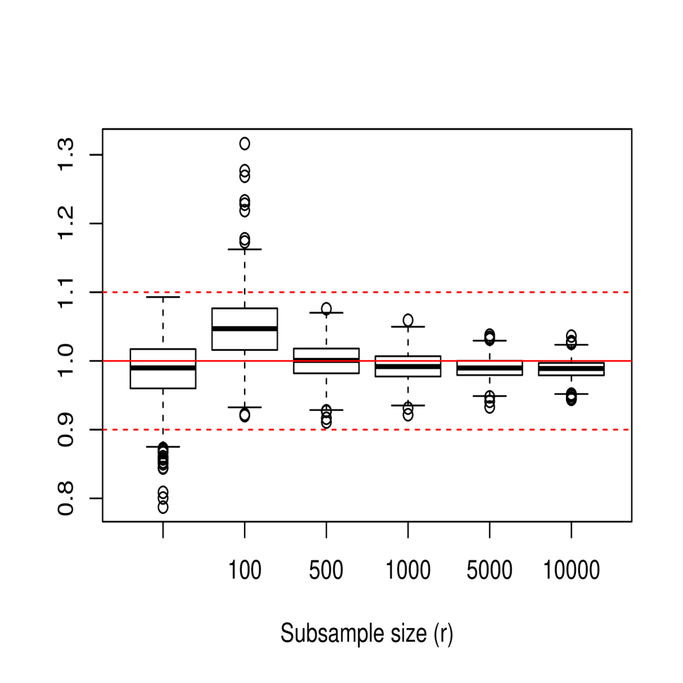
Figure 3: Sampling distribution of $\hat{h}_{CV,n}/h_{n0}$ (first boxplot on each panel) and $\hat{h}(r,N)/h_{n0}$ (second to sixth boxplots on each panel) for models M1 (left panel), M2 (central panel) and M3 (right panel), where the considered subsample sizes are $r\in\{100,500,1000,5000,10^{4}\}$ and the number of subsamples is $N=25$. The original sample size is $n=10^{5}$. Dashed lines are plotted at values 0.9 and 1.1 for reference.

The effect that $r$ has on the mean squared error of the bagged bandwidth is also illustrated in Table 1, which shows the ratio of the mean squared errors of the bagged bandwidth and the ordinary cross-validation bandwidth, MSE$[\hat{h}(r,N)]/$MSE$(\hat{h}_{CV,n})$, for the three models.

	Model
	M1	M2	M3
Subsample size ($r$)	MSE ratio
$100$	$0.47$	$1.47$	$2.16$
$500$	$0.32$	$1.06$	$0.33$
$1,000$	$0.26$	$0.80$	$0.23$
$5,000$	$0.19$	$0.30$	$0.17$
$10,000$	$0.16$	$0.22$	$0.16$

Table 1: Ratio of the mean squared errors of the bagged and the ordinary cross-validation bandwidths for models M1–M3. Different values of $r$ and $N=25$ were considered.

Apart from a better statistical precision of the cross-validation bandwidths selected using bagging, another potential advantage of employing this approach is the reduction of computing times, especially with large sample sizes. To analyze this issue, Figure 4 shows, as a function of the sample size, $n$, the CPU elapsed times for computing the standard and the bagged cross-validation bandwidths. Both variables are shown on a logarithmic scale. In the case of the bagging selector, three different subsample size values ($r$) depending on $n$ were considered: $r=n^{0.7}$, $r=n^{0.8}$ and $r=n^{0.9}$. Calculations were performed in parallel using an Intel Core i5-8600K 3.6GHz CPU. The sample size $n\in\{5000,28750,52500,76250,10^{5}\}$ and a fixed number of subsamples, $N=25$, were used. In this experiment, binning techniques were employed using a number of bins of $0.1n$ for standard cross-validation and $0.1r$ in the case of bagged cross-validation. The time required to compute the bagged cross-validation bandwidth was measured considering the three possible growth rates for $r$, mentioned above.

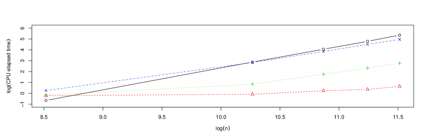
Figure 4: CPU elapsed time (seconds) as a function of the sample size of standard cross-validation (solid line-circles) and bagged cross-validation. Both variables are shown on a logarithmic scale. A fixed number of subsamples was used, $N=25$. Three growth rates for $r$ were considered, namely, $r=n^{0.7}$ (dashed line-triangles), $r=n^{0.8}$ (dotted line-pluses) and $r=n^{0.9}$ (dashed-dotted line-crosses).

Fitting an appropriate model, these CPU elapsed times could be used to predict the computing times of the different selectors for larger sample sizes. Considering Figure 4, the following log-linear model was used:

$$T(n)=\alpha n^{\beta},$$ (17)

where $T(n)$ denotes the CPU elapsed time as a function of the original sample size, $n$. In the case of the bagged cross-validation bandwidths, there is a fixed time corresponding to the one required for the setting up of the parallel socket cluster. This time, which does not depend on $n$, $r$ or $N$, but only on the CPU and the number of cores used in the parallelization, was estimated to be $0.79$. Using this value, the corrected CPU elapsed times obtained for the bagged bandwidths, $T-0.79$, were employed to fit the log-linear model (17) estimating $\alpha,\beta>0$ by least squares and, subsequently, to make predictions. Table 2 shows the predicted CPU elapsed time for ordinary and bagged cross-validation for large sample sizes. Although we should take these predictions with caution, the results in Table 2 serve to illustrate the important reductions in computing time that bagging can provide for certain choices of $r$ and $N$, especially for very large sample sizes.

	Sample size ($n$)
	$10^{6}$	$10^{7}$	$10^{8}$
Method	Computing time
Standard CV	$6$ hours	$24$ days	$7$ years
Bagged CV ($r=n^{0.7},N=25$)	$40$ seconds	$25$ minutes	$16$ hours
Bagged CV ($r=n^{0.8},N=25$)	$16$ minutes	$17$ hours	$45$ days
Bagged CV ($r=n^{0.9},N=25$)	$3$ hours	$11$ days	$2$ years

Table 2: Predicted CPU elapsed time for the standard and the bagging cross-validation method using three different choices for the subsample size.

Next, the influence of the number of subsamples, $N$, in the computing times of the bagged badwidths was studied. Similarly to Figure 4, Figure 5 shows the CPU elapsed times for computing the cross-validation bandwidths (standard and bagged). For the bagging method, the number of subsamples, $N$, was selected depending on the original sample size ($n$) by $N=\sqrt{n}$. The growth rates used for $r$ are the same as in the case of Figure 4.

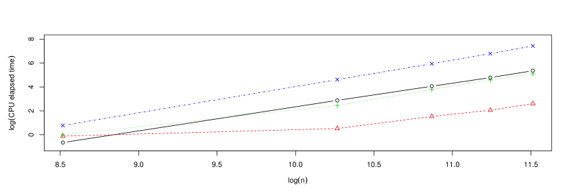
Figure 5: CPU elapsed time (seconds) as a function of the sample size of standard cross-validation (solid line-circles) and bagged cross-validation. Both variables are shown on a logarithmic scale. The number of subsamples grows with $n$ at the rate $N=\sqrt{n}$. Three growth rates for $r$ were considered, namely, $r=n^{0.7}$ (dashed line-triangles), $r=n^{0.8}$ (dotted line-pluses) and $r=n^{0.9}$ (dashed-dotted line-crosses).

It should also be stressed that although the quadratic complexity of the cross-validation algorithm is not so critical in terms of computing time for small sample sizes, even in these cases, the use of bagging can still lead to substantial reductions in mean squared error of the corresponding bandwidth selector with respect to the one selected by ordinary cross-validation. In order to show this, $1000$ samples from model M1 of sizes $n\in\{50,500,5000\}$ were simulated and the ordinary and bagged cross-validation bandwidths for each of these samples were computed. In the case of the bagged cross-validation bandwidth, both the size of the subsamples and the number of subsamples were selected depending on $n$, choosing $r=N=4\sqrt{n}$. Figure 6 shows the sampling distribution of $\hat{h}_{n}/h_{n0}$, where $\hat{h}_{n}$ denotes either the ordinary or bagged cross-validation bandwidth. In the three scenarios, it can be observed the considerable reductions in variance produced by bagging more than offset the slight increases in bias, thus obtaining significant reductions in mean squared error with respect to the ordinary cross-validation bandwidth selector. Specifically, the relative reductions in mean squared error achieved by the bagged bandwidth turned out to be $69.3\%$, $90.1\%$ and $93.8\%$ for $n=50$, $n=500$ and $n=5000$, respectively. This experiment was repeated with models M2 and M3, obtaining similar results.

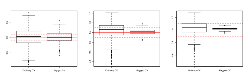
Figure 6: Sampling distribution of $\hat{h}_{n}/h_{n0}$, where $\hat{h}_{n}$ denotes either the ordinary or bagged cross-validation bandwidth, for samples of size $n=50$ (left panel), $n=500$ (central panel) and $n=5,000$ (right panel) drawn from model M1. The values of $r$ and $N$ were chosen as $r=N=4\sqrt{n}$. Dashed lines are plotted at values 0.9 and 1.1 for reference.

7 Application to COVID-19 data

In order to illustrate the performance of the techniques studied in the previous sections, the COVID-19 dataset briefly mentioned in the introduction is considered. It consists of a sample of size $n=105,235$ which contains the age (the explanatory variable) and the time in hospital (the response variable) of people infected with COVID-19 in Spain from January 1, 2020 to December 20, 2020. Due to the high number of ties in this dataset and in order to avoid problems when performing cross-validation, we decided to remove the ties by jittering the data. In particular, three independent random samples of size $n$, $U_{1}$, $U_{2}$ and $U_{3}$, drawn from a continuous uniform distribution defined on the interval $(0,1)$, were generated. Then, $U_{1}$ was added to the original explanatory variable and $U_{2}-U_{3}$ to the original response variable. Figure 7 shows scatterplots for the complete sample as well as for three randomly chosen subsamples of size $1,000$.

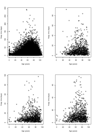
Figure 7: Whole COVID-19 sample (top left panel) as well as three randomly chosen subsamples of size $1000$.

To compute the standard cross-validation bandwidth using binning, the number of bins was set to $10,000$, that is, roughly $10\%$ of the sample size. The value of the bandwidth thus obtained was $1.84$ and computing it took $72$ seconds. For the bagged bandwidth, $10$ subsamples of size $30,000$ were considered. Binning was used again for each subsample, fixing the number of bins to $3,000$. The calculations associated with each subsample were performed in parallel using $5$ cores. The value of the bagged bandwidth was $1.52$ and its computing time was $33$ seconds. Figure 8 shows the Nadaraya–Watson estimates with both standard and bagged cross-validation bandwidths. For comparative purposes, the local linear regression estimate with direct plug-in bandwidth (Ruppert et al.,, 1995) was also computed.

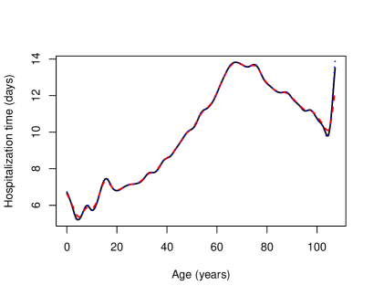
Figure 8: Kernel regression estimates for the COVID-19 data. The Nadaraya–Watson estimator with standard (dashed line) and bagged (solid line) cross-validation bandwidths are shown. Additionally, the local linear estimator with plug-in bandwidth (dotted line) is also presented.

Figure 8 shows that the Nadaraya–Watson estimator with standard cross-validation bandwidth produces a slightly smoother estimate than the one obtained with the bagged bandwidth, the latter being almost indistinguishable from the local linear estimate computed with direct plug-in bandwidth. One can conclude that the expected time that a person infected with COVID-19 will remain in hospital increases non-linearly with age for people under approximately $70$ years. This trend is reversed for people aged between $70$ and $100$ years. This could be due to the fact that patients in this age group are more likely to die and, therefore, end the hospitalization period prematurely. Finally, the expected hospitalization time grows again very rapidly with age for people over $100$ years of age, although this could be caused by some boundary effect, since the number of observations for people over $100$ years old is very small, specifically $155$, which corresponds to roughly $0.15\%$ of the total number of observations. In order to avoid this possible boundary effect, the estimators were also fitted to a modified version of the sample in which the explanatory variable was transformed using its own empirical distribution function. The resulting estimators are shown in Figure 9, where the explanatory variable was returned to its original scale by means of its empirical quantile function.

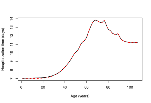
Figure 9: Kernel regression estimators for the COVID-19 data, removing boundary effects. The Nadaraya–Watson estimator with standard (dashed line) and bagged (solid line) cross-validation bandwidths are shown.

Finally, the same procedure was followed to estimate the expected time in hospital but splitting the patients by gender, as shown in Figure 10. This figure shows that the expected time in hospital is generally shorter for women, except for ages less than $30$ years or between $65$ and $85$ years. Anyhow, the difference in mean time in hospital for men and women never seems to exceed one day. In Figure 10, only the Nadaraya–Watson estimates computed with the bagged cross-validation bandwidths ($h=0.03$ for men and $h=0.028$ for women) are shown. Both the Nadaraya–Watson estimates with standard cross-validation bandwidths ($h=0.028$ for men and $h=0.023$ for women) and the local linear estimates with direct plug-in bandwidths produced very similar and graphically indistinguishable results from those shown in Figure 10.

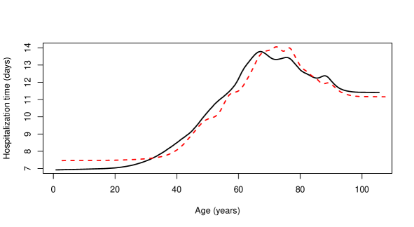
Figure 10: Kernel regression estimators for the COVID-19 data by gender, removing boundary effects. The Nadaraya–Watson estimators with bagged cross-validation bandwidths are shown for male (solid line) and female (dashed line) patients.

8 Discussion

The asymptotic properties of the leave-one-out cross-validation bandwidth for the Nadaraya–Watson estimator considering a regression model with random design have been studied in this paper. Additionally, a bagged cross-validation selector have been also analyzed (theoretically and empirically) as an alternative to standard leave-one-out cross-validation. The advantage of this bandwidth selector is twofold: (i) to gain computational efficiency with respect to standard leave-one-out cross-validation by applying the cross-validation algorithm to several subsamples of size $r<n$ rather than a single sample of size $n$, and (ii) to reduce the variability of the leave-one-out cross-validation bandwidth. Although the new bandwidth selector studied in the present paper can outperform the behavior of the standard cross-validation selector even for moderate sample sizes, improvements in computation time become truly significant only for large-sized samples.

The methodology presented in this paper can be applied to other bandwidth selection techniques, apart from cross-validation, as mentioned in Barreiro-Ures et al., (2020). Extensions to bootstrap bandwidth selectors is an interesting topic for a future research. The bootstrap resampling plans proposed by Cao and González-Manteiga, (1993) can be used to derive a closed form for the bootstrap criterion function in nonparametric regression estimation, along the lines presented by Barbeito et al., (2021) who have dealt with matching and prediction.

Another interesting future research topic is the extension of the results presented in this paper to the case of the local linear estimator, whose behavior is known to be superior to that of the Nadaraya–Watson estimator, especially in the boundary regions.

Supplementary Materials

Supplementary materials include proofs and some plots completing the simulation study.

Funding

This research has been supported by MINECO grant MTM2017-82724-R, and by Xunta de Galicia (Grupos de Referencia Competitiva ED431C-2020-14 and Centro de Investigación del Sistema Universitario de Galicia ED431G 2019/01), all of them through the ERDF.

References

- Barbeito, (2020) Barbeito, I. (2020). Exact bootstrap methods for nonparametric curve estimation. PhD thesis, Universidade da Coruña. https://ruc.udc.es/dspace/handle/2183/26466.
- Barbeito et al., (2021) Barbeito, I., Cao, R., and Sperlich, S. (2021). Bandwidth selection for statistical matching and prediction. Technical report, University of A Coruña. Department of Mathematics. http://dm.udc.es/preprint/Bandwidth_Selection_Matching_Prediction_NOT_BLINDED.pdf and http://dm.udc.es/preprint/SuppMaterial_Bandwidth_Selection_Matching_Prediction_NOT_BLINDED.pdf.
- Barreiro-Ures et al., (2020) Barreiro-Ures, D., Cao, R., Francisco-Fernández, M., and Hart, J. D. (2020). Bagging cross-validated bandwidths with application to big data. Biometrika. https://doi.org/10.1093/biomet/asaa092.
- Breiman, (1996) Breiman, L. (1996). Bagging predictors. Machine Learning, 24:123–140.
- Cao and González-Manteiga, (1993) Cao, R. and González-Manteiga, W. (1993). Bootstrap methods in regression smoothing. Journal of Nonparametric Statistics, 2(4):379–388.
- Cleveland, (1979) Cleveland, W. S. (1979). Robust locally weighted regression and smoothing scatterplots. Journal of the American Statistical Association, 74(368):829–836.
- Fan, (1992) Fan, J. (1992). Design-adaptive nonparametric regression. Journal of the American Statistical Association, 87(420):998–1004.
- Friedman and Hall, (2007) Friedman, J. H. and Hall, P. (2007). On bagging and nonlinear estimation. Journal of Statistical Planning and Inference, 137:669–683.
- Hall and Robinson, (2009) Hall, P. and Robinson, A. P. (2009). Reducing variability of crossvalidation for smoothing parameter choice. Biometrika, 96(1):175–186.
- Härdle et al., (1988) Härdle, W., Hall, P., and Marron, J. S. (1988). How far are automatically chosen regression smoothing parameters from their optimum? Journal of the American Statistical Association, 83(401):86–95.
- Köhler et al., (2014) Köhler, M., Schindler, A., and Sperlich, S. (2014). A review and comparison of bandwidth selection methods for kernel regression. International Statistical Review / Revue Internationale de Statistique, 82(2):243–274.
- Nadaraya, (1964) Nadaraya, E. A. (1964). On estimating regression. Theory of Probability & Its Applications, 9(1):141–142.
- Opitz and Maclin, (1999) Opitz, D. and Maclin, R. (1999). Popular ensemble methods: an empirical study. Journal of Artificial Intelligence Research, 11:169–198.
- Ruppert et al., (1995) Ruppert, D., Sheather, S. J., and Wand, M. P. (1995). An effective bandwidth selector for local least squares regression. Journal of the American Statistical Association, 90(432):1257–1270.
- Stone, (1977) Stone, C. J. (1977). Consistent nonparametric regression. The Annals of Statistics, 5(4):595–620.
- Stone, (1974) Stone, M. (1974). Cross-validatory choice and assessment of statistical predictions. Journal of the Royal Statistical Society, Series B, 36:111–147.
- Wand and Jones, (1995) Wand, M. P. and Jones, M. C. (1995). Kernel smoothing. Chapman and Hall, London.
- Watson, (1964) Watson, G. S. (1964). Smooth regression analysis. Sankhyā: The Indian Journal of Statistics, Series A, 26(4):359–372.