Parameter-free Gradient Temporal Difference Learning

Abstract

Reinforcement learning lies at the intersection of several challenges. Many applications of interest involve extremely large state spaces, requiring function approximation to enable tractable computation. In addition, the learner has only a single stream of experience with which to evaluate a large number of possible courses of action, necessitating algorithms which can learn off-policy. However, the combination of off-policy learning with function approximation leads to divergence of temporal difference methods. Recent work into gradient-based temporal difference methods has promised a path to stability, but at the cost of expensive hyperparameter tuning. In parallel, progress in online learning has provided parameter-free methods that achieve minimax optimal guarantees up to logarithmic terms, but their application in reinforcement learning has yet to be explored. In this work, we combine these two lines of attack, deriving parameter-free, gradient-based temporal difference algorithms. Our algorithms run in linear time and achieve high-probability convergence guarantees matching those of GTD2 up to $\log$ factors. Our experiments demonstrate that our methods maintain high prediction performance relative to fully-tuned baselines, with no tuning whatsoever.

1 Introduction

A central problem in reinforcement learning (RL) is policy evaluation: given a course of action — otherwise known as a policy — what is its expected long-term outcome? Policy evaluation is an essential step in policy iteration schemes, facilitates model-based planning (Grimm et al., 2020), and in recent years has even found applications in representation learning (Veeriah et al., 2019; Schlegel et al., 2021).

Temporal difference (TD) methods (Sutton, 1988) comprise the most popular class of policy-evaluation algorithms, leveraging approximate dynamic programming approaches to perform credit assignment incrementally. Nevertheless, a notable deficiency is that they require a step-size, which determines the pace of adapting value function estimates to the current data point. A step-size that is too high may impede convergence and stability, while a step-size that is too low can stall progress. Some TD algorithms that enjoy other desirable properties, such as Gradient-TD (GTD) methods (Liu et al., 2018) that can be shown to converge where other TD methods do not (Baird, 1995), but can be incredibly sensitive to the step-size. Generally, selection of the step-size and other parameters — known as tuning — requires massive amounts of computation time, to the extent that this tuning has become an impediment to reliable scientific results (Henderson et al., 2018, 2019).

Various approaches have been proposed to alleviate these difficulties. Step-size schedules leading to optimal convergence rates and robust guarantees are well-known in the stochastic optimization literature (Nemirovski et al., 2009; Ghadimi & Lan, 2013), but they often depend on problem-dependent quantities that are unavailable to the practitioner. Meta-descent methods such as Stochatic Meta-descent (Schraudolph, 1999) and TIDBD (Kearney et al., 2018) instead learn a step-size according to some meta-objective, thereby obviating the need to tune one. Yet these methods inevitably introduce new parameters to be tuned, such as a meta-stepsize, decay parameter parameter, etc, and can be quite sensitive to these new parameters in practice (Jacobsen et al., 2019). Quasi second-order methods adopted from the deep learning community — such as the well-known Adam algorithm (Kingma & Ba, 2014) — can be effective in practice but have no theoretical guarantees when applied to TD methods. Further, while these quasi second-order methods are often less sensitive to their parameters, they never fully manage to remove the need for parameter tuning completely.

To address these deficiencies, we adapt recent work on parameter-free online learning to policy evaluation. We leverage a series of black-box reductions to reduce policy evaluation to a problem that can be solved using a powerful class of online linear optimization (OLO) algorithm based on betting strategies (Orabona & Pál, 2016; Orabona, 2019; Cutkosky & Orabona, 2018). The key characteristic of these approaches is that they require no parameter tuning, yet guarantee near-optimal regret bounds. We construct our algorithms in such a way that they avoid requiring any a priori information about problem-dependent constants, while still making high-probability guarantees and achieving similar performance to fully-tuned baselines.

2 Preliminaries

Reinforcement learning (RL) is a framework in which a decision-maker (the agent) learns via repeated trial-and-error interaction with its environment. The environment is formalized as a Markov decision process $(\mathcal{S},\mathcal{A},P,R)$, where $\mathcal{S}$ and $\mathcal{A}$ are sets of states and actions, $P(s^{\prime}|s,a)$ is a transition kernel specifying the probability of transitioning to state $s^{\prime}\in\mathcal{S}$ when taking action $a\in\mathcal{A}$ in state $s\in\mathcal{S}$, and $R:\mathcal{S}\times\mathcal{A}\rightarrow\mathbb{R}$ is a reward function mapping state-action pairs to rewards. At each discrete time-step $t\in\mathbb{N}$, the agent observes the current state $S_{t}\in\mathcal{S}$ and selects an action $A_{t}$ according to policy $\pi:\mathcal{S}\times\mathcal{A}\rightarrow[0,1]$. The value function $v^{\pi}$ is the expected discounted reward when following policy $\pi$ from state $s$:

$$v^{\pi}(s)=\mathbb{E}\left[\sum_{k=0}^{\infty}\gamma^{k}R_{t+k}|S_{0}=s\right],$$

where $\gamma\in[0,1)$ is a constant discount factor and $R_{t}$ denotes $R(S_{t},A_{t})$. The process of estimating $v^{\pi}$ is referred to as policy evaluation.

When $|\mathcal{S}|$ is large, it is common to estimate $v^{\pi}$ using parametric function approximation. A simple yet often effective strategy is to approximate $v^{\pi}$ with a linear approximation. We assume access to a feature map $\phi:\mathcal{S}\rightarrow\mathbb{R}^{d}$ which maps each state to a vector of features, and approximate $\hat{v}^{\pi}(s)=\theta^{\top}\phi(s)\approx v^{\pi}(s)$. In vector form, we write $V^{\pi}\in\mathbb{R}^{|S|}$ and $\hat{V}^{\pi}=\Phi\theta$, where $\Phi\in\mathbb{R}^{|\mathcal{S}|\times d}$ is the matrix with rows $\phi(s)$.

In practice, the learner may have several candidate policies to choose between. Rather than evaluating each of them separately, it is often desirable to evaluate them simultaneously, in parallel, while following some sufficiently exploratory behavior policy $\pi_{b}$. This is off-policy evaluation. In particular, given a target policy $\pi$, we would like to estimate estimate $V^{\pi}$ using a dataset of $T\in\mathbb{N}$ transitions $\mathcal{D}\overset{\text{def}}{=}\left\{(s_{t},a_{t},r_{t},s_{t}^{\prime})\right\}_{t=1}^{T}$, where $s_{t}\sim\xi(\cdot)$ for some state distribution $\xi$, $a_{t}\sim\pi_{b}(\cdot|s_{t})$, $r_{t}=R(s_{t},a_{t})$, and $s_{t}^{\prime}\sim P(\cdot|s_{t},a_{t})$. For a given transition $(s_{t},a_{t},r_{t},s_{t}^{\prime})\in\mathcal{D}$ we denote the importance sampling ratio $\rho_{t}\overset{\text{def}}{=}\frac{\pi(a_{t}|s_{t})}{\pi_{b}(a_{t}|s_{t})}$, the shorthands $\phi_{t}\overset{\text{def}}{=}\phi(s_{t})$ and $\phi_{t}^{\prime}\overset{\text{def}}{=}\phi(s_{t}^{\prime})$, the TD error $\delta_{t}\overset{\text{def}}{=}r_{t}+\gamma\theta^{\top}\phi_{t}^{\prime}-\theta^{\top}\phi_{t}$, and $\Xi\overset{\text{def}}{=}\text{diag}(\xi)\in\mathbb{R}^{|\mathcal{S}|\times|\mathcal{S}|}$ the diagonal matrix induced by the state distribution. Finally, in what follows we will make use of the following definitions

$$\hat{A}_{t}\overset{\text{def}}{=}\rho_{t}\phi_{t}(\phi_{t}-\gamma\phi_{t}^{\prime})^{\top},\ \ \hat{b}_{t}\overset{\text{def}}{=}\rho_{t}r_{t}\phi_{t},\ \ \hat{C}_{t}\overset{\text{def}}{=}\phi_{t}\phi_{t}^{\top}$$ (1)

and their expectations $A\overset{\text{def}}{=}\mathbb{E}[\hat{A}_{t}]$, $b\overset{\text{def}}{=}\mathbb{E}[\hat{b}_{t}]$ $C\overset{\text{def}}{=}\mathbb{E}[\hat{C}_{t}]$.

Gradient-based Temporal Difference Learning. Under both function approximation and off-policy sampling, classic TD algorithms can fail to converge for any scalar step-sizes (Baird, 1995). Specifically, in the off-policy setting, $\xi$ is generally neither the stationary distribution of $\pi$ nor the discounted future state visitation distribution. In this case, $A$ can fail to be positive-definite, which could lead to non-convergence of the resulting dynamical system.

This deficiency has motivated attempts to reformulate the typical TD algorithms as stochastic gradient methods. These gradient-based TD (GTD) methods seek to minimize the Norm of the Expected Update (NEU), or the Mean-square Projected Bellman Error (MSPBE), either of which can be described by the objective function

$$J(\theta)=\|\Phi^{\top}\Xi(\mathcal{B}^{\pi}\hat{V}^{\pi}-\hat{V}^{\pi})\|^{2}_{M^{{-1}}}=\|b-A\theta\|_{M^{{-1}}},$$ (2)

where $\mathcal{B}^{\pi}$ is the Bellman operator (Liu et al., 2018). The NEU is captured by setting $M=I$, and the MSPBE via $M=\mathbb{E}[\phi_{t}\phi_{t}^{\top}]$.

In this paper, we leverage the saddle-point (SP) formulation in Liu et al. (2018). Minimization of $J(\theta)$ can be equivalently formulated as the following SP problem:

$$\min_{\theta\in\Theta}\max_{y\in\mathcal{Y}}\left\{L(\theta,y)\overset{\text{def}}{=}\langle b-A\theta,y\rangle-\frac{1}{2}\|y\|^{2}_{M}\right\},$$ (3)

where $\Theta\subset\mathbb{R}^{d}$ and $\mathcal{Y}\subset\mathbb{R}^{d}$ are assumed convex and compact. The quality of a candidate solution $(\theta,y)\in\Theta\times\mathcal{Y}$ is measured in terms of the duality gap:

$$\max_{y^{*}\in\mathcal{Y}}L(\theta,y^{*})-\min_{\theta^{*}\in\Theta}L(\theta^{*},y).$$ (4)

It can be shown that this quantity is non-negative, and any point $(\theta,y)$ for which $\max_{y^{*}\in\mathcal{Y}}L(\theta,y^{*})-\min_{\theta^{*}\in\Theta}L(\theta^{*},y)=0$ is a saddle-point of the SP problem 3 (see Appendix A). Further, it is known that if $(\theta^{*},y^{*})$ is a saddle-point of Equation 3, then $\theta^{*}$ is a minimizer of the MSPBE (Liu et al., 2018).

Notations. In what follows, we assume for simplicity that $\Theta$ and $\mathcal{Y}$ are equipped with norms $\|\cdot\|=\|\cdot\|_{2}$. For a PSD matrix $M$ we denote $\|x\|_{M}^{2}\overset{\text{def}}{=}\langle x,Mx\rangle$. The decision sets $\Theta$ and $\mathcal{Y}$ are assumed compact and convex, and we denote $D\overset{\text{def}}{=}\max\left\{\max_{\theta\in\Theta}\|\theta\|,\max_{y\in\mathcal{Y}}\|y\|\right\}$ and $D_{\infty}\overset{\text{def}}{=}\max\left\{\max_{\theta\in\Theta}\|\theta\|_{\infty},\max_{y\in\mathcal{Y}}\|y\|_{\infty}\right\}$. Given a closed convex set $W$, we define the projection $\Pi_{W}(w)=\operatorname{arg\,min}_{\hat{w}\in W}\|\hat{w}-w\|$. The notation $O(\cdot)$ hides constant terms and $\widetilde{O}(\cdot)$ additionally hides log terms. Throughout this work, we will denote $g_{t}^{\theta}=\mathbb{E}[\hat{g}_{t}^{\theta}|\theta_{t},y_{t}]\in\partial_{\theta}L(\theta_{t},y_{t})$ and $g_{t}^{y}=\mathbb{E}[\hat{g}_{t}^{y}|\theta_{t},y_{t}]\in-\partial_{y}L(\theta_{t},y_{t})$, with $\hat{g}_{t}^{\theta}$ and $\hat{g}_{t}^{y}$ denoting stochastic subgradients of Equation 3. Concretely,

$${\hat{g}}_{t}^{\theta}=-\hat{A}_{t}^{\top}y_{t},\qquad{\hat{g}}_{t}^{y}=-\hat{b}_{t}+\hat{A}_{t}\theta_{t}+\hat{M}_{t}y_{t}.$$ (5)

It will often be convenient to work directly with the joint space $\Theta\times\mathcal{Y}$, which we endow with norms $\|(\theta,y)\|\overset{\text{def}}{=}\sqrt{\|\theta\|^{2}+\|y\|^{2}}$ and $\|(\theta,y)\|_{\infty}=\max\left\{\|\theta\|_{\infty},\|y\|_{\infty}\right\}$. When clear from context, we will denote $g_{t}\overset{\text{def}}{=}(g_{t}^{\theta},g_{t}^{y})$, ${\hat{g}}_{t}\overset{\text{def}}{=}({\hat{g}}_{t}^{\theta},{\hat{g}}_{t}^{y})$, $z_{t}\overset{\text{def}}{=}(\theta_{t},y_{t})$ and $z^{*}\overset{\text{def}}{=}(\theta^{*},y^{*})$.

Assumptions. Throughout this work we make the following standard assumptions

1. (feasibile sets) The feasible sets $\Theta$ and $\mathcal{Y}$ are assumed to be compact and convex, and the the solution $(\theta^{*},y^{*})$ of SP problem 3 is assumed to belong to $\Theta\times\mathcal{Y}$.

2. (non-singularity) The covariance matrix $C=\mathbb{E}\left[\phi_{t}\phi_{t}^{\top}\right]=\Phi^{\top}D\Phi$ and $A=\mathbb{E}\left[\rho_{t}\phi_{t}(\phi_{t}-\gamma\phi_{t}^{\prime})^{\top}\right]$ are assumed to be non-singular.

3. (boundedness) The features $(\phi_{t},\phi_{t}^{\prime})$ have uniformly bounded second moments. Furthermore, we assume the upperbounds $\max_{t}\|\phi_{t}\|_{\infty}\leq L$, $\rho_{t}\leq\rho_{\max}$, and $R(s_{t},a_{t})\leq R_{\max}$ exist and are finite for all $t\in[T]$.

Together assumptions A2 and A3 imply the existence of values $G_{\theta},G_{y},\sigma_{\theta},\sigma_{y}\in\mathbb{R}$ and such that for $g_{t},{\hat{g}}_{t}\in\Theta\times\mathcal{Y}$ with $\mathbb{E}\left[{\hat{g}}_{t}|\theta_{t},y_{t}\right]=g_{t}$, the following bounds hold

$$\mathbb{E}\left[\|{\hat{g}}_{t}\|^{2}\right] \leq G^{2}\overset{\text{def}}{=}G_{\theta}^{2}+G_{y}^{2}$$ (6)

$$\mathbb{E}\left[\|{\hat{g}}_{t}-g_{t}\|^{2}\right] \leq\sigma^{2}\overset{\text{def}}{=}\sigma_{\theta}^{2}+\sigma_{y}^{2}$$ (7)

3 Parameter-free Gradient Temporal Difference Learning

In this section, we derive parameter-free algorithms for off-policy policy evaluation with linear function approximation. Our approach proceeds in three steps. In Section 3.1, we first reduce our policy evaluation problem to an online learning problem, and show that the performance guarantees of the GTD2 algorithm can be matched using any online learning algorithm exhibiting a particular kind of adaptivity — this will enable us to make robust guarantees without appealing to any hyperparameters of the algorithm in question. Section 3.2 then discusses a class of online learning algorithm which avoids tuning step-sizes while maintaining near-optimal guarantees, as well as an algorithmic component that will make their use more practical in our problem setting. Finally, in Section 3.3 we present our proposed algorithm, PFGTD+.

3.1 From Saddle-point Optimization to OLO

Our first step is to reduce our saddle-point problem (Equation 3) to an OLO problem. Luckily, the structure of Equation 3 makes this easy: at each time $t$ we can simply compute the stochastic subgradients (as given in Equation 5) and pass them along to an OLO algorithm $\mathcal{A}$, as shown in Algorithm 1. As the following theorem then shows, we need not make any assumptions about the internals of $\mathcal{A}$ to obtain a high-probability bound on the duality gap — we only require that $\mathcal{A}$ exhibits a particular form of adaptivity to the sequence of subgradients.

  Input: Online Learning algorithm $\mathcal{A}$, dataset $\mathcal{D}=\left\{\phi_{t},a_{t},r_{t},\phi_{t}^{\prime},\rho_{t}\right\}_{t=1}^{T}$, policies $\pi$ and $\pi_{b}$

  for $t=1:T$ do

     Get $\theta_{t}$ and $y_{t}$ from $\mathcal{A}$

     Set $\hat{A}_{t}=\rho_{t}\phi_{t}\left(\phi_{t}-\gamma\phi_{t}^{\prime}\right)^{\top}$, $\hat{b}_{t}=\rho_{t}r_{t}\phi_{t}$, $\hat{M}_{t}=\phi_{t}\phi_{t}^{\top}$

     Set $\hat{g}_{t}^{\theta}=-\hat{A}_{t}^{\top}y_{t}$ and $\hat{g}_{t}^{y}=\hat{A}_{t}\theta_{t}-\hat{b}_{t}+\hat{M}_{t}y_{t}$

     Send $\hat{g}_{t}^{\theta}$ and $\hat{g}_{t}^{y}$ to $\mathcal{A}$ as the $t^{\text{th}}$ subgradients

  end for

  Return: average iterates $\overline{\theta}_{T}=\frac{1}{T}\sum_{t=1}^{T}\theta_{t}$, $\overline{y}_{T}=\frac{1}{T}\sum_{t=1}^{T}y_{t}$

Algorithm 1 Saddle-point to Online Learning Reduction

Theorem 1

Suppose that for any $u\in\Theta\times\mathcal{Y}$, online learning algorithm $\mathcal{A}$ guarantees regret

$$R_{T}^{\mathcal{A}}(u)=\sum_{t=1}^{T}\langle g_{t},z_{t}-u\rangle\leq A_{T}(u)+B_{T}(u)\sqrt{\sum_{t=1}^{T}\|g_{t}\|^{2}}$$

where $A_{T}$ and $B_{T}$ are arbitrary deterministic, non-negative functions. Then under Assumptions A1-A3, Algorithm 1 guarantees

$$\mathbb{E}\left[\max_{y^{*}\in\mathcal{Y}}L(\overline{\theta}_{T},y^{*})-\min_{\theta^{*}\in\Theta}L(\theta^{*},\overline{y}_{T})\right]$$

$$\qquad\leq\frac{A_{T}(z^{*})}{T}+\frac{B_{T}(z^{*})D\Big{(}2\|A\|+\lambda+\frac{\sigma+\|b\|}{D}\Big{)}}{\sqrt{T}},$$

where $\lambda=\lambda_{\max{}}(M)$. Further, if the light-tailed condition $\mathbb{E}\left[\exp\left(\frac{\|{\hat{g}}_{t}\|^{2}}{G^{2}}\right)\right]\leq\exp\left(1\right)$ holds, then for any $\delta>0$, Algorithm 1 guarantees with probability at least $1-\delta$

$$\max_{y^{*}\in\mathcal{Y}}L(\overline{\theta}_{T},y^{*})-\min_{\theta^{*}\in\Theta}L(\theta^{*},\overline{y}_{T})\leq$$

$$\frac{A_{T}(z^{*})}{T}+\frac{\Big{(}1+\log\left(\frac{2}{\delta}\right)\Big{)}B_{T}^{\delta}(z^{*})D\Big{(}2\|A\|+\lambda+\frac{\sigma+\|b\|}{D}\Big{)}}{\sqrt{T}},$$

where $B_{T}^{\delta}(z^{*})=2\max\Big{\{}B_{T}(z^{*}),\linebreak[1]\frac{4D}{\sqrt{1+\log\left(2/\delta\right)}}\Big{\}}$.

Proof of this theorem can be found in Appendix B. Theorem 1 tells us that the sample complexity $O\Big{(}\frac{\|A\|+\lambda_{\max}(M)+\sigma}{\sqrt{T}}\Big{)}$ of GTD2 can be matched up to the coefficients $A_{T}$ and $B_{T}$ by any algorithm which achieves the so-called second-order regret bound $R_{T}\leq O\Big{(}\sqrt{\sum_{t=1}^{T}\|g_{t}\|^{2}}\Big{)}$, and that these guarantees will hold with high probability. Notably, the result makes no appeal to step-sizes. In fact, the theorem assumes nothing at all about the internals of $\mathcal{A}$, constrasting the high-probability bounds derived in Liu et al. (2018) which require a particular choice of step-size. This would be problematic for our purposes, as our algorithms will not have a step-size to tune in the first place! Finally, we note that attaining high-probability bounds with parameter-free algorithms is generally an open problem (Jun & Orabona, 2019), and Theorem 1 is the first that we are aware of. Generalizing this result to a broader class of stochastic optimization problems is an exciting direction for future work.

3.2 Algorithms for Parameter-free Learning

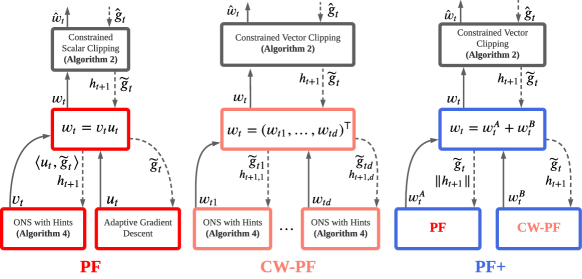
Figure 1: Diagrams of the three different parameter-free OLO procedures studied in this paper (best viewed in color). Each procedure consists of Algorithm 2, followed by one of three sub-procedures: PF, CW-PF, or PF+. Decisions made by each reduction in the hierarchy are propagated from bottom to top along the solid arrows, and feedback is propagated from the top down along the dashed arrows. Adaptive Gradient Descent in the PF routine refers to gradient descent over domain $\left\{x\in\mathbb{R}^{d}:\|x\|\leq 1\right\}$ with step-sizes $\eta_{t}=\sqrt{2}/2\sqrt{\sum_{\tau=1}^{t}\|\widetilde{g}_{\tau}\|^{2}}$. Pseudocode is additionally provided in Appendix D.

Given the reduction of the previous section, our policy evaluation problem can be solved by any OLO algorithm which achieves an adaptive regret bound of the form $R_{T}(u)\leq O\Big{(}\sqrt{\sum_{t=1}^{T}\|g_{t}\|^{2}}\Big{)}$. We additionally want to achieve such a bound without any hyperparameter tuning. Interestingly, we can achieve both of these goals by instead setting our sights on a stronger bound of the form $R_{T}(u)\leq O\Big{(}\|u\|\sqrt{\sum_{t=1}^{T}\|g_{t}\|^{2}}\Big{)}$ — the parameter-free regret bound. Bounds of this form are what would be achieved if online (sub)gradient descent could be applied with the fixed stepsize $\eta^{*}=\|u\|/\sqrt{\sum_{t=1}^{T}\|g_{t}\|^{2}}$, yielding the optimal dependence on both the comparator $u$ and the sequence of subgradients $(g_{t})_{t=1}^{T}$ (see Orabona (2019, Theorem 2.13)). Unfortunately, this step-size cannot be chosen as it involves quantities unknown to the learner in advance, and in fact it turns out that these bounds can not be obtained without prior knowledge of $u$ (Orabona & Pál, 2018). However, several recent works make guarantees of this form up to $\log$ factors, particularly those operating in the coin-betting framework (Cutkosky & Orabona, 2018; Orabona & Pál, 2016).

In the coin-betting framework, the objective of guaranteeing low regret $R_{T}=\sum_{t=1}^{T}\langle g_{t},w_{t}-u\rangle$ is re-cast as a betting problem in which the objective is to guarantee high wealth, $W_{T}\overset{\text{def}}{=}W_{0}-\sum_{t=1}^{T}\langle g_{t},w_{t}\rangle$, starting from some initial endowment of $W_{0}$. Concretely, in the 1-dimensional OLO case, at each time $t\in[T]$ the learner places a bet $w_{t}=\beta_{t}W_{t-1}$ — corresponding to some (signed) fraction $\beta_{t}\in[-1,1]$ of their current wealth $W_{t-1}$ — on the outcome of a continuous-valued “coin” $-g_{t}$. The learner wins (or loses) the amount $-g_{t}w_{t}$, and their wealth becomes $W_{t}=W_{t-1}-g_{t}w_{t}=W_{t-1}(1-\beta_{t}g_{t})$. The key observation making this a viable strategy is that any algorithm which guarantees $W_{T}\geq F(\sum_{t}-g_{t})$ for some convex $F$ also guarantees $R_{T}(u)\leq F^{*}(u)+W_{0}$, where $F^{*}$ denotes the Fenchel dual of $F$ (McMahan & Orabona, 2014).

To use these approaches in our problem setting, we must address some subtle issues. First, on each round coin-betting algorithms make bets of the form $w_{t}=\beta_{t}W_{t}$ and seek to maximize the wealth $W_{T}$ — this makes coin-betting algorithms more naturally suited to unbounded domains, in which $\|w_{t}\|$ can be arbitrarily large. This is not always an appropriate assumption for our problems, in which numerical stability may be a concern in deployment. Second, recall that in response to choosing betting fraction $\beta_{t}$, the wealth becomes $W_{t+1}=W_{t}(1-g_{t}\beta_{t})$ — this procedure only makes sense if the wealth is always non-negative, requiring that $|\beta_{t}|\leq 1/|g_{t}|$. Yet $\beta_{t}$ is chosen before observing $g_{t}$, so ensuring non-negative wealth requires knowing a bound $G\geq|g_{t}|$ in advance. In practice, this is somewhat unsatisfying because such a bound is either completely unknown a priori or is difficult to compute.

  Input: Algorithm $\mathcal{A}$ that takes hints, initial value $\mathfrak{g}$, scaling function $\mathcal{M}$

  Initialize: initial hint $h_{1}=\mathfrak{g}$

  for $t=1:T$ do

     Get $w_{t}$ from $\mathcal{A}$

     Play $\hat{w}_{t}=\Pi_{\mathcal{W}}(w_{t})$, Receive $\hat{g}_{t}\in\partial\ell_{t}(\hat{w}_{t})$

     

     // Gradient Clipping (Algorithm 3)

     Set $g^{\text{trunc}}_{t}=\begin{cases}h_{t}\dfrac{\hat{g}_{t}}{\mathcal{M}(\hat{g}_{t})}\qquad&\text{ if }\mathcal{M}(\hat{g}_{t})>h_{t}\\ \hat{g}_{t}&\text{ otherwise}\end{cases}$

     Update $h_{t+1}=\max\Big{(}h_{t},\mathcal{M}(\hat{g}_{t})\Big{)}$

     

     // Constraint-set reduction (Algorithm 6)

     Set $S(w)=\|w-\Pi_{\mathcal{W}}(w)\|$,  $\widetilde{w}_{t}=\frac{w_{t}-\hat{w}_{t}}{\|w_{t}-\hat{w}_{t}\|}$

     Define $\widetilde{\ell}_{t}(w)$ by

     $\begin{cases}\langle g^{\text{trunc}}_{t},w\rangle&\text{if }\langle g^{\text{trunc}}_{t},w_{t}-\hat{w}_{t}\rangle\geq 0\\ \langle g^{\text{trunc}}_{t},w\rangle-\langle g^{\text{trunc}}_{t},\widetilde{w}_{t}\rangle S(w)&\text{otherwise}\end{cases}$

     Compute $\widetilde{g}_{t}\in\partial\widetilde{\ell}_{t}(w_{t})$

     

     Send $\widetilde{g}_{t}$ and $h_{t+1}$ to $\mathcal{A}$

  end for

Algorithm 2 Constrained Clipping

In this paper, we circumvent these issues using Algorithm 2, which is a composition of the constraint-set reduction of Cutkosky (2020) and the gradient clipping algorithm of Cutkosky (2019a). Briefly, Algorithm 2 accepts as input an algorithm $\mathcal{A}$ with unbounded domain. Whenever $\mathcal{A}$ returns a point outside our constraint set, $w_{t}\notin\mathcal{W}$, we project $\hat{w}_{t}=\operatorname*{\Pi}_{\mathcal{W}}(w_{t})$ and an additional penalty is added to the subgradient $\widetilde{g}_{t}$ sent to $\mathcal{A}$ for violating the constraints. The penalty is designed in such a way that the regret of $\mathcal{A}$ on the penalized sequence is an upper bound the true regret. Next, to circumvent knowing a gradient bound, we provide $\mathcal{A}$ with “hints” $h_{t+1}$ specifying a bound on the next subgradient $h_{t+1}\geq\|\widetilde{g}_{t+1}\|$. Whenever a hint is incorrect, we make it appear correct to $\mathcal{A}$ by passing a clipped subgradient. Algorithm 2 controls the scaling of the gradient clipping procedure using a “scaling function” $\mathcal{M}$. When $\mathcal{M}$ maps $\hat{g}_{t}\mapsto\|\hat{g}_{t}\|$, we get the regular clipping algorithm of Cutkosky (2019a); we refer to this map as $\mathcal{M}^{\text{sc}}$ and refer to the Algorithm 2 using $\mathcal{M}^{\text{sc}}$ as constrained scalar clipping. It is straightforward to show that composition of constraint-set reduction and gradient clipping incurs no more than a constant penalty of $G(D+\|\mathring{w}\|)$ to the regret $R_{T}(\mathring{w})$ (Lemma 1, Appendix D). In problems with sparse gradients, the hints $h_{t}\geq\max_{\tau<t}\|\hat{g}_{\tau}\|$ can become quite large relative to the components $\hat{g}_{ti}$, and can prevent coordinate-wise, “AdaGrad-style” algorithms from taking full advantage of the sparsity. In these situations, the map $M^{\text{vec}}$ which maps each $\hat{g}_{t}\mapsto(|\hat{g}_{t1}|,\ldots,|\hat{g}_{td}|)^{\top}$ will tend to yield better performance in practice. We denote this map $M^{\text{vec}}$ and will refer to Algorithm 2 with $M^{\text{vec}}$ as constrained vector clipping. When using the vector-valued map, the $h_{t}$ become hint vectors, and operations on $h_{t}$ and $\mathcal{M}(\hat{g}_{t})$ are understood as broadcasting element-wise. The penalty incurred using this approach could be up to a factor of $d$ worse than in the scalar clipping algorithm (see Lemma 2, Appendix D). However, as we will see in Section 4, the performance gains in problems with sparse gradients can be significant.

3.3 From Parameter-free OLO to Policy Evaluation

With the reductions of the previous sections, we can now construct practical parameter-free algorithms for off-policy policy evaluation with linear function approximation. Each of these algorithms runs in linear time, yet comes equipped with robust guarantees and requires no parameter tuning to match the guarantees of GTD2 up to $\log$ factors.

To apply the SP to OLO reduction (Algorithm 1), we need an OLO algorithm which takes

$\hat{g}_{t}^{\theta}\in\partial_{\theta}\hat{L}_{t}(\cdot,y_{t})$ and $\hat{g}_{t}^{y}\in-\partial_{y}\hat{L}_{t}(\theta_{t},\cdot)$ and returns parameters $\hat{\theta}_{t}\in\Theta$ and $\hat{y}_{t}\in\mathcal{Y}$. We opt for a communication-free protocol in which the linear optimizations over $\Theta$ and $\mathcal{Y}$ are handled separately by algorithms $\mathcal{A}_{\Theta}$ and $\mathcal{A}_{\mathcal{Y}}$, as depicted inline. Intuitively, this setup will tend to give us a better dependence on the primary quantities of interest because we are assuming the use of adaptive algorithms. Namely, via Cauchy-Schwarz, $\|\theta^{*}\|\sqrt{\sum\|\hat{g}^{\theta}_{t}\|^{2}}+\|y^{*}\|\sqrt{\sum\|\hat{g}_{t}^{y}\|^{2}}\leq\|z^{*}\|\sqrt{\sum\|\hat{g}_{t}\|^{2}}.$ With this setup, we construct OLO algorithms $\mathcal{A}_{\mathcal{W}}$ over an arbitrary compact convex domain $\mathcal{W}$, which we can then apply separately as $\mathcal{A}_{\Theta}$ and $\mathcal{A}_{\mathcal{Y}}$. Figure 1 illustrates three such subroutines studied in this paper. Each of subroutine begins by applying Algorithm 2, followed by one of three OLO subroutines, labelled PF, CW-PF, and PF+.

The PF subroutine applies the dimension-free reduction of Cutkosky & Orabona (2018) (see Appendix C). The reduction works by decomposing the decisions $w_{t}$ into components $v_{t}\in\mathbb{R}_{+}$ and $u_{t}\in\left\{x\in\mathbb{R}^{d}:\|x\|\leq 1\right\}$ — representing its scale and direction respectively — and playing $w_{t}=v_{t}u_{t}$. The scale $v_{t}$ is handled by an instance of the ONS with Hints algorithm of Cutkosky (2019a) over domain $\mathbb{R}$, and the direction $u_{t}$ is handled by an instance of gradient descent with stepsizes $\eta_{t}=\frac{\sqrt{2}}{2\sqrt{\sum_{\tau=1}^{t}\|\widetilde{g}_{\tau}\|^{2}}}$ (see Figure 1, left). This reduction has the leads to a dimension-free regret bound of $R_{T}(u)\leq\widetilde{O}\Big{(}\|u\|\sqrt{\sum_{t=1}^{T}\|\hat{g}_{t}\|^{2}}\Big{)}$, making it well-suited to high-dimensional optimization problems. We refer to the algorithm which uses the PF component for both $\mathcal{A}_{\Theta}$ and $\mathcal{A}_{\mathcal{Y}}$ as PFGTD. The following proposition shows that PFGTD satisfies the adaptivity requirements of Theorem 1, and thus matches the guarantees of GTD2 up to $\log$ terms, without any hyperparameter tuning.

Proposition 1

Let $\text{PF}_{\Theta}$ and $\text{PF}_{\mathcal{Y}}$ be endowed with initial wealth $\frac{1}{2}W_{0}>0$ and $\mathfrak{g}>0$. Then for any $z^{*}\in\Theta\times\mathcal{Y}$, the regret of PFGTD is bounded by

$$R_{T}(z^{*})\leq A_{T}(z^{*})+B_{T}(z^{*})\sqrt{\sum_{t=1}^{T}\|\hat{g}_{t}\|^{2}},$$

where $B_{T}(z^{*})\leq O\Big{(}\|z^{*}\|\sqrt{\log\left(\frac{\|z^{*}\|GT}{W_{0}}+1\right)}\Big{)}$ $A_{T}(z^{*})\leq O\Big{(}W_{0}+GD+\|z^{*}\|\log\left(\frac{\|z^{*}\|GT}{W_{0}}+1\right)\Big{)}$, and $G={\displaystyle\max_{t}}\|\hat{g}_{t}\|$.

While PFGTD matches the guarantees of GTD2, it will fail to take advantage of possible sparsity in the gradients, which can be advantageous in the linear function approximation setting (Liu et al., 2019). An alternative is the CW-PF subroutine where we play a parameter-free algorithm separately in each dimension, leading to a regret bound of the form $R_{T}(u)\leq\widetilde{O}\Big{(}\sum_{i=1}^{d}|u_{i}|\sqrt{\sum_{t=1}^{T}\hat{g}_{ti}^{2}}\Big{)}$. Coordinate-wise bounds of this form can be significantly smaller than the dimension-free regret bound of the PFGTD algorithm when gradients are sparse. We refer to the algorithm using the CW-PF component for both $\mathcal{A}_{\Theta}$ and $\mathcal{A}_{\mathcal{Y}}$ as CW-PFGTD. The regret of CW-PFGTD is characterized in the following proposition.

Proposition 2

Let $\text{CW-PF}_{\Theta}$ and $\text{CW-PF}_{\mathcal{Y}}$ be endowed with initial wealth $W_{0}>0$ and $\mathfrak{g}>0$. Then for any $z^{*}\in\Theta\times\mathcal{Y}$, the regret of CW-PFGTD is bounded as

$$R_{T}(z^{*}) \leq dA_{T}+\sum_{i=1}^{d}B_{T}^{(i)}\sqrt{\sum_{t=1}^{T}|\hat{g}_{ti}|^{2}},$$

where $B_{T}^{(i)}\leq O\Big{(}\|z^{*}\|_{\infty}\sqrt{\frac{\|z^{*}\|_{\infty}G_{\infty}T}{W_{0}}+1}\Big{)}$,
$A_{T}\leq O\Big{(}W_{0}+D_{\infty}G_{\infty}+\|z^{*}\|_{\infty}\log\Big{(}\frac{\|z^{*}\|_{\infty}G_{\infty}T}{W_{0}}+1\Big{)}\Big{)}$, and $G_{\infty}=\max_{t}\|\hat{g}_{t}\|_{\infty}$.

As an immediate consequence, CW-PFGTD satisfies the conditions of Theorem 1, but the functions $A_{T}(z^{*})$ and $B_{T}(z^{*})$ could be up to an additional factor of $d$ larger than those of PFGTD (Corollary 1, Appendix E), making this algorithm less suitable for high-dimensional problems unless one can be sure in advance that the gradients will be sufficiently sparse — a condition which may not be easy to quantify in practice. Luckily, we can guarantee the better of these two regret bounds up to constant factors by simply adding the iterates of the two algorithms together (Cutkosky, 2019b), as depicted in Figure 1. We refer to the algorithm which adds the iterates of PF and CW-PF routines as PF+, and the algorithm that plays PF+ separately in $\Theta$ and $\mathcal{Y}$ as PFGTD+.

Proposition 3

Let PF and CW-PF be endowed with initial wealth $\frac{1}{2}W_{0}$ for some $W_{0}>0$. Then for any $z^{*}\in\Theta\times\mathcal{Y}$, the regret of PFGTD+ is bounded by

$$R_{T}(z^{*}) \leq d\Big{(}W_{0}+2G_{\infty}(D_{\infty}+\|z^{*}\|_{\infty})\Big{)}$$

$$\qquad+\min\left\{R_{T}^{\text{PF}}(z^{*}),R_{T}^{\text{CW-PF}}(z^{*})\right\}.$$

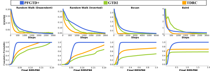
Figure 2: Top row: Learning curves in classic RL domains. The curves for TDC and GTD2 are with their respective best hyperparameter combinations after a grid search (see Section F.1). Each curve shows the average RMSPBE over 200 runs. Standard errors are plotted but are vanishingly small. Bottom row: CDF plots of the final RMSPBE for each algorithm. Uniform sampling to select hyperparameters of the baselines on each of 5,000 runs. In each plot a point $(x,y)$ means that $y$ proportion of the runs resulted in a final $\text{RMSPBE}\leq x$.

PFGTD+ takes advantage of sparsity when the coordinate-wise bound is the better of the two, while still guaranteeing the dimension-free bound of the PF subroutine. Notice that we still retain a dimension-dependent penalty as a constant factor in either case, so the bound is never truly dimension-free, even when $R_{T}^{\text{PF}}\leq R_{T}^{\text{CW-PF}}$. We might instead think of the algorithm as “almost dimension-free”, in the sense that the undesireable dimension penalty is only on constant terms. Achieving both the dimension-free and coordinate-wise bounds simultaneously has been recently achieved using a generic combiner algorithm (Bhaskara et al., 2020), but requires solving a linear optimization problem on each step. Instead, our approach trades this (potentially large) computational overhead for a transient dimension penalty. Our experiments suggest that this penalty has little effect, with PFGTD+ performing similarly to whichever algorithm happens to work best in each problem.

4 Experiments

We test the performance of our algorithms in two main settings: (1) classic MDPs used to study learning stability under function approximation and off-policy updates, and (2) a prediction problem on data from a mobile robot, involving an immense number of sensory inputs, all of varying scales and levels of noise corruption.

As our parameter-free algorithms utilize the saddle-point formulation of GTD2 (Liu et al., 2018), GTD2 is our primary baseline. A favourable comparison between our parameter-free methods and a well-tuned GTD2 baseline would indicate that our algorithms can be used as a drop-in replacement for GTD2, with similar guarantees and performance in practice, yet without parameter tuning. We additionally include TDRC (Ghiassian et al., 2020), a recently proposed extension of TDC which is currently the state-of-the-art gradient TD method. Together with GTD2, these two baselines captured the full range of performance of all other tested baselines, so we defer additional baselines to Section F.2.

Our aim in these experiments is not to show that our algorithms outperform the baselines — this would be expecting too much, as parameter-free methods achieve optimal rates only up to logarithmic terms. Our goal is rather to show that our methods can achieve performance reasonably comparable to that of tuned baselines, with no tuning at all. This result would indicate both a favourable performance-computation trade-off and robustness to unknown conditions.

4.1 Classic RL Problems

We test our algorithms on three classic MDPs: Baird’s counterexample (Baird, 1995), Boyan’s chain (Boyan, 2002), and a five-state random walk MDP (Sutton et al., 2009). In Baird’s counterexample, the combination of large importance sampling ratios and pathogenic generalization from the features leads TD to diverge. Boyan’s chain poses similar generalization difficulties, but is an on-policy problem. The random walk MDP has been used extensively in prior benchmarks of gradient TD methods; we apply it with two difficult feature sets: the inverted and dependent feature sets. Each of these problems are all well-known in our problem setting so we defer their details to Section F.1.

Figure 4 (top row) plots performance over time, measured in terms of root mean-square projected Bellman error (RMSPBE), which can be computed exactly in these problems. From these plots we can glean a couple of trends. First, even in comparison to extensively tuned baselines, our parameter-free algorithms still achieve comparable levels of error, without any hyperparameter tuning. Second, we observe that PFGTD+ initially converges more slowly than the baselines, consistent with the logarithmic penalty we pay in our regret bounds. Nevertheless, this penalty does not hamper asymptotic convergence, and indeed for all four plots, the RMSPBE of PFGTD+ is equal to or comparable to the RMSPBEs of the baselines at the right end of the $x$-axis.

To measure the performance in the absence of a priori information about optimal hyperparameters, we use cumulative distribution function (CDF) plots. Given an algorithm and a method of choosing hyperparameters on each run, CDF plots treat each run as a draw from a random variable that represents that algorithm’s performance, plotting the resulting empirical CDF. For a given curve, a point $(x,y)$ means that $y$ proportion of the runs resulted in a final RMSPBE $\leq$ $x$. On each of 5,000 runs, we select the step-size of the baseline algorithms uniformly randomly, reflecting a situation in which relevant information is missing prior to running the algorithm. These plots also illustrate a work-performance trade off: algorithms which require substantial tuning to achieve good performance are sensitive to the tuned parameter, and will thus have a higher proportion of poorly performing runs when the parameter is chosen randomly.

The CDF plots for each of the classic RL problems are shown in Figure 4 (bottom row). A larger proportion of the runs of our parameter-free methods achieve a low final RMSPBE compared to the baselines. For example, on Baird’s counterexample, about 90% of the runs of PFGTD+ achieve an error $\leq$ 0.5, while only at most about 60% of the runs of GTD2 and TDRC achieve an error $\leq$ 2. The reason for this is that achieving the optimal rates for the baselines depend upon hyperparameter search, whose difficulty is captured by the area under the CDF curve. Indeed, error values $x$ such that $\int_{0}^{x}\text{CDF}(z)dz$ is small are values that were encountered infrequently, indicating that the parameters to achieve such error are difficult to find. On the other hand, the CDF plots demonstrate that PFGTD+ is less likely to achieve error as low as the very best runs of the baselines. Yet, the PFGTD+ CDF curves tend to rise sharply near $x=0$ before plateauing at $y=1$, indicating that PFGTD+ reliably achieves performance not far off from the optimally-tuned baselines with no hyperparameter tuning whatsoever.

Finally, the bar plot depicted in-line shows the average area under the RMSPBE curve over 200 runs $\pm$ 1 standard error in each of the classic RL problems. The measurements are normalized by the performance of PFGTD+ to provide a similar scale across problems. We observe that PFGTD+ tends to perform at least as well as the best of PFGTD and CW-PFGTD. Furthermore, with the exception of Boyan’s chain, we actually see a slight improvement over both components, suggesting that the iterate adding approach is itself beneficial.

4.2 Large-scale Prediction

In practical problems, agents can face a large array of signals, each of varying magnitudes, signal-to-noise ratios, and degrees of non-stationarity. A learning rate that is optimal for one signal is thus unlikely to perform well for another signal, yet tuning learning rates for every single sensor can be prohibitively expensive, forcing us to compromise across all sensors. We test performance under such conditions by recreating the robot nexting experiment of Modayil et al. (2014), in which a mobile robot interacts with the environment according to a fixed behaviour policy making predictions about future sensor readings along the way. We predict the future returns of each of the 53 sensor readings at a discount rate of $\gamma=0.9875$, corresponding to approximately 80 steps into the future. The features are constructed from the robot’s sensor readings using the same sparse representation as the original work. Performance was measured in terms of the symmetric mean absolute percentage error (SMAPE). For a given sensor $s$, the SMAPE over the first $T$ samples is defined as $\text{SMAPE}(T,s)\overset{\text{def}}{=}\frac{1}{T}\sum_{t=1}^{T}\frac{|\hat{v}^{(s)}(S_{t})-G_{t}^{(s)}|}{|G_{t}^{(s)}|+|\hat{v}^{(s)}(S_{t})|}.$ SMAPE is bounded in [0, 1] and scale-independent, allowing the comparison of errors across different sensors.

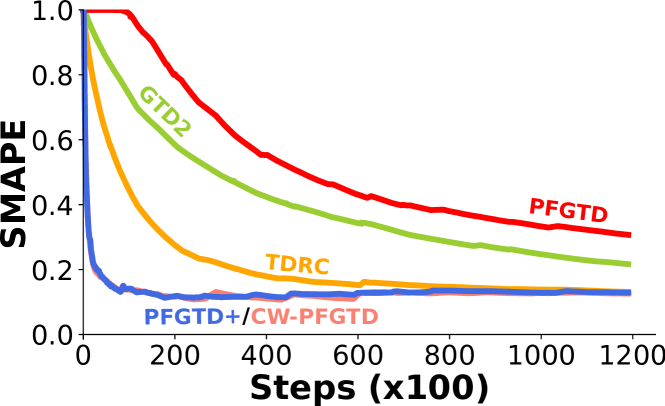
Figure 3: The median symmetric mean absolute percentage error (SMAPE) across all 53 sensors in the large-scale prediction problem. The SMAPE measures prediction accuracy compared with the ideal predictions (the true returns), computed offline using all future data. Baseline algorithms are tuned via grid search (see Section F.1).

The results on this task are shown in Figure 3. As with the previous set of experiments, PFGTD+ achieves comparable or better final error to the baselines. Notably, despite tuning both GTD2 and TDRC, neither algorithm is able to match the convergence rate of PFGTD+ and CW-PFGTD. In this high-dimensional prediction problem, no single step-size will perform well across all sensors due to the variation in scale and noise levels between the different sensors. Our algorithms obviate such concerns by adapting to both the sequence of gradients and the unknown saddle-point, and doing so without requiring knowledge of problem-dependent constants. The result also highlights the importance of the combined approach of PFGTD+ — the PFGTD algorithm leaves considerable performance gains on the table by being unable to adapt to sparsity.

5 Conclusion

In this paper, we bring to bear recent work in parameter-free online learning to policy evaluation. Using the Saddle-point formulation of GTD2 and the framework of parameter-free online learning through coin-betting, we derive algorithms with robust guarantees and performance similar to that of tuned baselines, without any parameter tuning. While tuned baselines are capable of achieving lower error overall, the computational expense is large and may need to be repeated every time a distributional shift occurs in the environment.

There are several interesting directions for future work. First, two-timescale algorithms such as TDC and TDRC are well-known to be more performant than the algorithms derived from the Saddle-point perspective (Sutton et al., 2009; Ghiassian et al., 2020). Developing parameter-free variants of these algorithms is less straightforward, but could have even greater practical utility. Second, as noted in Section 3.3, our proposed algorithm never quite achieves both the dimension-free and AdaGrad regret bound simultaneously. Recent work has achieved such bounds with a generic combiner algorithm (Bhaskara et al., 2020), but can require non-trivial additional computation on each step. It remains to be seen whether removing the penalty in our approach is worth the extra computation. Finally, future work will investigate extensions of our approach to the control setting.

Appendix A Saddle-point to OLO Reduction

In this section we show how a convex-concave saddle-point problem can be reduced to a constrained OLO problem. This reduction is included for completeness, but similar arguments can be seen in a variety of works which apply Mirror Descent or other “proximal”-type algorithms to saddle-point problems (Nemirovski et al., 2009; Mertikopoulos et al., 2018; Juditsky et al., 2019).

Let $\Theta\subset\mathbb{R}^{m}$ and $\mathcal{Y}\subset\mathbb{R}^{n}$ be compact convex sets and let $L:\Theta\times\mathcal{Y}\rightarrow\mathbb{R}$ be a continuous map such that $L(\cdot,y)$ is convex and $L(\theta,\cdot)$ concave. We are interested in finding the saddle point of $L$, i.e. , an $(\theta^{*},y^{*})\in\Theta\times\mathcal{Y}$ such that

$$L(\theta^{*},y^{*})=\inf_{\theta\in\Theta}\sup_{y\in\mathcal{Y}}L(\theta,y)=\sup_{y\in\mathcal{Y}}\inf_{\theta\in\Theta}L(\theta,y).$$ (8)

With our assumptions on $\Theta$ and $\mathcal{Y}$ the existence of such a point $(x^{*},y^{*})\in\mathcal{Z}$ follows from Sion’s Minimax Theorem (Boyd & Vandenberghe, 2004). We measure the quality of a candidate solution $z=(\theta,y)$ via the Duality gap:

$$\max_{y^{*}\in\mathcal{Y}}L(\theta,y^{*})-\min_{\theta^{*}\in\Theta}L(\theta^{*},y)$$ (9)

It can be shown that this quantity is non-negative, and any $(\theta,y)\in\Theta\times\mathcal{Y}$ for which $\max_{y^{*}\in\mathcal{Y}}L(\theta,y^{*})-\min_{\theta^{*}\in\Theta}L(\theta^{*},y)=0$ must be a saddle-point of SP problem 3 (shown as an aside in Box A). Finally, it can be shown that the saddle point of our saddle point problem, Equation 3, corresponds to a minimizer of the MSPBE (or NEU) (Liu et al., 2018).

Next, we show that this duality gap can be bounded in terms of the regrets incurred by two separate online learning algorithms. Consider points $\overline{\theta}_{T}=\frac{1}{T}\sum_{t=1}^{T}\theta_{t}$ and $\overline{y}_{T}=\sum_{t=1}^{T}y_{t}$ for sequences with $\theta_{t}\in\Theta$ and $y_{t}\in\mathcal{Y}$ chosen by online learning algorithms $\mathcal{A}_{\Theta}$ and $\mathcal{A}_{\mathcal{Y}}$ respectively. Let $(\theta^{*},y^{*})\in\Theta\times\mathcal{Y}$. Using the convexity of $L$ in its first argument and $-L$ in its second argument, we can write

$$L(\overline{\theta}_{T},y^{*})-L(\theta^{*},\overline{y}_{T})$$

$$\quad\leq\frac{1}{T}\sum\limits_{t=1}^{T}L(\theta_{t},y^{*})-\frac{1}{T}\sum_{t=1}^{T}L(\theta^{*},y_{t})$$

$$\quad=\frac{\sum\limits_{t=1}^{T}L(\theta_{t},y^{*})-L(\theta^{*},y_{t})}{T}$$

$$\quad=\frac{\sum\limits_{t=1}^{T}L(\theta_{t},y^{*})-L(\theta_{t},y_{t})+L(\theta_{t},y_{t})-L(\theta^{*},y_{t})}{T}$$

$$\quad\overset{(a)}{\leq}\frac{\sum\limits_{t=1}^{T}\langle g_{t}^{y},y_{t}-y^{*}\rangle+\sum\limits_{t=1}^{T}\langle g_{t}^{\theta},\theta_{t}-\theta^{*}\rangle}{T}$$

where $(a)$ defined $g_{t}^{\theta}\in\partial_{\theta}L(\theta_{t},y_{t})$, $g_{t}^{y}\in-\partial_{y}L(\theta_{t},y_{t})$ and used of convexity of $L(\cdot,y_{t})$ and $-L(\theta_{t},\cdot)$. Observe that the quantities in the last line can be seen as average regrets $\frac{1}{T}R_{T}^{\mathcal{A}_{\Theta}}$ and $\frac{1}{T}R_{T}^{\mathcal{A}_{\mathcal{Y}}}$ of two algorithms $\mathcal{A}_{\Theta}$ and $\mathcal{A}_{\mathcal{Y}}$ played against the loss sequences $\theta\mapsto\langle g_{t}^{\theta},\theta\rangle$ and $y\mapsto\langle g_{t}^{y},y\rangle$ respectively. Thus we can ensure that the duality gap approaches zero by providing OLO algorithms $\mathcal{A}_{\Theta}$ and $\mathcal{A}_{\mathcal{Y}}$ which guarantee sublinear regret. Thus we have the following “Folk Theorem”, commonly used to reduce min-max problems to separate OLO problems:

Proposition 4 (Folk Theorem)

Let $\mathcal{A}_{\Theta}$ and $\mathcal{A}_{\mathcal{Y}}$ be online learning algorithms with compact and convex domains $\Theta$ and $\mathcal{Y}$ respectively. Let $R_{T}^{\mathcal{A}_{\Theta}}(\theta^{*})$ and $R_{T}^{\mathcal{A}_{\mathcal{Y}}}(y^{*})$ denote the linear regret of algorithms $\mathcal{A}_{\Theta}$ and $\mathcal{A}_{\mathcal{Y}}$. Then for any $(\theta^{*},y^{*})\in\Theta\times\mathcal{Y}$,

$$L\Big{(}\overline{\theta}_{T},y^{*}\Big{)}-L\Big{(}\theta^{*},\overline{y}_{T}\Big{)}\leq\frac{R_{T}^{\mathcal{A}_{\Theta}}(\theta^{*})+R_{T}^{\mathcal{A}_{\mathcal{Y}}}(y^{*})}{T}.$$

Note that we can equivalently state the above in terms of the regret of a single algorithm with domain $\mathcal{Z}=\Theta\times\mathcal{Y}$. Namely, by letting $g_{t}\overset{\text{def}}{=}(g_{t}^{\theta},g_{t}^{y})$, $z_{t}\overset{\text{def}}{=}(\theta_{t},y_{t})$, and $z^{*}=(\theta^{*},y^{*})$, we can write

$$L\Big{(}\overline{\theta}_{T},y^{*}\Big{)}-L\Big{(}\theta^{*},\overline{y}_{T}\Big{)} \leq\frac{\sum\limits_{t=1}^{T}\langle g_{t},z_{t}-z^{*}\rangle}{T}=\frac{R_{T}^{\mathcal{A}_{\mathcal{Z}}}(z^{*})}{T}.$$

This form will sometimes be a bit easier to work with due to requiring less notation.

The Folk Theorem extends straight-forwardly to the stochastic setting using a simple online-to-batch conversion (Cesa-Bianchi et al., 2004; Orabona, 2019) argument.

Proposition 5

Let $\mathcal{A}_{\Theta}$ and $\mathcal{A}_{\mathcal{Y}}$ be online learning algorithms with domains $\Theta$ and $\mathcal{Y}$ respectively. Suppose $({\hat{g}}_{t}^{\theta})_{t=1}^{T}$ and $({\hat{g}}_{t}^{y})_{t=1}^{T}$ are sequences satisfying $\mathbb{E}\left[\hat{g}_{t}^{\theta}|\theta_{t},y_{t}\right]\in\partial_{\theta}L(\theta_{t},y_{t})$ and $\mathbb{E}\left[\hat{g}_{t}^{y}|\theta_{t},y_{t}\right]\in-\partial_{y}L(\theta_{t},y_{t})$ for all $t\in[T]$. Then for any $(\theta^{*},y^{*})\in\Theta\times\mathcal{Y}$,

$$\mathbb{E}\left[L\Big{(}\overline{\theta}_{T},y^{*}\Big{)}-L\Big{(}\theta^{*},\overline{y}_{T}\Big{)}\right]\leq\frac{\mathbb{E}\left[R_{T}^{\mathcal{A}_{\Theta}}(\theta^{*})+R_{T}^{\mathcal{A}_{\mathcal{Y}}}(y^{*})\right]}{T},$$

where $R_{T}^{\mathcal{A}_{\Theta}}(\theta^{*})=\sum_{t=1}^{T}\langle\hat{g}_{t}^{\theta},\theta_{t}-\theta^{*}\rangle$ and $R_{T}^{\mathcal{A}_{\mathcal{Y}}}(y^{*})=\sum_{t=1}^{T}\langle\hat{g}_{t}^{y},y_{t}-y^{*}\rangle$.

The proof follows easily by using convexity followed by the tower rule:

$$\mathbb{E}\left[L(\overline{\theta}_{T},y^{*})-L(\theta^{*},\overline{y}_{T})\right]$$

$$\qquad\leq\frac{\mathbb{E}\left[\sum_{t=1}^{T}\langle g_{t}^{\theta},\theta_{t}-\theta^{*}\rangle+\sum_{t=1}^{T}\langle g_{t}^{y},y_{t}-y^{*}\rangle\right]}{T}$$

$$\qquad=\frac{\mathbb{E}\left[\sum_{t=1}^{T}\langle\hat{g}_{t}^{\theta},\theta_{t}-\theta^{*}\rangle+\sum_{t=1}^{T}\langle\hat{g}_{t}^{y},y_{t}-y^{*}\rangle\right]}{T}$$

$$\qquad=\mathbb{E}\left[\frac{R_{T}^{\mathcal{A}_{\Theta}}(\theta^{*})+R_{T}^{\mathcal{A}_{\mathcal{Y}}}(y^{*})}{T}\right]$$

Using this simple reduction, we can see that our problem of minimizing the MSPBE (or NEU) can be reduced to two separate OLO problems; if we can find algorithms which guarantee sublinear regret on the stochastic linear losses ${\hat{g}}_{t}^{\theta}$ and ${\hat{g}}_{t}^{y}$ given by Equations 5, then the duality gap (and thus MSPBE) will approach zero in expectation $T\rightarrow\infty$. In the following sections we can thus focus our attention on constructing OLO algorithms with various desirable properties.

Appendix B Proof of Theorem 1

The theorem is repeated below for for convenience.

See 1

Proof: Let ${\hat{g}}_{t}^{\theta}$ and ${\hat{g}}_{t}^{y}$ be such that $\mathbb{E}\left[{\hat{g}}_{t}^{\theta}|\theta_{t},y_{t}\right]=g_{t}^{\theta}\in\partial_{\theta}L(\theta_{t},y_{t})$ and $\mathbb{E}\left[{\hat{g}}_{t}^{y}|\theta_{t},y_{t}\right]=g_{t}^{y}\in\partial_{y}L(\theta_{t},y_{t})$ respectively. Further, endow $\Theta\times\mathcal{Y}$ with norm $\|z\|=\|(\theta,y)\|=\sqrt{\|\theta\|^{2}+\|y\|^{2}}$ and define $z_{t}\overset{\text{def}}{=}(\theta_{t},y_{t})$ and ${\hat{g}}_{t}\overset{\text{def}}{=}({\hat{g}}_{t}^{\theta},-{\hat{g}}_{t}^{y})$. Following Appendix A we have that for saddle-point $z^{*}\overset{\text{def}}{=}(\theta^{*},y^{*})\in\Theta\times\mathcal{Y}$,

$$\mathbb{E}\left[L(\overline{\theta}_{T},y^{*})-L(\theta^{*},\overline{y}_{T})\right]\leq\mathbb{E}\left[\frac{R_{T}^{\mathcal{A}}(z^{*})}{T}\right]$$

$$\qquad\overset{(a)}{\leq}\mathbb{E}\left[\frac{A_{T}(z^{*})+B_{T}(z^{*})\sqrt{\sum_{t=1}^{T}\|{\hat{g}}_{t}\|^{2}}}{T}\right]$$

$$\qquad\overset{(b)}{\leq}\frac{A_{T}(z^{*})+B_{T}(z^{*})\sqrt{\sum_{t=1}^{T}\mathbb{E}\left[\|{\hat{g}}_{t}\|^{2}\right]}}{T}$$ (10)

where $(a)$ used the regret guarantee of $\mathcal{A}$ applied to the loss sequence $z_{t}\mapsto\langle{\hat{g}}_{t},z_{t}\rangle$, and $(b)$ applied Jensen’s inequality w.r.t the function $x\mapsto\sqrt{x}$. As shown in Box B, the terms $\mathbb{E}\left[\|{\hat{g}}_{t}\|^{2}\right]$ are bounded above by $G^{2}\overset{\text{def}}{=}D^{2}\Big{(}2\|A\|+\lambda_{\max}(M)+\frac{\sigma+\|b\|}{D}\Big{)}^{2}$, so (10) becomes

$$\mathbb{E}\left[\frac{L(\overline{\theta}_{T},y^{*})-L(\theta^{*},\overline{y}_{T})}{T}\right]$$

$$\qquad\leq\frac{A_{T}(z^{*})+B_{T}(z^{*})\sqrt{TG^{2}}}{T}$$

$$\qquad=\frac{A_{T}(z^{*})}{T}+\frac{B_{T}(z^{*})D\Big{(}2\|A\|+\lambda+\frac{\sigma+\|b\|}{D}\Big{)}}{\sqrt{T}},$$

with $\lambda=\lambda_{\max}(M)$.

For the high probability statement, define $G^{2}$ as before and assume the following stronger assumption holds:

$$\mathbb{E}\left[\exp\left(\frac{\|{\hat{g}}_{t}\|^{2}}{G^{2}}\right)\right]\leq\exp\left(1\right).$$ (11)

Similarly to the expectation bound, we begin by bounding the duality gap by the regret of $\mathcal{A}$:

$$L(\overline{\theta}_{T},y^{*})-L(\theta^{*},\overline{y}_{T})\leq\frac{\sum_{t=1}^{T}\langle g_{t},z_{t}-z^{*}\rangle}{T}$$

$$\qquad=\frac{\sum_{t=1}^{T}\langle{\hat{g}}_{t},z_{t}-z^{*}\rangle+\langle g_{t}-{\hat{g}}_{t},z_{t}-z^{*}\rangle}{T}$$

$$\qquad=\underbrace{\frac{\sum_{t=1}^{T}\langle{\hat{g}}_{t},z_{t}-z^{*}\rangle}{T}}_{\leavevmode\hbox to6.09pt{\vbox to6.09pt{\text{[drawing]}}}}+\underbrace{\frac{\sum_{t=1}^{T}\langle g_{t}-{\hat{g}}_{t},z_{t}-z^{*}\rangle}{T}}_{\leavevmode\hbox to6.09pt{\vbox to6.09pt{\text{[drawing]}}}}$$

Bounding Using the regret guarantee of $\mathcal{A}$, we again have

$$\frac{\sum_{t=1}^{T}\langle{\hat{g}}_{t},z_{t}-z^{*}\rangle}{T}\leq\frac{A_{T}(z^{*})+B_{T}(z^{*})\sqrt{\sum_{t=1}^{T}\|{\hat{g}}_{t}\|^{2}_{*}}}{T},$$

where $A_{T}(\cdot)$ and $B_{T}(\cdot)$ are deterministic non-negative functions. To bound this term we can use a Cramer-Chernoff-style argument. Let $\varepsilon>0$, and consider $\mathbb{P}\left\{\sqrt{\sum_{t=1}^{T}\|{\hat{g}}_{t}\|^{2}}>\varepsilon\right\}$. Letting $\eta>0$ be a variable to be sorted out later, we have

$$\mathbb{P}\left\{\sqrt{\sum_{t=1}^{T}\|{\hat{g}}_{t}\|^{2}}\geq\varepsilon\right\}$$

$$=\mathbb{P}\left\{\exp\left(\eta\sqrt{\sum_{t=1}^{T}\|{\hat{g}}_{t}\|^{2}}\right)\geq\exp\left(\eta\varepsilon\right)\right\}$$

$$\leq\exp\left(-\eta\varepsilon\right)\mathbb{E}\left[\exp\left(\eta\sqrt{\sum_{t=1}^{T}\|{\hat{g}}_{t}\|^{2}}\right)\right],$$

with the last line resulting from Markov’s inequality. Next, we notice that the second term bears some resemblance to the terms in the light-tailed assumption (11) which are bounded above by $\exp\left(1\right)$, so a natural approach would be to try to set $\eta$ to expose terms of this form. Indeed, as shown in Box B, if we set $\eta=\frac{1}{\sqrt{T}G}$, then

$$\exp\left(-\eta\varepsilon\right)\mathbb{E}\left[\exp\left(\eta\sqrt{\sum_{t=1}^{T}\|{\hat{g}}_{t}\|^{2}}\right)\right]$$

$$\qquad\leq\exp\left(\frac{-\varepsilon}{\sqrt{T}G}+2\right),$$

and so the deviation bound for is

$$\mathbb{P}\left\{\frac{A_{T}(z^{*})+B_{T}(z^{*})\sqrt{\sum_{t=1}^{T}\|{\hat{g}}_{t}\|^{2}}}{T}\geq\frac{A_{T}(z^{*})+B_{T}^{*}(z^{*})\varepsilon}{T}\right\}$$

$$\qquad\leq\exp\left(\frac{-\varepsilon}{\sqrt{T}G}+2\right)$$ (12)

Bounding This term requires some additional trickery but the basic idea is still the same. As before, introduce a variable $\eta>0$ to be set later and let $\varepsilon>0$. Then

$$\mathbb{P}\left\{\sum_{t=1}^{T}\langle g_{t}-{\hat{g}}_{t},z_{t}-z^{*}\rangle\geq\varepsilon\right\}$$

$$=\mathbb{P}\left\{\exp\left(\eta\sum_{t=1}^{T}\langle g_{t}-{\hat{g}}_{t},z_{t}-z^{*}\rangle\right)\geq\exp\left(\eta\varepsilon\right)\right\}$$

$$\leq\exp\left(-\eta\varepsilon\right)\mathbb{E}\left[\exp\left(\eta\sum_{t=1}^{T}\langle g_{t}-{\hat{g}}_{t},z_{t}-z^{*}\rangle\right)\right].$$ (13)

Next, define the following short-hand notations

$$\xi_{t} \overset{\text{def}}{=}\langle g_{t}-{\hat{g}}_{t},z_{t}-z^{*}\rangle$$

$$\mathcal{F}_{t} \overset{\text{def}}{=}(s_{\tau},a_{\tau},r_{\tau},s_{\tau}^{\prime},\theta_{\tau},y_{\tau})_{\tau=1}^{t}$$

and observe that $\xi_{t}$ is a deterministic function of $\mathcal{F}_{t}$, and that $\mathbb{E}\left[\xi_{t}|\mathcal{F}_{t-1}\right]=0$. Thus, we can write

$$\mathbb{E}\left[\exp\left(\eta\sum_{t=1}^{T}\langle g_{t}-{\hat{g}}_{t},z_{t}-z^{*}\rangle\right)\right]$$

$$\qquad=\mathbb{E}\left[\exp\left(\eta\sum_{t=1}^{T}\xi_{t}\right)\right]$$

$$\qquad=\mathbb{E}\left[\mathbb{E}\left[\exp\left(\eta\sum_{t=1}^{T}\xi_{t}\right)\Big{|}\mathcal{F}_{T-1}\right]\right]$$

$$\qquad=\mathbb{E}\left[\exp\left(\eta\sum_{t=1}^{T-1}\xi_{t}\right)\mathbb{E}\left[\exp\left(\eta\xi_{T}\right)\Big{|}\mathcal{F}_{T-1}\right]\right].$$

As we show in Box B, for each $t$ we have that $\mathbb{E}\left[\exp\left(\eta\xi_{t}\right)\Big{|}\mathcal{F}_{t-1}\right]\leq\exp\left(4\eta^{2}G^{2}D^{2}\right)$, so

$$\mathbb{E}\left[\exp\left(\eta\sum_{t=1}^{T-1}\xi_{t}\right)\mathbb{E}\left[\exp\left(\eta\xi_{T}\right)\Big{|}\mathcal{F}_{T-1}\right]\right]$$

$$\leq\mathbb{E}\left[\exp\left(\eta\sum_{t=1}^{T-1}\xi_{t}\right)\exp\left(4\eta^{2}G^{2}D^{2}\right)\right]$$

$$\leq\ldots\leq\exp\left(4\eta^{2}G^{2}D^{2}T\right).$$

Plugging this back into (13) gives us

$$\mathbb{P}\left\{\sum_{t=1}^{T}\langle g_{t}-{\hat{g}}_{t},z_{t}-z^{*}\rangle\geq\varepsilon\right\}$$

$$\qquad\leq\exp\left(-\eta\varepsilon+4\eta^{2}G^{2}D^{2}T\right)=\exp\left(\frac{-\varepsilon^{2}}{16TG^{2}D^{2}}\right),$$

where in the final equality we set $\eta=\frac{\varepsilon}{8G^{2}D^{2}T}$ to balance the terms. Thus for we have a deviation bound of

$$\mathbb{P}\left\{\frac{\sum_{t=1}^{T}\langle g_{t}-{\hat{g}}_{t},z_{t}-z^{*}\rangle}{T}>\frac{\varepsilon}{T}\right\}\leq\exp\left(\frac{-\varepsilon^{2}}{16TG^{2}D^{2}}\right).$$

With bounds for and in hand, we have that for any $\varepsilon_{1},\varepsilon_{2}>0$,

$$\mathbb{P}\left\{\leavevmode\hbox to8.53pt{\vbox to8.53pt{\text{[drawing]}}}+\leavevmode\hbox to8.53pt{\vbox to8.53pt{\text{[drawing]}}}\geq\frac{A_{T}(z^{*})+B_{T}(z^{*})\varepsilon_{1}+\varepsilon_{2}}{T}\right\}$$

$$\qquad\leq\exp\left(\frac{-\varepsilon_{1}}{\sqrt{T}G}+2\right)+\exp\left(\frac{-\varepsilon_{2}^{2}}{16TG^{2}D^{2}}\right)$$

$$\qquad\leq 2\exp\left(\frac{-\varepsilon_{2}^{2}}{16TG^{2}D^{2}}+1\right)$$

where in the last line we used $\exp\left(\frac{-\varepsilon_{2}^{2}}{16TG^{2}D^{2}}\right)\leq\exp\left(\frac{-\varepsilon_{2}^{2}}{16TG^{2}D^{2}}+1\right)$ and then chose $\varepsilon_{1}=\sqrt{T}G\Big{(}1+\frac{\varepsilon_{2}^{2}}{16TG^{2}D^{2}}\Big{)}$. Equivalently, letting $\delta\overset{\text{def}}{=}2\exp\left(\frac{-\varepsilon_{2}^{2}}{16TG^{2}D^{2}}+1\right)$, we solve for $\varepsilon_{2}$ to get $\varepsilon_{2}=4D\sqrt{1+\log\left(\frac{2}{\delta}\right)}\sqrt{T}G$, and conclude that with probability at least $1-\delta$,

$$\max_{y^{*}\in\mathcal{Y}}L(\overline{\theta}_{T},y^{*})-\min_{\theta^{*}\in\Theta}L(\theta^{*},\overline{y}_{T})$$

$$\qquad\leq\frac{A_{T}(z^{*})+B_{T}(z^{*})\sqrt{\sum_{t=1}^{T}\|{\hat{g}}_{t}\|^{2}}+\sum_{t=1}^{T}\xi_{t}}{T}$$

$$\qquad\leq\frac{A_{T}(z^{*})}{T}+\frac{B_{T}(z^{*})\Big{(}1+\log\left(\frac{2}{\delta}\right)\Big{)}G}{\sqrt{T}}$$

$$\qquad\qquad\qquad+\frac{4D\sqrt{1+\log\left(\frac{2}{\delta}\right)}G}{\sqrt{T}}$$

The proof is then completed by using $a+b\leq 2\max\left\{a,b\right\}$ and substituting the lipschitz bound $G$ as before.

Appendix C Coin-betting and Black-box Reductions

In this section we give a brief overview of the key ideas and algorithms from the online learning literature used in this paper.

Our primary interest in this paper is avoiding having to tune a step-size parameter. Interestingly, it turns out that achieving this goal is related to a particular type of adaptivity — adaptivity to the norm of any given comparator point $u$ — manifesting in regret bounds of the form $O\Big{(}\|u\|\sqrt{\sum_{t=1}^{T}\|g_{t}\|^{2}}\Big{)}$. To see this, one can imagine running online gradient descent (OGD) with a fixed step-size $\eta$, and ask what the optimal choice of fixed choice $\eta$ would be in hindsight — if we could choose or approximate this optimal $\eta$ in advance, no tuning would be necessary. Following standard analysis (Orabona, 2019, Theorem 2.13), one can derive that the regret of OGD with a fixed step-size is bounded as $R_{T}(u)\leq\frac{\|u\|^{2}}{2\eta}+\frac{\eta}{2}\sum_{t=1}^{T}\|g_{t}\|^{2}$, from which the optimal bound $R_{T}(u)\leq\|u\|\sqrt{\sum_{t=1}^{T}\|g_{t}\|^{2}}$ can be derived by choosing $\eta^{*}=\frac{\|u\|}{\sqrt{\sum_{t=1}^{T}\|g_{t}\|^{2}}}$. Of course, we could never actually select this $\eta^{*}$ in practice as it requires knowing all the future subgradients $g_{t}$ as well as the norm of the unknown comparator point $u$. In fact one can show that it’s actually impossible to achieve this $O\Big{(}\|u\|\sqrt{\sum_{t=1}^{T}\|g_{t}\|^{2}}\Big{)}$ bound without knowing $u$ in advance (Orabona, 2019, Chapter 5). However, several recent works can make guarantees of this form up to log factors, particularly those operating in the coin-betting framework (Cutkosky & Orabona, 2018; Orabona & Pál, 2016).

In the coin-betting framework, the objective of guaranteeing low regret $R_{T}=\sum_{t=1}^{T}\langle g_{t},x_{t}-u\rangle$ is re-cast as a betting problem in which the objective is to guarantee high wealth, $W_{T}\overset{\text{def}}{=}W_{0}-\sum_{t=1}^{T}\langle g_{t},x_{t}\rangle$, starting from some initial endowment of $W_{0}$. Concretely, in the 1-dimensional OLO case, at each time $t\in[T]$ the learner places a bet $x_{t}=\beta_{t}W_{t-1}$ — corresponding to some (signed) fraction $\beta_{t}\in[-1,1]$ of their current wealth $W_{t-1}$ — on the outcome of a continuous-valued “coin” $-g_{t}\in[-1,1]$. The learner either wins (or loses) the amount $-g_{t}x_{t}$, and their wealth becomes $W_{t}=W_{t-1}-g_{t}x_{t}=W_{t-1}(1-\beta_{t}g_{t})$. The key idea is that guaranteeing a lower-bound on wealth corresponds to guaranteeing an upper-bound on regret: letting $F$ be a convex potential function and $F^{*}$ its Fenchel conjugate, it holds that (McMahan & Orabona, 2014)

$$W_{T}\geq F\Big{(}\sum_{t=1}^{T}-g_{t}\Big{)}-W_{0}\Longleftrightarrow/R_{T}(u)\leq F^{*}(u)+W_{0}.$$

The key observation here is that designing a regret-minimizing algorithm which is adaptive w.r.t the comparator $u$ — the key property of parameter-free algorithms — is equivalent to designing a betting strategy which is adaptive w.r.t $\sum_{t=1}^{T}-g_{t}$. Notably, it is much easier to design algorithms which are adaptive to this latter quantity because it can be directly observed and measured by the learner.

In this paper, we employ a betting strategy based on the Online Newton Step Coin-betting algorithm of Cutkosky & Orabona (2018, Algorithm 1). The basic idea is as follows: at any time $t$ we can express our accumulated wealth as a function of our chosen betting fractions, $W_{t}=W_{t-1}\Big{(}1-g_{t}\beta_{t}\Big{)}=W_{0}\prod_{s=1}^{t-1}\Big{(}1-g_{s}\beta_{s}\Big{)}$, and we can consider how much more wealth could have been attained if we had just used the best fixed betting fraction in hindsight:

$$\frac{\max_{\beta^{*}\in[-1,1]}\prod_{s=1}^{t-1}\Big{(}1-g_{t}\beta^{*}\Big{)}}{\prod_{s=1}\Big{(}1-g_{t}\beta_{t}\Big{)}}.$$

Equivalently, by taking the logarithm of this quantity we’re interested in the difference $\max_{\beta\in[-1,1]}\sum_{s=1}^{t}\log\left(1-g_{t}\beta^{*}\right)-\sum_{s=1}^{t}\log\left(1-g_{t}\beta_{t}\right)$, which we observe is the regret of our choices $\beta_{t}$ on the sequence of loss functions $\ell_{t}(\beta)\overset{\text{def}}{=}-\log\left(1-g_{t}\beta\right)$. We can therefore try to learn about the optimal betting fraction $\beta^{*}$ by applying an online learning algorithm to this loss sequence. Luckily, these loss functions happen to have nice curvature properties which enable us to use the efficient Online Newton Step (ONS) algorithm (Hazan et al., 2007) — this means that we’ll be able to converge to good betting fractions very quickly and obtain high wealth. In fact, this strategy will give us exactly the regret we’re looking for, $R_{T}(u)=\widetilde{O}\Big{(}|u|\sqrt{\sum_{t=1}^{T}|g_{t}|^{2}}\Big{)}$, and the algorithm can be extended to higher dimensions to achieve a bound of the same form using either the black-box reduction of Cutkosky & Orabona (2018, Algorithm 2), or by applying the betting strategy separately in each dimension, resulting in a coordinate-wise, AdaGrad-style algorithm.

However, for our purposes the approach described above is a bit unsatisfying as it requires knowing a Lipschitz bound on the gradients a priori. Recall that in the coin-betting framework, the learner bets $x_{t+1}=\beta_{t+1}W_{t}$, and as a result the wealth becomes $W_{t+1}=W_{t}(1-\beta_{t+1}g_{t+1})$. This strategy is only well-defined if the wealth is always non-negative, and thus for all $t$ we need $|\beta_{t}|\leq 1/|g_{t}|$. Yet because the learner chooses $\beta_{t}$ prior to observing $g_{t}$, this condition can only be guaranteed if one knows a Lipschitz bound $G$ such that $|g_{t}|\leq G$. In practice, this is somewhat unsatisfying because such a bound is either completely unknown a priori or is difficult to compute tight bounds for. In our problem setting, it just-so-happens that our assumptions enable us to bound subgradients $\|{\hat{g}}_{t}\|$ almost surely, but these almost-sure bounds will typically be extremely pessimistic and lead to poor performance in practice if used to normalize the subgradients.

  Input: Algorithm $\mathcal{A}$ that takes hints, initial guess of gradient bound $\mathfrak{g}$

  Initialize: $h_{1}=\mathfrak{g}$

  for $t=1:T$ do

     Get $w_{t}$ from $\mathcal{A}$, play $w_{t}$

     Receive subgradient $\widetilde{g}_{t}$

     if $|\widetilde{g}_{t}|>h_{t}$ then

        $g^{\text{trunc}}_{t}=h_{t}\frac{\widetilde{g}_{t}}{\|\widetilde{g}_{t}\|_{*}}$

     else

        $g^{\text{trunc}}_{t}=\widetilde{g}_{t}$

     end if

     Set $h_{t+1}=\max\Big{(}h_{t},\|\widetilde{g}_{t}\|_{*}\Big{)}$

     Send $g^{\text{trunc}}_{t}$ and $h_{t+1}$ to $\mathcal{A}$

  end for

Algorithm 3 Gradient Clipping(Cutkosky, 2019a)

To address this situation, we employ the gradient clipping approach of Cutkosky (2019a). To get some intuition for how this works, suppose we had access to a sequence of “hints” $h_{t}$ which would inform us, ahead of time, that the next subgradient will satisfy $\|g_{t}\|\leq h_{t}$. Given access to such a sequence of hints, we could easily ensure that $\beta_{t}\leq\frac{1}{|g_{t}|}$ by clipping $\beta_{t}$ to be in the range $[-1/|h_{t}|,1/|h_{t}|]$. In practice we do not have access to such a sequence of hints, but we can approximate it using $h_{t+1}=\max_{\tau<t}\|g_{\tau}\|$. If our hint turns out to be incorrect, we can still make it appear to be correct to the algorithm $\mathcal{A}$ by passing it a truncated subgradient $g^{\text{trunc}}_{t+1}=\frac{h_{t+1}}{\|g_{t+1}\|}g_{t+1}$. One can show that in the worst-case, such a procedure only incurs an additional regret penalty of the form $G\Big{(}\|u\|+\max_{t}\|w_{t}\|\Big{)}$ (Cutkosky, 2019a, Theorem 2), shown in Theorem 2. Notably, in our problem setting this quantity is bounded almost-surely and can be considered a term in the function $A_{T}(z^{*})$ of Theorem 1; this penalty thus vanishes at a fast rate of $O(1/T)$, so we sacrifice very little in exchange for a great deal of freedom from prior-knowledge of problem-specific quantities. The ONS coin-betting algorithm discussed above is then modified to make use of the hints $h_{t+1}$ by clipping the betting fractions to be within $[-\frac{1}{2h_{t+1}},\frac{1}{2h_{t+1}}]$. The result is Algorithm 4, and its regret guarantee is repeated here for completeness in Theorem 3

Theorem 2 (Cutkosky (2019a), Theorem 2)

Suppose $\mathcal{A}$ obtains $R_{T}(u,h_{T})$ given hints $h_{1}\leq\ldots\leq h_{T}$. Then Algorithm 3 obtains

$$R_{T}(u)\leq R_{T}\Big{(}u,\max\left\{\mathfrak{g},G\right\}\Big{)}+G\max_{t\in[T]}\|w_{t}\|+G\|u\|$$

where $G=\max_{t\in[T]}\|g_{t}\|_{*}$.

  Input: Initial wealth $W_{0}>0$

  Initialize: betting fraction $\beta_{1}=0$, initial hint $h_{1}$

  for $t=1:T$ do

     Bet $z_{t}=\beta_{t}W_{t-1}$

     Receive $g_{t}\leq h_{t}$

     Receive $h_{t+1}\geq h_{t}$

     Update wealth $W_{t}=W_{t-1}-g_{t}z_{t}$

     

     

     // Compute new betting fraction $\beta_{t}\in[-\frac{1}{2}h_{t+1},\frac{1}{2}h_{t+1}]$ using Online Newton Step on the loss function $\ell_{t}(\beta)=-\log\left(1-\beta g_{t}\right)$

     Set $v_{t}=\frac{d}{d\beta_{t}}\Big{[}-\log\left(1-\beta g_{t}\right)\Big{]}=\frac{g_{t}}{1-\beta_{t}g_{t}}$

     Set $A_{t}=1+\sum_{s=1}^{t}v_{s}^{2}$

     Set $\beta_{t+1}=\max\Big{(}\min\Big{(}\beta_{t}-\frac{2v_{t}}{(2-\log\left(3\right))A_{t}},\frac{1}{2h_{t+1}}\Big{)},\frac{-1}{2h_{t+1}}\Big{)}$

  end for

Algorithm 4 Coin-betting ONS with Hints (Cutkosky, 2019a)

Theorem 3 (Cutkosky (2019a), Theorem 1)

The regret of Algorithm 4 is bounded by

$$R_{T}(u,h_{T})\leq$$

$$\begin{aligned} W_{0}+|u|\max&\left\{8h_{T}\log\left(16|u|h_{T}e^{\frac{1}{4h_{T}^{2}}}\Big{(}1+g_{1:T}^{2}\Big{)}^{4.5}\right),\right.\\ &\left.2\sqrt{g_{1:T}^{2}\log\left(\frac{4\Big{(}g_{1:T}^{2}\Big{)}^{10}e^{\frac{1}{2h_{T}^{2}}}|u|^{2}}{W_{0}^{2}}+1\right)}\right\}\end{aligned}$$

where $g_{1:T}^{2}\overset{\text{def}}{=}\sum_{t=1}^{T}\|g_{t}\|^{2}$.

Next, notice that Algorithm 4 is only a procedure for a 1-dimensional OLO problem. The most obvious way to extend this to higher dimensions is to simply run an instance of it separately in each dimension, leading to a coordinate-wise algorithm in the flavor of AdaGrad. This is precisely what the CW-PF (Algorithm 8) subprocedure is doing. However, as can be seen in Sections 3.3, D and E, this coordinate-wise decomposition can lead to additional dimension dependencies, and cause poor performance when the subgradients happen to be high-dimensional and dense. Instead, one can extend Algorithm 4 to higher dimensions using the dimension-free reduction of Cutkosky & Orabona (2018, Algorithm 2), given here in Algorithm 5. The basic idea behind this reduction is to decompose the decisions $w_{t}\in\mathcal{W}$ into components $v_{t}\in\mathbb{R}_{+}$ and $u_{t}\in\left\{x\in\mathbb{R}^{d}:\|x\|\leq 1\right\}$ — representing its scale and direction respectively — and playing $w_{t}=v_{t}u_{t}$. The 1-dimensional scale component can then be handled by the 1-dimensional ONS with hints algorithm, and the direction component can be handled with $O\Big{(}\sqrt{\sum_{t=1}^{T}\|g_{t}\|}\Big{)}$ regret without thing any hyperparameters using online gradient descent with step-sizes $\frac{\sqrt{2}}{2\sqrt{\sum_{\tau=1}^{t-1}\|g_{\tau}\|^{2}}}$ (Orabona, 2019, Theorem 4.14). Theorem 4 gives the regret associated with Algorithm 5, which paired with the ONS with hints guarantee (Theorem 3) and the OGD guarantee gives the dimension-free regret bound of the form $\widetilde{O}\Big{(}\|\mathring{w}\|\sqrt{\sum_{t=1}^{T}\|g_{t}\|^{2}}\Big{)}$.

  Require: 1D coin-betting algorithm $\mathcal{A}_{1D}$, Hilbert space $H$ and online learning algorithm $\mathcal{A}_{S}$ defined on the unit-ball $S\subset H$

  for t=1:T do

     Get point $x_{t}\in\mathbb{R}$ from $\mathcal{A}_{1D}$

     Get point $y_{t}\in S$ from $\mathcal{A}_{S}$

     Play $w_{t}=x_{t}y_{t}\in H$, receive gradient $g_{t}$

     Set $s_{t}=\langle g_{t},y_{t}\rangle$

     Send $s_{t}$ as the $t^{\text{th}}$ subgradient to $\mathcal{A}_{1D}$

     Send $g_{t}$ as the $t^{\text{th}}$ subgradient to $\mathcal{A}_{S}$

  end for

Algorithm 5 Dimension-free Reduction (Cutkosky & Orabona, 2018)

Theorem 4 (Cutkosky & Orabona (2018), Theorem 2)

Suppose $\mathcal{A}_{S}$ obtains regret $R_{t}^{\mathcal{A}_{S}}(y^{*})$ for any $y^{*}$ in the unit ball and $\mathcal{A}_{1D}$ obtains $R_{T}^{1D}(x^{*})$ for any $x^{*}\in\mathbb{R}$. Then Algorithm 5 guarantees regret

$$R_{T}(z^{*})\leq R_{T}^{1D}(\|z^{*}\|)+\|z^{*}\|R_{T}^{\mathcal{A}_{S}}\Big{(}\frac{z^{*}}{\|z^{*}\|}\Big{)}.$$

Finally, a subtle detail that’s been swept under the rug in the preceeding discussion is that coin-betting algorithms are typically defined over unbounded domains, which is not always appropriate in our problem setting, and makes it difficult to reason about the variance of the stochastic subgradients. Luckily, this issue is easily overcome using the constraint-set reduction of Cutkosky (2020), shown in Algorithm 6. Simply put, given a constraint set $\mathcal{W}$ and algorithm $\mathcal{A}_{\infty}$ with unbounded domain, we can generate decisions $x_{t}$ using $\mathcal{A}_{\infty}$ and project them back into $\mathcal{W}$ whenever necessary. Each time $\mathcal{A}_{\infty}$ violates our constraints, we add a particular penalty function to the loss that penalizes deviation from the constraint set $\mathcal{W}$. These penalty functions are designed in such a way that the regret suffered by $\mathcal{A}_{\infty}$ on this penalized loss sequence upperbounds the regret in our original problem. In particular, Cutkosky (2020, Theorem 2) (repeated here in Theorem 5) shows that we can incorporate constraints this way without any significant harm to our regret bounds.

  Input: Domain $W\subset\mathbb{R}^{d}$, online learning algorithm $\mathcal{A}$

  for t=1:T do

     Get $w_{t}$ from $\mathcal{A}$

     Play $\hat{w}_{t}\overset{\text{def}}{=}\Pi_{W}(w_{t})$, receive $\hat{g}_{t}\in\partial\ell_{t}(\hat{w}_{t})$

     Let $\widetilde{w}_{t}\overset{\text{def}}{=}\frac{w_{t}-\hat{w}_{t}}{\|w_{t}-\hat{w}_{t}\|}$

     Define $S_{\mathcal{W}}(w)\overset{\text{def}}{=}\|w-\Pi_{\mathcal{W}}(w)\|$

     Define $\widetilde{\ell}_{t}(w)$ to be

     $\begin{aligned} &\quad\langle\hat{g}_{t},w\rangle\qquad&\text{if }\langle\hat{g}_{t},w_{t}\rangle\geq\langle\hat{g}_{t},\hat{w}_{t}\rangle\\ &\quad\langle\hat{g}_{t},w\rangle-\langle\hat{g}_{t},\widetilde{w}_{t}\rangle S_{W}(w)&\text{otherwise}\end{aligned}$

     Compute $\widetilde{g}_{t}\in\partial\widetilde{\ell}_{t}(w_{t})$

     Send $\widetilde{g}_{t}$ to $\mathcal{A}$ as the $t^{\text{th}}$ subgradient

  end for

Algorithm 6 Constraint Set Reduction (Cutkosky, 2020, Algorithm 1)

Theorem 5 (Cutkosky (2020), Theorem 2)

The functions $\hat{\ell}_{t}$ defined in Algorithm 6 are convex functions defined on all of domain $W$ and the gradients sent to $\mathcal{A}$ by Algorithm 6 satisfy $\|\widetilde{g}_{t}\|\leq\|\hat{g}_{t}\|$. Also, for all $t$ and all $u\in W$, we have

$$\langle\hat{g}_{t},\hat{w}_{t}-u\rangle\leq\widetilde{\ell}_{t}(w_{t})-\widetilde{\ell}_{t}(u)\leq\langle\widetilde{g}_{t},w_{t}-u\rangle$$

Appendix D Algorithms for Parameter-free OLO

In this section we show how to derive the regret guarantees associated with the parameter-free OLO subroutines used by PFGTD, CW-PFGTD, and PFGTD+, using a series of blackbox reductions. This equips us with a toolbox of modular components which can be chained together to easily derive the regret bounds for our policy evaluation algorithms in the next section.

Lemma 1 (Cutkosky (2019a, 2020))

Suppose $\mathcal{A}$ obtains $R_{T}(\mathring{w},h_{T})$ given scalar hints $h_{1}\leq\ldots\leq h_{T}$. Then with scaling function $\mathcal{M}^{\text{sc}}:g\mapsto\|g\|_{*}$, the subgradients sent to $\mathcal{A}$ satisfy $\|\widetilde{g}_{t}\|_{*}\leq\|{\hat{g}}_{t}\|_{*}$ and Algorithm 2 obtains

$$R_{T}(\mathring{w})\leq R_{T}(\mathring{w},\max\left\{\mathfrak{g},G\right\})+(\|\mathring{w}\|+D)G,$$

where $G=\max_{t\in[T]}\|\hat{g}_{t}\|$ and $D=\max_{w\in\mathcal{W}}\|w\|$.

Proof: The claim then follows from Theorem 2 of Cutkosky (2019a) followed by Theorem 2 of Cutkosky (2020) (provided in Appendix C, Theorems 2 and 5). To see this, consider applying Algorithm 2 to the linear loss sequence $\hat{g}_{1},\ldots,\hat{g}_{T}$; we have for any $\mathring{w}\in\mathcal{W}$ that

$$R_{T}(\mathring{w}) =\sum_{t=1}^{T}\langle\hat{g}_{t},\hat{w}_{t}-\mathring{w}\rangle$$

$$\overset{(a)}{\leq}\sum_{t=1}^{T}\langle g^{\text{trunc}}_{t},\hat{w}_{t}-\mathring{w}\rangle+G(\|\mathring{w}\|+\max_{t}\|\hat{w}_{t}\|)$$

$$\overset{(b)}{\leq}\sum_{t=1}^{T}\langle\widetilde{g}_{t},w_{t}-\mathring{w}\rangle+G(\|\mathring{w}\|+D)$$

$$=R_{T}(\mathring{w},h_{T})+G(\|\mathring{w}\|+D)$$

$$\overset{(c)}{=}R_{T}(\mathring{w},\max\left\{\mathfrak{g},G\right\})+G(\|\mathring{w}\|+D)$$

where $(a)$ applied Theorem 2, $(b)$ applies Theorem 5 to the first term and applied $\hat{w}_{t}\in\mathcal{W}\implies\|\hat{w}_{t}\|\leq D$ by the boundedness of $\mathcal{W}$ to the second term, and $(c)$ uses the fact that $h_{T}=\max\left\{\mathfrak{g},\max_{t}\|g_{t}\|_{*}\right\}=\max\left\{\mathfrak{g},G\right\}$ by definition. Theorem 5 also tells us that $\|\widetilde{g}_{t}\|_{*}\leq\|g^{\text{trunc}}_{t}\|_{*}$, and since $\|g^{\text{trunc}}_{t}\|_{*}\leq\|\hat{g}_{t}\|_{*}$ by definition, we have $\|\widetilde{g}_{t}\|_{*}\leq\|\hat{g}_{t}\|_{*}$ as well.

$\blacksquare$

Lemma 2

Suppose $\mathcal{A}$ obtains $R_{T}(\mathring{w},h_{T})$ given vector hints satisfying $h_{1i}\leq\ldots\leq h_{Ti}$ for all $i$. Then with scaling function $\mathcal{M}^{\text{vec}}:g\mapsto(|g_{1}|,\ldots,|g_{d}|)^{\top}$, the subgradients sent to $\mathcal{A}$ satisfy $\|\widetilde{g}_{t}\|_{*}\leq\|{\hat{g}}_{t}\|_{*}$ and Algorithm 2 obtains

$$R_{T}(\mathring{w})\leq R_{T}(\mathring{w},\mathfrak{G})+d(\|\mathring{w}\|_{\infty}+D_{\infty})G_{\infty},$$

where $\mathfrak{G}_{i}=\max\left\{\mathfrak{g},G_{i}\right\}$ for $G_{i}=\max_{t}|\hat{g}_{ti}|$ and $G_{\infty}=\max_{i}G_{i}$.

Proof: The result follows using similar arguments to Lemma 1, with some minor modifications to handle the coordinate-wise clipping. Let $G_{ti}\overset{\text{def}}{=}\max_{\tau\leq t}|\hat{g}_{ti}|$

$$R_{T}(\mathring{w}) =\sum_{t=1}^{T}\langle\hat{g}_{t},\hat{w}_{t}-\mathring{w}\rangle$$

$$=\sum_{t=1}^{T}\langle g^{\text{trunc}}_{t},\hat{w_{t}}-\mathring{w}\rangle+\sum_{t=1}^{T}\langle\hat{g}_{t}-g^{\text{trunc}}_{t},\hat{w}_{t}-\mathring{w}\rangle$$

$$\overset{(d)}{\leq}\sum_{t=1}^{T}\langle\widetilde{g}_{t},w_{t}-\mathring{w}\rangle+\sum_{t,i}\Big{(}\hat{g}_{ti}-g^{\text{trunc}}_{ti}\Big{)}\Big{(}\hat{w}_{ti}-\mathring{w}_{i}\Big{)}$$

$$\overset{(e)}{\leq}R_{T}(\mathring{w},h_{T})+\Big{(}D_{\infty}+\|\mathring{w}\|_{\infty}\Big{)}\sum_{t,i}|\hat{g}_{ti}-g^{\text{trunc}}_{ti}|$$

where $(d)$ applies Theorem 5 of the constraint-set reduction and $(e)$ applies the regret guarantee of $\mathcal{A}$ given vector hints $h_{1},\ldots,h_{T}$, where $h_{T}$ is the vector of hints with $h_{Ti}=\max\left\{\mathfrak{g},G_{i}\right\}$. The double sum bounded as follows:

$$\sum_{t=1}^{T}\sum_{i=1}^{d}|\hat{g}_{ti}-g^{\text{trunc}}_{ti}| \leq\sum_{i=1}^{d}\sum_{t:G_{ti}>h_{ti}}G_{ti}-h_{ti}$$

$$\overset{(f)}{\leq}\sum_{i=1}^{d}\sum_{t:G_{ti}>h_{ti}}G_{ti}-G_{t-1,i}$$

$$=\sum_{i=1}^{d}G_{Ti}\leq dG_{\infty}$$

where $(f)$ used that $h_{ti}=\max\left\{\mathfrak{g},G_{ti}\right\}\geq G_{t-1,i}$. Thus, we have that

$$R_{T}(\mathring{w}) \leq R_{T}(\mathring{w},\mathfrak{G})+d\Big{(}D_{\infty}+\|\mathring{w}\|_{\infty}\Big{)}G_{\infty}.$$

Further, $\|\widetilde{g}_{t}\|_{*}\leq\|\hat{g}_{t}\|_{*}$ follows from the facts that $\|\widetilde{g}_{t}\|_{*}\leq\|g^{\text{trunc}}_{t}\|$ via Theorem 5 and that for every $i$, either $|g^{\text{trunc}}_{ti}|\leq|\hat{g}_{ti}|$, so the norm of $g^{\text{trunc}}_{t}$ can be no larger than that of $\hat{g}_{t}$.

$\blacksquare$

Using the preceding Lemma, the subroutines used by our policy evaluation algorithms are constructed by composing Algorithm 2 with a parameter-free OLO algorithm (see Appendix E). The following lemmas show how to characterize the regret of the PF, CW-PF, and PF+ OLO subroutines, and pseudocode for these subroutines is given by Algorithms 7, 8 and 9.

Lemma 3

Given hints $h_{1}\leq\ldots\leq h_{T}=\mathrel{\mathop{:}}\mathfrak{G}$, regret of Algorithm 7 is bounded as

$$R_{T}^{\mathcal{A}_{\mathcal{W}}}(\mathring{w},\mathfrak{G}) \leq W_{0}+\sqrt{2}\|\mathring{w}\|\sqrt{\sum_{t=1}^{T}\|\widetilde{g}_{t}\|_{*}^{2}}$$

$$+\|\mathring{w}\|\max\left\{S_{1}(\mathfrak{G}),2\sqrt{S_{2}(\mathfrak{G})\sum_{t=1}^{T}\|\widetilde{g}_{t}\|_{*}^{2}}\right\}$$

$$\leq\widetilde{O}\Big{(}\|\mathring{w}\|\sqrt{\sum_{t=1}^{T}\|\widetilde{g}_{t}\|_{*}^{2}}\Big{)},$$

where both $S_{1}(\mathfrak{G})$ and $S_{2}(\mathfrak{G})$ are bounded as $O\Big{(}\log\left(\frac{\|\mathring{w}\|\mathfrak{G}T}{W_{0}}+1\right)\Big{)}$.

  Input: Initial wealth $W_{0}>0$ (Default: $W_{0}=1$)

  Initialize: betting fraction $\beta_{1}=0$, initial point $u_{1}\in\mathbb{R}^{d}$

  Receive Initial hint $h_{1}$

  for $t=1:T$ do

     Set $v_{t}=\beta_{t}W_{t-1}$

     Play $w_{t}=v_{t}u_{t}$

     Receive $\widetilde{g}_{t}$ and $h_{t+1}$ satisfying $\|\widetilde{g}_{t}\|_{*}\leq h_{t}\leq h_{{t+1}}$

     

     Set $s_{t}=\langle\widetilde{g}_{t},u_{t}\rangle$

     Update $W_{t}=W_{t-1}-s_{t}v_{t}$

     

     // ONS with Hints Update (Algorithm 4)

     Set $m_{t}=\frac{d}{d\beta}\log\left(\frac{1}{1-\beta s_{t}}\right)=\frac{s_{t}}{1-\beta_{t}s_{t}}$

         $\hat{\beta}_{{t+1}}=\beta_{t}-\frac{2}{(2-\log\left(3\right))}\frac{m_{t}}{1+\sum_{\tau=1}^{t}m_{\tau}^{2}}$

     Update $\beta_{t+1}=\max\Big{(}\min\Big{(}\hat{\beta}_{t+1},\frac{1}{2h_{t+1}}\Big{)},\frac{-1}{2h_{t+1}}\Big{)}$

     

     // Adaptive Gradient Descent on $S=\left\{x:\|x\|\leq 1\right\}$

     Update $u_{t+1}=\Pi_{S}\Big{(}u_{t}-\frac{\sqrt{2}}{2\sqrt{\sum_{\tau=1}^{t}\|\widetilde{g}_{\tau}\|^{2}}}\widetilde{g}_{t}\Big{)}$

     

  end for

Algorithm 7 PF

Proof: Algorithm 7 plays points $w_{t}=v_{t}u_{t}$ with $u_{t}\in\mathbb{R}^{d}$ chosen by an algorithm $\mathcal{A}_{S}$ with domain $S=\left\{x\in\mathbb{R}^{d}:\|x\|\leq 1\right\}$ and $v_{t}$ chosen by an unconstrained OLO algorithm $\mathcal{A}_{1D}$ with domain $\mathbb{R}$, so using Theorem 4 of the dimension-free reduction (Algorithm 5) we have

$$\sum_{t=1}^{T}\langle\widetilde{g}_{t},w_{t}-\mathring{w}\rangle\leq R_{T}^{\mathcal{A}_{1D}}(\|\mathring{w}\|)+\|\mathring{w}\|R_{T}^{\mathcal{A}_{S}}\Big{(}\frac{\mathring{w}}{\|\mathring{w}\|}\Big{)}.$$

If we let $\mathcal{A}_{S}$ be online gradient descent with step-sizes $\eta_{t}=\dfrac{\sqrt{2}}{2\sqrt{\sum_{\tau=1}^{t}\|\widetilde{g}_{\tau}\|_{*}^{2}}}$, we can guarantee that (Orabona, 2019, Theorem 4.14)

$$R_{T}^{\mathcal{A}_{S}}\Big{(}\frac{\mathring{w}}{\|\mathring{w}\|}\Big{)}\leq\sqrt{2}\sqrt{\sum_{t=1}^{T}\|\widetilde{g}_{t}\|^{2}_{*}},$$

and by letting $\mathcal{A}_{1D}$ be the ONS coin-betting with hints algorithm (Algorithm 4, Appendix C), we use Theorem 3 and the fact that for any $u\in S$, $\langle\widetilde{g},u\rangle\leq\max_{u:\|u\|\leq 1}\langle\widetilde{g},u\rangle=\|\widetilde{g}_{t}\|_{*}$ to get

$$R_{T}^{1D} (\|\mathring{w}\|)\leq W_{0}+\|\mathring{w}\|\max\left\{S_{1},2\sqrt{S_{2}\sum_{t=1}^{T}\|\widetilde{g}_{t}\|_{*}^{2}}\right\},$$

where

$$S_{1} \leq 8h_{T}\log\left(\frac{16\|\mathring{w}\|\mathfrak{G}e^{\frac{1}{4\mathfrak{G}^{2}}}\Big{(}1+TG\Big{)}^{4.5}}{W_{0}}\right)$$ (14)

$$S_{2} \leq\log\left(\frac{4\|\mathring{w}\|^{2}e^{\frac{1}{2\mathfrak{G}^{2}}}\Big{(}TG\Big{)}^{10}}{W_{0}^{2}}+1\right).$$ (15)

Taken together, we have that

$$R_{T}(\mathring{w}) \leq\sum_{t=1}^{T}\langle\widetilde{g}_{t},w_{t}-\mathring{w}\rangle$$

$$\leq R_{T}^{\mathcal{A}_{1D}}(\|\mathring{w}\|)+\|\mathring{w}\|R_{T}^{\mathcal{A}_{S}}\Big{(}\frac{\mathring{w}}{\|\mathring{w}\|}\Big{)}$$

$$\begin{aligned} \leq&W_{0}+\sqrt{2}\|\mathring{w}\|\sqrt{\sum_{t=1}^{T}\|\widetilde{g}_{t}\|_{*}^{2}}\\ &+\|\mathring{w}\|\max\left\{S_{1},2\sqrt{S_{2}\sum_{t=1}^{T}\|\widetilde{g}_{t}\|_{*}^{2}}\right\}\end{aligned}$$

$$\leq\widetilde{O}\Big{(}\|\mathring{w}\|\sqrt{\sum_{t=1}^{T}\|\widetilde{g}_{t}\|_{*}^{2}}\Big{)}.$$

Finally, that the terms $S_{1}$ and $S_{2}$ can be bounded as $O\Big{(}\log\left(\frac{\|\mathring{w}\|\mathfrak{G}T}{W_{0}}+1\right)\Big{)}$ follows from algebraic manipulations and properties of logarithms. $\blacksquare$

The coordinate-wise component, CW-PF, simply plays the ONS with hints algorithm coordinate-wise, leading immediately to the following lemma:

Lemma 4

Given hint vectors such that $h_{1i}\leq\ldots\leq h_{Ti}=\mathrel{\mathop{:}}\mathfrak{G}_{i}$ for all $i\in[d]$, The regret of Algorithm 8 is bounded as

$$R_{T}(\mathring{w},\mathfrak{G}) \leq dW_{0}+\sum_{i=1}^{d}|\mathring{w}_{i}|\max\left\{S_{1i},2\sqrt{S_{2i}\sum_{t=1}^{T}|\widetilde{g}_{ti}|^{2}}\right\}$$

$$\leq\widetilde{O}\Big{(}\sum_{i=1}^{d}|\mathring{w}_{i}|\sqrt{\sum_{t=1}^{T}|\widetilde{g}_{ti}|^{2}}\Big{)}$$

where both $S_{1i}(\mathfrak{G}_{i})$ and $S_{2i}(\mathfrak{G}_{i})$ are bounded as $O\Big{(}\log\left(\frac{|\mathring{w}_{i}|\mathfrak{G}_{i}T}{W_{0}}+1\right)\Big{)}$.

Proof: Algorithm 8 runs a separate instance of the ONS with hints algorithm in each dimension, giving the regret decomposition

$$\sum_{t=1}^{T}\sum_{i=1}^{d}\widetilde{g}_{ti}(w_{ti}-\mathring{w}_{i})=\sum_{i=1}^{d}\underbrace{\sum_{t=1}^{T}\widetilde{g}_{ti}(w_{ti}-\mathring{w}_{i})}_{R_{T}^{(i)}(\mathring{w}_{i})}.$$

The claim then follows by applying Theorem 1 of Cutkosky (2019a) in each dimension (see Theorem 3, Appendix C). $\blacksquare$

  Input: Initial wealth $W_{0}\in\mathbb{R}^{d}_{+}$(default: $W_{0}=\mathbf{1}$)

  Initialize: Betting fractions $\beta_{1}=\mathbf{0}$

  Receive Initial hint $h_{1}$

  for $t=1:T$ do

     Play $w_{t}=\beta_{t}W_{{t-1}}$

     Receive $\widetilde{g}_{t}$ and $h_{{t+1}}$ such that $\forall i,\ |\widetilde{g}_{ti}|\leq h_{t,i}\leq h_{{t+1},i}$

     

     for $i=1:d$ do

       Update $W_{ti}=W_{t-1,i}-\widetilde{g}_{ti}\beta_{ti}$

       

       // ONS with Hints Update (Algorithm 4)

       Set $m_{ti}=\frac{d}{d\beta}\log\left(\frac{1}{1-\beta\widetilde{g}_{ti}}\right)=\dfrac{\widetilde{g}_{ti}}{1-\beta_{ti}\widetilde{g}_{ti}}$

           $\hat{\beta}_{{t+1}}=\beta_{ti}-\frac{2}{(2-\log\left(3\right))}\dfrac{m_{ti}}{1+\sum_{\tau=1}^{t}m_{\tau i}^{2}}$

       Update $\beta_{t+1,i}=\max\Big{(}\min\Big{(}\hat{\beta}_{t+1},\frac{1}{2h_{t+1,i}}\Big{)},\frac{-1}{2h_{t+1,i}}\Big{)}$

     end for

  end for

Algorithm 8 CW-PF

D.1 Combining Guarantees

As noted by Cutkosky (2019b), the bounds of the form

$$R_{T}(\mathring{w})\leq\widetilde{O}\Big{(}\|\mathring{w}\|\sqrt{\sum_{t=1}^{T}\|g_{t}\|^{2}}\Big{)}$$

and those of the form

$$R_{T}(\mathring{w})\leq\widetilde{O}\Big{(}\sum_{i=1}^{d}|\mathring{w}_{i}|\sqrt{\sum_{t=1}^{T}|g_{ti}|^{2}}\Big{)}$$

are generally not comparable — the better bound largely depends on the particular sequence of gradients received. This makes the choice between the preceeding algorithms less clear in practice, as we may not know the properties of the gradients will be in advance. Remarkably, Cutkosky (2019b) shows that adding the iterates of two parameter-free algorithms enables us to guarantee the better regret bound of the two up to a constant factor. To see this, let $w_{t}^{\mathcal{A}}$ and $w_{t}^{\mathcal{B}}$ be the iterates of parameter-free algorithms $\mathcal{A}$ and $\mathcal{B}$, set $w_{t}=w_{t}^{\mathcal{A}}+w_{t}^{\mathcal{B}}$, and decompose the regret as

$$R_{T}(\mathring{w}) \leq\sum_{t=1}^{T}\langle g_{t},w_{t}-\mathring{w}\rangle=\sum_{t=1}^{T}\langle g_{t},w_{t}^{\mathcal{A}}+w_{t}^{\mathcal{B}}-\mathring{w}\rangle$$

$$\overset{x+y=\mathring{w}}{=}R_{T}^{\mathcal{A}}(x)+R_{T}^{\mathcal{B}}(y).$$

  Input: Instances of PF and CW-PF algorithms with initial wealth $W_{0}^{\text{PF}}=\frac{d}{2}W_{0}$ and $W_{0}^{\text{CW-PF}}=\frac{1}{2}W_{0}$ for $W_{0}>0$

  Receive initial hint $h_{1}$

  Send $\|h_{1}\|/\sqrt{d}$ to PF as the initial hint

  Send $h_{1}$ to CW-PF as the initial hint

  for $t=1:T$ do

     Get $w_{t}^{\text{PF}}$ from PF and $w_{t+1}^{\text{CW-PF}}$ from CW-PF

     

     Play $w_{t}=w_{t}^{\text{PF}}+w_{t}^{\text{CW-PF}}$

     Receive $\widetilde{g}_{t}$ and $h_{t+1}$

     

     Send $\widetilde{g}_{t}$ and $\|h_{t+1}\|$ to PF

     Send $\widetilde{g}_{t}$ and $h_{t+1}$ to CW-PF

  end for

Algorithm 9 PF+

This holds for any such $(x,y)$ such that $x+y=\mathring{w}$, and in particular, it holds for both $(\mathring{w},\mathbf{0})$ and $(\mathbf{0},\mathring{w})$ simultaneously, so the regret will be bounded by the lower of the two:

$$R_{T}(\mathring{w}) \leq\min\left\{R_{T}^{\mathcal{A}}(\mathring{w})+R_{T}^{\mathcal{B}}(\mathbf{0}),R_{T}^{\mathcal{A}}(\mathbf{0})+R_{T}^{\mathcal{B}}(\mathring{w})\right\}.$$

If there is a $\varepsilon$ such that $R_{T}^{\mathcal{A}}(\mathbf{0})\leq\varepsilon$ and $R_{T}^{\mathcal{B}}(\mathbf{0})\leq\varepsilon$, we get

$$R_{T}(\mathring{w})\leq\varepsilon+\min\left\{R_{T}^{\mathcal{A}}(\mathring{w}),R_{T}^{\mathcal{B}}(\mathring{w})\right\}.$$

This is quite convenient when $\mathcal{A}$ and $\mathcal{B}$ are parameter-free algorithms; such an $\varepsilon$ can be easily found due to the fact that all horizon-dependent terms in the upperbound also have a multiplicative dependence on $\|\mathring{w}\|$, and thus disappear when $\mathring{w}=\mathbf{0}$. Typically this results in an additional constant $\varepsilon=W_{0}$ in the regret bound. Supposing then that PF+ initializes initializes PF with $W_{0}^{\text{PF}}=dW_{0}$ and CW-PF with $W_{0}^{\text{CW-PF}}=W_{0}$ for some $W_{0}>0$, it’s easy to see that both algorithms would satisfy $R_{T}(\mathbf{0})\leq dW_{0}$. The following lemma is then immediate:

Lemma 5

Assume hints $h_{1},\ldots,h_{T}$ satisfy $h_{1i}\leq\ldots\leq h_{Ti}=\mathrel{\mathop{:}}\mathfrak{G}_{i}$ for all $i\in[d]$. Then regret of Algorithm 9 is bounded as

$$R_{T}(\mathring{w})\leq dW_{0}+\min\left\{R_{T}^{\text{PF}}(\mathring{w},\|\mathfrak{G}\|),R_{T}^{\text{CW-PF}}(\mathring{w},\mathfrak{G})\right\}$$

There are a few subtleties to be mentioned. Notice that PF is given hints $\|h_{t}\|$, where each $h_{ti}=\max_{\tau<t}|\hat{g}_{\tau i}|$, rather than the regular scalar hints $h_{t}^{\text{sc}}\overset{\text{def}}{=}\max_{\tau<t}\|\hat{g}_{\tau}\|$. These $\|h_{t}\|$ hints will still work since

$$h_{t}^{\text{sc}}=\max_{\tau<t}\|\hat{g}_{t}\|\leq\sqrt{\sum_{i=1}^{d}\max_{\tau<t}\hat{g}_{ti}^{2}}=\|h_{t}\|,$$

and so the $g^{\text{trunc}}_{t}$ provided to $\mathcal{A}$ respect the hints $\|h_{t}\|$: $\|g^{\text{trunc}}_{t}\|\leq h_{t}^{\text{sc}}\leq\|h_{t}\|$. However this also implies a worse dimension dependence when using the hints $\|h_{t}\|$ — recall from Lemma 3 that the maximal hint $\mathfrak{G}$ ends up in the log factors $O\Big{(}\log\left(\frac{\|\mathring{w}\|\mathfrak{G}T}{W_{0}}+1\right)\Big{)}$, and when using hints $\|h_{t}\|$ this $\mathfrak{G}$ could be as large as $\sqrt{d}G$, thus adding a horizon-dependent dimension dependence to the bound we’d get using the regular scalar hints. We avoid incurring this horizon-dependent dimension penalty by initializing the PF component with $dW_{0}$, so that $\log\left(\frac{\|\mathring{w}\|\mathfrak{G}T}{dW_{0}}+1\right)\leq\log\left(\frac{\|\mathring{w}\|\mathfrak{G}^{\text{sc}}T}{W_{0}}+1\right)$. It’s easy to see that as a result, we’ll have $R_{T}^{\text{PF}}(\mathring{w},\|h_{T}\|)\leq(d-1)W_{0}+R_{T}^{\text{PF}}(\mathring{w},h_{T}^{\text{sc}})$, so the resulting algorithm is never quite dimension-free. To get the best of both worlds from the PF and CW-PF algorithms, we’d ideally be able to use the regular $h_{t}^{\text{sc}}=\max_{\tau<t}\|\hat{g}_{t}\|$ hints for PF and the vector hints with $h_{ti}=\max_{\tau<t}|\hat{g}_{ti}|$ for CW-PF, but this would involve clipping the stochastic subgradients $\hat{g}_{t}$ in a different way for each of the algorithms. This is not a problem in an unconstrained setting — given a $\hat{g}_{t}$, we could simply send it off to both algorithms and add the returned iterates together, regardless of what additional individual processing the algorithms did to $\hat{g}_{t}$.

Things are a bit more difficult in the constrained setting, however. First, observe that the regret penalty incurred for the applying the gradient clipping algorithm is of the form $G\Big{(}D+\|\mathring{w}\|\Big{)}$. This holds because the $w_{t}$ returned to the clipping procedure are first constrained to $\mathcal{W}$ via the constraint-set reduction. More generally, this penalty is of the form $G\Big{(}\max_{t}\|w_{t}\|+\|\mathring{w}\|\Big{)}$, which could be arbitrarily large when $\mathcal{W}$ is unbounded so the clipping should be applied before the constraint-set reduction. Yet we also need to perform the constraint-set reduction after having added $w_{t}=w_{t}^{\mathcal{A}}+w_{t}^{\mathcal{B}}$, since generally $w_{t}$ may not be in $\mathcal{W}$ even if both $w_{t}^{\mathcal{A}}$ and $w_{t}^{\mathcal{B}}$ are. Thus, the constraint-set reduction acts as a sort of bottleneck, preventing $\mathcal{A}$ and $\mathcal{B}$ from simultaneously using the clipping algorithm that best suits their individual strengths.

The ideal scenario would be to achieve the dimension-free regret bound of PF in the worst-case, while still being able to reap the benefits of the coordinate-wise algorithm automatically when the gradients happen to be sparse. Such a result was recently achieved using a generic combiner algorithm, but has the additional expense of solving a linear optimization problem at each step in order to track the regret both the dimension-free and AdaGrad-style algorithms (Bhaskara et al., 2020). Instead, our algorithm is “almost dimension-free”, in the sense that the dimension dependence shows up only in constant terms rather than with any horizon-dependent terms, but avoids this additional expensive computation. Our experimental results (Section 4) suggest that in practice the dimension-dependent constant term has a negligable effect; the PF+ algorithm performs nearly the same as either PF or CW-PF — whichever happens to be better in a given problem.

D.2 Scale-invariant Updates

As can be inferred from the feedback diagrams of Figure 1 in Section 3.3, the ONS with Hints components of the PF, CW-PF, and PF+ procedures could just-as-easily be replaced with any other Lipschitz-adaptive parameter-free OLO algorithm. Of particular note are the Lipschitz-adaptive and scale-invariant algorithms of Mhammedi & Koolen (2020): FreeGrad and FreeRange. FreeGrad is a parameter-free algorithm with similar guarantees to those derived using ONS with Hints, but has the desirable feature of yielding scale-invariant updates — that is, rescaling all gradients by some constant $c\in\mathbb{R}$ has no effect on the iterates chosen by the algorithm.

Similar to the ONS-based approach, FreeGrad’s regret bound depends on a term $G/h_{1}$ — the ratio between the Lipschitz bound $G$ and our initial guess $h_{1}$, which could be arbitrarily large depending on how poorly we chose our $h_{1}$. This issue is referred to as the range-ratio problem. The FreeRange algorithm adds a simple wrapper around the FreeGrad algorithm which avoids the range-ratio algorithm using an extension of a restart scheme proposed in Mhammedi et al. (2019), at the expense of an additional penalty of at most $h_{T}\Big{(}16\|\mathring{w}\|\log_{+}\Big{(}2\|\mathring{w}\|(T+1)^{3}\Big{)}+2\|\mathring{w}\|+3\Big{)}$, where $\log_{+}(\cdot)=\max\left\{\log\left(\cdot\right),0\right\}$.

In the case where $\|\cdot\|=\|\cdot\|_{2}$, FreeRange also has the benefit of having a $d$-dimensional implementation without relying on the dimension-free reduction of Cutkosky & Orabona (2018) (see Algorithm 5). The resulting algorithm is considerably simpler implementation-wise, and is included in Algorithm 10 for completeness. However, this implementation is only valid under $\|\cdot\|=\|\cdot\|_{2}$; for general dual-norm pairs, FreeRange/FreeGrad also require the dimension-free reduction, just like ONS with Hints — the difference is that now both algorithms in the dimension-free reduction must be scale-invariant if the resulting algorithm is to maintain the scale-invariant property. This is could be remedied by instead applying a scale-free algorithm such as SOLO-FTRL or SOLO-MD (Orabona & Pál, 2018) instead of adaptive gradient descent.

Variants of PF, CW-PF, and PF+ which use FreeRange as the parameter-free subroutine were also tested in the experiments of Section 4. Interestingly, the results were nearly identical to the results when using ONS with Hints, even in the large-scale prediction experiment where one would expect scale-invariance to have a significant impact on the outcome. We thus focus on the ONS with Hints approach in the main text for ease of exposition, and leave further investigation of the scale-invariant versions of these algorithms to future work.

  Require: $\|\cdot\|=\|\cdot\|_{2}$

  Receive initial hint $h_{1}$

  Initialize $\mathbf{G}=\mathbf{0}\in\mathbb{R}^{d}$, $V=h_{1}^{2}$, $R=2$

  for $t=1:T$ do

     if $h_{t}/h_{1}>R$ then

        // Reset the algorithm

        $h_{1}\leftarrow h_{t}$

        $V\leftarrow h_{1}^{2}$

        $\mathbf{G}\leftarrow\mathbf{0}$

        $R\leftarrow 2$

     end if

     

     Play $w_{t}=-\mathbf{G}\frac{(2V+h_{t}\|\mathbf{G}\|)h_{1}^{2}}{2(V+h_{t}\|\mathbf{G}\|)^{2}\sqrt{V}}\exp\left(\frac{\|\mathbf{G}\|^{2}}{2V+2h_{t}\|\mathbf{G}\|}\right)$

     Receive $g_{t}$ and hint $h_{{t+1}}$

     

     Update $\mathbf{G}\leftarrow\mathbf{G}+g_{t}$, $V\leftarrow V+\|g_{t}\|^{2}$, 

          $R\leftarrow R+\frac{\|g_{t}\|}{h_{t}}$

  end for

Algorithm 10 Free-Range (Mhammedi & Koolen, 2020)

Appendix E Algorithms for Parameter-free Policy Evaluation

With the saddle-point to OLO reduction of Appendix A and the parameter-free subroutines of Appendix D, we can construct parameter-free gradient temporal difference algorithms by appropriately chaining together a sequence of reductions. In this section we assume $\|\cdot\|$ is the euclidean norm for simplicity, though similar results can be derived for arbitrary Hilbert spaces.

We begin with the dimension-free PFGTD algorithm. As motivated in Section 3.3, PFGTD is constructed using the saddle-point reduction of Algorithm 1 along with two algorithms $\mathcal{A}_{\Theta}$ and $\mathcal{A}_{\mathcal{Y}}$, which are applied to the stochastic subgradients $(\hat{g}_{t}^{\theta})_{t=1}^{T}$ and $(\hat{g}_{t}^{y})_{t=1}^{T}$ respectively. The algorithms $\mathcal{A}_{\Theta}$ and $\mathcal{A}_{\mathcal{Y}}$ are constructed by composing constrained scalar clipping (Algorithm 2 with $M^{\text{sc}}:g\mapsto\|g\|_{*}$) with the PF subroutine (Algorithm 7).

See 1

Proof: Let $\hat{g}_{t}^{\theta}$ and $\hat{g}_{t}^{y}$ denote the stochastic subgradients defined by Equations 5 and let $(\theta^{*},y^{*})\in\Theta\times\mathcal{Y}$ be a saddle point of Equation 3. PFGTD plays OLO algorithms $\mathcal{A}_{\Theta}$ and $\mathcal{A}_{\mathcal{Y}}$ against the sequences $(\hat{g}_{t}^{\theta})_{t=1}^{T}$ and $(\hat{g}_{t}^{y})_{t=1}^{T}$ respectively, yielding the regret decomposition

$$R_{T}(z^{*})\leq R_{T}^{\mathcal{A}_{\Theta}}(\theta^{*})+R_{T}^{\mathcal{A}_{\mathcal{Y}}}(y^{*}).$$ (16)

PFGTD composes Algorithms 2 and 7, so applying Lemma 2 followed by Lemma 3 and regrouping terms with $\|\theta^{*}\|$, we can write

$$R_{T}^{\mathcal{A}_{\Theta}}(\theta^{*}) \leq A_{T}^{\theta}(\theta^{*},\mathfrak{G}_{\theta})+B_{T}^{\theta}(\theta^{*},\mathfrak{G}_{\theta})\sqrt{\sum_{t=1}^{T}\|\hat{g}_{t}^{\theta}\|^{2}},$$

where $\mathfrak{G}_{\theta}\overset{\text{def}}{=}\max\left\{\mathfrak{g},\hat{G}_{\theta}\right\}$ for $\hat{G}_{\theta}=\max_{t}\|\hat{g}_{t}^{\theta}\|$, and non-negative deterministic functions $A_{T}$ and $B_{T}$ such that

$$A_{T}^{\theta}(\theta^{*},\mathfrak{G}_{\theta})\leq$$

$$\quad O\Bigg{(}W_{0}+\hat{G}_{\theta}D+\|\theta^{*}\|\Big{[}\hat{G}_{\theta}+\log\left(\frac{2\|\theta^{*}\|\mathfrak{G}_{\theta}T}{W_{0}}+1\right)\Big{]}\Bigg{)}$$

$$B_{T}^{\theta}(\theta^{*},\mathfrak{G}_{\theta})\leq O\Big{(}\|\theta^{*}\|\sqrt{\log\left(\frac{2\|\theta^{*}\|\mathfrak{G}_{\theta}T}{W_{0}}+1\right)}\Big{)}.$$

and Likewise, we have

$$R_{T}^{\mathcal{A}_{\mathcal{Y}}}(y^{*}) \leq A_{T}^{y}(y^{*},\mathfrak{G}_{y})+B_{T}^{y}(y^{*},\mathfrak{G}_{y})\sqrt{\sum_{t=1}^{T}\|\hat{g}_{t}^{y}\|^{2}}$$

with $A_{T}^{y}(y^{*})$ and $B_{T}^{y}(y^{*})$ bounded analogously. Letting $z^{*}=(\theta^{*},y^{*})$, $\hat{g}_{t}=(\hat{g}_{t}^{\theta},\hat{g}_{t}^{y})$, and defining

$$A_{T}(z^{*}) \overset{\text{def}}{=}A_{T}^{y}(y^{*},\mathfrak{G}_{y})+A_{T}^{\theta}(\theta^{*},\mathfrak{G}_{\theta})$$ (17)

$$B_{T}(z^{*}) \overset{\text{def}}{=}\sqrt{B_{T}^{\theta}{(\theta^{*},\mathfrak{G}_{\theta})}^{2}+B_{T}^{y}{(y^{*},\mathfrak{G}_{y})}^{2}},$$ (18)

we have via Cauchy-Schwarz inequality and Equation 16 that

$$R_{T}(z^{*}) \leq A_{T}(z^{*})+B_{T}(z^{*})\sqrt{\sum_{t=1}^{T}\|\hat{g}_{t}\|^{2}}.$$

Thus, PFGTD satisfies the conditions of Theorem 1 with $A_{T}(z)$ and $B_{T}(z)$ of Equations 17 and 18. We can further upperbound these $A_{T}(z^{*})$ and $B_{T}(z^{*})$ to put them in terms of $\|z^{*}\|$, $\mathfrak{G}=\sqrt{\mathfrak{G}_{\theta}^{2}+\mathfrak{G}_{y}^{2}}$, and $\hat{G}=\sqrt{\hat{G}_{\theta}^{2}+\hat{G}_{y}^{2}}$. In particular, we can get using the AM-GM inequality and Cauchy-Schwarz inequality that

$$A_{T}(z^{*})\leq$$

$$\quad O\Bigg{(}W_{0}+\hat{G}D+\|z^{*}\|\Big{[}\hat{G}+\log\left(\frac{\|z^{*}\|\mathfrak{G}T}{W_{0}}+1\right)\Big{]}\Bigg{)}$$

$$B_{T}(z^{*})\leq O\Big{(}\|z^{*}\|\sqrt{\log\left(\frac{\|z^{*}\|\mathfrak{G}T}{W_{0}}+1\right)}\Big{)}.$$

To ease notational burden in the main text, the bound in the proposition further bounds $\mathfrak{G}\leq O(\hat{G})$ and $\|z^{*}\|\hat{G}\leq O(\hat{G}D)$ to clean up notation.

$\blacksquare$

Observe that in contrast with Appendix D, the bound of PFGTD (and the algorithms to follow) involves dependencies on $\hat{G}=\max_{t}\|\hat{g}_{t}\|$, the maximum stochastic gradient. The presence of the $\max_{t}$ can make this term something of a nuisance to bound. Since these terms only show up in the horizon-independent constant and in the logarithmic terms, we opt for the simple solution of treating these terms as constants, noting that they can be bounded almost-surely (shown as an aside in Box E).

Continuing on, CW-PFGTD is constructed similarly to PFGTD, with algorithms $\mathcal{A}_{\Theta}$ and $\mathcal{A}_{\mathcal{Y}}$ separately applied to the stochastic subgradients $(\hat{g}_{t}^{\theta})_{t=1}^{T}$ and $(\hat{g}_{t}^{y})_{t=1}^{T}$ respectively. The algorithms $\mathcal{A}_{\Theta}$ and $\mathcal{A}_{\mathcal{Y}}$ are constructed by composing constrained vector clipping (Algorithm 2 with $M^{\text{vec}}:g\mapsto(|g_{1}|,\ldots,|g_{d}|)^{\top}$) with CW-PF (Algorithm 8). The next proposition characterizes the regret of the coordinate-wise algorithm, CW-PFGTD.

See 2

Proof: Similar to Proposition 1, decompose the regret as $R_{T}(z^{*})\leq R_{T}^{\mathcal{A}_{\Theta}}(\theta^{*})+R_{T}^{\mathcal{Y}}(y^{*})$ and apply Lemma 2 with $M^{\text{vec}}:\hat{g}_{t}\mapsto(|\hat{g}_{t1}|,\ldots,|\hat{g}_{td}|)^{\top}$ followed by Lemma 4. For $\mathcal{A}_{\Theta}$ this gives us

$$R_{T}^{\mathcal{A}_{\Theta}}(z^{*}) \leq\sum_{i=1}^{d}A_{T}^{\theta_{i}}(\theta_{i}^{*},\mathfrak{G}_{\theta_{i}})+B_{T}^{\theta_{i}}(\theta_{i}^{*},\mathfrak{G}_{\theta_{i}})\sqrt{\sum_{t=1}^{T}|\hat{g}^{\theta}_{ti}|^{2}}$$

where $\mathfrak{G}_{\theta_{i}}=\max\left\{\mathfrak{g},G_{\theta_{i}}\right\}$, $\hat{G}_{\theta_{i}}=\max_{t}|\hat{g}_{ti}|$ and $A_{T}^{\theta_{i}},\ B_{T}^{\theta_{i}}$ are non-negative deterministic functions with

$$A_{T}^{\theta_{i}}(\theta^{*}_{i},\mathfrak{G}_{\theta_{i}}) \leq O\Bigg{(}W_{0}+\hat{G}_{\theta_{i}}\Big{(}D_{\infty,\theta}+\|\theta^{*}\|_{\infty}\Big{)}$$

$$\qquad\qquad|\theta_{i}^{*}|\log\left(\frac{|\theta_{i}^{*}|\mathfrak{G}_{\theta_{i}}T}{W_{0}}+1\right)\Bigg{)}$$

$$B_{T}^{\theta_{i}}(\theta_{i}^{*},\mathfrak{G}_{\theta_{i}}) \leq O\Big{(}|\theta_{i}^{*}|\sqrt{\log\left(\frac{|\theta_{i}^{*}|\mathfrak{G}_{\theta_{i}}T}{W_{0}}+1\right)}\Big{)},$$

where $\mathfrak{G}_{\theta_{i}}\overset{\text{def}}{=}\max\left\{\mathfrak{g},\max_{t}|\hat{g}_{ti}^{\theta}|^{2}\right\}$ and $D_{\infty,\theta}=\max_{\theta\in\Theta}\|\theta\|_{\infty}$. A bound of the same form holds for $R_{T}^{\mathcal{A}_{\mathcal{Y}}}(y^{*})$, with $A_{T}^{y_{i}}$ and $B_{T}^{y_{i}}$ defined analogously. Then by letting

$$A_{T}^{(i)}(z_{i}^{*}) \overset{\text{def}}{=}A_{T}^{\theta_{i}}(\theta^{*},\mathfrak{G}_{\theta_{i}})+A_{T}^{y_{i}}(y^{*},\mathfrak{G}_{y_{i}})$$ (19)

$$B_{T}^{(i)}(z_{i}^{*}) \overset{\text{def}}{=}\sqrt{B_{T}^{\theta_{i}}(\theta_{i}^{*},\mathfrak{G}_{\theta_{i}})^{2}+B_{T}^{y_{i}}(y_{i}^{*},\mathfrak{G}_{y_{i}})^{2}},$$ (20)

we can write

$$R_{T}(z^{*})\leq\sum_{i=1}^{d}A_{t}^{(i)}(z^{*}_{i})+B_{T}(z^{*}_{i})\sqrt{\sum_{t=1}^{T}|\hat{g}_{ti}|^{2}}.$$

To bound the functions $A_{T}^{(i)}$ and $B_{T}^{(i)}$, it will be useful to let $\|z\|_{\infty}=\max\left\{\|\theta\|_{\infty},\|y\|_{\infty}\right\}$ for $z=(\theta,y)\in\Theta\times\mathcal{Y}$. Then use hölder’s inequality and AM-GM inequality to write

$$A_{T}^{(i)}(z_{i}^{*}) \leq O\Bigg{(}2W_{0}+(D_{\infty}+\|z^{*}\|_{\infty})2\overline{G}_{i}$$

$$\qquad+2\|z^{*}\|_{\infty}\log\left(\frac{\|z^{*}\|_{\infty}\overline{\mathfrak{G}}_{i}T}{W_{0}}+1\right)\Bigg{)}$$

where we’ve defined $\hat{G}_{i}=\frac{\hat{G}_{\theta_{i}}+\hat{G}_{y_{i}}}{2}$ and $\mathfrak{G}_{i}=\frac{\mathfrak{G}_{\theta_{i}}+\mathfrak{G}_{y_{i}}}{2}$. It’s easy to see that $B_{T}^{(i)}(z^{*}_{i})$ can be bounded similarly:

$$B_{T}^{*}(z^{*}_{i})\leq O\Big{(}2\|z^{*}\|_{\infty}\sqrt{\frac{\|z^{*}\|_{\infty}\overline{\mathfrak{G}}_{i}T}{W_{0}}+1}\Big{)}$$

Finally, bound $\overline{\mathfrak{G}}\leq O(\overline{G})\leq O(G_{\infty})$ and $\|z^{*}\|_{\infty}G_{\infty}\leq D_{\infty}G_{\infty}$ for $G_{\infty}=\max_{t}\|\hat{g}_{t}\|_{\infty}$ to clean up notation.

$\blacksquare$

The next Corollary tells us that the bound for CW-PFGTD will also satisfy the conditions of Theorem 1, and thus this algorithm will also match the rate of GTD2 up to log terms — though unlike PFGTD, this algorithm has an unfavorable dependence on the dimension $d$ in the worst-case.

Corollary 1

CW-PFGTD satisfies the conditions of Theorem 1 with

$$A_{T}(z^{*}) \leq O\Bigg{(}d\Big{(}W_{0}+D_{\infty}G_{\infty}\Big{)}+$$

$$\quad+d\|z^{*}\|_{\infty}\Big{[}G_{\infty}+\log\left(\frac{\|z^{*}\|_{\infty}G_{\infty}T}{W_{0}}+1\right)\Big{]}\Bigg{)}$$

$$B_{T}(z^{*}) \leq O\Big{(}\sqrt{d}\|z^{*}\|_{\infty}\sqrt{\log\left(\frac{\|z^{*}\|_{\infty}G_{\infty}T}{W_{0}}+1\right)}\Big{)},$$

where $G_{\infty}=\max_{t}\|\hat{g}_{t}\|_{\infty}$.

Proof: The bound for $A_{T}(z^{*})$ follows immediately from adding up the $A_{T}^{(i)}$ and applying AM-GM inequality to bring together the log terms, yielding

$$A_{T}(z^{*}) \leq O\Bigg{(}2d\Big{(}W_{0}+D_{\infty}\overline{G}\Big{)}+$$

$$\quad+d\|z^{*}\|_{\infty}\Big{[}\overline{G}+2\log\left(\frac{\|z^{*}\|_{\infty}\overline{\mathfrak{G}}T}{W_{0}}+1\right)\Big{]}\Bigg{)}.$$

Next, let $B_{T}(z^{*})=\sqrt{\sum_{i=1}^{d}B_{T}^{(i)}(z_{i}^{*})^{2}}$ and use Cauchy-Schwarz inequality to write

$$\sum_{i=1}^{d}B_{T}^{(i)}(z_{i}^{*})\sqrt{\sum_{t=1}^{T}|\hat{g}_{ti}|}\leq B_{T}(z^{*})\sqrt{\sum_{t=1}^{T}\|\hat{g}_{t}\|^{2}},$$

and use AM-GM inequality again to get

$$B_{T}(z^{*})\leq\sqrt{2d}\|z^{*}\|_{\infty}\sqrt{\log\left(\frac{\|z^{*}\|_{\infty}\overline{\mathfrak{G}}T}{W_{0}}+1\right)}.$$

Finally, again bound $\overline{\mathfrak{G}}\leq O(\overline{G})\leq O(G_{\infty})$ for $G_{\infty}=\max_{t}\|\hat{g}_{t}\|_{\infty}$ to clean up notation.

$\blacksquare$

Finally, following Cutkosky (2019b), we can guarantee the best of both of these bounds by simply adding the iterates of the PF and CW-PF procedures (See Section D.1). As we’ll see, it turns out that the dimension dependence can largely be avoided giving us an “almost dimension-free” algorithm in the sense that in the worst case, we get the dimension-free rate of PFGTD plus a dimension-dependent constant penalty, but otherwise may still be able to take advantage of faster rates when the gradients are sufficiently sparse.

See 3

Proof: PFGTD+ composes the constrained vector clipping (Algorithm 2 with $\mathcal{M}:g\mapsto(|g_{1}|,\ldots,|g|_{d})^{\top}$) with PF+ for both $\mathcal{A}_{\Theta}$ and $\mathcal{A}_{\mathcal{Y}}$. Thus, for $\mathcal{A}_{\Theta}$ we have from Lemma 2 followed by Lemma 5 that

$$R_{T}^{\mathcal{A}_{\Theta}}(\theta^{*}) \leq\frac{d}{2}W_{0}+d\overline{G_{\theta}}\Big{(}D_{\infty}+\|\theta^{*}\|_{\infty}\Big{)}$$

$$\qquad+\min\left\{R_{T}^{\text{PF}}(\theta^{*},\|\mathfrak{G}_{\theta}\|),R_{T}^{\text{CW-PF}}(\theta^{*},\mathfrak{G}_{\theta})\right\},$$

where $\overline{G}_{\theta}=\frac{\sum_{i=1}^{d}G_{\theta_{i}}}{d}$ with $G_{\theta_{i}}=\max_{i}|\hat{g}_{ti}^{\theta}|$, and likewise we have a bound of the same form for $\mathcal{A}^{\mathcal{Y}}$. Adding the two together gives us

$$R_{T}(z^{*}) \leq R_{T}^{\mathcal{A}_{\Theta}}(\theta^{*})+R_{T}^{\mathcal{A}_{\mathcal{Y}}}(y^{*})$$

$$\leq dW_{0}+2d\overline{G}\Big{(}D_{\infty}+\|z^{*}\|_{\infty}\Big{)}$$

$$\quad+\min\left\{R_{T}^{\text{PF}_{\Theta}}(\theta^{*},\|\mathfrak{G}_{\theta}\|),R_{T}^{\text{CW-PF}_{\Theta}}(\theta^{*},\mathfrak{G}_{\theta})\right\}$$

$$\quad+\min\left\{R_{T}^{\text{PF}_{\mathcal{Y}}}(y^{*},\|\mathfrak{G}_{y}\|),R_{T}^{\text{CW-PF}_{\mathcal{Y}}}(y^{*},\mathfrak{G}_{y})\right\}$$

$$\leq dW_{0}+2d\overline{G}\Big{(}D_{\infty}+\|z^{*}\|_{\infty}\Big{)}$$

$$\quad+\min\Big{\{}R_{T}^{\text{PF}_{\Theta}}(\theta^{*},\|\mathfrak{G}_{\theta}\|)+R_{T}^{\text{PF}_{\mathcal{Y}}}(y^{*},\|\mathfrak{G}_{y}\|),$$

$$\qquad\qquad\ \ \ R_{T}^{\text{CW-PF}_{\Theta}}(\theta^{*},\mathfrak{G}_{\theta})+R_{T}^{\text{CW-PF}_{\mathcal{Y}}}(y^{*},\mathfrak{G}_{y})\Big{\}}$$

$$=dW_{0}+2d\overline{G}\Big{(}D_{\infty}+\|z^{*}\|_{\infty}\Big{)}$$

$$\quad+\min\left\{R_{T}^{\text{PF}}(z^{*}),R_{T}^{\text{CW-PF}}(z^{*})\right\},$$

where in the second line we use $\overline{G}=\frac{\overline{G}_{\theta}+\overline{G}_{y}}{2}$. Lastly, again use $\overline{G}\leq G_{\infty}=\max_{t}\|\hat{g}_{t}\|_{\infty}$. $\blacksquare$

E.1 Discussion of Parameters

Similar to prior works, our proposed algorithms avoid requiring knowledge of problem-dependent parameters such as the Saddle-point $\|z^{*}\|$ and Lipschitz constant $G$, yet still retain a dependence on the user-specified initial wealth $W_{0}$ and initial hint $\mathfrak{g}$ (Cutkosky, 2019a). We emphasize that these should not be thought of as tunable hyperparameters — indeed, inspection of Propositions 1, 2 and 3 reveal that tuning of either parameter can at best improve constant and log factors. Rather, these parameters should at most be considered as ways to incorporate prior information, if it happens to be available. For instance, we observe from the regret guarantees that the initial wealth $W_{0}$ turns up only in the constant factors and log terms of the form $\log\left(\frac{\|z^{*}\|GT}{W_{0}}+1\right)$. If one knows that both the horizon $T$ and the Lipschitz bound $G$ will be large, for example, it may be favorable to set $W_{0}$ to be large, inducing a smaller logarithmic penalty on the horizon-dependent terms at the expense of a larger constant penalty (which has only a transient effect). However, we note that no such considerations were used in our experiments — all of our results are attained by naively setting $W_{0}=\mathfrak{g}=1$.

The parameter $\mathfrak{g}$ has a similarly limited effect. If $\mathfrak{g}<G$, we end up with the constant penalty $O(G(D+\|z^{*}\|))$ induced by the gradient clipping reduction (see Appendix C, Theorem 2). Otherwise $\mathfrak{g}$ shows up only in the logarithmic terms as $\log\left(\frac{\|z^{*}\|\mathfrak{g}T}{W_{0}}+1\right)$, and thus $\mathfrak{g}$ needs to be exponentially larger than $G$ in order to increase the coefficient of these terms by any meaningful amount. Such an extreme over-estimate is typically easy to avoid in practice.

It goes without saying that there are surely pathogenic cases for which our proposed default parameters can cause issues. As a simple example, it is easy to see from the preceeding discussion that using $\mathfrak{g}=1$ in an MDP for which $R_{\max}=e^{-T}$ would induce linear regret. However, such extreme conditions rarely arise in practice, and it is unlikely that the practitioner would be completely unaware of such extreme conditions when they are present. Finally, it is important to note that neither of these input parameters can effect asymptotic convergence; the average regret approaches zero as $T\rightarrow\infty$ no matter how poorly one manages to set these parameters.

Appendix F Experiments

This section contains supplementary details and results for the experiments in Section 4. Details and procedures of each experiment are presented in Section F.1, and additional experimental results can be found in Section F.2.

F.1 Experimental Details

Baselines. Our parameter-free algorithms are based off of the Saddle-point formulation of the MSPBE used by the GTD2 algorithm. Thus, GTD2 is our primary baseline; success in these experiments means performing reasonably well relative to a well-tuned GTD2 baseline, suggesting that our algorithms can be used as a drop-in replacement for GTD2, with similar guarantees and similar performance in practice, yet requiring no parameter tuning. Additional baselines are included to further contextualize the performance. We include TDC, another member of the gradient TD family of algorithms, which has no Saddle-point interpretation but can be formulated as a two-timescale stochastic approximation algorithm (Liu et al., 2018; Sutton et al., 2009). We also include for reference regular TD. It is well known that in practice, the performance of vanilla TD generally remains unmatched by the gradient algorithms on most problems, despite its potential instability issues. The trade-off is that on some particular problem instances, TD will diverge for any fixed step-size (Baird, 1995). There has yet to be a stable gradient TD algorithm which achieves robust guarantees while also significantly improving over the performance of semi-gradient TD, so we omit this baseline in the main text, instead focusing on how our method measures up against other gradient TD algorithms. A recent improvement of the TDC algorithm, called TDRC, uses regularized corrections to enable more “TD-like” behavior while still maintaining the guarantees of the gradient TD methods (Ghiassian et al., 2020), and currently represents the state-of-the-art method for the off-policy policy evaluation with linear function approximation problem setting. TDRC has an additional hyperparameter $\beta$ controlling the strength of regularization. We use the default setting $\beta=1$ suggested by Ghiassian et al. (2020), which was used in their experimental evaluation as well.

We note that the guarantees of the gradient TD algorithms (including our own) hold only under the assumption of iterate averaging (or under the typical Robbins-Monro step-size schedule). It is common to instead just use the last iterate with a constant step-size, because it tends to work better in practice. Our experiments conform to this practice in order to make the conditions as favorable as possible for the baselines. Indeed, the baselines were tested both with and without iterate averaging, and their performance was strictly worse on all problems when using iterate averaging; we omit these results for brevity. In contrast, we enforce that our methods use iterate averaging to show the performance of the proposed algorithm, implemented exactly as prescribed by the theory. This puts our methods at a marked disadvantage in some problems (particularly in Baird’s counterexample, as noted in Section F.2), but it is interesting to note that the performance of our methods is still relatively competitive while still achieving the promised guarantees, suggesting a smaller gap between theory and practice for our methods.

F.1.1 Classic RL Problems

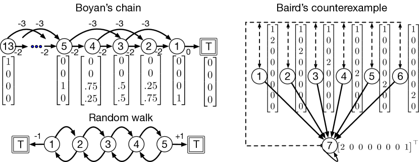
Figure 4: An illustration of the three classic RL MDPs used in our experiments, reproduced from Ghiassian et al. (2020). The illustrations of Boyan’s chain and Baird’s star counterexample include a depiction of their respective feature representations. The three feature representations used in the random walk experiments are described Section F.1.1

We first evaluate performance on a number of classic RL problems. We consider three domains, each depicted in Figure 4: a 5-state random walk with a number of different feature representations (Sutton et al., 2009), Boyan’s chain (Boyan, 2002), and Baird’s counterexample (Baird, 1995). In each of these simple problems, the RMSPBE can be computed exactly using Equation 2, and is measured after each step of interaction with the environment.

In all experiments in this section, learning curves are averaged over 200 independent runs. We tuned the step-size of the baselines over the geometric range $\alpha\in\left\{2^{-10},\ldots,2^{0}\right\}$, and step-sizes were chosen to minimize the area under the RMSPBE curve. For the CDF plots, each algorithm was given a budget of $5,000$ runs, and on each run a step-size was sampled uniformly between $2^{-1}$ and $2^{-10}$, as described in Section 4. The final RMSPBE was measured at the end of each run, and the data was aggregated as described in Section 4 to create the CDF plots. The procedure was additionally repeated with hyperparameters sampled uniformly from a discrete grid of values; the results were qualitatively similar so we omit them for brevity.

Random Walk. The random walk problem is a simple episodic undiscounted MDP, consisting of a chain of five states with terminal states on the left and right ends of the chain. The rewards are zero everywhere except when transitioning to the left or right terminal states, in which the reward is $-1$ and $+1$ respectively. Each episode begins in the middle state, and the agent follows a behavior policy which transitions left and right with equal probability. The objective is to estimate the value function of a target policy which transitions left/right with $40\%$/$60\%$ probability respectively. Following Sutton et al. (2009) and Ghiassian et al. (2020), we test three different feature representations: tabular, dependent, and inverted features. The tabular features are given by a one-hot encoding of the states (i.e. $\phi(s_{1})=(1,0,0,0,0)^{\top}$). The inverted features are the opposite encoding scheme, a “one-cold” encoding in which $[\phi(s_{i})]_{j}=1-\delta_{ij}$ for $\delta_{ij}$ being the dirac delta function. Finally, the dependent feature representation uses features $\phi(s_{1})=(1,0,0)^{\top}$, $\phi(s_{2})=(\frac{1}{\sqrt{2}},\frac{1}{\sqrt{2}},0)^{\top}$, $\phi(s_{3})=(\frac{1}{\sqrt{3}},\frac{1}{\sqrt{3}},\frac{1}{\sqrt{3}})^{\top}$, $\phi(s_{2})=(0,\frac{1}{\sqrt{2}},\frac{1}{\sqrt{2}})^{\top}$, and $\phi(s_{5})=(0,0,1)^{\top}$. Performance was measured over $3,000$ steps of interaction with the environment. Value estimates of all algorithms were initialized $\hat{v}^{\pi}(s)=0,\ \forall s\in\mathcal{S}$.

Boyan’s Chain. Boyan’s chain is a classic on-policy, episodic, undiscounted MDP. Each episode starts in the left-most state, and in state $s_{i}$ the agent transitions with equal probability to either to state $s_{i+1}$ with reward $-2$ or to state $s_{t+2}$ with reward $-3$. The exception to this rule is state $s_{1}$, in which the agent transitions deterministically to an absorbsing state with reward of $0$. This problem is frequently used to investigate the ability of an algorithm to handle representations with harmful aliasing properties — the structure of the feature representation leads to inappropriate generalization between the value estimates of adjacent states. Performance was measured over $10,000$ interactions with the environment, and the value estimates of each all algorithms were initialized to $\hat{v}^{\pi}(s)=0,\ \forall s\in\mathcal{S}$.

Baird’s Counterexample. Baird’s “star” counterexample is a well-known MDP which causes off-policy TD with linear function approximation to diverge for any scalar non-zero step-size (Baird, 1995). The MDP consists of $7$ states and two actions. The first action leads deterministically to state $7$, while the second action leads to one of the first $6$ states with equal probability. A reward of zero is received on all transitions, so the value function under any policy is $v^{\pi}(s)=0,\ \forall s\in\mathcal{S}$. The task is to estimate the value function with discount factor $\gamma=0.99$ under a deterministic target policy which chooses $\pi(s)=1$ for all states (i.e. policy which always chooses to go to state $7$), while following an equiprobable random behavior policy. The features are linearly independent and can perfectly realize the value funtion.

Performance was measured over $5,000$ steps of interaction with the environment. Value function estimates were initialized with parameters $\theta_{1}=(1,1,1,1,1,1,1,10)^{\top}$, which is the standard initialization for this problem. Note that there is no clear way make such an initialization for our coin-betting based algorithms. Typically coin-betting algorithms bet $\theta_{1}=\beta_{1}W_{0}$ with $\beta_{1}=0$ before having observed any feedback, but this is would lead to a trivial solution in Baird’s counterexample. For the CW-PF component, we choose instead $\beta_{1i}=\frac{1}{2}$ and $W_{1i}=2\theta_{1,i}$ to get $\beta_{1i}W_{0i}=\theta_{1,i}$, and similarly, for the PF component we initialize $\beta_{1}=\frac{1}{2}$, $W_{0}=2\|\theta_{1}\|$, and $u_{1}=\theta_{1}/\|\theta_{1}\|$ to give $v_{1}u_{1}=(\beta_{1}W_{0})u_{1}=\theta_{1}$.

F.1.2 Large-scale Prediction

Our final experiment tests the ability of our algorithms to scale to real-world prediction problems. The task contains many of the difficulties associated with real-world problems: the data is generated from the raw sensor readings of a mobile robot as it interacts with its environment; the data is high-dimensional, noisy, contains unpredictable changes and non-stationarities, and the prediction magnitudes can be extremely large — some reaching values in the millions — posing difficulties to learning stability.

We recreate the robot prediction task of (Modayil et al., 2014), in which the learner predicts the future sensor readings of a real mobile robot as it interacts with its environment according to a fixed behavior policy. The data was generated from each of the robot’s 53 sensors, recorded at a time interval of 100 milliseconds for a total of $120,000$ time-steps, corresponding to approximately $3$ hours of runtime of the mobile robot. The predictions in this task are formulated as $\gamma$-discounted returns with $\gamma=0.9875$, corresponding to an approximate horizon of $80$ time-steps into the future. The objective is to accurately predict these discounted returns for each of the robot’s $53$ sensors. We used the same sparse representation used in the original work, consisting of a coarse-coding of 6065 binary features. A complete description of how these features are constructed from the raw sensor readings can be found in Modayil et al. (2014). In short, a number of mappings are defined by considering a subset of the sensors and defining a discretization over the joint space of their readings; a binary feature is set depending on which cell of the grid the joint sensor reading falls into at time $t$. In particular, 457 of these mappings are defined in this experiment, leading to 457 active binary features on each time step.

For each algorithm we processed the dataset incrementally, constructing the feature vectors from the raw sensor readings and making a prediction for each sensor. At the end of the experiment, the returns $G_{t}^{(s)}$ were computed for each sensor $s$, and performance was measured in terms of the Symmetric Mean Absolute Percentage Error (SMAPE), defined by

$$\text{SMAPE}(t,s)\overset{\text{def}}{=}\frac{1}{T}\sum_{\tau=1}^{t}\frac{|\hat{v}^{(s)}(S_{\tau})-G_{\tau}^{(s)}|}{|G_{\tau}^{(s)}|+|\hat{v}^{(s)}(S_{\tau})|}.$$

The SMAPE is a relative error, and has the advantage of always being in the range $[0,1]$, making it possible to compare and aggregate the performance across different sensors. Overall performance is measured by aggregating the resulting learning curves via the median. The median is generally a better measure of aggregate performance than the mean in this problem, due to the presence of a small number of high-magnitude noisy sensors (Jacobsen et al., 2019; Modayil et al., 2014).

In this problem, we tuned the step-size of the baseline algorithms over the range $\alpha\in\left\{\frac{1}{1.785}2^{-i}:i=-16,\ldots,-2\right\}$. The range was chosen to span a wide range of possible step-sizes — from $8.5\mathrm{e}{-6}$ to $0.14$ — while also maintaining a moderate tuning budget. Step-sizes were then chosen to minimize the area under the median SMAPE curve, corresponding to the step-size which generally performs best across all sensors. Value estimates were initialized $\hat{v}^{(s)}(\cdot)=0$ for all sensors $s$.

F.2 Additional Experimental Results

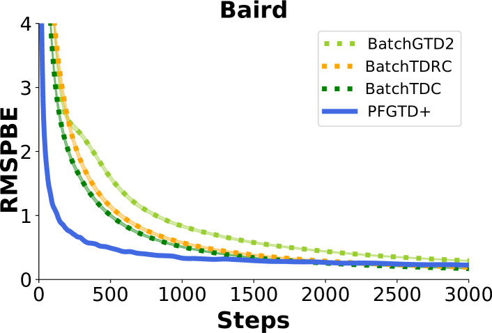
Figure 5: Performance in Baird’s counterexample when using iterate averaging. Learning curves show the accuracy of $\hat{v}^{\pi}_{t}(s)=\langle\phi(s),\overline{\theta}_{t}\rangle$, where $\overline{\theta}_{t}=\frac{1}{t}\sum_{\tau=1}^{t}\hat{\theta}_{\tau}$. Results are averaged over 200 runs, and $\pm 1$ standard error is depicted with shading.

In this section we include additional experimental results and discussion. All plots are best viewed in color.

Figure 8 (included on the last page) shows the results on the classic RL problems, with all baselines included. The plots reinforce the result of Proposition 3 as well as the conclusion made from the in-line barplot of Section 4: in all problems, PFGTD+ performs similarly to either PFGTD or CW-PFGTD — whichever happens to perform better in a given problem. Another result which seems to stand out is Baird’s counterexample, being the only problem in which the parameter-free methods fail to reach the same final performance as the baselines. Interestingly, this seems to represent a weakness of iterate averaging rather than some underlying weakness of parameter-free OLO methods. In particular, one of the key difficulties in Baird’s counterexample is that $\hat{v}(7)$ is initialized to a high value and there is only a $1/7$ change in making a transition that results in lowering $\hat{v}(7)$ towards the correct value of zero. Because of this, methods using iterate averaging end up converging to zero MSPBE only asymptotically. This can be seen in Figure 5, which shows the performance of all baselines when iterate averaging is used. We observe that when using iterate averaging, all baselines see similarly slow convergence. We recall again that the guarantees that these baselines achieve hold only under the assumption that they’re implemented with some form of iterate averaging — in a sense, this result is a more faithful representation of the performance of the baselines on this problem.

Figure 6 shows a direct comparison of the median SMAPE over time for each of the baselines. A few trends stick out immediately. First, we observe that PFGTD performs quite poorly in comparison with all other baselines. This is unsurprising as PFGTD makes use of gradient descent with step-sizes $\eta_{t}=\sqrt{2}/2\sqrt{\sum_{\tau=1}^{t}\|\widetilde{g}_{t}\|^{2}}$ as a component in its hierarchy of reductions; the combination of high-dimensional features and high-magnitude sensor readings quickly drives the step-sizes towards zero. Yet, the features are quite sparse, so few (if any) updates get made to each of the parameters managed by this sub-procedure before the step-size is small enough to impede learning, leading to poor performance we see in these figures. Second, we observe a slight upward trend in the SMAPE of PFGTD+ after it reaches its lowest point. This illustrates another drawback associated with iterate averaging: the data is non-stationary, so converging to a fixed solution inevitably leads to some unwanted drift in performance thereafter. In practice this could likely be avoided by using an exponential moving average, for example, though this would require choosing a decay rate. Doing so without tuning hyperparameters is non-trivial and is an ongoing direction of future work. Finally, we observe that none of the gradient-based methods are able to compete with TD in this problem. Though this is the case in general, the performance gap appears to be particularly pronounced in this problem. We conjecture that this is related to non-stationarity of the data; the gradient-based algorithms are likely less able to track non-stationary data in general, due the interactions between the primary and secondary parameters $\theta_{t}$ and $y_{t}$.

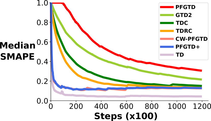
Figure 6: Median SMAPE across all sensors in the large-scale prediction task. Baseline step-sizes were tuned over the values $\alpha\in\left\{\frac{1}{1.785}2^{-i}:i=-16,\ldots,-2\right\}$, and chosen to minimize the area under the median SMAPE curve.

The unaggregated performance of each algorithm in the large-scale prediction task is depicted in Figure 7. Each plot in the grid shows a given algorithm’s performance on each of the individual sensors, with the median performance shown in black. The plot for PFGTD+ is repeated in each row to enable easy comparison to the baselines. The plots show that PFGTD+ achieves favorable performance over TDC and TDRC not only in the median, but in general across sensors in this problem. The second row of plots demonstrates that PFGTD+ performs nearly identically to CW-PFGTD, despite the fact that it also uses iterates from the PF subroutine which performs poorly in this specific problem, further demonstrating Proposition 3.

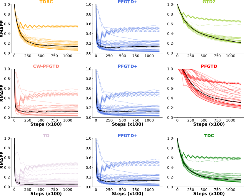
Figure 7: SMAPE over time for each individual sensor in the large-scale prediction task. Each colored line represents the SMAPE between the learner’s predictions and the true discounted sum of future sensor readings for a given sensor, with the median shown in black. The plots are arranged in a grid to facilitate direct visual comparison between the proposed algorithm, PFGTD+, and each of the baselines.

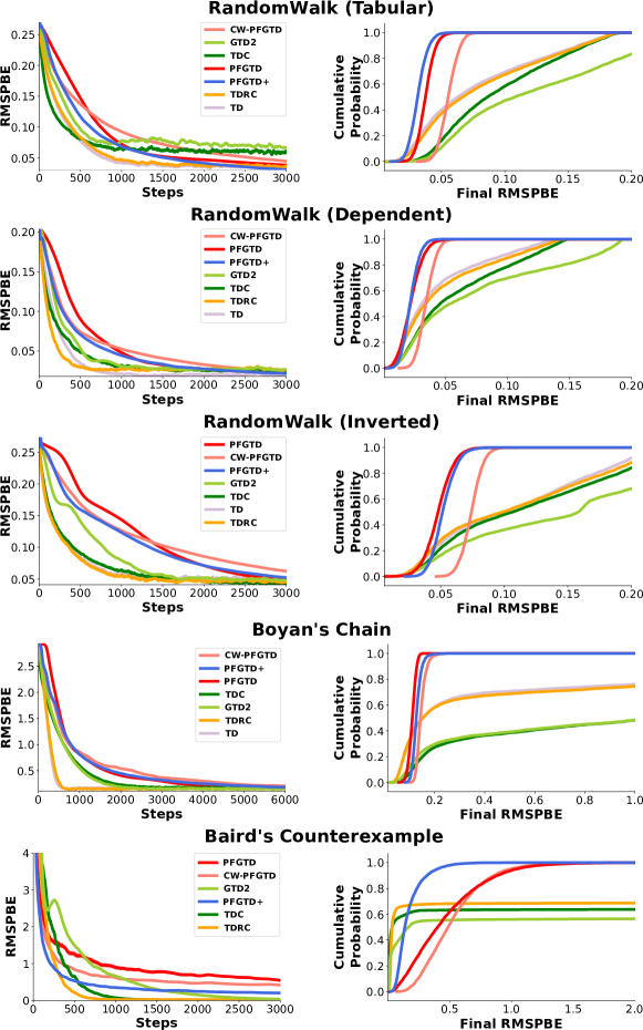
Figure 8: Learning curves and CDF plots for each of the classic RL tasks (view in color). Left column: Learning curves for each of the classic RL tasks. Results are averaged over 200 independent runs. $\pm 1$ standard error is shaded around each of the lines, but it is generally vanishingly small. Baseline hyperparameters were tuned over the range $\alpha\in\left\{2^{-i}:i=0,\ldots,10\right\}$, and were chosen to minimize the area under the learning curve. Right column: CDF plots for each of the classic RL tasks. Each plot depicts the distribution of final RMSPBE over a sample of 5,000 independent runs. Hyperparameters of baseline algorithms were sampled uniformly between $[2^{0},2^{-10}]$. The experiment was also repeated with hyperparameters sampled from a discrete grid of values; the results were qualitatively similar and have been omitted for brevity.

References

- Baird (1995) Baird, L. Residual algorithms: Reinforcement learning with function approximation. In Machine Learning Proceedings 1995, pp. 30–37. Elsevier, 1995.
- Bhaskara et al. (2020) Bhaskara, A., Cutkosky, A., Kumar, R., and Purohit, M. Online linear optimization with many hints. In Advances in Neural Information Processing Systems, 2020.
- Boyan (2002) Boyan, J. A. Technical update: Least-squares temporal difference learning. Machine learning, 49(2-3):233–246, 2002.
- Boyd & Vandenberghe (2004) Boyd, S. and Vandenberghe, L. Convex optimization. Cambridge university press, 2004.
- Cesa-Bianchi et al. (2004) Cesa-Bianchi, N., Conconi, A., and Gentile, C. On the generalization ability of on-line learning algorithms. IEEE Transactions on Information Theory, 2004.
- Cutkosky (2019a) Cutkosky, A. Artificial constraints and hints for unbounded online learning. In Conference on Learning Theory, pp. 874–894, 2019a.
- Cutkosky (2019b) Cutkosky, A. Combining online learning guarantees. arXiv preprint arXiv:1902.09003, 2019b.
- Cutkosky (2020) Cutkosky, A. Parameter-free, dynamic, and strongly-adaptive online learning. In International Conference on Machine Learning, volume 2, 2020.
- Cutkosky & Orabona (2018) Cutkosky, A. and Orabona, F. Black-box reductions for parameter-free online learning in banach spaces. arXiv preprint arXiv:1802.06293, 2018.
- Ghadimi & Lan (2013) Ghadimi, S. and Lan, G. Stochastic first-and zeroth-order methods for nonconvex stochastic programming. SIAM Journal on Optimization, 23(4):2341–2368, 2013.
- Ghiassian et al. (2020) Ghiassian, S., Patterson, A., Garg, S., Gupta, D., White, A., and White, M. Gradient Temporal-Difference Learning with Regularized Corrections. In Proceedings of the 37 th International Conference on Machine Learning, volume 119, Vienna, Austria, 2020. PMLR.
- Grimm et al. (2020) Grimm, C., Barreto, A., Singh, S., and Silver, D. The value equivalence principle for model-based reinforcement learning. arXiv preprint arXiv:2011.03506, 2020.
- Hazan et al. (2007) Hazan, E., Agarwal, A., and Kale, S. Logarithmic regret algorithms for online convex optimization. Machine Learning, 2007.
- Henderson et al. (2018) Henderson, P., Romoff, J., and Pineau, J. Where did my optimum go?: An empirical analysis of gradient descent optimization in policy gradient methods. CoRR, abs/1810.02525, 2018. URL http://arxiv.org/abs/1810.02525.
- Henderson et al. (2019) Henderson, P., Islam, R., Bachman, P., Pineau, J., Precup, D., and Meger, D. Deep reinforcement learning that matters, 2019.
- Jacobsen et al. (2019) Jacobsen, A., Schlegel, M., Linke, C., Degris, T., White, A., and White, M. Meta-descent for online, continual prediction. In AAAI Conference on Artificial Intelligence, 2019.
- Juditsky et al. (2019) Juditsky, A., Nazin, A., Nemirovsky, A., and Tsybakov, A. Algorithms of robust stochastic optimization based on mirror descent method. arXiv preprint arXiv:1907.02707, 2019.
- Jun & Orabona (2019) Jun, K.-S. and Orabona, F. Parameter-free online convex optimization with sub-exponential noise. In Proceedings of the Thirty-Second Conference on Learning Theory, 2019.
- Kearney et al. (2018) Kearney, A., Veeriah, V., Travnik, J. B., Sutton, R. S., and Pilarski, P. M. Tidbd: Adapting temporal-difference step-sizes through stochastic meta-descent. arXiv:1804.03334, 2018.
- Kingma & Ba (2014) Kingma, D. P. and Ba, J. Adam: A method for stochastic optimization. arXiv preprint arXiv:1412.6980, 2014.
- Liu et al. (2018) Liu, B., Gemp, I., Ghavamzadeh, M., Liu, J., Mahadevan, S., and Petrik, M. Proximal gradient temporal difference learning: Stable reinforcement learning with polynomial sample complexity. Journal of Artificial Intelligence Research, 2018.
- Liu et al. (2019) Liu, V., Kumaraswamy, R., Le, L., and White, M. The utility of sparse representations for control in reinforcement learning. In Proceedings of the AAAI Conference on Artificial Intelligence, 2019.
- McMahan & Orabona (2014) McMahan, H. B. and Orabona, F. Unconstrained online linear learning in hilbert spaces: Minimax algorithms and normal approximations. 2014.
- Mertikopoulos et al. (2018) Mertikopoulos, P., Lecouat, B., Zenati, H., Foo, C.-S., Chandrasekhar, V., and Piliouras, G. Optimistic mirror descent in saddle-point problems: Going the extra (gradient) mile. arXiv preprint arXiv:1807.02629, 2018.
- Mhammedi & Koolen (2020) Mhammedi, Z. and Koolen, W. M. Lipschitz and comparator-norm adaptivity in online learning. In Conference on Learning Theory, 2020.
- Mhammedi et al. (2019) Mhammedi, Z., Koolen, W. M., and Van Erven, T. Lipschitz adaptivity with multiple learning rates in online learning. In Conference on Learning Theory, 2019.
- Modayil et al. (2014) Modayil, J., White, A., and Sutton, R. S. Multi-timescale nexting in a reinforcement learning robot. Adaptive Behavior, 22(2):146–160, 2014.
- Nemirovski et al. (2009) Nemirovski, A., Juditsky, A., Lan, G., and Shapiro, A. Robust stochastic approximation approach to stochastic programming. SIAM Journal on optimization, 2009.
- Orabona (2019) Orabona, F. A modern introduction to online learning, 2019.
- Orabona & Pál (2016) Orabona, F. and Pál, D. Coin betting and parameter-free online learning. Advances in Neural Information Processing Systems, 2016.
- Orabona & Pál (2018) Orabona, F. and Pál, D. Scale-free online learning. Theoretical Computer Science, 2018.
- Schlegel et al. (2021) Schlegel, M., Jacobsen, A., Abbas, Z., Patterson, A., White, A., and White, M. General value function networks. Journal of Artificial Intelligence Research, 70, 2021.
- Schraudolph (1999) Schraudolph, N. N. Local gain adaptation in stochastic gradient descent. International Conference on Artificial Neural Networks, 1999.
- Sutton (1988) Sutton, R. S. Learning to predict by the methods of temporal differences. Machine learning, 3(1):9–44, 1988.
- Sutton et al. (2009) Sutton, R. S., Maei, H. R., Precup, D., Bhatnagar, S., Silver, D., Szepesvári, C., and Wiewiora, E. Fast gradient-descent methods for temporal-difference learning with linear function approximation. In Proceedings of the 26th Annual International Conference on Machine Learning, 2009.
- Veeriah et al. (2019) Veeriah, V., Hessel, M., Xu, Z., Rajendran, J., Lewis, R. L., Oh, J., van Hasselt, H. P., Silver, D., and Singh, S. Discovery of useful questions as auxiliary tasks. In Advances in Neural Information Processing Systems 32. 2019.