Approximate Fréchet Mean for Data Sets of Sparse Graphs

Abstract

To characterize the location (mean, median) of a set of graphs, one needs a notion of centrality that is adapted to metric spaces, since graph sets are not Euclidean spaces. A standard approach is to consider the Fréchet mean. In this work, we equip a set of graph with the pseudometric defined by the $\ell_{2}$ norm between the eigenvalues of their respective adjacency matrix . Unlike the edit distance, this pseudometric reveals structural changes at multiple scales, and is well adapted to studying various statistical problems on sets of graphs. We describe an algorithm to compute an approximation to the Fréchet mean of a set of undirected unweighted graphs with a fixed size.

1 Introduction

Machine learning from a set of data almost always requires some notion of average. Algorithms for clustering, classification, and linear regression all utilize the average value of the data set [17]. When the distance is induced by a norm, then the mean is a simple algebraic operation. If the data lie on a Riemannian manifold, equipped with a metric, then one can extend the notion of mean with the concept of Fréchet mean [28]. In fact the concept of Fréchet mean only requires that a (pseudo)metric between points be defined, and therefore one can consider the Fréchet mean of a set in a pseudometric space [13]. Not surprisingly, many machine learning algorithms, which were developed for Euclidean spaces, can be extended to use the Fréchet mean. The purpose of this paper is to solve the nontrivial problem of determining the Fréchet mean for data sets of graphs when the pseudometric is the $\ell_{2}$ distance between the eigenvalues of the adjacency matrix.

In this work we consider a set of simple graphs with $n$ vertices. The graphs are considered to be sparse, in the sense that the edge density satisfies,

$$\rho_{n}=\Omega\left(\frac{\ln^{3}(n)}{n}\right).$$ (1)

Because most real world networks are sparse, this constraint is realistic. We additionally note that the vertex set must be sufficiently large and that the technique introduced in this paper will perform poorly for sets of small graphs.

Our line of attack involves the following two intermediate results: (1) the Fréchet mean of a set of sparse graphs can be approximated within any precision by a stochastic block model; (2) given a sequence of eigenvalues of an adjacency matrix, one can recover the stochastic block model whose spectrum matches these target eigenvalues. We prove various error bounds and convergence results for our algorithm and validate the theory with several experiments. The paper is structured as follows: section 3 introduces the notations used to refer to graphs and sets of graphs as well as defining precisely what is meant by a random graph and a stochastic block model ensemble. Section 4 defines the Fréchet mean problem, its empirical alternative, and introduces the theorems necessary for our solution. Section 7 describes briefly how the Fréchet mean applies to regression for graph valued data sets and section 6 introduces a numerical method to find the Fréchet mean. Section 8 serves to experimentally validate the theory of the previous sections. We leave all proofs of our results to the appendix.

2 State of the Art

We consider a set of undirected unweighted graphs of fixed size $n$, $\mathcal{G}$, wherein we define a distance . To characterize the location (mean, median) of the set $\mathcal{G}$, we need a notion of centrality that is adapted to metric spaces, since graph sets are not Euclidean spaces. A standard approach is to consider the Fréchet sample mean, and the Fréchet total sample variance.

The choice of metric is crucial to the computation of the Fréchet mean, since each metric induces a different mean graph. The Fréchet mean of graphs has been studied in the context where the distance is the edit distance (e.g., [7, 15, 19, 18, 22] and references therein). The edit distance reflects small scale changes in the graphs and therefore the Fréchet mean will be sensitive to the fine structural distinctions between graphs. Effectively, the Fréchet mean with respect to the edit distance can then be interpreted as an average of the fine structures in the observed graphs as measured by this distance.

In this paper, we consider that the fine scale, which is defined by the local connectivity at the level of each vertex, may be intrinsically random. The quantification of such random fluctuations is uninformative when comparing graphs. We prefer to use a distance that can detect larger scale patterns of connectivity that happen at multiple scales.

The adjacency spectral distance, which is just the $\ell_{2}$ norm of the difference between the spectra of the adjacency matrices of the two graphs of interest [36], exhibits good performance when comparing various types of graphs [35], making it a reliable choice for a wide range of problems. Spectral distances also exhibit practical advantages, as they can inherently compare graphs of different sizes and can compare graphs without known vertex correspondence (see e.g., [11, 10] and references therein). The adjacency spectrum in particular is well-understood, and is perhaps the most frequently studied graph spectrum [9, 12].

In practice, it is often the case that only the first $c$ eigenvalues are compared, where $c\ll n$. We still refer to such truncated spectral distances as spectral distances. Comparison using the first $c$ eigenvalues for small $c$ allows one to focus on the community structure of the graph, while ignoring the local structure of the graph [24]. Inclusion of the highest-$c$ eigenvalues allows one to discern local features as well as global. This flexibility allows the user to target the particular scale at which she wishes to study the graph, and is a significant advantage of the spectral distances.

Instead of solving the minimization problem associated with the computation of the Fréchet mean in the original set $\mathcal{G}$, the authors in [11] suggest to embed the graphs in Euclidean space, wherein they can trivially find the mean of the set. Because the embedding in [11] is not an isometry, there is no guarantee that the inverse of the average embedded graphs be equal to the Fréchet mean. Furthermore, the inverse embedding may not be available in closed form. In the case of simple graphs, the Laplacian matrix of the graph uniquely characterizes the graph. The authors in [16] define the mean of a set of graphs using the Fréchet sample mean (computed on the manifold defined by the cone of symmetric positive semi-definite matrices) of the respective Laplacian matrices.

3 Notation

We denote by $G=(V,E)$ a graph with vertex set $V=\{1,2,...,n\}$ and edge set $E\subset V\times V$. For vertices $i,j\in V$ an edge exists between them if the pair $(i,j)\in E$. The size of a graph is called $n=|V|$ and the number of edges is $m=|E|$. The density of a graph is called $\rho_{n}=\frac{m}{n(n-1)/2}$. For any $n>100$, we say a graph is sparse when

$$\rho_{n}=\Omega\left(\frac{\ln^{3}(n)}{n}\right).$$ (2)

The matrix $\bm{A}$ is the adjacency matrix of the graph and is defined as

$$\bm{A}_{ij}=\begin{cases}1\quad\text{if }(i,j)\in E,\\ 0\quad\text{else.}\end{cases}$$

We define the function $\sigma$ to be the mapping from the set of $n\times n$ adjacency matrices (square, symmetric matrices with zero entries on the diagonal), $\operatorname{\mathbb{M}}_{n\times n}$ to $\operatorname{\mathbb{R}}^{n}$ that assigns to an adjacency matrix the vector of its $n$ sorted eigenvalues,

$$\sigma:\operatorname{\mathbb{M}}_{n\times n} \longrightarrow\operatorname{\mathbb{R}}^{n},$$ (3)

$$\bm{A} \longmapsto\bm{\lambda}=[\lambda_{1},\ldots,\lambda_{n}],$$ (4)

where $\lambda_{1}\geq\ldots\geq\lambda_{n}$ Because we often consider the $c$ largest eigenvalue of the adjacency matrix $\bm{A}$, we define the mapping to the truncated spectrum as $\sigma_{c}$ ,

$$\sigma_{c}:\operatorname{\mathbb{M}}_{n\times n} \longrightarrow\operatorname{\mathbb{R}}^{c},$$ (5)

$$\bm{A} \longmapsto\bm{\lambda}_{c}=[\lambda_{1},\ldots,\lambda_{c}].$$ (6)

We write $G\tilde{=}G^{\prime}$ when two graphs are isomorphic. Two graphs are isomorphic if and only if there exists a permutation matrix $\bm{P}$ such that $\bm{A}^{\prime}=\bm{P}^{T}\bm{A}\bm{P}$.

Definition 1 (Adjacency spectral pseudometric)

We define the adjacency spectral pseudometric as the $\ell_{2}$ norm between the spectra of the respective adjacency matrices,

$$d_{A}(G,G^{\prime})=||\sigma(G)-\sigma(G^{\prime})||_{2}.$$ (7)

The pseudometric $d_{A}$ satisfies the symmetry and triangle inequality axioms, but not the identity axiom. Instead, $d_{A}$ satisfies the reflexivity axiom

$$d_{A}(G,G)=0,\quad\forall G\in\mathcal{G}.$$

We define the truncated adjacency spectral pseudometric as

$$d_{A_{c}}(G,G^{\prime})=||\sigma_{c}(G)-\sigma_{c}(G^{\prime})||_{2}.$$ (8)

Definition 2 (Set of graphs and sparse graphs)

We denote by $\mathcal{G}$ the set of all simple graphs on $n$ nodes.

Furthermore, we denote by $\mathcal{G}_{s}\subset\mathcal{G}$ the subset of sparse graphs for which the edge density satisfies

$$\rho(G)=\frac{2m}{n(n-1)}=\Omega\left(\frac{\ln^{3}(n)}{n}\right)$$ (9)

where $m$ is the number of edges of $G$.

3.1 Random Graphs

We denote by $\operatorname{\mathcal{M}}(\mathcal{G})$ the space of probability measures on $\mathcal{G}$. In this work, when we talk about a measure we always mean a probability measure.

Definition 3 (Set of random graphs associated with a measure $\mu$)

Let $\mathcal{H}$ be a subset of $\mathcal{G}$, and $\mu$ a probability measure defined on $\mathcal{H}$. We can extend $\mu$ to $\mathcal{G}$, such that for any $\mathcal{A}\subset\mathcal{G}$, we define $\mu(\mathcal{A})=\mu(\mathcal{A}\cap\mathcal{H})$. We define the set of random graphs distributed according to $\mu$ to be the probability space $\left(\mathcal{H},\mu\right)$.

Remark 1

In this paper, the $\sigma$-field associated with the $\left(\mathcal{H},\mu\right)$ will always be the power set of $\mathcal{H}$.

This definition allows to recast various ensemble of random graphs (e.g., Erdős-Rényi, inhomogeneous Erdős-Rényi, stochastic block models, etc) using a unique notation.

3.1.1 Kernel Probability Measures

Let $\left\{\xi_{i}\right\}_{i=1}^{n}$ be the sequence of equispaced points in the interval $[0,1]$, $\xi_{i}=i/n$.

Definition 4 (kernel probability measure)

A probability measure $\mu\in\operatorname{\mathcal{M}}(\mathcal{G})$ is called a kernel probability measure if there exist a subset $\mathcal{H}\subset\mathcal{G}$ and a function $f$,

$$f:[0,1]\times[0,1]\mapsto(0,1),$$ (10)

such that $f(x,y)=f(1-y,1-x)$, and such that

$$\forall G\in\mathcal{H},\text{with adjacency matrix}\;\bm{A}=\left(a_{ij}\right),\mu\left(\left\{\bm{A}\right\}\right)=\mspace{-12.0mu}\prod_{1\leq i<j\leq n}\mspace{-12.0mu}\mathbb{P}\left(a_{ij}\right)=\mspace{-12.0mu}\prod_{1\leq i<j\leq n}\mspace{-12.0mu}\operatorname{Bernoulli}\left(f(\xi_{i},\xi_{j})\right).$$ (11)

The function $f$ is called a kernel of $\mu$.

Definition 5

We denote by $\mathcal{K}$ the set of all kernel functions,

$$\mathcal{K}=\left\{f|f:[0,1]^{2}\mapsto(0,1);f(x,y)=f(1-y,1-x)\right\}.$$ (12)

We note that given the sequence $\left\{\xi_{i}\right\}\;1\leq i\leq n$ and the measure $\mu$, the kernel $f$ forms an equivalence class of functions, characterized by their values on the grid $\left\{(\xi_{i},\xi_{i})\;1\leq i,j\leq n\right\}$.

Remark 2

Many definitions of random graphs allow for $\{\xi_{i}\}$ to be a random sample from some probability density function on $[0,1]$ (e.g., [5, 23, 21, 26], and references therein) With the right distribution defined on $[0,1]$, many of the results would be identical when taking an expectation over the random sample $\{\xi_{i}\}$. The advantage to specifying the points as an equispaced grid allows a greater level of control when specifying certain properties of the kernels. For example, we will be able to guarantee the number of nodes in a community when considering kernels of stochastic block models, which we define in the following section.

Notation 1

We denote by $G_{\mu}$ a random realization of a graph $G\in\left(\mathcal{G},\mu\right)$. Sometimes, we use the notation $G(n,f)$ if $\mu$ is kernel probability measure. This notation generalizes the notation of the classic Erdős-Rényi random graphs of $G(n,p)$ where taking $f(x,y)=p$ is a possible kernel as in [20].

Notation 2

Given a measurable function $\varphi$ defined on the probability space $\left(\mathcal{G},\mu\right)$, we denote by $\mathbb{E}_{\mu}\mspace{-4.0mu}\left[\varphi\right]$ the expected value $\mathbb{E}\left[\varphi(G)\right]$, when $G$ is distributed according to $\mu$.

Definition 6

Given a kernel probability measure $\mu$ with kernel $f$ we denote by

$$\mathbb{E}_{\mu}\mspace{-4.0mu}\left[\rho_{n}\right]=\frac{\sum_{i>j}f(\xi_{i},\xi_{j})}{n(n-1)/2},$$ (13)

the expected density of the measure $\mu$ on the grid $\left\{(\xi_{i},\xi_{i})\;1\leq i,j\leq n\right\}$.

3.1.2 Stochastic Block Models

The stochastic block model [1] plays an important role in this work. We review the specific features of this model using the notations that were defined in the previous paragraphs. The key aspects of the model are: the geometry of the blocks, the within-community edges densities, and the across-community edge density.

We assume that there exists a large constant $C$ that provides an upper bound on the number of communities; the actual number of non empty communities is denoted by $c\leq C$.

The geometry of the stochastic block model is encoded using the relative sizes of the communities. We denote by $\bm{s}\in[0,1]^{c}$ the vector of relative sizes of each of the $c$ blocks. We have $0<s_{k}\leq 1$, and $\sum_{k=1}^{c}s_{k}=1.$

The edge density within a non empty block $k$, is denoted by $p_{k}$. We can concatenate the $p_{k}$ into a vector $\bm{p}=\begin{bmatrix}p_{1}\cdots p_{c}\end{bmatrix}$, which describes the within-block edges densities. Finally, we denote by $q$ the across-community edge density.

We can parameterize a stochastic block model using one representative of the equivalence class of kernel, $f$. We simply consider the function $f$, which is piecewise constant over the blocks, and is defined by

$$f:[0,1]\times[0,1] \longrightarrow(0,1)$$ (14)

$$(x,y) \longmapsto\begin{cases}p_{k}&\text{if}\quad\sum_{j=1}^{k-1}s_{k}\leq x<\sum_{j=1}^{k}s_{k},\;\text{and}\quad\sum_{j=1}^{k-1}s_{k}\leq y<\sum_{j=1}^{k}s_{k},\\ q&\text{otherwise.}\end{cases}$$ (15)

This piecewise constant function is called the canonical kernel associated to the block model with measure $\mu$ (see, e.g. Fig. 1), and we denote it by $f(x,y,\bm{p},q,\bm{s})$.

Example 1

Given $\bm{s}=\begin{bmatrix}1/2&1/4&1/4&0\cdots\end{bmatrix}^{T}$ the values of $f(x,y;\bm{p},q,\bm{s})$ in the unit square are shown in Fig. 1

Given the edges densities $(\bm{p},q)$, a block geometry $\bm{s}$, and a graph size $n$, we can generate a random realization of the stochastic block model with kernel $f(x,y,\bm{p},q,\bm{s})$ by sampling the entries of its adjacency matrix $\bm{A}=\left(a_{ij}\right)$ according to,

$$a_{i,j}\sim\operatorname{Bernoulli}\left(f(\xi_{i},\xi_{j};\bm{p},q,\bm{s}\right),\;a_{ji}=a_{ij},\;\text{and}\;a_{ii}=0,\quad 1\leq i<j\leq n.$$ (16)

Using the generalized Erdős-Rényi notation a random graph from the stochastic block model is denoted by

$$G(n,f(x,y;\bm{p},q,\bm{s})).$$ (17)

Definition 7

We denote by $\mathcal{K}_{{\mathop{\scriptscriptstyle\mathrm{SBM}}}}$ the set of piecewise constant functions on $[0,1]\times[0,1]$ that are canonical kernels of stochastic block models,

$$\mathcal{K}_{{\mathop{\scriptscriptstyle\mathrm{SBM}}}}=\left\{f(x,y;\bm{p},q,\bm{s});c\in\operatorname{\mathbb{N}},\bm{p}\in[0,1]^{c},q\in[0,1],\bm{s}\in[0,1]^{c},\sum_{k=1}^{c}s_{k}=1\right\}$$ (18)

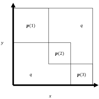
Figure 1: Example $f(x,y;\bm{p},q,\bm{s})$

Defining the ensemble in this way allows for the smooth introduction of new communities by allowing the vector $\bm{s}$ to continuously increase in size. Additionally, defining the parameters independently of the number of nodes naturally allows for large graph limits to be explored.

For a fixed $n$, and a canonical kernel $f_{{\mathop{\scriptscriptstyle\mathrm{SBM}}}}\in K_{{\mathop{\scriptscriptstyle\mathrm{SBM}}}}$, there exists a unique induced probability measure, which we denote by $\mu_{{\mathop{\scriptscriptstyle\mathrm{SBM}}}}(\bm{p},q,\bm{s},n)$.

Definition 8

The set of all probability measures induced by the set $K_{{\mathop{\scriptscriptstyle\mathrm{SBM}}}}$ is denoted by

$$\operatorname{\mathcal{M}}_{{\mathop{\scriptscriptstyle\mathrm{SBM}}}}(\mathcal{G})=\{\mu_{{\mathop{\scriptscriptstyle\mathrm{SBM}}}}|\mu_{{\mathop{\scriptscriptstyle\mathrm{SBM}}}}\text{ is induced by }f_{{\mathop{\scriptscriptstyle\mathrm{SBM}}}}\in K_{{\mathop{\scriptscriptstyle\mathrm{SBM}}}}\}.$$ (19)

Sometimes we suppress the parameters and write $\mu_{{\mathop{\scriptscriptstyle\mathrm{SBM}}}}\in\operatorname{\mathcal{M}}_{{\mathop{\scriptscriptstyle\mathrm{SBM}}}}(\mathcal{G})$.

4 The Fréchet mean and Empirical Fréchet Mean

We consider $\mathcal{G}$ the space of graphs defined on sets of $n$ vertices. We equip that space with the pseudometric defined by the $\ell_{2}$ norm between the spectra of the respective adjacency matrices, $d_{A}$, (see (7)). We consider a probability measure in $\mu\in\operatorname{\mathcal{M}}$ that describes the chances of obtaining a given graph when we sample $\mathcal{G}$ according to $\mu$. Using $d_{A}$, we can quantify the spread of the graphs, and we can also define a notion of centrality, which gives the location of the average graph, according to $\mu$.

Definition 9 (Fréchet mean [13])

The Fréchet mean of the pseudometric space $(\mathcal{G},d)$, where $d$ is the pseudometric (7), equipped with probability measure $\mu$ is the set of graphs $G^{*}$ whose expected distance to $\mathcal{G}$ is minimum,

$$\left\{G^{*}\in\mathcal{G}\right\}=\underset{G\in\mathcal{G}}{\operatorname{argmin}}\mspace{4.0mu}\mathbb{E}_{\mu}\mspace{-4.0mu}\left[d^{2}(G,G_{\mu})\right].$$ (20)

where $G_{\mu}$ is a random realization of a graph from the probability space $\left(\mathcal{G},\mu\right)$ , and the expectation $\mathbb{E}_{\mu}\mspace{-4.0mu}\left[d^{2}(G,G_{\mu})\right]$ is computed with respect to the probability measure $\mu$.

In this work, we assume that the Fréchet mean both exists and is unique. Therefore $\mathcal{M}^{*}$ is a singleton and we write the Fréchet mean as

$$G^{*}=\underset{G\in\mathcal{G}}{\text{argmin }}\mathbb{E}_{\mu}\mspace{-4.0mu}\left[d^{2}(G,G_{\mu})\right].$$ (21)

As we change $\mu$ we expect that, for a fixed $G$, $\mathbb{E}_{\mu}\mspace{-4.0mu}\left[d^{2}(G,G_{\mu})\right]$ will change, and therefore the Fréchet mean $G^{*}$ will move inside $\mathcal{G}$ for different choices of the probability measure $\mu$. $G^{*}$ plays the role of the center of mass, for the mass distribution associated with $\mu$. We make this dependency explicit by defining the Fréchet mean map.

Definition 10 (The Fréchet mean map)

Given the set of graphs $\mathcal{G}$, the Fréchet mean map assigns to a probability measure $\mu\in\operatorname{\mathcal{M}}(\mathcal{G})$ the corresponding Fréchet mean,

$$\mathop{\mathfrak{F}}(\mu)=\underset{G\in\mathcal{G}}{\operatorname{argmin}}\mspace{4.0mu}\mathbb{E}_{\mu}\mspace{-4.0mu}\left[d^{2}(G,G_{\mu})\right].$$ (22)

For a fixed $\mu$ we may write the Fréchet mean as $G^{*}=\mathop{\mathfrak{F}}(\mu).$ The Fréchet mean map is of significant importance throughout this paper and the map $\mathop{\mathfrak{F}}$ will be referred to throughout many theorems, equations, and proofs.

In practice, the only information known about a distribution on $\mathcal{G}$ comes from a sample of graphs. Therefore, we need a notion of Fréchet sample mean, which is defined as follows.

Definition 11 (Empirical Fréchet mean)

Let $\mu$ be a probability measure on $\mathcal{G}$, and let $\left\{G_{i}\right\}\;1\leq i\leq N$ be a random sample from the probability space $\left(\mathcal{G},\mu\right)$. The empirical Fréchet mean is defined by

$$G_{N}^{*}=\underset{G\in\mathcal{G}}{\operatorname{argmin}}\mspace{4.0mu}\sum_{i=1}^{N}d^{2}(G,G_{i}).$$ (23)

We additionally assume that the empirical Fréchet mean exists and is unique for any given sample of graphs. The dependence on $N$ is explicitly given but may be suppressed throughout the paper when it is obvious.

Remark 3

Because the pseudometric $d$ (see (7)) in (23) is the $\ell^{2}$ distance between the spectra of $G$ and $G_{i}$ respectively, $G_{N}^{*}$ is the unique minimizer for (23) if and only if

$$\sigma(G_{N}^{*})=\frac{1}{N}\sum_{i=1}^{N}\sigma(G_{i}).$$ (24)

There exists several computational algorithms to solve the inverse eigenvalue problem,

$$G^{*}_{N}=\sigma^{-1}\left(\frac{1}{N}\sum_{i=1}^{N}\sigma(G_{i})\right).$$ (25)

Some recent work in this field is presented in [4, 30]. The work in [4] involves knowledge of a graph’s adjacency matrix to generate different graphs with similar spectra. The work in [30] is very closely related to the ideas presented in this paper, however they utilize the spectra of the normalized Laplacian matrix and construct adjacency matrices that will have similar spectra. This work is exciting but the algorithms presented are not currently fully supported with theory.

Instead, we propose to solve the inverse eigenvalue problem over the space of sparse SBM graph models. Specifically, we construct an SBM model, whose Freéchet mean is $\varepsilon$ away from $G^{*}_{N}$, according to the truncated spectral pseudometric,

$$d_{A_{c}}(G_{N}^{*},G_{{\mathop{\scriptscriptstyle\mathrm{SBM}}}}^{*})<\varepsilon.$$ (26)

5 Main Results

We are now in position to state the main results of the paper. The next theorem constitutes the main theorem.

Theorem 1 (An approximation to the empirical Fréchet mean with respect to $d_{A_{c}}$)

Let $\mu\in\operatorname{\mathcal{M}}\left(\mathcal{G}\right)$, and let $\left\{G_{i}\right\}\;1\leq i\leq N$ be a random sample of sparse graphs sampled from the probability space $\left(\mathcal{G}_{s},\mu\right)$. Let

$$G_{N}^{*}=\underset{G\in\mathcal{G}}{\operatorname{argmin}}\mspace{4.0mu}\sum_{i=1}^{N}d_{A_{c}}^{2}(G,G_{i})$$ (27)

be the empirical Fréchet mean of the sample $\left\{G_{i}\right\}\;1\leq i\leq N$. Then, as the size $n$ of the graphs in $\mathcal{G}$ goes to infinity,

$$\forall\varepsilon>0,\;\exists\mu_{{\mathop{\scriptscriptstyle\mathrm{SBM}}}}\in\operatorname{\mathcal{M}}_{{\mathop{\scriptscriptstyle\mathrm{SBM}}}}(\mathcal{G}),\;\text{such that}\;d_{A_{c}}(G^{*}_{N},\mathop{\mathfrak{F}}(\mu_{{\mathop{\scriptscriptstyle\mathrm{SBM}}}}))<\varepsilon.$$ (28)

Proof of Theorem 1

The proof relies on theorem 2 and conjecture 1. Let $\left\{G_{i}\right\}\;1\leq i\leq N$ be a random sample from the probability space of sparse graph $\left(\mathcal{G}_{s},\mu\right)$. As a consequence of conjecture 1, $G^{*}$, the Fréchet mean of $\left\{G_{i}\right\}\;1\leq i\leq N$ is sparse. We now apply theorem 2 to $G^{*}\in\mathcal{G}_{s}$,

$$\forall\varepsilon>o,\;\exists\mu_{{\mathop{\scriptscriptstyle\mathrm{SBM}}}}\in\operatorname{\mathcal{M}}_{{\mathop{\scriptscriptstyle\mathrm{SBM}}}}(\mathcal{G}),\;\text{such that}\;d_{A_{c}}(G^{*},\mathop{\mathfrak{F}}(\mu_{{\mathop{\scriptscriptstyle\mathrm{SBM}}}}))<\varepsilon.$$ (29)

$\square$

The intuition for theorem 1 comes from acknowledging that there are many distributions with the same first moment. To utilize this idea, we need only to find a distribution $\nu$ whose first moment is the same as the empirical Fréchet mean given the set of observed graphs $M$.

The metric chosen in theorem 1 is specifically $d_{A_{c}}$. This metric measures the difference in the largest $c$ eigenvalues of two graphs. It is well known that the largest $c$ eigenvalues of a stochastic block model with $c$ blocks completely encodes the community structure. Since the community structure is a global property of the graph, we claim that other global structures of the graphs are captured by the largest $c$ eigenvalues. As a consequence, we claim that the global properties of the empirical Fréchet mean, $G_{N}^{*}$, are similar to the global properties of the approximate empirical Fréchet mean, $G_{{\mathop{\scriptscriptstyle\mathrm{SBM}}}}^{*}$.

Theorem 1 shows that we need only to find the parameters of the suitable stochastic block model and compute its Fréchet mean. The identification of the optimal set of parameters for the stochastic block model is a non-trivial problem. One approach to determine $(\bm{p}^{*},q^{*},\bm{s}^{*})$ is discussed in section 6 though there may be several methods that could be used to determine these parameters that have yet to be explored. The result of theorem 1 is one application of the density result of theorem 2.

Theorem 2 (Approximation of Fréchet means in $\mathcal{G}_{s}$ by stochastic block models)

As the size $n$ of the graphs in $\mathcal{G}$ goes to infinity,

$$\forall\varepsilon>o,\forall G\in\mathcal{G}_{s},\;\exists\mu_{{\mathop{\scriptscriptstyle\mathrm{SBM}}}}\in\operatorname{\mathcal{M}}_{{\mathop{\scriptscriptstyle\mathrm{SBM}}}}(\mathcal{G}),\;\text{such that}\;d_{A_{c}}(G,\mathop{\mathfrak{F}}(\mu_{{\mathop{\scriptscriptstyle\mathrm{SBM}}}}))<\varepsilon.$$ (30)

Proof of Theorem 2

The proof is given in E.

Theorem 2 states that for any sparse graph, there exists a stochastic block model who’s first moment has a similar spectrum. This density result is an extension of theorem 3 in the appendix which is a result given in [27] but restated to fit the notations of this paper. The results in [27] use a distance defined as follows, let $f,g\in K$ be kernels for two different kernel probability measures, $\mu_{f}$ and $\mu_{g}.$ Let $\tau$ be a bijection on the interval $[0,1]$ and let $\mathcal{T}$ be the set of all bijections on $[0,1]$. Define the distance $d_{k}$ as

$$d_{k}(f,g):=\underset{\tau\in\mathcal{T}}{\text{inf }}\int\int_{(0,1)^{2}}\left|f(\tau(x),\tau(y))-g(x,y)\right|^{2}dxdy.$$ (31)

The result given in [27] shows that for any sparse graph, there exists a kernel probability measure $\mu_{k}$ with kernel function $k$ that generates the original sparse graph. It is then shown that the kernel $k$ may be approximated by a kernel $k_{{\mathop{\scriptscriptstyle\mathrm{SBM}}}}\in K_{{\mathop{\scriptscriptstyle\mathrm{SBM}}}}$ when considering the distance $d_{k}$.

We are aware of two reasons the use of $d_{k}$ will lead to difficulties when computing the empirical Fréchet mean. Primarily, the distance $d_{k}$ acts on a kernel rather than on a graph. As such, the kernel for a graph must be estimated. This is done in [27] when the graph is known, but in the case of the empirical Fréchet mean, the target graph whose kernel must be found is unknown. Additionally, it is unclear how to easily compare the distance between multiple graphs, as needs to be done in the empirical Fréchet mean problem since for each distance computation a specific bijection, $\tau^{*}$, needs to be identified. When the graphs considered do not have node correspondence this becomes a non-trivial problem. One solution is to assume the empirical Fréchet mean and the sample graphs have node correspondence but this restricts the applicability of the theory.

The advantage to using $d_{A_{c}}$ is largely due to the ignorance $d_{A_{c}}$ has of the particular vertex labels in each graph. Since the eigenvalues are consistent with respect to any permutation of the adjacency matrix we do not have to worry about identifying a correct labelling of the nodes. Furthermore, since the distance $d_{A_{c}}$ acts directly on the graphs, there is no intermediate step of identifying a kernel that best represents a given graph as in [27].

A necessary result for theorem 1 is to show the empirical Fréchet mean meets the sparsity condition of theorem 2 so that it may be approximated by the Fréchet mean of a stochastic block model. Conjecture 1 gives a states when these conditions are met.

Conjecture 1 (The empirical Fréchet mean of sparse graphs is sparse)

Let $\mu$ be a probability measure in $\operatorname{\mathcal{M}}\left(\mathcal{G}\right)$. Let $\left\{G_{i}\right\}1\leq i\leq N$ be a sample of $N$ sparse graphs from $\left(\mathcal{G}_{s},\mu\right)$. We consider the empirical Fréchet mean computed according to the metric $d_{A_{c}}$ ,

$$G_{N}^{*}=\underset{G\in\mathcal{G}}{\operatorname{argmin}}\mspace{4.0mu}\sum_{i=1}^{N}d_{A}^{2}(G,G_{i})$$ (32)

Then, in the limit of large graph size $G_{N}^{*}$ is sparse.

Remark 4

In the case where the distance is the edit distance, then there is a simple constructive proof. In this work, we use a norm based on the eigenvalues of the adjacency matrices, $d_{A_{c}}$, and we do not have a proof at the time of writing. While there are several relationships between the degrees and the eigenvalues, we do not have a fine characterization of the spectra of sparse graphs. Using the density of stochastic block models in the space of sparse graphs, we have tried to prove a simpler result: the Fréchet mean of a sample of sparse stochastic block models is sparse. Unfortunately, the state of the art techniques to compute the spectrum of the Fréchet mean of a stochastic block model relies on numerical algorithms to compute eigenvalues and eigenvectors in addition to a root finding procedure, which we have not been able to use to prove that the density of the Fréchet mean is in fact sparse.

6 Identifying $(\bm{p}^{*},q^{*},\bm{s}^{*})$ for theorem 1

While the result of theorem 1 is interesting in its own right, this section provides a numerical method to determine the optimal set of parameters $(\bm{p}^{*},q^{*},\bm{s}^{*})$ so the theorem may be used in practice. First we equate the search over the space of graphs with a search over the set of distributions. Let $\mu$ be a probability measure on $\mathcal{G}$. Let $M=\{G_{i}\}_{i=1}^{N}$ be an iid sample distributed according to $\mu$. Let $G_{N}^{*}$ be the empirical Fréchet mean and let $m^{*}$ be the objective value of the empirical Fréchet mean problem, equation (23), evaluated at $G_{N}^{*}$.

Since there exists many distributions $\nu^{*}\in\operatorname{\mathcal{M}}(\mathcal{G})$ with the property $\mathop{\mathfrak{F}}(\nu^{*})=G_{N}^{*}$, we may find any distribution with this property. This observation allows us to rewrite equation (23) in the following way.

$$m^{*} =\underset{G\in\mathcal{G}}{\text{min }}\sum_{i=1}^{N}d^{2}_{A_{c}}(G,G_{i})$$ (33)

$$=\sum_{i=1}^{N}d_{A_{c}}^{2}(G_{N}^{*},G_{i})$$ (34)

$$=\sum_{i=1}^{N}d_{A_{c}}^{2}(\mathop{\mathfrak{F}}(\nu^{*}),G_{i})$$ (35)

$$=\underset{\nu\in\operatorname{\mathcal{M}}(\mathcal{G})}{\text{min }}\sum_{i=1}^{N}d^{2}_{A_{c}}(\mathop{\mathfrak{F}}(\nu),G_{i})$$ (36)

At this point it is worth briefly mentioning this re-characterization of the optimization procedure is not unique to the metric space of graphs. This change of space, from the metric space to the space of probability distributions, can be applied to any metric space though whether this change is helpful in solving the optimization problem is unknown.

By theorem 1, if $G_{N}^{*}$ is sparse then we may approximate it by taking the Fréchet mean of a suitable stochastic block model. Therefore we may restrict the search space in equation (36) from $\operatorname{\mathcal{M}}(\mathcal{G})$ to $\operatorname{\mathcal{M}}_{{\mathop{\scriptscriptstyle\mathrm{SBM}}}}(\mathcal{G})$ if we allow for an approximate solution. The approximate solution of equation (36) is the solution to the following minimization problem.

$$m_{{\mathop{\scriptscriptstyle\mathrm{SBM}}}}^{*}=\underset{\nu_{{\mathop{\scriptscriptstyle\mathrm{SBM}}}}\in\operatorname{\mathcal{M}}_{{\mathop{\scriptscriptstyle\mathrm{SBM}}}}(\mathcal{G})}{\text{min }}\sum_{i=1}^{N}d^{2}_{A_{c}}(\mathop{\mathfrak{F}}(\nu_{{\mathop{\scriptscriptstyle\mathrm{SBM}}}}),G_{i}).$$ (37)

By taking the argmin of equation (37) we identify the correct stochastic block model,

$$\nu_{{\mathop{\scriptscriptstyle\mathrm{SBM}}}}^{*}=\underset{\nu_{{\mathop{\scriptscriptstyle\mathrm{SBM}}}}\in\operatorname{\mathcal{M}}_{{\mathop{\scriptscriptstyle\mathrm{SBM}}}}(\mathcal{G})}{\text{argmin }}\sum_{i=1}^{N}d^{2}_{A_{c}}(\mathop{\mathfrak{F}}(\nu_{{\mathop{\scriptscriptstyle\mathrm{SBM}}}}),G_{i})$$ (38)

and only need to evaluate $\mathop{\mathfrak{F}}(\nu_{{\mathop{\scriptscriptstyle\mathrm{SBM}}}}^{*})$ to determine the approximate empirical Fréchet mean,

$$G_{{\mathop{\scriptscriptstyle\mathrm{SBM}}}}^{*}=\mathop{\mathfrak{F}}(\nu_{{\mathop{\scriptscriptstyle\mathrm{SBM}}}}^{*}).$$ (39)

The change of the space from $\mathcal{G}$ to $\operatorname{\mathcal{M}}(\mathcal{G})$ is motivated by ideas present in [2] which shows that the space of probability measures has curvature. This curvature is essential for searching $\mathcal{G}$ in a principled way. Rather than rely on the Wasserstein metric between distributions, we restricted $\operatorname{\mathcal{M}}(\mathcal{G})$ to the class of stochastic block models, $\operatorname{\mathcal{M}}_{{\mathop{\scriptscriptstyle\mathrm{SBM}}}}(\mathcal{G})$, where a Euclidean distance between the parameters is sufficient.

By restricting to the subset of distributions associated with stochastic block models, $\operatorname{\mathcal{M}}_{{\mathop{\scriptscriptstyle\mathrm{SBM}}}}(\mathcal{G})$, the search over the distributions is equivalent to a search over the parameters $\bm{p},q,\text{ and }\bm{s}$. The equivalent problem to equation (38) in terms of the parameters is

$$(\bm{p}^{*},q^{*},\bm{s}^{*})=\underset{\bm{p},q,\bm{s}}{\text{argmin }}\sum_{i=1}^{N}d_{A_{c}}^{2}(\mathop{\mathfrak{F}}(\nu(\bm{p},q,\bm{s})),G_{i}).$$ (40)

Before implementing any optimization procedure we simplify the objective by utilizing some theory. Motivated by the practical implementation of this work, the theory in [27] gives a method to determine the entries of $\bm{s}^{*}$ for a finite $n$ and known number of communities $c$. In algorithm 1 we outline a heuristic approach to determine $c$ which, when coupled with a finite graph, determines the entries of $\bm{s}^{*}$. It is worth noting that any heuristic algorithm that estimates the number of communities in a graph is sufficient.

Algorithm 1 Determine $c^{*}$ for the approximate empirical Fréchet mean

1:Set of graphs, $M$, and integer $K$

2:Compute the average spectrum of graphs in $M$ as $\bm{\bar{}}{\lambda}$.

3:Initialize $i=0$.

4:Do

5:      $i=i+1$

6:      Initialize $r=\bm{\bar{}}{\lambda}(i)$

7:      Initialize the semi-circle probability density function, [3], as $s(\lambda;r)$ where $r$ is the radius.

8:      Assume $\bm{\bar{}}{\lambda}(j)\sim s(\lambda;r)$ for $j=i,...,n$. Distributed according to $s(\lambda;r)$

9:      Create the pdf of the $K$ largest order statistics with a sample size $n-i$, $\lambda_{(n-i)},...,\lambda_{(n-i-K+1)}$

10:      Numerically compute the expected value of the $K$ largest order statistics from the pdf $s(\lambda;r)$ with a sample size of $n-i$.

11:      With sample size $n-i$ numerically compute the standard deviation of the $K$ largest order statistics, $\sigma_{n-i},...,\sigma_{n-i-K+1}$

12:While $|\bm{\bar{}}{\lambda}(1+i)-\mathbb{E}\left[\lambda_{(n-i)}\right]|>\sigma_{n-i}\lor...\lor|\bm{\bar{}}{\lambda}(K+i)-\mathbb{E}\left[\lambda_{(n-i-K)}\right]|>\sigma_{n-i-K+1}$

13:Return: $c^{*}=i-1$

This algorithm assumes that the eigenvalues of the empirical Fréchet mean can be partitioned into bulk eigenvalues and extremal eigenvalues, refer to [3, 8, 34] for further information on bulk eigenvalue distributions. The algorithm presented then detects when $K$ sequential eigenvalues are drawn from the distribution of the bulk and states that the number of extremal eigenvalues is equal to the number of communities present in the graph. We assume the shape of the bulk follows the classic semi-circle law. While the shape of the bulk is important, the crucial part of the distribution to consider in this algorithm is the shape at the edge of the bulk since this region impacts the location of the largest order statistics. Note that in practice, for any heuristic algorithm used, it may be useful to implement an upper bound on the result of the algorithm to limit the number of communities.

The knowledge of $c^{*}$ dictates the number of non-zero entries in both $\bm{s}^{*}$ and $\bm{p}^{*}$. To further simplify the objective we restrict the class of stochastic block models considered to ones where all communities are equal sized with the exception that one community is allowed to be larger. Since the density result in theorem 2 holds with this restricted ensemble, as shown in the appendix, we may now uniquely determine the entries of $\bm{s}^{*}$. This restricted class of stochastic block models means that for $n<\infty$, and given $c^{*}$, the number of vertices may be written as

$$n=c^{*}w+r,\qquad w,r\in\mathbb{N}.$$ (41)

We then set the non-zero entries of $\bm{s}^{*}$ as

$$\bm{s}^{*}(1) =\frac{w}{n}+\frac{r}{n}$$ (42)

$$\bm{s}^{*}(i) =\frac{w}{n}\quad i=2,...,c^{*}.$$ (43)

This reduces equation (40) to

$$(\bm{p}^{*},q^{*})=\underset{\bm{p},q}{\text{argmin }}\sum_{i=1}^{N}d_{A_{c}}^{2}(\mathop{\mathfrak{F}}(\nu(\bm{p},q,\bm{s}^{*})),G_{i}).$$ (44)

A further simplification to equation (44) is due to the following conjecture.

Conjecture 2

The empirical Fréchet mean with metric $d_{A_{c}}$ inherits the euclidean averaged density of the observed graphs
Let $\mu$ be a probability measure on $\mathcal{G}$. Let $M=\{G_{i}\}_{i=1}^{N}$ be an iid sample distributed according to $\mu$ such that for all $i$, $G_{i}\in\mathcal{G}_{s}$. For the metric $d_{A_{c}}$ let

$$G_{N}^{*}=\underset{G\in\mathcal{G}}{\operatorname{argmin}}\mspace{4.0mu}\sum_{i=1}^{N}[d_{A_{c}}^{2}(G,G_{i})]$$ (45)

be the empirical Fréchet mean with density $\rho^{*}$. Let $\rho_{i}$ denote the density of $G_{i}$ and denote the average density of the observed graphs as $\bar{\rho}=\frac{1}{N}\sum_{i=1}^{N}\rho_{i},$ then

$$\rho^{*}=\bar{\rho}.$$ (46)

Conjecture 1 states the empirical Fréchet mean of sparse graphs is sparse. The statement here is stronger. In conjecture 2 we claim that the average density of the observed graphs is the density of the empirical Fréchet mean. This conjecture gives a necessary conditions on one of the parameters and so for any choice of $\bm{p}$, the parameter $q$ is chosen to meet the expected density requirement of conjecture 2. These results reduce equation (44) to the final simplified form in equation (47).

6.1 Simplified objective and numerical algorithm

We now restate the approximate Fréchet mean problem in its simplified form and present an algorithm to determine the solution numerically.

Let $\mu$ be a probability measure on $\mathcal{G}$. Let $M=\{G_{i}\}_{i=1}^{N}$ be an iid sample distributed according to $\mu$ such that for all $i$, $G_{i}\in\mathcal{G}_{s}$. Let $\rho_{i}$ denote the density of each observed graph with $\bar{\rho}$ denoting the euclidean averaged density of the observed graphs. For any choice of parameters $\bm{p},q,\bm{s}$, let $f(x,y;\bm{p},q,\bm{s})$ be the canonical kernel function and $\nu_{{\mathop{\scriptscriptstyle\mathrm{SBM}}}}$ denote the associated distribution. Let $\mathbb{E}\left[\rho|f\right]$ denote the expected density of graphs sampled from the $\nu_{{\mathop{\scriptscriptstyle\mathrm{SBM}}}}$.

$$\bm{p}^{*} =\underset{\mathbb{E}\left[\rho|f\right]=\bar{\rho}}{\underset{\bm{p}}{\text{argmin }}}\sum_{i=1}^{N}d^{2}_{A_{c}}(\mathop{\mathfrak{F}}(\nu(\bm{p},q,\bm{s}^{*})),G_{i})$$ (47)

$$G_{{\mathop{\scriptscriptstyle\mathrm{SBM}}}}^{*} =\mathop{\mathfrak{F}}(\nu(\bm{p}^{*},q^{*},\bm{s}^{*}))$$ (48)

We claim equation (47) is convex and can be minimized by taking projected gradient descent steps. As we do not have access to the derivative of the objective we instead use a simple second order centered difference numerical approximation which leads to the following algorithm to determine the empirical Fréchet mean.

Algorithm 2 Approximating the empirical Fréchet mean

1:Set of graphs, $M=\{G_{i}\}_{i=1}^{N}$

2:Compute the average density $\bar{\rho}_{n}$ of the graphs in $M$

3:Compute $c^{*}$ via algorithm 1 and determine $\bm{s}^{*}$ via equation (43)

4:Initialize $\bm{p}$

5:Initialize $q$ such that $\bar{\rho}=\mathbb{E}\left[\rho|f\right]$

6:while Relative change in $\bm{p}$ and $q$ is large do

7:               Estimate the gradient of $\sum_{i=1}^{N}d^{2}_{A_{c}}(\mathop{\mathfrak{F}}(\nu(\bm{p},q,\bm{s}^{*})),G_{i})$ via centered differences using equation (26) of [8] when necessary to determine the spectrum

8:              Take a projected gradient descent step to update $\bm{p}$

9:               Determine $q$ such that $\bar{\rho}=\mathbb{E}\left[\rho|f\right]$ with updated $\bm{p}$

10:end while

11:Estimate $G_{N}^{*}=\mathop{\mathfrak{F}}(\nu(\bm{p}^{*},q^{*},\bm{s}^{*}))$ via theorem 12

12:Return: $G_{N}^{*}$.

7 Application to Regression

In this section we provide an application of the computation of the empirical Fréchet mean: the construction of a regression function in the context where we observe graphs that depend on a real-valued random variable. We follow the approach described in [29], and we replace the computation of the Fréchet mean with our algorithm. We consider the following scenario. Let $\mu\in\operatorname{\mathcal{M}}\left(\mathcal{G}\right)$, and let $T$ be a random variable with probability density $\mathbb{P}_{T}\left(t\right)$. We consider the random variable formed by the pair $G$ and $T$, distributed with the joint distribution formed by the product $\mu\times\mathbb{P}_{T}\left(\right)$. We wish to compute the regression function

$$\mathbb{E}\left[G|T=t\right].$$ (49)

The authors in [29] propose to compute the following regression function

$$m(t)=\underset{G\in\mathcal{G}}{\operatorname{argmin}}\mspace{4.0mu}\mathbb{E}_{\mu\times\mathbb{P}_{T}\left(\right)}\mspace{-4.0mu}\left[s(T,t)d^{2}(G,G_{\mu})\right]$$ (50)

where the expectation in (50) is computed jointly over $G_{\mu}$ distributed according to $\mu$, and $T$, distributed according to $\mathbb{P}_{T}\left(\right)$, and the bilinear form $s$ is defined by

$$s(T,t)=1+(T-\mathbb{E}\left[T\right])\left[\operatorname{var}\left[T\right]\right]^{-1}(t-\mathbb{E}\left[T\right]).$$ (51)

The bilinear form $s(T,t)$ plays the role of a kernel, returning the location of $t$ with respect to the location ($\mathbb{E}\left[T\right]$) and scale $\operatorname{var}\left[T\right]$) of $T$. The regression function $m(t)$ returns a kernel estimate of the linear regression function by summing over all the possible pairs $(G_{\mu},T)$. We note that the regression function returns the Fréchet mean $G^{*}$, when evaluated at $t=\mathbb{E}\left[T\right]$.

Given a finite sample, $M=\{(t_{i},G_{i})\}_{i=1}^{N}$ from $\mu$, we would like to estimate

The proposed estimation function in for any arbitrary distance $d$. The objective in equation (50), when considering a Euclidean metric for data in $R^{d}$ rather than graphs in $\mathcal{G}$, computes the classic linear regression solution found from least squares. The weight function, $S(T,t)$ computes some measure of how far the data is from the expected value and weights the observations accordingly with the property that $\mathbb{E}\left[S(T,\mathbb{E}\left[T\right])\right]=1$. Note that when $S(T,t)=1,$ equation (50) reduces to the standard definition of the Fréchet mean. The empirical estimate of equation (50) is the natural estimate where each unknown term is replaced with the empirical alternative as

$$\hat{m}(t)=\underset{G\in\mathcal{G}}{\operatorname{argmin}}\mspace{4.0mu}\sum_{i=1}^{N}s_{i,N}(t)d^{2}(G,G_{i})$$ (52)

where

$$s_{i,N}(t)=1+(t_{i}-\bar{T})\hat{V}(t-\bar{T}).$$ (53)

Here we have used $\bar{T}$ and $\hat{V}$ as the empirical estimate of the mean and variance of $T$. The objective in (52) can be interpreted as a weighted empirical Fréchet mean with weight function $s_{i,N}(t)$.

Assume $G_{i}\in\mathcal{G}_{s}$ and when choosing the distance function as $d_{A_{c}}$ that

$$\hat{m}(t)\in\mathcal{G}_{s}.$$ (54)

Then by theorem 1, we may estimate the values of $\hat{m}(t)$ by the Fréchet means of appropriate stochastic block models. Theorem 1 says that for every $t\in[0,1]$, and for every $\varepsilon>0$, there exists a set of parameters for the stochastic block model dependent on $t,$

$$(\bm{p}^{*}(t),q^{*}(t),\bm{s}^{*}(t))$$ (55)

such that in the limit of large graph size

$$d_{A_{c}}(\hat{m}(t),\mathop{\mathfrak{F}}(\mu_{{\mathop{\scriptscriptstyle\mathrm{SBM}}}}(\bm{p}^{*}(t),q^{*}(t),\bm{s}^{*}(t))))<\varepsilon.$$ (56)

For every time $t$, we have related the value of the regression function $\hat{m}(t)$ with a set of parameters for the stochastic block model where the Fréchet mean of the stochastic block model is close, with respect to $d_{A_{c}}$, to the optimal graph $\hat{m}(t)$.

To evaluate the regression function $\hat{m}(t)$ an empirical Fréchet mean problem must be solved. Therefore, the computation time for any time $t$ is equivalent to the speed at which we can determine the optimal set of parameters for a stochastic block model. In section 6 we discuss one approach to identify the optimal parameters but it involves a costly optimization procedure. In coming papers we explore methods to speed up the process of determining these parameters but this subject is out of scope for the current paper.

To measure the quality of the fit given by $\hat{m}(t)$ we define the error as

$$e=\sum_{i=1}^{N}d_{A_{c}}^{2}(\hat{m}(t_{i}),G_{i})$$ (57)

for some distance function $d$. Incorporating the error in approximating the empirical Fréchet mean, the error term is then

$$e_{{\mathop{\scriptscriptstyle\mathrm{SBM}}}}=\sum_{i=1}^{N}d^{2}(\mathop{\mathfrak{F}}(\mu_{{\mathop{\scriptscriptstyle\mathrm{SBM}}}}(\bm{p}^{*}(t_{i}),q^{*}(t_{i}),\bm{s}^{*}(t_{i}))),G_{i}).$$ (58)

This is analogous to a sum of square errors for linear regression performed in Euclidean space and informs us as to the quality of the fit of the linear regression.

8 Experiments

We illustrate the theory of the previous sections by examining experimental results using various synthetic datasets of graphs. We first validate the consistency of the theory and then explore some limitations. Each data set consists of $N=50$ graphs on $n=600$ nodes.

We consider five different iid data sets of graphs, $M_{1},...,M_{5}$, drawn from distributions $\mu_{1},..,\mu_{5}$ respectively. The distributions have the following high level descriptions.

$\mu_{1}$:	A stochastic block model
$\mu_{2}$:	Distribution of dense graphs
$\mu_{3}$:	Variable community sizes
$\mu_{4}$:	Small world
$\mu_{5}$:	Barabasi-Albert

For each dataset, we determine the parameters of the stochastic block model whose Fréchet mean is close to the empirical Fréchet mean and label these distributions $\nu_{1},...,\nu_{5}$. Within each subsection we discuss the specific parameters for each distribution when applicable. All the code and data is provided at https://github.com/dafe0926/approx_Graph_Frechet_Mean.

8.1 Objective Decay

Prior to examining the quality of the estimate of the sample Fréchet mean, it is necessary to verify that the objective in equation (47) is indeed convex. While we provide no analytic result, figure 2 serves to justify taking projected gradient descent steps minimizes the objective. Furthermore, the objective converges to zero for all sample sets except for the sample of dense graphs from $\mu_{2}$ which is consistent with theorem 2.

8.2 Consistency

To verify the consistency of our algorithm we would like to exactly recover the empirical Fréchet mean up to a relabeling of the nodes when the graphs in our dataset are drawn from a stochastic block model as in dataset $M_{1}$. In figure 3 we display the adjacency matrix of an arbitrary graph from the set $M_{1}$ and the adjacency matrix of the estimated empirical Fréchet mean $G_{N}^{*}$. In figure 3, the empirical Fréchet mean is similar to an observed graph. This is because the stochastic block model induces a normal distribution for the extreme eigenvalues with small variance in the limit of large graph size resulting in any observation being close to the Fréchet mean.

As is clear in figure 3, the community strengths of the observed graph are not aligned with the community strengths of the empirical Fréchet mean. This misalignment is both the advantage and disadvantage to using the distance $d_{A_{c}}$. In general, we do not expect the observations in set $M_{1}$ to have a consistent node labeling with the empirical Fréchet mean so there is no reason to preserve the node labels of the graphs in the dataset. However, when the node labels of the empirical Fréchet mean and the graphs in the dataset should align, a heuristic algorithm must be introduced to recover the correct vertex labeling for the vertices in the empirical

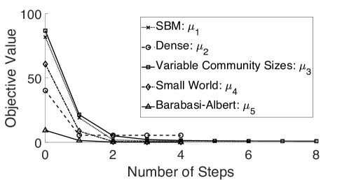
Figure 2: Verification of convex objective

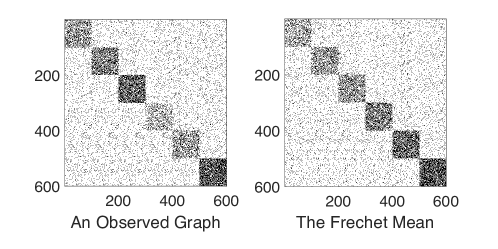
Figure 3: Visual comparison between an observation from $\mu_{1}$ and the approximate Fréchet mean of $\mu_{1}$

Fréchet mean. An example of such a dataset could be a temporal set in which the node labels are consistent across all the graphs.

Due to the mislabeling of nodes, a better graphic to visually inspect the quality of the estimate in theorem 1 is to compare the spectra of the observed graphs versus the spectra of the empirical Fréchet mean. In figure 4 below, we compute the euclidean average of the observed spectra from the graphs in $M_{1}$. We then determine the Fréchet mean graph as described in algorithm 2 and compute the histogram of its spectra. The histogram of spectral values for random matrices is discussed throughout the works of [3, 34, 33, 8, 37]. Overlaying the average histogram from the observed set and the histogram of $G_{N}^{*}$ gives a sense as to how well the approximation recovers the euclidean averaged eigenvalues.

Figure 4 shows that by capturing the behavior of the largest eigenvalues, as guaranteed by theorem 1, we exactly recover the entire distribution of the set of graphs as is shown by the alignment of the distribution of the extremal and bulk eigenvalues. This result suggest that the largest eigenvalues of the stochastic block model completely characterize the models behavior.

8.3 Dense Empirical Fréchet Mean

In an obvious extension of the theory, we attempt to understand the consequences that arise when given a sample of dense graphs. The probability measure, $\mu_{2}$, for this section has an expected density

$$\mathbb{E}\left[\rho|\mu_{2}\right]>\frac{\ln^{3}(n)}{n}.$$ (59)

In fig. 5 we display the adjacency matrix of an arbitrary graph from the set $M_{2}$ and the adjacency matrix of the estimated empirical Fréchet mean $G_{N}^{*}$.

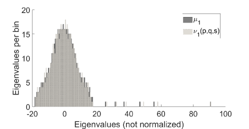
Figure 4: Average histogram of spectra from $M_{1}$ overlayed by histogram of spectra from $\mathop{\mathfrak{F}}(\nu_{1})$

Figure 5: Visual comparison between an observation from $\mu_{2}$ and the approximate Fréchet mean of $\mu_{2}$

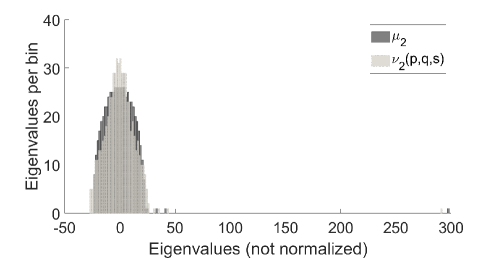
Figure 6: Average histogram of spectra from $M_{2}$ overlayed by histogram of spectra from $\mathop{\mathfrak{F}}(\nu_{2})$

Figure 5 illustrates the obvious distinction between the visualization of the adjacency matrix of the empirical Fréchet mean and an arbitrary adjacency matrix of a graph from $M_{2}$. This distinction is expected since the average of a set need not resemble any one element of the set in theory. In addition, the only guarantee from theorem 1 is that the extremal eigenvalues of the empirical Fréchet mean matches the average of the extremal eigenvalues of the graphs in the dataset. In figure 6 we again plot the average histograms of the observed graphs against the histogram of the empirical Fréchet mean as in section 8.2. In figure 2 we saw that the objective did not decay to zero so we do not expect a perfect alignment of the extremal eigenvalues in figure 6. Figure 6 shows the misalignment of the largest eigenvalue of the empirical Fréchet mean from the average largest eigenvalue of the graphs in the dataset $M_{2}$. This misalignment could be due to the graphs in the dataset being too dense which is well known to be related to the magnitude of the largest eigenvalue for a graph.

8.4 Variable Community Sizes in Stochastic Block Models

While we introduce stochastic block models for variably sized communities, the practical applications of the theory resulted in restricting the class of stochastic block models in our search space to those with equal sized communities with at most one larger community. Nonetheless, a stochastic block model with variably sized communities can be approximated by a stochastic block model with equal sized communities just as well. In this section we explore this idea. While we see clear distinctions between the visualization of the adjacency matrices in figure 7, the alignment of the extremal eigenvalues remains accurate as is shown in figure 8. The distinction then comes from the distribution of the bulk eigenvalues.

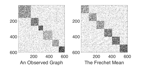
Figure 7: Visual comparison between an observation from $\mu_{3}$ and the approximate Fréchet mean of $\mu_{3}$

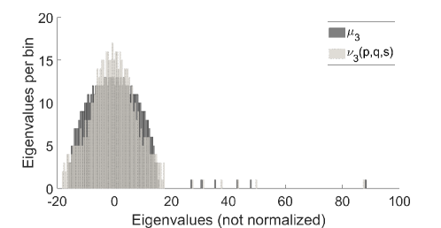
Figure 8: Average histogram of spectra from $M_{3}$ overlayed by histogram of spectra from $\mathop{\mathfrak{F}}(\nu_{3})$

Both of these figures suggest further research into the effect of community size and community strength on the extremal eigenvalues of a stochastic block model. It is worth noting that the extremal eigenvalues of stochastic block models are not solely dictated by the vector of community strengths $\bm{p}$ which suggests there exists sets of parameters $(\bm{p}_{1},q_{1},\bm{s}_{1})$ and $(\bm{p}_{2},q_{2},\bm{s}_{2})$ such that $(\bm{p}_{1},q_{1},\bm{s}_{1})\neq(\bm{p}_{2},q_{2},\bm{s}_{2})$ but $\sigma_{c}(\mathop{\mathfrak{F}}(\mu_{{\mathop{\scriptscriptstyle\mathrm{SBM}}}}(\bm{p}_{1},q_{1},\bm{s}_{1})))=\sigma_{c}(\mathop{\mathfrak{F}}(\mu_{{\mathop{\scriptscriptstyle\mathrm{SBM}}}}(\bm{p}_{2},q_{2},\bm{s}_{2}))).$ This is noteworthy as it implies that within the class of stochastic block models with variable community sizes, the solution to (36) is not unique. If we instead had utilized a distance that measured the distribution of the bulk eigenvalues a unique solution would likely exist though this idea is not explored in this paper.

8.5 Small World Empirical Fréchet Mean

The probability measure in this section is associated with the small world ensemble where the number of connected nearest neighbors is $K=22$ and the probability of rewiring is $\beta=0.7$. Figure 9 gives a visualization of the approximation performed by the stochastic block model ensemble.

One interpretation of figure 9 is to think of the stochastic block model kernel as a blockwise constant approximation of a kernel for $\mu_{4}$. This interpretation is related to the work done in [27] which motivated much of the theory in this paper.

In figure 10 we again overlay the histograms of the graphs we consider. Notice that the histogram of eigenvalues of the Fréchet mean of the stochastic block model approximation, $\nu_{4}$ seemingly has eigenvalues outside of the bulk on the left as well as to the right. One potential cause of this phenomenon could be that the large number of communities leads to a slower convergence to the generalized “semi-circle” law, see discussion of this in [3], and a larger graph is needed to get a better estimation of the histogram over the bulk.

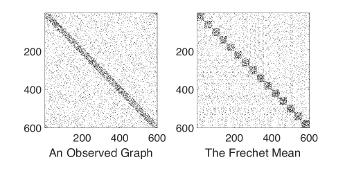
Figure 9: Visual comparison between an observation from $\mu_{4}$ and the approximate Fréchet mean of $\mu_{4}$

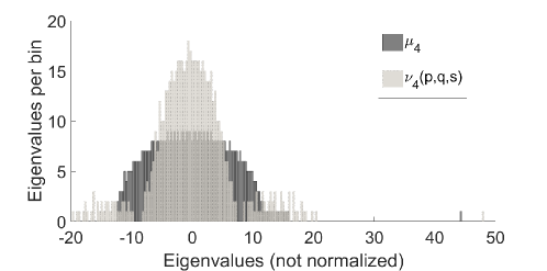
Figure 10: Average histogram of spectra from $M_{4}$ overlayed by histogram of spectra from $h(\nu_{4})$

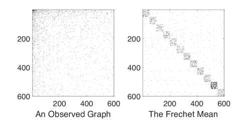
Figure 11: Visual comparison between an observation from $\mu_{5}$ and the approximate Fréchet mean of $\mu_{5}$

Regardless of this we observe obvious visual similarities between the empirical Fréchet mean and an arbitrary graph in the observed set $M_{4}$.

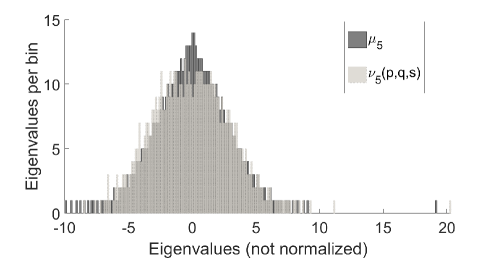
Figure 12: Average histogram of spectra from $M_{5}$ overlayed by histogram of spectra from $\mathop{\mathfrak{F}}(\nu_{5})$

8.6 Barabasi-Albert Empirical Fréchet Mean

The probability measure in this section is associated with a Barabasi-Albert ensemble. The initial graph for the ensemble is fully connected on $m_{0}=5$ nodes and $m=5$ edges were added at each step. In figure 11 we reorder the nodes based on their degree for the Barabasi-Albert graph to get a better visual understanding of the similarities between an observed graph and the Fréchet mean. The estimate for the number of communities from algorithm 1 is $c^{*}=12$ resulting in $50$ vertices per community.

Figure 12 again depicts the alignment of the spectra from the approximate Fréchet mean with that of the average spectra of the graphs from set $M_{5}$. Note the misalignment in the largest eigenvalues could be due to the finite graph approximation. Recall all results hold in the limit of large graph size but throughout all of these experiments we are approximating infinite graphs with finite graphs in addition to making the approximation by the stochastic block model ensemble.

8.7 Application to regression

This subsection is focused on performing a simplified experiment addressing the theory presented in section 7. We first generate a synthetic data set of graphs by allowing the parameters of the stochastic block model to vary with time. For simplicity we hold $q$ and the non-zero entries of $\bm{s}$ fixed as

$$\bm{s}(t)=\begin{bmatrix}1/3\\ 1/3\\ 1/3\\ 0\\ \vdots\end{bmatrix},q=0.08.$$ (60)

For $t\in[0,1]$ we let the non-zero entries of $\bm{p}$ vary linearly as

$$\bm{p}(t)=\begin{bmatrix}0.1+0.1t\\ 0.2+0.15t\\ 0.35+0.2t\\ 0\\ \vdots\end{bmatrix}.$$ (61)

For $T\sim unif(0,1)$, the distribution over $\mathcal{G}$ is given as $\mu_{{\mathop{\scriptscriptstyle\mathrm{SBM}}}}(\bm{p}(T),q,\bm{s})$. For each sample from $unif(0,1)$ there is a corresponding sample from the stochastic block model. By construction we know the number of communities in the observed graphs will be constant at $c^{*}=3$ dictating the number of non-zero entries of $\bm{p}$ we allow to vary when searching for a solution to equation (52).

Figure 13: Regression for Stochastic Block Models

We take $N=30$ samples for the sample set $M=\{(t_{i},G_{i})\}_{i=1}^{30}$ in the experiment. In an effort of visualization, since we are unable to plot a graph $G$ on the y-axis, we plot the estimated values $\bm{p}^{*}(t)$ at new time points. We expect to recover the lines that define $\bm{p}(t)$ for time values that were not sampled. Below we mark the estimated values of parameters for 6 graphs at the times $t\in\{0,0.2,0.4,0.6,0.8,1\}$ with a $\times$. A vertical line in figure 13 indicates the three entries of $\bm{p}^{*}(t)$.

The true parameter values for the sampled graphs are displayed for comparison with the estimated values of the parameters at new times. In practice, the true values are unknown to us without a significant amount of work and we would only be able to display the recovered parameter values. A problem with this approach is that for each new time point, the corresponding Fréchet mean must be found. This is incredibly costly since the evaluation of the objective involves solving a minimization problem at each time point. We address this issue in forthcoming papers by performing regression on the recovered parameter values after determining a few Fréchet means at select time points.

9 Conclusion

In the area of statistical analysis of for graph valued data, determining an average graph is a point of priority among researchers. The standard practice in the field is to utilize the most central graph among the observed set of graphs as a makeshift Fréchet mean. Throughout this paper, we have shown that when considering the metric $d_{A_{c}}$ it is possible to determine an approximation to the empirical Fréchet mean given a dataset of sparse graphs.

How this approximate Fréchet mean is utilized is up to the discretion of the researcher however in section 7 we explore one motivating idea that utilizes the Fréchet mean, termed Fréchet regression in the work in [29]. This is but one example of the utility of the Fréchet mean graph, another interesting application of this graph is to further push the work in [25] which introduces a centered random graph model to capture the variance of a set of observations around a mean graph.

Beyond the applicability of the Fréchet mean, theorem 2 identifies a set of graphs that is dense, in the large graph limit and with respect to $d_{A_{c}}$, in the set of sparse graphs. This result is useful in many respects as now we may “project” (in some sense of the term) any large sparse graph onto the set of Fréchet means of stochastic block models and begin to understand its structure as captured by the largest $c$ eigenvalues. This representation of a graph by the Fréchet mean of a stochastic block model can be seen as a $2c+1$ dimensional approximately invertible embedding of a graph where the embedding is the the $c$ non-zero entries of $\bm{p}$ and $\bm{s}$ and the parameter $q$. This embedding furthermore allows for natural analysis in the parameter space of the stochastic block model ensemble rather than analysis in $\mathcal{G}$.

Appendix A Classic Results

A.1 Universality of the Stochastic Block Model with respect to the 2-norm

Theorem 3 ([27])

Let $\mu_{g}$ be a probability measure with kernel function $g:[0,1]^{2}\mapsto(0,1)$ such that $g$ is H$\ddot{o}$lder-continuous with expected density

$$\mathbb{E}\left[\rho_{n}\right]=\Omega\left(\frac{\ln^{3}(n)}{n}\right).$$ (62)

Let $\mathcal{T}$ be the set of bijective functions on the interval $[0,1]$. For any $\varepsilon>0$, there exists a kernel $f(x,y;\bm{p},q,\bm{s})$ for a stochastic block model with the following properties:

• $\bm{s}$ has $c$ non-zero entries

• $\bm{s}(1)\geq\bm{s}(i)$ for $i=1,2,...,c$

• $\bm{s}(i)=\bm{s}(j)$ for $i,j=2,...,c$

such that

$$d_{k}(g(x,y),f(x,y;\bm{p},q,\bm{s}))=\underset{\tau\in\mathcal{T}}{\text{inf }}\int\int_{(0,1)^{2}}\left|g(\tau(x),\tau(y))-f(x,y;\bm{p},q,\bm{s})\right|^{2}dxdy\leq\varepsilon$$ (63)

Proof of Theorem 3

The proof can be found in [27].

The theorem states that the class of kernels that generate sparse graphs in expectation can be approximated by a kernel from the class of stochastic block models when we allow for the correct $\tau$ on the interval $[0,1]$. The choice of $\tau$ is interpreted as a relabeling of the nodes.

A.2 Expected Value of the Largest Eigenvalues of a Stochastic Block Model

Theorem 4 ([8])

Given kernel $f(x,y;\bm{p},q,\bm{s})\in K_{{\mathop{\scriptscriptstyle\mathrm{SBM}}}}$ with probability measure $\mu_{{\mathop{\scriptscriptstyle\mathrm{SBM}}}}$ such that $\bm{s}$ has $c$ non-zero entries. Let $G_{\mu_{{\mathop{\scriptscriptstyle\mathrm{SBM}}}}}$ be a random graph with adjacency matrix $\bm{A}$. In the limit of large graph size, let $\bm{\lambda}^{\bm{E}}=\mathbb{E}\left[\sigma(\bm{A})\right]$. For $k=1,...,c$, the $k^{th}$ largest eigenvalue, $\bm{\lambda}^{\bm{E}}(k)$, is the unique root of

$$f_{k}(z)=1+\bm{\lambda}_{\bm{E}}(k)\{R(\bm{v}_{k},\bm{v}_{k},z)-R(\bm{v}_{k},\bm{V}_{-k},z)[(D_{-k})^{-1}+R(\bm{V}_{-k},\bm{V}_{-k},z)]^{-1}\times R(\bm{V}_{-k},\bm{v}_{k},z)\}$$ (64)

in the interval $[a_{k},b_{k}]$ where

$$a_{k}=\begin{cases}\frac{\bm{\lambda}_{\bm{E}}(k)}{1+c_{0}/2}\quad\bm{\lambda}_{\bm{E}}(k)>0\\ \frac{1+c_{0}/2}{\bm{\lambda}_{\bm{E}}(k)}\quad\bm{\lambda}_{\bm{E}}(k)<0\end{cases}\quad b_{k}=\begin{cases}\frac{1+c_{0}/2}{\bm{\lambda}_{\bm{E}}(k)}\quad\bm{\lambda}_{\bm{E}}(k)>0\\ \frac{\bm{\lambda}_{\bm{E}}(k)}{1+c_{0}/2}\quad\bm{\lambda}_{\bm{E}}(k)<0\end{cases}$$ (65)

Asymptotically,

$$f_{k}(z)=1+\bm{\lambda}_{\bm{E}}(k)R(\bm{v}_{k},\bm{v}_{k},z)+H.O.T.$$ (66)

Here $\bm{\lambda}_{\bm{E}}=\sigma(\mathbb{E}\left[\bm{A}\right])$ and $\bm{\lambda}_{\bm{E}}(k)$ is the $k^{th}$ largest eigenvalue while $\bm{v}_{k}$ denotes the associated eigenvector. $\bm{V}$ is the $n\times c$ matrix of orthonormal eigenvectors of $\mathbb{E}\left[\bm{A}\right]$ and $\bm{V}_{-k}$ is the submatrix of $\bm{V}$ with the $k^{th}$ column and row removed. $\bm{D}$ is the diagonal matrix of eigenvalues of $\mathbb{E}\left[\bm{A}\right]$ organized in decreasing order. $\bm{D}_{-k}$ is the submatrix of $\bm{D}$ with the $k^{th}$ column and row removed.

$$R(M_{1},M_{2},z)=-\sum_{l=0,l\neq 1}^{L}z^{-(l+1)}M_{1}^{T}\mathbb{E}\left[\bm{W}^{l}\right]M_{2}$$ (67)

where $\bm{W}=\bm{A}-\mathbb{E}\left[\bm{A}\right]$ and $L=4$ is typically sufficient and $c_{0}\in(0,1)$.

Proof of Theorem 4

The proof can be found in [8].

This result gives an expression to determine the expected eigenvalues of graphs drawn from the stochastic block model ensemble. As suggested in [8], the roots of $f_{k}(z)$ can be found using Newton’s method.

A.3 Convergence of Spectrum to Operator Spectrum

Theorem 5

Given a canonical kernel $f(x,y;\bm{p},q,\bm{s})\in K_{{\mathop{\scriptscriptstyle\mathrm{SBM}}}}$ with probability measure $\mu_{{\mathop{\scriptscriptstyle\mathrm{SBM}}}}$ such that $\bm{s}$ has $c$ non-zero entries. Let $G_{\mu_{{\mathop{\scriptscriptstyle\mathrm{SBM}}}}}$ be a random graph with adjacency matrix $\bm{A}$. For equispaced points $\{\xi_{i}\}_{i=1}^{n}$ in the interval $[0,1]$, define the expected adjacency matrix as

$$\mathbb{E}\left[\bm{A}\right]=f(\xi_{i},\xi_{j};\bm{p},q,\bm{s}).$$ (68)

Denote the spectrum of the expected adjacency matrix by vector in $\operatorname{\mathbb{R}}^{n}$ as

$$\sigma(\mathbb{E}\left[\bm{A}\right])=\bm{\lambda}_{\bm{E}}$$ (69)

where $\bm{\lambda}_{\bm{E}}$ is sorted in descending order. Define the linear integral operator with kernel $f$, $L_{f}:L^{2}([0,1])\mapsto L^{2}([0,1])$ as

$$L_{f}(g(x))=\int_{0}^{1}f(x,y;\bm{p},s,\bm{s})g(y)dy.$$ (70)

Denote the spectrum of the linear integral operator as

$$\sigma(L_{f})=\bm{\lambda}_{L_{f}}$$ (71)

where $\bm{\lambda}_{L_{f}}$ is sorted in descending order and indexed by $i$.

$$\lim_{n\to\infty}\frac{1}{\sqrt{n}}\bm{\lambda}_{E}(i)=\bm{\lambda}_{L_{f}}(i)$$ (72)

Proof of Theorem 5

This theorem is shown in each of [32, 14, 6, 20] but has been adapted to the notations of this paper. The interpretation of this result is that in the limit of large graph size, we may approximate the spectrum of the operator associated with a stochastic block model by the eigenvalues of the discretized operator when appropriately normalized.

A.4 Weyl-Lidskii

Theorem 6

Let $H$ be a self-adjoint linear operator on a Hilbert space $\mathcal{H}$. Let $A$ be a bounded operator on $\mathcal{H}$. Then

$$\sigma(H+A)\subset\left\{\lambda:dist(\lambda,\sigma(H))\leq||A||\right\}$$ (73)

Proof of Theorem 6

These are standard bounds that can be found in many good books on matrix perturbation theory (e.g., [31]).

A.5 Extremal Eigenvalues of graphs from stochastic block models are normally distributed

Theorem 7

Given kernel $f(x,y;\bm{p},q,\bm{s})\in K_{{\mathop{\scriptscriptstyle\mathrm{SBM}}}}$ with probability measure $\mu_{{\mathop{\scriptscriptstyle\mathrm{SBM}}}}$ such that $\bm{s}$ has $c$ non-zero entries. Let $G_{\mu_{{\mathop{\scriptscriptstyle\mathrm{SBM}}}}}$ be a random graph with adjacency matrix $\bm{A}$. In the limit of large graph size, the $c$ largest eigenvalues of $A$, denoted $\bm{\lambda}(i)$, for $i=1,...,c$ converges in distribution to a normal distribution

$$\bm{\lambda}(i)\sim N(m_{i},v_{i})$$ (74)

with mean $m_{i}$ and finite variance $v_{i}$.

Proof of Theorem 7

We note that the mean $m_{i}$ is related to the eigenvalues of the expected adjacency matrix by way of theorem 4.

Appendix B There exists a continuous map, $\tau_{k}$, from the extremal eigenvalues of $\sigma(\mathbb{E}\left[A\right])$ to the extremal eigenvalues of $\mathbb{E}\left[\sigma(A)\right]$

Theorem 8

Given kernel $f(x,y;\bm{p},q,\bm{s})\in K_{{\mathop{\scriptscriptstyle\mathrm{SBM}}}}$ with probability measure $\mu_{{\mathop{\scriptscriptstyle\mathrm{SBM}}}}$ such that $\bm{s}$ has $c$ non-zero entries. Let $G_{\mu_{{\mathop{\scriptscriptstyle\mathrm{SBM}}}}}$ be a random graph with adjacency matrix $\bm{A}$. For equispaced points $\{\xi_{i}\}_{i=1}^{n}$ in the interval $[0,1]$, define the expected adjacency matrix as

$$\mathbb{E}\left[\bm{A}\right]=f(\xi_{i},\xi_{j};\bm{p},q,\bm{s}).$$ (75)

Denote the spectrum of the expected adjacency matrix by a vector in $\operatorname{\mathbb{R}}^{n}$ as

$$\sigma(\mathbb{E}\left[\bm{A}\right])=\bm{\lambda}_{\bm{E}}$$ (76)

where $\bm{\lambda}_{\bm{E}}$ is sorted in descending order. Denote the expected spectrum of the adjacency matrix by a vector in $\operatorname{\mathbb{R}}^{n}$ as

$$\mathbb{E}\left[\sigma(\bm{A})\right]=\bm{\lambda}^{\bm{E}}$$ (77)

where $\bm{\lambda}^{\bm{E}}$ is sorted in descending order. In the limit of large graph size, there exist $c$ continuous maps $\tau_{k}$ such that

$$\tau_{k}(\bm{\lambda}_{\bm{E}}(k))=\bm{\lambda}^{\bm{E}}(k)\quad k=1,...,c.$$ (78)

Proof of Theorem 8

We need only prove for any general $k$. Let $f_{k}(z)=1+\bm{\lambda}_{\bm{E}}(k)R(\bm{v}_{k},\bm{v}_{k},z)$ from theorem 4. Note that $\bm{\lambda}_{\bm{E}}(k)$ depends continuously on the parameters of the kernel function, $\bm{p},q,\bm{s}$ since the spectrum is continuous with respect to the kernel function. Furthermore, $\bm{v}_{k}(i)$ depends continuously on the parameters $\bm{p},q,\bm{s}$ for all $i=1,...,c$. This implies that $f_{k}(z)$ is continuous in the interval $[a_{k},b_{k}]$ where $a_{k},b_{k}$ are as defined in theorem 4. Therefore $f_{k}(z)$ may be approximated by a polynomial $p_{k}(z)$ with coefficients $\bm{c}$ such that $\bm{c}(i)$ depends continuously on the parameters $\bm{p},q,\bm{s}$. As a result, the roots of $f_{k}(z)$ depend continuously on the parameters $\bm{p},q,\bm{s}$ since the roots of the polynomials $p_{k}(z)$ depend continuously on the parameters.

Appendix C The spectra of linear integral operators are close if and only if the kernels are close

Theorem 9

Let $f$ be the kernel for probability measure $\mu$ and $f_{{\mathop{\scriptscriptstyle\mathrm{SBM}}}}\in K_{{\mathop{\scriptscriptstyle\mathrm{SBM}}}}$ be the kernel for probability measure $\mu_{{\mathop{\scriptscriptstyle\mathrm{SBM}}}}$. Let $L_{f}$ and $L_{f_{{\mathop{\scriptscriptstyle\mathrm{SBM}}}}}$ be the linear integral operators with kernels $f$ and $f_{{\mathop{\scriptscriptstyle\mathrm{SBM}}}}$ acting on $\mathcal{L}^{2}([0,1])$ defined below as

$$L_{f}(g(x))=\int_{0}^{1}f(x,y)g(y)dy$$ (79)

$$L_{f_{{\mathop{\scriptscriptstyle\mathrm{SBM}}}}}(g(x))=\int_{0}^{1}f_{{\mathop{\scriptscriptstyle\mathrm{SBM}}}}(x,y;\bm{p},q,\bm{s})g(y)dy$$ (80)

Let $\varepsilon>0$. Assume

$$||f(x,y)-f_{{\mathop{\scriptscriptstyle\mathrm{SBM}}}}(x,y;\bm{p},q,\bm{s})||_{2}<\varepsilon\implies||\sigma(L_{f})-\sigma(L_{f_{{\mathop{\scriptscriptstyle\mathrm{SBM}}}}})||_{2}<\frac{25}{4}\varepsilon$$ (81)

Proof of Theorem 9

The approach is to first show that the linear integral operator, $L_{k}$, with kernel $k(x,y)=f(x,y)-f_{{\mathop{\scriptscriptstyle\mathrm{SBM}}}}(x,y;\bm{p},q,\bm{s})$ has a norm controlled by $\varepsilon$. We then show that the eigenvalues of $L_{f}$ are close to the eigenvalues of $L_{f_{{\mathop{\scriptscriptstyle\mathrm{SBM}}}}}$. We then bound the error by approximating the rate of decay in the tail of the spectrum and controlling the first finite number of terms by $\varepsilon$.

Let $\varepsilon>0$ and assume that

$$||f(x,y)-f_{{\mathop{\scriptscriptstyle\mathrm{SBM}}}}(x,y;\bm{p},q,\bm{s})||_{2}<\varepsilon.$$ (82)

Let $L_{f}$ and $L_{f_{{\mathop{\scriptscriptstyle\mathrm{SBM}}}}}$ be linear integral operators with kernels $f$ and $f_{{\mathop{\scriptscriptstyle\mathrm{SBM}}}}$ respectively acting on $\mathcal{L}^{2}([0,1])$ defined as

$$L_{f}(g):=\int_{[0,1]}f(x,y)g(y)dy$$ (83)

$$L_{f_{{\mathop{\scriptscriptstyle\mathrm{SBM}}}}}(g):=\int_{[0,1]}f_{{\mathop{\scriptscriptstyle\mathrm{SBM}}}}(x,y;\bm{p},q,\bm{s})g(y)dy$$ (84)

Let $\bm{\lambda}_{f}=\sigma(L_{f})$ and $\bm{\lambda}_{f_{{\mathop{\scriptscriptstyle\mathrm{SBM}}}}}=\sigma(L_{f_{{\mathop{\scriptscriptstyle\mathrm{SBM}}}}})$ be the spectra of the operators sorted in descending order of magnitude and indexed by $i\in I$, where $I$ is an arbitrary index set. Define $k(x,y)=f(x,y)-f_{{\mathop{\scriptscriptstyle\mathrm{SBM}}}}(x,y;\bm{p},q,\bm{s})$ and the corresponding linear integral operator

$$L_{k}(g):=\int_{[0,1]}k(x,y)g(y)dy.$$ (85)

We first show that the norm of $L_{k}$ is small.

$$||L_{k}||^{2} =\underset{||g||=1}{\text{sup }}||L_{k}(g)||_{2}^{2}$$ (86)

$$=\underset{||g||=1}{\text{sup }}||\int_{0}^{1}k(x,y)g(y)dy||_{2}^{2}$$ (87)

For a fixed $x$ we have

$$\int_{0}^{1}k(x,y)g(y)dy\leq\sqrt{||k(x,y)||_{2}^{2}||g(y)||_{2}^{2}}$$ (88)

by Cauchy-Schwarz so

$$||L_{k}||^{2} \leq\underset{||g||=1}{\text{sup }}||\sqrt{||k(x,y)||_{2}^{2}||g(y)||_{2}^{2}}||_{2}^{2}$$ (89)

$$=||\text{ }||k(x,y)||_{2}||_{2}^{2}$$ (90)

$$=\int_{0}^{1}\left(\sqrt{\int_{0}^{1}k(x,y)^{2}dy}\right)dx.$$ (91)

Let $h(x)=\int_{0}^{1}k(x,y)^{2}dy$ and define the set $X=\{x\in[0,1]:h(x)<\varepsilon\}$ . Then

$$||L_{k}||^{2} \leq\int_{0}^{1}\left(\sqrt{h(x)}\right)dx$$ (92)

$$=\int_{X}\sqrt{h(x)}dx+\int_{[0,1]\backslash X}\sqrt{h(x)}dx$$ (93)

Since $f(x)=\sqrt{}$ is Lipschitz on $[\varepsilon,1]$ with Lipschitz constant $\frac{1}{2\sqrt{\varepsilon}}$ we have

$$||L_{k}||\leq\int_{X}\sqrt{h(x)}dx+\int_{[0,1]\backslash X}\frac{1}{2\sqrt{\varepsilon}}h(x)dx$$ (95)

We then have

$$||L_{k}|| \leq\int_{X}\sqrt{h(x)}dx+\int_{[0,1]\backslash X}\frac{1}{2\sqrt{\varepsilon}}h(x)dx$$ (96)

$$=\int_{X}\sqrt{h(x)}dx+\int_{[0,1]\backslash X}\frac{1}{2\sqrt{\varepsilon}}h(x)dx$$ (97)

$$\leq\int_{X}\sqrt{h(x)}dx+\int_{0}^{1}\frac{1}{2\sqrt{\varepsilon}}h(x)dx$$ (98)

$$<\sqrt{\varepsilon}+\frac{\sqrt{\varepsilon}}{2}=\frac{3}{2}\sqrt{\varepsilon}$$ (99)

Thus $||L_{k}||<\frac{3}{2}\sqrt{\varepsilon}$ which shows the norm of $L_{k}$ is controlled by $\varepsilon$.

We want to show

$$||\bm{\lambda}_{f}-\bm{\lambda}_{f_{{\mathop{\scriptscriptstyle\mathrm{SBM}}}}}||<\frac{25}{4}\sqrt{\varepsilon}.$$ (100)

Note

$$L_{f}=L_{f_{{\mathop{\scriptscriptstyle\mathrm{SBM}}}}}+L_{k}.$$ (101)

By the Weyl-Lidskii theorem,

$$|\bm{\lambda}_{f}(i)-\bm{\lambda}_{f_{{\mathop{\scriptscriptstyle\mathrm{SBM}}}}}(i)|<\frac{3}{2}\sqrt{\varepsilon}$$ (102)

since the norm of the operator $L_{k}$ is less than $\frac{3}{2}\sqrt{\varepsilon}$. Furthermore, $||\bm{\lambda}_{f}||_{2}<\infty$ and $||\bm{\lambda}_{f_{{\mathop{\scriptscriptstyle\mathrm{SBM}}}}}||_{2}<\infty$ since the operators are compact. For $n^{*}>\frac{1}{\sqrt{\varepsilon}}$ we have that

$$||\bm{\lambda}_{f}-\bm{\lambda}_{f_{{\mathop{\scriptscriptstyle\mathrm{SBM}}}}}||^{2}_{2} =\sum_{i=1}^{\infty}(\bm{\lambda}_{f}(i)-\bm{\lambda}_{f_{{\mathop{\scriptscriptstyle\mathrm{SBM}}}}}(i))^{2}$$ (103)

$$=\sum_{i=1}^{n^{*}}(\bm{\lambda}_{f}(i)-\bm{\lambda}_{f_{{\mathop{\scriptscriptstyle\mathrm{SBM}}}}}(i))^{2}+\sum_{i=n^{*}+1}^{\infty}(\bm{\lambda}_{f}(i)-\bm{\lambda}_{f_{{\mathop{\scriptscriptstyle\mathrm{SBM}}}}}(i))^{2}$$ (104)

$$\leq\sum_{i=1}^{n^{*}}(\frac{3}{2}\sqrt{\varepsilon})^{2}+\sum_{i=n^{*}+1}^{\infty}(\bm{\lambda}_{f}(i)-\bm{\lambda}_{f_{{\mathop{\scriptscriptstyle\mathrm{SBM}}}}}(i))^{2}$$ (105)

$$=\frac{9}{4}n^{*}\varepsilon+\sum_{i=n^{*}+1}^{\infty}(\bm{\lambda}_{f}(i)-\bm{\lambda}_{f_{{\mathop{\scriptscriptstyle\mathrm{SBM}}}}}(i))^{2}$$ (106)

$$=\frac{9}{4}n^{*}\varepsilon+\sum_{i=n^{*}+1}^{\infty}\bm{\lambda}_{f}^{2}(i)-2\bm{\lambda}_{f}\bm{\lambda}_{f_{{\mathop{\scriptscriptstyle\mathrm{SBM}}}}}(i)+\bm{\lambda}^{2}_{f_{{\mathop{\scriptscriptstyle\mathrm{SBM}}}}}(i)$$ (107)

Without loss of generality, we assume for $i>n^{*}$, both $\bm{\lambda}_{f}(i)<\frac{1}{i}$ and $\bm{\lambda}_{f_{{\mathop{\scriptscriptstyle\mathrm{SBM}}}}}(i)<\frac{1}{i}$. We therefore have a loose bound on the tails of the sequences of eigenvalues. Thus

$$||\bm{\lambda}_{f}-\bm{\lambda}_{f_{{\mathop{\scriptscriptstyle\mathrm{SBM}}}}}||^{2}_{2} \leq\frac{9}{4}n^{*}\varepsilon+\sum_{i=n^{*}+1}^{\infty}\frac{1}{i^{2}}+2\frac{1}{i^{2}}+\frac{1}{i^{2}}$$ (108)

$$=\frac{9}{4}\varepsilon^{1/2}\varepsilon+4\varepsilon^{1/2}$$ (109)

$$=\frac{25}{4}\sqrt{\varepsilon}$$ (110)

This shows the forward direction. The backwards direction is a direct result from the theory of Hilbert-Schmidt operators. Let $f_{1}$ and $f_{2}$ be two kernels of linear integral operators defined as

$$L_{f_{1}}=\int_{0}^{1}f_{1}(x,y)g(y)dy$$ (111)

$$L_{f_{2}}=\int_{0}^{1}f_{2}(x,y)g(y)dy$$ (112)

where $f_{1}$ and $f_{2}$ are symmetric. Let $\sigma(L_{f_{1}})=\bm{\lambda}_{1}$ and $\sigma(L_{f_{2}})=\bm{\lambda}_{2}$ be the spectra of $L_{f_{1}}$ and $L_{f_{2}}$ respectively sorted in descending order. Assume that

$$||\bm{\lambda}_{1}-\bm{\lambda}_{2}||_{2}^{2}<\varepsilon$$ (113)

We want to show that

$$||f_{1}-f_{2}||_{2}^{2}<\varepsilon$$ (114)

Note $||L_{f_{1}}||_{HS}=\sum_{i=1}^{\infty}\bm{\lambda}_{1}(i)^{2}$ and that $||L_{f_{1}}||_{HS}=||f_{1}||_{2}^{2}$. As a consequence

$$||f_{1}||_{2}^{2}=\sum_{i=1}^{\infty}\bm{\lambda}_{1}(i)^{2}.$$ (115)

Similarly,

$$||f_{2}||_{2}^{2}=\sum_{i=1}^{\infty}\bm{\lambda}_{2}(i)^{2}.$$ (116)

Thus

$$||f_{1}-f_{2}||_{2}^{2}=\sum_{i=1}^{\infty}(\bm{\lambda}_{1}(i)-\bm{\lambda}_{2}(i))^{2}=||\bm{\lambda}_{1}-\bm{\lambda}_{2}||_{2}^{2}<\varepsilon.$$ (117)

$\square$

The work in [27] states that we may approximate a certain class of kernel probability measures by stochastic block model kernels, $K_{{\mathop{\scriptscriptstyle\mathrm{SBM}}}}$. We have shown that in doing so, we may also measure distances with respect to $d_{A}$ and maintain that the spectra of the expected adjacency matrices remain close. We also will need to show that for a small change in the spectra of the linear integral operators, the respective kernels remain close in the metric $d_{k}$.

Appendix D The Fréchet mean of graphs from the stochastic block model is the expected spectrum

Theorem 10

Given a canonical kernel $f(x,y;\bm{p},q,\bm{s})\in K_{{\mathop{\scriptscriptstyle\mathrm{SBM}}}}$ for probability measure $\mu_{{\mathop{\scriptscriptstyle\mathrm{SBM}}}}$ such that $\bm{s}$ has $c$ non-zero entries. Let $G_{\mu_{{\mathop{\scriptscriptstyle\mathrm{SBM}}}}}$ be a random graph with adjacency matrix $\bm{A}$. Let

$$\bm{\lambda}^{*}_{{\mathop{\scriptscriptstyle\mathrm{SBM}}}}=\sigma(\underset{G\in M}{\text{argmin }}\mathbb{E}\left[d_{A_{c}}^{2}(G,G_{\mu_{{\mathop{\scriptscriptstyle\mathrm{SBM}}}}})\right])$$ (118)

$$\bm{\lambda}^{\bm{E}}=\mathbb{E}\left[\sigma(G_{\mu_{{\mathop{\scriptscriptstyle\mathrm{SBM}}}}})\right]$$ (119)

In the limit of large graph size, for $i=1,...,c$

$$\bm{\lambda}^{*}_{{\mathop{\scriptscriptstyle\mathrm{SBM}}}}(i)=\bm{\lambda}^{\bm{E}}(i).$$ (120)

Proof of Theorem 10

The extremal eigenvalues of the adjacency matrix follow a normal distribution by theorem 7. The Fréchet mean of a normally distributed random variable is the same as its expected value. The conclusion follows. $\square$

Appendix E Density of Fréchet means of stochastic block models in the space of sparse graphs

Theorem 11

Density of Fréchet means of stochastic block models
(Theorem 2 in the main paper)
Let $\operatorname{\mathcal{M}}_{{\mathop{\scriptscriptstyle\mathrm{SBM}}}}(\mathcal{G})\subset\operatorname{\mathcal{M}}$ denote the subset of distributions associated with stochastic block models. In the limit of large graph size, $\forall$ $G\in\mathcal{G}_{s}$, $\forall$ $\varepsilon>0$, there exists $\mu_{{\mathop{\scriptscriptstyle\mathrm{SBM}}}}\in\operatorname{\mathcal{M}}_{{\mathop{\scriptscriptstyle\mathrm{SBM}}}}(\mathcal{G})$ such that

$$d_{A_{c}}(G,\mathop{\mathfrak{F}}(\mu_{{\mathop{\scriptscriptstyle\mathrm{SBM}}}}))<\varepsilon$$ (121)

Proof of Theorem 11

By theorem 3, for any kernel probability measure with the appropriate sparsity, we may find a kernel from $K_{{\mathop{\scriptscriptstyle\mathrm{SBM}}}}$ that approximates it. By theorem 9, if the kernels are close then the spectra of the induced linear integral operators are close. By theorem 8 there is a continuous map from the spectra of the expected adjacency matrix to the expected spectra of the adjacency matrix. By theorem 10 the Fréchet mean of the stochastic block model is the graph that achieves $\mathbb{E}\left[\sigma(G_{\mu_{{\mathop{\scriptscriptstyle\mathrm{SBM}}}}})\right]$. Any sparse graph $G$ may be written as $\mathop{\mathfrak{F}}(\mu)$ for a certain probability measure $\mu$. Since $\mu$ may be approximated by $\mu_{{\mathop{\scriptscriptstyle\mathrm{SBM}}}}$ we may estimate $\mathop{\mathfrak{F}}(\mu)$ as $\mathop{\mathfrak{F}}(\mu_{{\mathop{\scriptscriptstyle\mathrm{SBM}}}})$. $\square$

Appendix F A sample statistic to approximate the Fréchet mean of a stochastic block model with high probability

Theorem 12

Let $\mu_{{\mathop{\scriptscriptstyle\mathrm{SBM}}}}\in\operatorname{\mathcal{M}}_{{\mathop{\scriptscriptstyle\mathrm{SBM}}}}(\mathcal{G})$. Let $M=\{G_{i}\}_{i=1}^{N}$ be an iid sample distributed according to $\mu_{{\mathop{\scriptscriptstyle\mathrm{SBM}}}}$. Define

$$S_{N}=\underset{G\in M}{\mathrm{argmin}\text{ }}\sum_{i=1}^{N}d_{A_{c}}^{2}(G,G_{i})$$ (122)

In the limit of large system size, for every $\varepsilon$ and $\delta$, there exists an $N$ such that

$$P(d_{A_{c}}(S_{N}-\mathop{\mathfrak{F}}(\mu(\bm{p},q;c))<\delta)>1-\varepsilon$$ (123)

Proof of Theorem 12

By theorem 7 the $c$ largest eigenvalues of the stochastic block models are normally distributed with finite variance. Therefore we only need to show this result for normal random variables in $\operatorname{\mathbb{R}}^{c}$. Let $M=\{\bm{x}_{i}\}_{i=1}^{N}$ be an iid sample from a normal distribution with mean $\bm{\mu}$ and covariance $\sigma$. Let $S_{N}=\underset{\bm{x}\in M}{\text{argmin }}\sum_{i=1}^{N}||\bm{x}_{i}-\bm{x}||.$ Note that the Fréchet mean of a normal distribution is its expectation. Condiser,

$$P(||S_{N}-\bm{\mu}||<\delta)=1-P(||S_{N}-\bm{\mu}||>\delta).$$ (124)

$P(||S_{N}-\bm{\mu}||>\delta)$ states that every element in $M$ is at least $\delta$ away from the mean. Let $p=P(||\bm{x}_{1}-\bm{\mu}||>\delta)$. Then

$$1-P(||S_{N}-\bm{\mu}||>\delta)=1-P(||\bm{x}_{1}-\bm{\mu}||>\delta)^{N}=1-p^{N}.$$ (125)

Since $0\leq p<1$ then for any $\varepsilon$ we need only to pick $N$ such that

$$1-p^{N}>1-\varepsilon.$$ (126)

Taking $N>\frac{\ln(\varepsilon)}{\ln p}$ guarantees the result. Note that the dependence on $\delta$ is suppressed in the probability $p$ which implicitly depends on $\delta$. We have shown the conclusion for normally distributed random variables and since the extremal eigenvalues of stochastic block models are normally distributed, by theorem 7, the conclusion follows. $\square$

References

- [1] Abbe, E. Community detection and stochastic block models: recent developments. The Journal of Machine Learning Research 18, 1 (2017), 6446–6531.
- [2] Ambrosio, L., Gigli, N., and Savare, G. Gradient Flows: In Metric Spaces and in the Space of Probability Measures. Birkhauser Basel, Basel, Switzerland, 2008.
- [3] Avrachenkov, K., Cottatellucci, L., and Kadavankandy, A. Spectral properties of random matrices for stochastic block model. In 2015 13th International Symposium on Modeling and Optimization in Mobile, Ad Hoc, and Wireless Networks (WiOpt) (2015), pp. 537–544.
- [4] Baldesi, L., Markopoulou, A., and Butts, C. T. Spectral graph forge: Graph generation targeting modularity. CoRR abs/1801.01715 (2018).
- [5] Borgs, C., Chayes, J. T., Cohn, H., and Lovász, L. M. Identifiability for graphexes and the weak kernel metric. In Building Bridges II. Springer, 2019, pp. 29–157.
- [6] Borgs, C., Chayes, J. T., Lovász, L., Sós, V. T., and Vesztergombi, K. Convergent sequences of dense graphs ii. multiway cuts and statistical physics. Annals of Mathematics 176, 1 (2012), 151–219.
- [7] Boria, N., Negrevergne, B., and Yger, F. Fréchet Mean Computation in Graph Space through Projected Block Gradient Descent. In ESANN 2020 (Bruges, France, 2020).
- [8] Fan, J., Fan, Y., Han, X., and Lv, J. Asymptotic theory of eigenvectors for large random matrices, 2019.
- [9] Farkas, I. J. Spectra of “real-world” graphs: Beyond the semicircle law. Physical Review E 64, 2 (2001).
- [10] Ferrer, M., Serratosa, F., and Sanfeliu, A. Synthesis of Median Spectral Graph, vol. 3523. Springer Berlin Heidelberg, Berlin, Heidelberg, 2005, pp. 139–146.
- [11] Ferrer, M., Valveny, E., Serratosa, F., Riesen, K., and Bunke, H. Generalized median graph computation by means of graph embedding in vector spaces. Pattern Recognition 43, 4 (2010), 1642–1655.
- [12] Flaxman, A., Frieze, A., and Fenner, T. High degree vertices and eigenvalues in the preferential attachment graph. In Approximation, Randomization, and Combinatorial Optimization.. Algorithms and Techniques: 6th International Workshop on Approximation Algorithms for Combinatorial Optimization Problems, APPROX 2003 and 7th International Workshop on Randomization and Approximation Techniques in Computer Science, RANDOM 2003, Princeton, NJ, USA, August 24-26, 2003. Proceedings (2003), Springer Berlin Heidelberg, pp. 264–274.
- [13] Fréchet, M. Les éléments aléatoires de nature quelconque dans un espace distancié. Annales de l’institut Henri Poincaré 10, 4 (1948), 215–310.
- [14] Gao, S., and Caines, P. E. Spectral representations of graphons in very large network systems control. 2019 IEEE 58th Conference on Decision and Control (CDC) (Dec 2019).
- [15] Ginestet, C. E. Strong consistency of fréchet sample mean sets for graph-valued random variables. arXiv preprint arXiv:1204.3183 (2012).
- [16] Ginestet, C. E., Li, J., Balachandran, P., Rosenberg, S., and Kolaczyk, E. D. Hypothesis testing for network data in functional neuroimaging. The Annals of Applied Statistics 11, 2 (2017), 725–750.
- [17] Hastie, T., Tibshirani, R., and Friedman, J. The Elements of Statistical Learning. Springer Series in Statistics. Springer New York Inc., New York, NY, USA, 2001.
- [18] Jain, B. J. Statistical graph space analysis. Pattern Recognition 60 (2016), 802–812.
- [19] Jain, B. J., and Obermayer, K. Algorithms for the sample mean of graphs. In International Conference on Computer Analysis of Images and Patterns (2009), Springer, pp. 351–359.
- [20] Janson, S. Graphons, cut norm and distance, couplings and rearrangements. arXiv preprint arXiv:1009.2376 (2010).
- [21] Janson, S. Graphons, cut norm and distance, couplings and rearrangements, vol. 4 of new york journal of mathematics. NYJM Monographs, State University of New York, University at Albany, Albany, NY (2013).
- [22] Jiang, X., Munger, A., and Bunke, H. An median graphs: properties, algorithms, and applications. IEEE Transactions on Pattern Analysis and Machine Intelligence 23, 10 (2001), 1144–1151.
- [23] Le, C. M., Levina, E., and Vershynin, R. Concentration of random graphs and application to community detection. World Scientific, 2018.
- [24] Lee, J. R., Gharan, S. O., and Trevisan, L. Multiway spectral partitioning and higher-order cheeger inequalities. J. ACM 61, 6 (Dec. 2014), 37:1–37:30.
- [25] Lunagómez, S., Olhede, S. C., and Wolfe, P. J. Modeling network populations via graph distances. Journal of the American Statistical Association (2020), 1–18.
- [26] Olhede, S. C., and Wolfe, P. J. Network histograms and universality of blockmodel approximation. Proceedings of the National Academy of Sciences 111, 41 (2014), 14722–14727.
- [27] Olhede, S. C., and Wolfe, P. J. Network histograms and universality of blockmodel approximation. Proceedings of the National Academy of Sciences 111, 41 (Oct 2014), 14722–14727.
- [28] Pennec, X. Intrinsic statistics on riemannian manifolds: Basic tools for geometric measurements. Journal of Mathematical Imaging and Vision 25, 1 (2006), 127–154.
- [29] Petersen, A., and Müller, H.-G. Fréchet regression for random objects with euclidean predictors. Ann. Statist. 47, 2 (04 2019), 691–719.
- [30] Shine, A., and Kempe, D. Generative graph models based on laplacian spectra. WWW ’19: The World Wide Web Conference (05 2019), 1691–1701.
- [31] Stewart, G., and Sun, J. Matrix perturbation Theory. Academic Press, 1990.
- [32] Szegedy, B. Limits of kernel operators and the spectral regularity lemma. European Journal of Combinatorics 32, 7 (2011), 1156 – 1167. Homomorphisms and Limits.
- [33] Tang, M. The eigenvalues of stochastic blockmodel graphs, 2018.
- [34] Tao, T. Topics in random matrix theory. Graduate studies in mathematics ; v. 132. American Mathematical Society, Providence, R.I., 2012.
- [35] Wills, P., and Meyer, F. G. Metrics for graph comparison: A practitioner’s guide. PLOS ONE 15, 2 (02 2020), 1–54.
- [36] Wilson, R. C., and Zhu, P. A study of graph spectra for comparing graphs and trees. Pattern Recognition 41, 9 (2008), 2833 – 2841.
- [37] Zhu, Y. A graphon approach to limiting spectral distributions of wigner‐type matrices. Random Structures and Algorithms 56 (10 2019).