Aggregating From Multiple Target-Shifted Sources

Abstract

Multi-source domain adaptation aims at leveraging the knowledge from multiple tasks for predicting a related target domain. A crucial aspect is to properly combine different sources based on their relations. In this paper, we analyzed the problem for aggregating source domains with different label distributions, where most recent source selection approaches fail. Our proposed algorithm differs from previous approaches in two key ways: the model aggregates multiple sources mainly through the similarity of semantic conditional distribution rather than marginal distribution; the model proposes a unified framework to select relevant sources for three popular scenarios, i.e., domain adaptation with limited label on target domain, unsupervised domain adaptation and label partial unsupervised domain adaption. We evaluate the proposed method through extensive experiments. The empirical results significantly outperform the baselines.

1 Introduction

Domain Adaptation (DA) (Pan & Yang, 2009) is based on the motivation that learning a new task is easier after having learned a similar task. By learning the inductive bias from a related source domain $\mathcal{S}$ and then leveraging the shared knowledge upon learning the target domain $\mathcal{T}$, the prediction performance can be significantly improved. Based on this, DA arises in tremendous deep learning applications such as computer vision (Zhang et al., 2019; Hoffman et al., 2018b), natural language processing (Ruder et al., 2019; Houlsby et al., 2019) and biomedical engineering (Raghu et al., 2019; Wang et al., 2020).

In various real-world applications, we want to transfer knowledge from multiple sources $(\mathcal{S}_{1},\dots,\mathcal{S}_{T})$ to build a model for the target domain, which requires an effective selection and leveraging the most useful sources. Clearly, solely combining all the sources and applying one-to-one single DA algorithm can lead to undesired results, as it can include irrelevant or even untrusted data from certain sources, which can severely influence the performance (Zhao et al., 2020).

Figure 1: Limitation of merely considering marginal distribution $\mathbb{P}(x)$ in the source selection. In a binary classification, we have $\mathcal{S}_{1}(x)=\mathcal{S}_{2}(x)=\mathcal{T}(x)$, however adopting $\mathcal{S}_{2}$ is worse than $\mathcal{S}_{1}$ for predicting target $\mathcal{T}$ due to different decision boundaries.

To select related sources, most existing works (Zhao et al., 2018; Peng et al., 2019; Li et al., 2018a; Shui et al., 2019; Wang et al., 2019b; Wen et al., 2020) used the marginal distribution similarity ($\mathcal{S}_{t}(x),\mathcal{T}(x)$) to search the similar tasks. However, this can be problematic if their label distributions are different. As illustrated in Fig. 1, in a binary classification, the source-target marginal distributions are identical ($\mathcal{S}_{1}(x)=\mathcal{S}_{2}(x)=\mathcal{T}(x)$), however, using $\mathcal{S}_{2}$ for helping predict target domain $\mathcal{T}$ will lead to a negative transfer since their decision boundaries are rather different. This is not only theoretically interesting but also practically demanding. For example, in medical diagnostics, the disease distribution between the countries can be drastically different (Liu et al., 2004; Geiss et al., 2014). Thus applying existing approaches for leveraging related medical information from other data abundant countries to the destination country will be problematic.

In this work, we aim to address multi-source deep DA under different label distributions with $\mathcal{S}_{t}(y)\neq\mathcal{T}(y),\mathcal{S}_{t}(x|y)\neq\mathcal{T}(x|y)$, which is more realistic and challenging. In this case, if label information on $\mathcal{T}$ is absent (unsupervised DA), it is known as a underspecified problem and unsolvable in the general case (Ben-David et al., 2010b; Johansson et al., 2019). For example, in Figure 1, it is impossible to know the preferable source if there is no label information on the target domain. Therefore, a natural extension is to assume limited label on target domain, which is commonly encountered in practice and a stimulating topic in recent research (Mohri & Medina, 2012; Wang et al., 2019a; Saito et al., 2019; Konstantinov & Lampert, 2019; Mansour et al., 2020). Based on this, we propose a novel DA theory with limited label on $\mathcal{T}$ (Theorem 1, 2), which motivates a novel source selection strategy by mainly considering the similarity of semantic conditional distribution $\mathbb{P}(x|y)$ and source re-weighted prediction loss.

Moreover, in the specific case, the proposed source aggregation strategy can be further extended to the unsupervised scenarios. Concretely, in our algorithm, we assume the problem satisfies the Generalized Label Shifted (GLS) condition (Combes et al., 2020), which is related to the cluster assumption and feasible in many practical applications, as shown in Sec. 5. Based on GLS, we simply add a label distribution ratio estimator, to assist the algorithm in selecting related sources in two popular multi-source scenarios: unsupervised DA and unsupervised label partial DA (Cao et al., 2018) with $\text{supp}(\mathcal{T}(y))\subseteq\text{supp}(\mathcal{S}_{t}(y))$ (i.e., inherently label distribution shifted.)

Compared with previous work, the proposed method has the following benefits:

Better Source Aggregation Strategy We overcome the limitation of previous selection approaches when label distributions are different by significant improvements. Notably, the proposed approach is shown to simultaneously learn meaningful task relations and label distribution ratio.

Unified Method We provide a unified perspective to understand the source selection approach in different scenarios, in which previous approaches regarded them as separate problems. We show their relations in Fig. 2.

2 Related Work

Below we list the most related work and delegate additional related work in the Appendix.

Multi-Source DA has been investigated in previous literature with different aspects to aggregate source datasets. In the popular unsupervised DA, Zhao et al. (2018); Li et al. (2018b); Peng et al. (2019); Wen et al. (2020); Hoffman et al. (2018a) adopted the marginal distribution $d(\mathcal{S}_{t}(x),\mathcal{T}(x))$ of $\mathcal{H}$-divergence (Ben-David et al., 2007), discrepancy (Mansour et al., 2009a) and Wasserstein distance (Arjovsky et al., 2017) to estimate domain relations. These works provided theoretical insights through upper bounding the target risk by the source risk, domain discrepancy of $\mathbb{P}(x)$ and an un-observable term $\eta$ – the optimal risk on all the domains. However, as the counterexample indicates, relying on $\mathbb{P}(x)$ does not necessarily select the most related source. Therefore, Konstantinov & Lampert (2019); Wang et al. (2019a); Mansour et al. (2020) alternatively considered the divergence between two domains with limited target label by using $\mathcal{Y}$-discrepancy, which is commonly faced in practice and less focused in theory. However, we empirically show it is still difficult to handle target-shifted sources.

Target-Shifted DA (Zhang et al., 2013) is a common phenomenon in DA with $\mathcal{S}(y)\neq\mathcal{T}(y)$. Several theoretical analysis has been proposed under label shift assumption with $\mathcal{S}_{t}(x|y)=\mathcal{T}(x|y)$, e.g. Azizzadenesheli et al. (2019); Garg et al. (2020). Redko et al. (2019) proposed optimal transport strategy for the multiple unsupervised DA by assuming $\mathcal{S}_{t}(x|y)=\mathcal{T}(x|y)$. However, this assumption is restrictive for many real-world cases, e.g., in digits dataset, the conditional distribution is clearly different between MNIST and SVHN. In addition, the representation learning based approach is not considered in their framework. Therefore, Wu et al. (2019); Combes et al. (2020) analyzed DA under different assumptions in the embedding space $\mathcal{Z}$ for one-to-one unsupervised deep DA problem but did not provide guidelines of leveraging different sources to ensure a reliable transfer, which is our core contribution. Moreover, the aforementioned works focus on one specific scenario, without considering its flexibility for other scenarios such as partial multi-source unsupervised DA, where the label space in the target domain is a subset of the source domain (i.e., for some classes $\mathcal{S}_{t}(y)\neq 0$; $\mathcal{T}(y)=0$) and class distributions are inherently shifted.

3 Problem Setup and Theoretical Insights

Let $\mathcal{X}$ denote the input space and $\mathcal{Y}$ the output space. We consider the predictor $h$ as a scoring function (Hoffman et al., 2018a) with $h:\mathcal{X}\times\mathcal{Y}\to R$ and predicted loss as $\ell:\mathbb{R}\to\mathbb{R}_{+}$ is positive, $L$-Lipschitz and upper bound by $L_{\max}$. We also assume that $h$ is $K$-Lipschitz w.r.t. the feature $x$ (given the same label), i.e. for $\forall y$, $\|h(x_{1},y)-h(x_{2},y)\|_{2}\leq K\|x_{1}-x_{2}\|_{2}$. We denote the expected risk w.r.t distribution $\mathcal{D}$: $R_{\mathcal{D}}(h)=\mathbb{E}_{(x,y)\sim\mathcal{D}}\,\ell(h(x,y))$ and its empirical counterpart (w.r.t. a given dataset $\hat{\mathcal{D}}$) $\hat{R}_{\mathcal{D}}(h)=\sum_{(x,y)\in\hat{\mathcal{D}}}\,\ell(h(x,y))$.

In this work, we adopt the commonly used Wasserstein distance as the metric to measure domains’ similarity, which is theoretically tighter than the previously adopted TV distance (Gong et al., 2016) and Jensen-Shnannon divergence. Besides, based on previous work, a common strategy to adjust the imbalanced label portions is to introduce label-distribution ratio weighted loss with $R^{\alpha}_{\mathcal{S}}(h)=\mathbb{E}_{(x,y)\sim\mathcal{S}}\,\alpha(y)\ell(h(x,y))$ with $\alpha(y)=\mathcal{T}(y)/\mathcal{S}(y)$. We also denote $\hat{\alpha}(y)$ as its empirical counterpart, estimated from the data.

Besides, in order to measure the task relations, we define $\bm{\lambda}$ ($\bm{\lambda}[t]\geq 0,\sum_{t=1}^{T}\bm{\lambda}[t]=1$) as the task relation coefficient vector by assigning higher weight to the more related task. Then we prove Theorem 1, which proposes theoretical insights of combining source domains through properly estimating $\bm{\lambda}$.

Theorem 1.

Let $\{\hat{\mathcal{S}}_{t}=\{(x_{i},y_{i})\}_{i=1}^{N_{\mathcal{S}_{t}}}\}_{t=1}^{T}$ and $\hat{\mathcal{T}}=\{(x_{i},y_{i})\}_{i=1}^{N_{\mathcal{T}}}$, respectively be $T$ source and target i.i.d. samples. For $\forall h\in\mathcal{H}$ with $\mathcal{H}$ the hypothesis family and $\forall\bm{\lambda}$, with high probability $\geq 1-4\delta$, the target risk can be upper bounded by:

$$\begin{split}&R_{\mathcal{T}}(h)\leq\underbrace{\sum_{t}\bm{\lambda}[t]\hat{R}^{\hat{\alpha}_{t}}_{\mathcal{S}_{t}}(h)}_{(\textup{I})}+\underbrace{L_{\max}d^{\sup}_{\infty}\sqrt{\sum_{t=1}^{T}\frac{\bm{\lambda}[t]^{2}}{\beta_{t}}}\sqrt{\frac{\log(1/\delta)}{2N}}}_{(\textup{II})}\\ &\qquad+\underbrace{LK\sum_{t}\bm{\lambda}[t]\mathbb{E}_{y\sim\hat{\mathcal{T}}(y)}W_{1}(\hat{\mathcal{T}}(x|Y=y)\|\hat{\mathcal{S}_{t}}(x|Y=y))}_{(\textup{III})}\\ &\qquad+\underbrace{L_{\max}\sup_{t}\|\alpha_{t}-\hat{\alpha}_{t}\|_{2}}_{(\textup{IV})}+\underbrace{\text{Comp}(N_{\mathcal{S}_{1}},\dots,N_{\mathcal{S}_{T}},N_{\mathcal{T}},\delta)}_{(\textup{V})},\end{split}$$

where $N=\sum_{t=1}^{T}N_{\mathcal{S}_{t}}$ and $\beta_{t}=N_{\mathcal{S}_{t}}/N$ and $d_{\infty}^{\sup}=\max_{t\in[1,T],y\in\mathcal{Y}}\alpha_{t}(y)$ the maximum true label distribution ratio value. $W_{1}(\cdot\|\cdot)$ is the Wasserstein-1 distance with $L_{2}$-distance as the cost function. $\text{Comp}(N_{\mathcal{S}_{1}},\dots,N_{\mathcal{S}_{T}},N_{\mathcal{T}},\delta)$ is a function that decreases with larger $N_{\mathcal{S}_{1}},\dots,N_{\mathcal{T}}$, given a fixed $\delta$ and hypothesis family $\mathcal{H}$. (See Appendix for details)

Discussions

(1) In (I) and (III), the relation coefficient $\bm{\lambda}$ is decided by $\hat{\alpha}_{t}$-weighted loss $\hat{R}^{\hat{\alpha}_{t}}_{\mathcal{S}_{t}}(h)$ and conditional Wasserstein distance $\mathbb{E}_{y\sim\hat{\mathcal{T}}(y)}W_{1}(\hat{\mathcal{T}}(x|Y=y)\|\hat{\mathcal{S}_{t}}(x|Y=y))$. Intuitively, a higher $\bm{\lambda}[t]$ is assigned to the source $t$ with a smaller weighted prediction loss and a smaller weighted semantic conditional Wasserstein distance. In other words, the source selection depends on the similarity of the conditional distribution $\mathbb{P}(x|y)$ rather than $\mathbb{P}(x)$.

(2) If each source has equal samples ($\beta_{t}=1/T$), then term (II) will become $\|\bm{\lambda}\|_{2}$, a regularization term for the encouragement of uniformly leveraging all sources. Term (II) is meaningful in the selection, because if several sources are simultaneously similar to the target, then the algorithm tends to select a set of related domains rather than only one most related domain (without regularization).

(3) Considering (I,II,III), we derive a novel source selection approach through the trade-off between assigning a higher $\bm{\lambda}[t]$ to the source $t$ that has a smaller weighted prediction loss and similar semantic distribution with smaller conditional Wasserstein distance, and assigning balanced $\bm{\lambda}[t]$ for avoiding concentrating on one source.

(4) $\|\hat{\alpha}_{t}-\alpha_{t}\|_{2}$ (IV) indicates the gap between ground-truth and empirical label ratio. Therefore, if we can estimate a good label distribution ratio $\hat{\alpha}_{t}$, these terms can be small. $\text{Comp}(N_{\mathcal{S}_{1}},\dots,N_{\mathcal{S}_{T}},N_{\mathcal{T}},\delta)$ (V) is a function that reflects the convergence behavior, which decreases with larger observation numbers. If we fix $\mathcal{H},\delta$, $N$ and $N_{\mathcal{T}}$, this term can be viewed as a constant.

Analysis in the Representation Learning

Apart from Theorem 1, we further drive theoretical analysis in the representation learning, which motivates practical guidelines in the deep learning regime. We define a stochastic embedding $g$ and we denote its conditional distribution w.r.t. latent variable $Z$ (induced by $g$) as $\mathcal{S}(z|Y=y)=\int_{x}g(z|x)\mathcal{S}(x|Y=y)dx$. Then we have:

Theorem 2.

We assume the settings of loss, the hypothesis are the same with Theorem 1. We further denote the stochastic feature learning function $g:\mathcal{X}\to\mathcal{Z}$, and the hypothesis $h:\mathcal{Z}\times\mathcal{Y}\to\mathbb{R}$. Then $\forall\bm{\lambda}$, the target risk is upper bounded by:

$$\begin{split}&R_{\mathcal{T}}(h,g)\leq\sum_{t}\bm{\lambda}[t]R^{\alpha_{t}}_{\mathcal{S}_{t}}(h,g)\\ &\quad+LK\sum_{t}\bm{\lambda}[t]\mathbb{E}_{y\sim\mathcal{T}(y)}W_{1}(\mathcal{S}_{t}(z|Y=y)\|\mathcal{T}(z|Y=y)),\end{split}$$

where $R_{\mathcal{T}}(h,g)=\mathbb{E}_{(x,y)\sim\mathcal{T}(x,y)}\mathbb{E}_{z\sim g(z|x)}\ell(h(z,y))$ is the expected risk w.r.t. the function $g,h$.

Theorem 2 motivates the practice of deep learning, which requires to learn an embedding function $g$ that minimizes the weighted conditional Wasserstein distance and learn $(g,h)$ that minimizes the weighted source risk $R_{\mathcal{S}_{t}}^{\alpha_{t}}$.

4 Practical Algorithm in Deep Learning

From the aforementioned theoretical results, we derive novel source aggregation approaches and training strategies, which can be summarized as follows.

Source Selection Rule Balance the trade-off between assigning a higher $\bm{\lambda}[t]$ to the source $t$ that has a smaller weighted prediction loss and semantic conditional Wasserstein distance, and assigning balanced $\bm{\lambda}[t]$.

Training Rules (1) Learning an embedding function $g$ that minimizes the weighted conditional Wasserstein distance, learning classifier $h$ that minimizes the $\hat{\alpha}_{t}$-weighted source risk; (2) Properly estimate the label distribution ratio $\hat{\alpha}_{t}$.

Based on these ideas, we proposed Wasserstein Aggregation Domain Network (WADN) to automatically learn the network parameters and select related sources, where the high-level protocol is illustrated in Fig. 2.

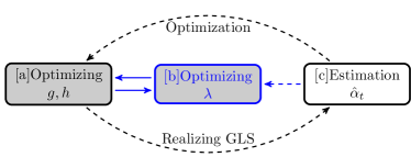
Figure 2: Illustration of proposed algorithm (WADN) and relation with other scenarios. WADN consists three components: [a] learning embedding function $g$ and classifier $h$; [b] source aggregation through properly estimating $\bm{\lambda}$; [c] label distribution ratio ($\hat{\alpha}_{t}$) estimator. (1) If target labels are available, then WADN only requires [a,b] without gradually estimating $\hat{\alpha}_{t}$ (dashed arrows). (2) In the unsupervised scenarios, if we only have one source, WADN only contains [a,c] and recovers the single DA problem with label proportion shift, which can be solved under specific assumptions such as GLS (Li et al., 2019b; Combes et al., 2020) or (Wu et al., 2019). (3) If there are multiple sources in the unsupervised DA, WADN gradually selects the related sources through interacting with other algorithmic components. (shown in blue).

4.1 Training Rules

Based on Theorem 2, given a fixed label ratio $\hat{\alpha}_{t}$ and fixed $\bm{\lambda}$, the goal is to find a representation function $g:\mathcal{X}\to\mathcal{Z}$ and a hypothesis function $h:\mathcal{Z}\times\mathcal{Y}\to\mathbb{R}$ such that:

$$\begin{split}\min_{g,h}&\sum_{t}\bm{\lambda}[t]\hat{R}^{\hat{\alpha}_{t}}_{\mathcal{S}_{t}}(h,g)\\ &+C_{0}\sum_{t}\bm{\lambda}[t]\mathbb{E}_{y\sim\hat{\mathcal{T}}(y)}W_{1}(\hat{\mathcal{S}}_{t}(z|Y=y)\|\hat{\mathcal{T}}(z|Y=y))\end{split}$$

Explicit Conditional Loss

One can explicitly solve the conditional optimal transport problem with $g$ and $h$ for a given $Y=y$. However, due to the high computational complexity in solving $T\times|\mathcal{Y}|$ optimal transport problems, the original form is practically intractable. To address this, we can approximate the conditional distribution on latent space $Z$ as Gaussian distribution with identical Covariance matrix such that $\hat{\mathcal{S}}_{t}(z|Y=y)\approx\mathcal{N}(\mathbf{C}^{y}_{t},\mathbf{\Sigma})$ and $\hat{\mathcal{T}}(z|Y=y)\approx\mathcal{N}(\mathbf{C}^{y},\mathbf{\Sigma})$. Then we have $W_{1}(\hat{\mathcal{S}}_{t}(z|Y=y)\|\hat{\mathcal{T}}(z|Y=y))\leq\|\mathbf{C}^{y}_{t}-\mathbf{C}^{y}\|_{2}$. Intuitively, the approximation term is equivalent to the well known feature mean matching (Sugiyama & Kawanabe, 2012), which computes the feature centroid of each class (on the latent space $Z$) and aligns them by minimizing their $L_{2}$ distance.

Implicit Conditional Loss

Apart from approximation, we can derive a dual term for facilitating the computation, which is equivalent to the re-weighted Wasserstein adversarial loss by the label-distribution ratio.

Lemma 1.

The weighted conditional Wasserstein distance can be implicitly expressed as:

$$\begin{split}&\sum_{t}\bm{\lambda}[t]\mathbb{E}_{y\sim\mathcal{T}(y)}W_{1}(\mathcal{S}_{t}(z|Y=y)\|\mathcal{T}(z|Y=y))\\ &=\max_{d_{1},\cdots,d_{T}}\sum_{t}\bm{\lambda}[t][\mathbb{E}_{z\sim\mathcal{S}_{t}(z)}\bar{\alpha}_{t}(z)d_{t}(z)-\mathbb{E}_{z\sim\mathcal{T}(z)}d_{t}(z)],\end{split}$$

where $\bar{\alpha}_{t}(z)=\mathbf{1}_{\{(z,y)\sim\mathcal{S}_{t}\}}\alpha_{t}(Y=y)$, and $d_{1},\dots,d_{T}:\mathcal{Z}\to R_{+}$ are the $1$-Lipschitz domain discriminators (Ganin et al., 2016).

Lemma 1 reveals that one can train $T$ domain discriminators with weighted Wasserstein adversarial loss. When the source target distributions are identical, this loss recovers the conventional Wasserstein adversarial loss (Arjovsky et al., 2017). In practice, we adopt a hybrid approach by linearly combining the explicit and implicit matching, in which empirical results show its effectiveness.

Estimation $\hat{\alpha}$

When the target labels are available, $\hat{\alpha}_{t}$ can be directly estimated from the data with $\hat{\alpha}_{t}(y)=\hat{\mathcal{T}}(y)/\hat{\mathcal{S}}(y)$ and $\hat{\alpha}_{t}\to\alpha_{t}$ can be proved from asymptotic statistics. As for the unsupervised scenarios, we will discuss in Sec. 5.1.

4.2 Estimation Relation Coefficient $\bm{\lambda}$

Inspired by Theorem 1, given a fixed $\hat{\alpha}_{t}$ and $(g,h)$, we estimate $\bm{\lambda}$ through optimizing the derived upper bound.

$$\begin{split}\min_{\bm{\lambda}}\quad&\sum_{t}\bm{\lambda}[t]\hat{R}^{\hat{\alpha}_{t}}_{\mathcal{S}_{t}}(h,g)+C_{1}\sqrt{\sum_{t=1}^{T}\frac{\bm{\lambda}^{2}[t]}{\beta_{t}}}\\ &+C_{0}\sum_{t}\bm{\lambda}[t]\mathbb{E}_{y\sim\hat{\mathcal{T}}(y)}W_{1}(\hat{\mathcal{T}}(z|Y=y)\|\hat{\mathcal{S}}(z|Y=y))\\ \text{s.t}&\quad\forall t,\bm{\lambda}[t]\geq 0,\sum_{t=1}^{T}\bm{\lambda}[t]=1\end{split}$$

In practice, $\hat{R}^{\hat{\alpha}_{t}}_{\mathcal{S}_{t}}(h,g)$ is the weighted empirical prediction loss and $\mathbb{E}_{y\sim\hat{\mathcal{T}}(y)}W_{1}(\hat{\mathcal{T}}(z|Y=y)\|\hat{\mathcal{S}}(z|Y=y))$ is approximated by the dynamic form of critic function from Lemma 1. Then, solving $\bm{\lambda}$ can be viewed as a standard convex optimization problem with linear constraints, which can be effectively resolved through standard convex optimizer.

5 Extension to Unsupervised Scenarios

In this section, we extend WADN to the unsupervised multi-source DA, which is known as unsolvable if semantic conditional distribution ($\mathcal{S}_{t}(x|y)\neq\mathcal{T}(x|y)$) and label distribution ($\mathcal{S}_{t}(y)\neq\mathcal{T}(y)$) are simultaneously different and no specific conditions are considered (Ben-David et al., 2010b; Johansson et al., 2019).

In algorithm WADN, this challenging turns to properly estimate conditional Wasserstein distance and label distribution ratio $\hat{\alpha}_{t}(y)$ to help estimate $\bm{\lambda}$. According to Lemma 1, estimating the conditional Wasserstein distance can be viewed as $\hat{\alpha}_{t}$-weighted adversarial loss, thus if we can correctly estimate label distribution ratio such that $\hat{\alpha}_{t}\to\alpha_{t}$, then we can properly compute the conditional Wasserstein-distance through the adversarial term.

Therefore, the problem turns to properly estimate the label distribution ratio. To this end, we assume the problem satisfies Generalized Label Shift (GLS) condition (Combes et al., 2020), which has been theoretically justified and empirically evaluated in the single source unsupervised DA. The GLS condition states that in unsupervised DA, there exists an optimal embedding function $g^{\star}\in\mathcal{G}$ that can ultimately achieve $\mathcal{S}_{t}(z|y)=\mathcal{T}(z|y)$ on the latent space. (Combes et al., 2020) further pointed out that the clustering assumption (Chapelle & Zien, 2005) on $\mathcal{Z}$ is one sufficient condition to reach GLS, which is feasible for many practical applications.

Based on the achievability condition of GLS, the techniques of (Lipton et al., 2018; Garg et al., 2020) can be adopted to gradually estimate $\hat{\alpha}_{t}$ during learning the embedding function. Following this spirit, we add an distribution ratio estimator for $\{\hat{\alpha}_{t}\}_{t=1}^{T}$, shown in Sec. 5.1.

5.1 Estimation $\hat{\alpha}_{t}$

Unsupervised DA

We denote $\bar{\mathcal{S}}_{t}(y)$, $\bar{\mathcal{T}}(y)$ as the predicted $t$-source/target label distribution through the hypothesis $h$, and also define $C_{\hat{\mathcal{S}}_{t}}[y,k]=\hat{\mathcal{S}}_{t}[\text{argmax}_{y^{\prime}}h(z,y^{\prime})=y,Y=k]$ is the $t$-source prediction confusion matrix. According to the GLS condition, we have $\bar{\mathcal{T}}(y)=\bar{\mathcal{T}}_{\hat{\alpha}_{t}}(y)$, with $\bar{\mathcal{T}}_{\hat{\alpha}_{t}}(Y=y)=\sum_{k=1}^{\mathcal{Y}}C_{\hat{\mathcal{S}}_{t}}[y,k]\hat{\alpha}_{t}(k)$ the constructed target prediction distribution from the $t$-source information. (See Appendix for justification). Then we can estimate $\hat{\alpha}_{t}$ through matching these two distributions by minimizing $D_{\text{KL}}(\bar{\mathcal{T}}(y)\|\bar{\mathcal{T}}_{\hat{\alpha}_{t}}(y))$, which is equivalent to solve the following convex optimization:

$$\begin{split}&\min_{\hat{\alpha}_{t}}\quad-\sum_{y=1}^{|\mathcal{Y}|}\bar{\mathcal{T}}(y)\log(\sum_{k=1}^{|\mathcal{Y}|}C_{\hat{\mathcal{S}}_{t}}[y,k]\hat{\alpha}_{t}(k))\\ &\text{s.t}\quad\forall y\in\mathcal{Y},\hat{\alpha}_{t}(y)\geq 0,\quad\sum_{y=1}^{|\mathcal{Y}|}\hat{\alpha}_{t}(y)\hat{\mathcal{S}}_{t}(y)=1\end{split}$$ (1)

Unsupervised Partial DA

If we have $\text{supp}(\mathcal{T}(y))\subseteq\text{supp}(\mathcal{S}_{t}(y))$, ${\alpha}_{t}$ will be sparse due to the non-overlapped classes. Thus, we impose such prior knowledge by adding a regularizer $\|\hat{\alpha}_{t}\|_{1}$ to the objective of Eq. (1) to induce the sparsity in $\hat{\alpha}_{t}$.

In training the neural network, the non-overlapped classes will be automatically assigned with a small or zero $\hat{\alpha}_{t}$, then $(g,h)$ will be less affected by the classes with small $\hat{\alpha}_{t}$.

Algorithm 1 WADN (unsupervised scenario, one epoch)

0:  Label ratio $\hat{\alpha}_{t}$ and task relation $\bm{\lambda}$. Feature Learner $g$, Classifier $h$, statistic critic function $d_{1},\dots,d_{T}$, class centroid for source $\mathbf{C}_{t}^{y}$ and target $\mathbf{C}^{y}$.($t=1,\dots,T$)

1:  $\triangleright$ DNN Parameter Training Stage (fixed $\alpha_{t}$ and $\bm{\lambda}$) $\triangleleft$

2:  for mini-batch of samples $(\mathbf{x}_{\mathcal{S}_{1}},\mathbf{y}_{\mathcal{S}_{1}})\sim\hat{\mathcal{S}}_{1}$, $\dots$, $(\mathbf{x}_{\mathcal{S}_{T}},\mathbf{y}_{\mathcal{S}_{T}})\sim\hat{\mathcal{S}}_{T}$, $(\mathbf{x}_{\mathcal{T}})\sim\hat{\mathcal{T}}$  do

3:     Target predicted-label $\bar{\mathbf{y}}_{\mathcal{T}}=\text{argmax}_{y}h(g(\mathbf{x}_{\mathcal{T}}),y)$

4:     Compute unnormalized source confusion matrix on current batch $C_{\hat{\mathcal{S}}_{t}}[y,k]$.

5:     Compute feature centroid for source $C_{t}^{y}$ and target $C^{y}$ on current batch; Use moving average to update source and target class centroid $\mathbf{C}_{t}^{y}$ and $\mathbf{C}^{y}$.

6:     Updating $g,h,d_{1},\dots,d_{T}$, by optimizing:

$$\min_{g,h}\max_{d_{1},\dots,d_{T}}\underbrace{\sum\mathop{}_{\mkern-3.0mut}\bm{\lambda}[t]\hat{R}^{\hat{\alpha}_{t}}_{\mathcal{S}_{t}}(h,g)}_{\text{Classification Loss}}\\ +\epsilon C_{0}\underbrace{\sum\mathop{}_{\mkern-3.0mut}\bm{\lambda}[t]\mathbb{E}_{y\sim\bar{\mathcal{T}}(y)}\|\mathbf{C}_{t}^{y}-\mathbf{C}^{y}\|_{2}}_{\text{Explicit Conditional Loss}}\\ +(1-\epsilon)C_{0}\underbrace{\sum\mathop{}_{\mkern-3.0mut}\bm{\lambda}[t][\mathbb{E}_{z\sim\hat{\mathcal{S}}_{t}(z)}\bar{\alpha}_{t}(z)d(z)-\mathbb{E}_{z\sim\hat{\mathcal{T}}(z)}d(z)]}_{\text{Implicit Conditional Loss}}$$

7:  end for

8:  $\triangleright$ Estimation $\hat{\alpha}_{t}$ and $\bm{\lambda}$ $\triangleleft$

9:  Compute normalized source confusion matrix; Solve $\{\hat{\alpha}_{t}\}_{t=1}^{T}$ w.r.t. current training epoch through Sec.5.1 ; Update global $\hat{\alpha}_{t}$ through moving average.

10:  Solve $\bm{\lambda}$ through Sec.4.2 w.r.t. current training epoch; Update global $\bm{\lambda}$ through moving average.

Table 1: Unsupervised DA: Accuracy $(\%)$ on Source-Shifted Amazon Review (Left) and Digits (Right).

Target	Books	DVD	Electronics	Kitchen	Average
Source	68.15±1.37	69.51±0.74	82.09±0.88	75.30±1.29	73.81
DANN	65.59±1.35	67.23±0.71	80.49±1.11	74.71±1.53	72.00
MDAN	68.77±2.31	67.81±2.46	80.96±0.77	75.67±1.96	73.30
MDMN	70.56±1.05	69.64±0.73	82.71±0.71	77.05±0.78	74.99
M3SDA	69.09±1.26	68.67±1.37	81.34±0.66	76.10±1.47	73.79
DARN	71.21±1.16	68.68±1.12	81.51±0.81	77.71±1.09	74.78
WADN	73.72±0.63	79.64±0.34	84.64±0.48	83.73±0.50	80.43

Target	MNIST	SVHN	SYNTH	USPS	Average
Source	84.93±1.50	67.14±1.40	78.11±1.31	86.02±1.12	79.05
DANN	86.99±1.53	69.56±2.26	78.73±1.30	86.81±1.74	80.52
MDAN	87.86±2.24	69.13±1.56	79.77±1.69	86.50±1.59	80.81
MDMN	87.31±1.88	69.84±1.59	80.27±0.88	86.61±1.41	81.00
M3SDA	87.22±1.70	68.89±1.93	80.01±1.77	86.39±1.68	80.87
DARN	86.98±1.29	68.59±1.79	80.68±0.61	86.85±1.78	80.78
WADN	89.07±0.72	71.66±0.77	82.06±0.89	90.07±1.10	83.22

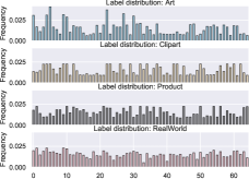
Figure 3: Label distribution on Office-Home Dataset

Table 2: Unsupervised DA: Accuracy $(\%)$ on Office-Home

Target	Art	Clipart	Product	Real-World	Average
Source	49.25±0.60	46.89±0.61	66.54±1.72	73.64±0.91	59.08
DANN	50.32±0.32	50.11±1.16	68.18±1.27	73.71±1.63	60.58
MDAN	67.93±0.36	66.61±1.32	79.24±1.52	81.82±0.65	73.90
MDMN	68.38±0.58	67.42±0.53	82.49±0.56	83.32±1.93	75.28
M3SDA	63.77±1.07	62.30±0.44	75.85±1.24	79.92±0.60	70.46
DARN	69.89±0.42	68.61±0.50	83.37±0.62	84.29±0.46	76.54
WADN	73.78±0.43	70.18±0.54	86.32±0.38	87.28±0.87	79.39

5.2 Algorithm implementation and discussion

We give an algorithmic description of Fig. 2, shown in Algorithm 1. The high-level protocol is to iteratively optimizes the neural-network parameters to gradually realize GLS condition with $g\to g^{\star}$ and dynamically update $\bm{\lambda}$, $\hat{\alpha}_{t}$ to better estimate conditional distance and aggregate the sources. The GLS assumes the achievability of existing an optimal $g^{\star}$. Our iterative algorithm can achieve a stationary solution but due to the highly non-convexity of deep network, converging to the global optimal does not necessarily guarantee.

Concretely, we update the $\hat{\alpha}_{t}$ and $\bm{\lambda}$ on the fly through a moving averaging strategy. Within one training epoch over the mini-batches, we fix the $\hat{\alpha}_{t}$ and $\bm{\lambda}$ and optimize the network parameters $g,h$. Then at each training epoch, we re-estimate the $\hat{\alpha}_{t}$ and $\bm{\lambda}$ by using the proposed estimator. When computing the explicit conditional loss, we empirically adopt the target pseudo-label. The implicit and explicit trade-off coefficient is set as $\epsilon=0.5$. As for optimization $\bm{\lambda}$ and $\alpha_{t}$, it is a standard convex optimization problem and we use package CVXPY.

As for WADN with limited target label, we do not require label distribution ratio component and directly compute $\hat{\alpha}_{t}$.

6 Experiments

In this section, we compare the proposed approaches with several baselines on the popular tasks. For all the scenarios, the following multi-source DA baselines are evaluated: (I) Source method applied only labelled source data to train the model. (II) DANN (Ganin et al., 2016). We follow the protocol of (Wen et al., 2020) to merge all the source dataset as a global source domain. (III) MDAN (Zhao et al., 2018); (IV) MDMN (Li et al., 2018b); (V) M³SDA (Peng et al., 2019) adopted maximizing classifier discrepancy (Saito et al., 2018) and (VI) DARN (Wen et al., 2020). For the multi-source with limited target label and partial unsupervised multi-source DA, we additionally add specific baselines. All the baselines are re-implemented in the same network structure for fair comparisons. The detailed network structures, hyper-parameter settings, training details are delegated in Appendix.

We evaluate the performance on three different datasets: (1) Amazon Review. (Blitzer et al., 2007) It contains four domains (Books, DVD, Electronics, and Kitchen) with positive and negative product reviews. We follow the common data pre-processing strategies as (Chen et al., 2012) to form a $5000$-dimensional bag-of-words feature. Note that the label distribution in the original dataset is uniform. To show the benefits of the proposed approach, we create a label distribution drifted task by randomly dropping $50\%$ negative reviews of all the sources while keeping the target identical. (2) Digits. It consists four digits recognition datasets including MNIST, USPS (Hull, 1994), SVHN (Netzer et al., 2011) and Synth (Ganin et al., 2016). We also create a label distribution drift for the sources by randomly dropping $50\%$ samples on digits 5-9 and keep target identical. (3) Office-Home Dataset (Venkateswara et al., 2017). It contains 65 classes for four different domains: Art, Clipart, Product and Real-World. We used the ResNet50 (He et al., 2016) pretrained from the ImageNet in PyTorch as the base network for feature learning and put a MLP for the classification. The label distributions in these four domains are different and we did not manually create a label drift, shown in Fig. 3.

Table 3: Multi-Source DA with Limited Target Label: Accuracy $(\%)$ on Source-Shifted Amazon Review (Left) and Digits (Right).

Target	Books	DVD	Electronics	Kitchen	Average
Source + Tar	72.59±1.89	73.02±1.84	81.59±1.58	77.03±1.73	76.06
DANN	67.35±2.28	66.33±2.42	78.03±1.72	74.31±1.71	71.50
MDAN	68.70±2.99	69.30±2.21	78.78±2.21	74.07±1.89	72.71
MDMN	69.19±2.09	68.71±2.39	81.88±1.46	78.51±1.91	74.57
M3SDA	69.28±1.78	67.40±0.46	76.28±0.81	76.50±1.19	72.36
DARN	68.57±1.35	68.77±1.81	80.19±1.66	77.51±1.20	73.76
RLUS	71.83±1.71	69.64±2.39	81.98±1.04	78.69±1.15	75.54
MME	69.66±0.58	71.36±0.96	78.88±1.51	76.64±1.73	74.14
WADN	74.83±0.84	75.05±0.62	84.23±0.58	81.53±0.90	78.91

Target	MNIST	SVHN	SYNTH	USPS	Average
Source + Tar	79.63±1.74	56.48±1.90	69.64±1.38	86.29±1.56	73.01
DANN	86.77±1.30	69.13±1.09	78.82±1.35	86.54±1.03	80.32
MDAN	86.93±1.05	68.25±1.53	79.80±1.17	86.23±1.41	80.30
MDMN	77.59±1.36	69.62±1.26	78.93±1.64	87.26±1.13	78.35
M3SDA	85.88±2.06	68.84±1.05	76.29±0.95	87.15±1.10	79.54
DARN	86.58±1.46	68.86±1.30	80.47±0.67	86.80±0.89	80.68
RLUS	87.61±1.08	70.50±0.94	79.52±1.30	86.70±1.13	81.08
MME	87.24±0.95	65.20±1.35	80.31±0.60	87.88±0.76	80.16
WADN	88.32±1.17	70.64±1.02	81.53±1.11	90.53±0.71	82.75

(a) Visualization of $\bm{\lambda}$

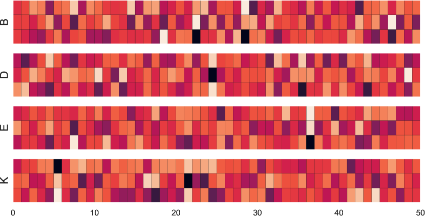
(b) DARN (Wen et al., 2020)

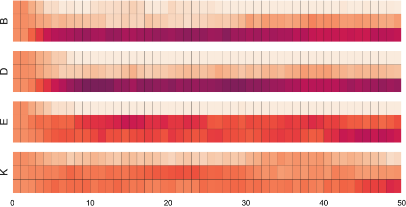
(c) WADN

Figure 4: Understanding Aggregation Principles in Unsupervised DA. (a) Visualization of $\bm{\lambda}$ on digits datset, each row corresponds to a target domain, which indicates a non-uniform and non-symmetric task relations. (b,c) The evolution of $\bm{\lambda}$ with three sources of Amazon dataset (B=Books, D=DVD, E=Electronics, K=Kitchen) during the training epoch. We compare with a recent principle approach DARN, which uses $\mathbb{P}(x)$ to measure the similarity and dynamically update the $\bm{\lambda}$. The results verifies the limitation of DARN under changing label distributions with relative unstable results.

6.1 Unsupervised Multi-Source DA

In the unsupervised multi-source DA, we evaluate the proposed approach on all three datasets. We use a similar hyper-parameter selection strategy as in DANN (Ganin et al., 2016). All reported results are averaged from five runs. The detailed experimental settings are illustrated in Appendix. The empirical results are illustrated in Tab. 1 and 2. Since we did not change the target label distribution throughout the whole experiment, we still report the target accuracy as the metric. We report the means and standard deviations for each approach. The best approaches based on a two-sided Wilcoxon signed-rank test (significance level $p=0.05$) are shown in bold.

The empirical results reveal a significantly better performance ($\approx 2\%-6\%$) on different benchmarks. For understanding the aggregation principles of WADN, we visualize the task relations in digits (Fig. 4(a)) with demonstrating a non-uniform $\bm{\lambda}$, which highlights the importance of properly choosing the most related source rather than simply merging all the data. For example, when the target domain is SVHN, WADN mainly leverages the information from SYNTH, since they are more semantically similar, and MNIST does not help too much for SVHN, which is also observed by (Ganin et al., 2016). Besides, Fig. 4(b) visualizes the evolution of $\bm{\lambda}$ between WADN and recent principled approach DARN (Wen et al., 2020), which utilized the $\mathbb{P}(x)$ information and dynamic updating to find the similar domains. Compared with WADN, $\bm{\lambda}$ in DARN is unstable during updating under drifted label distribution.

Besides, we conduct the ablation study through evaluating the performance under different levels of source label shift in Amazon Review dataset (Fig. 5(a)). The results show strong practical benefits for WADN in the larger label shift. The additional analysis and results can be found in Appendix.

6.2 Multi-Source DA with Limited Target Labels

We adopt Amazon Review and Digits in the multi-source DA with limited target samples, which have been widely used. In the experiments, we still use shifted sources. We randomly sample only $10\%$ labeled samples (w.r.t. target dataset in unsupervised DA) as training set and the rest $90\%$ samples as the unseen target test set. We adopt the same hyper-parameters and training strategies with unsupervised DA. We specifically add two recent baselines RLUS (Konstantinov & Lampert, 2019) and MME (Saito et al., 2019), which also considered DA with the labeled target domain.

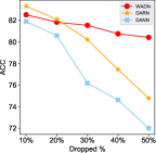
(a)

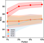
(b)

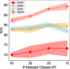
(c)

Figure 5: Ablation study on different scenarios. (a) Unsupervised DA with Amazon Review dataset. Accuracy under different levels of label shifted sources (higher dropping rate means larger label drift). The results are reported on the average of all the domains, see the results for each domain in Appendix. (b) Multi-Source DA with limited target label in digits task with target USPS. The performance (mean $\pm$ std) of WADN is consistently better under different target samples (smaller portion indicates fewer target samples). (C) Partial Multi-source DA in office-home dataset with target domain Product. Performance (mean $\pm$ std) of different number of selected classes on the target, where WADN shows a consistent better performance under different selected sub-classes.

The results are reported in Tab. 3, which also indicates strong empirical improvement. Interestingly, on the Amazon review dataset, the previous aggregation approach RLUS is unable to select the related source when label distribution varies. To show the effectiveness of WADN, we test various portions of labelled samples ($1\%\sim 10\%$) on the target. The results in Fig. 5(b) on USPS dataset show consistently better than the baseline, even in the few target samples scenarios such as $1-3\%$.

Table 4: Unsupervised Multi-Source Partial DA: Accuracy $(\%)$ on Office-Home (#Source: 65, #Target: 35)

Target	Art	Clipart	Product	Real-World	Average
Source	50.56±1.42	49.79±1.14	68.10±1.33	78.24±0.76	61.67
DANN	53.86±2.23	52.71±2.20	71.25±2.44	76.92±1.21	63.69
MDAN	67.56±1.39	65.38±1.30	81.49±1.92	83.44±1.01	74.47
MDMN	68.13±1.08	65.27±1.93	81.33±1.29	84.00±0.64	74.68
M3SDA	65.10±1.97	61.80±1.99	76.19±2.44	79.14±1.51	70.56
DARN	71.53±0.63	69.31±1.08	82.87±1.56	84.76±0.57	77.12
PADA	74.37±0.84	69.64±0.80	83.45±1.13	85.64±0.39	78.28
WADN	80.06±0.93	75.90±1.06	89.55±0.72	90.40±0.39	83.98

6.3 Partial Unsupervised Multi-Source DA

In this scenario, we adopt the Office-Home dataset to evaluate our approach, as it contains large (65) classes. We do not change the source domains and we randomly choose 35 classes from the target. We evaluate all the baselines on the same selected classes and repeat 5 times. All reported results are averaged from 3 different sub-class selections (15 runs in total), shown in Tab. 4. We additionally compare PADA (Cao et al., 2018) approach by merging all sources and use one-to-one partial DA algorithm. We adopt the same hyper-parameters and training strategies in unsupervised DA scenario.

The reported results are also significantly better than the current multi-source DA or one-to-one partial DA approach, which again emphasizes the benefits of WADN: properly selecting the related sources by using semantic information.

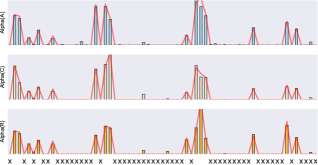
Figure 6: Analysis on Partial DA of target Product. We select 15 classes and visualize estimated $\hat{\alpha}_{t}$ (the bar plot). The ”X” along the x-axis represents the index of dropped 50 classes. The red curves are the true label distribution ratio. See Appendix for additional results and analysis.

Besides, we change the number of selected classes (Fig 5(c)), the proposed WADN still indicates consistent better results by a large margin, which indicates the importance of considering $\hat{\alpha}_{t}$ and $\bm{\lambda}$. In contrast, DANN shows unstable results on average in less selected classes. Beside, WADN shows a good estimation of the label distribution ratio (Fig 6) and has correctly detected the non-overlapping classes, which verifies the effectiveness of the label-distribution estimator and indicates its good explainability.

7 Conclusion

In this paper, we proposed a novel algorithm WADN for multi-source domain adaptation problem under different label proportions. WADN differs from previous approaches in two key prospects: a better source aggregation approach when label distributions change; a unified empirical framework for three popular DA scenarios. We evaluated the proposed method by extensive experiments and showed its strong empirical results.

Appendix A Additional Related Work

Additional Multi-source DA Theory

has been investigated in the previous literature. In the unsupervised DA, (Ben-David et al., 2010a; Zhao et al., 2018; Peng et al., 2019) adopted $\mathcal{H}$-divergence of marginal distribution $\mathcal{D}(x)$ to estimate the domain relations.(Li et al., 2018b) also applied Wasserstein distance of $\mathcal{D}(x)$ to estimate pair-wise domain distance. (Mansour et al., 2009b; Wen et al., 2020) used the Discrepancy distance to derive a tighter theoretical bound. The motivated practice from the aforementioned method used the feature information to learn the task relations, with the general following forms:

$$R_{\mathcal{T}}(h)\leq\sum_{t}\bm{\lambda}[t]R_{\mathcal{S}}(h)+\sum_{t}\bm{\lambda}[t]d(\mathcal{S}_{t}(x),\mathcal{T}(x))+\beta$$

However, as we stated in the paper, $d(\mathcal{S}_{t}(x),\mathcal{T}(x))$ is not a proper to measure the task’s relations. Besides, (Hoffman et al., 2018a) used Rényi divergence that requires $\text{supp}(\mathcal{T}(x))\subseteq\text{supp}(\mathcal{S}(x))$, which generally does not hold in the complicated real-world applications. (Konstantinov & Lampert, 2019; Mansour et al., 2020) adopted $\mathcal{Y}$-discrepancy (Mohri & Medina, 2012) to measure the joint distribution similarity. However, $\mathcal{Y}$ discrepancy is practically difficult to estimate from the data and we empirically show it is difficult to handle the target-shifted sources.

Multi-source DA Practice

has been proposed from various prospective. The key idea is to estimate the importance of different sources and then select the most related ones, to mitigate the influence of negative transfer. In the multi-source unsupervised DA, (Sankaranarayanan et al., 2018; Balaji et al., 2019; Pei et al., 2018; Zhao et al., 2019; Zhu et al., 2019; Zhao et al., 2020, 2019; Stojanov et al., 2019; Li et al., 2019b; Wang et al., 2019c; Lin et al., 2020) proposed different practical strategies in the classification, regression and semantic segmentation problems. In the presence of available labels on the target domain, (Hoffman et al., 2012; Tan et al., 2013; Wei et al., 2017; Yao & Doretto, 2010; Konstantinov & Lampert, 2019) used generalized linear model to learn the target. (Christodoulidis et al., 2016; Li et al., 2019a; Chen et al., 2019) focused on deep learning approaches and (Lee et al., 2019) proposed an ad-hoc strategy to combine to sources in the few-shot target domains. In contrast, these ideas are generally data-driven approaches and do not propose a principled practice to understand the source combination and understand task relations.

Label-Partial Unsupervised DA

Label-Partial can be viewed as a special case of the target-shifted DA. Most existing works focus on one-to-one partial DA (Zhang et al., 2018; Chen et al., 2020; Bucci et al., 2019; Cao et al., 2019) by adopting the re-weighting training approach without a principled understanding. In our paper, we first analyzed this common practice and adopt the label distribution ratio as its weights, which provides a principled approach to detect the non-overlapped classes in the representation learning.

A.1 Other scenarios related to Multi-Source DA

Domain Generalization

The domain generalization (DG) resembles multi-source transfer but aims at different goals. A common setting in DG is to learn multiple source but directly predict on the unseen target domain. The conventional DG approaches generally learn a distribution invariant features (Balaji et al., 2018; Saenko et al., 2010; Motiian et al., 2017; Ilse et al., 2019) or conditional distribution invariant features (Li et al., 2018c; Akuzawa et al., 2019). However, our theoretical results reveal that in the presence of label shift (i.e $\alpha_{t}(y)\neq 1$) and outlier tasks then learning conditional or marginal invariant features can not guarantee a small target risk. Our theoretical result enables a formal understanding about the inherent difficulty in DG problems.

Multi-Task Learning

The goal of multi-task learning (Zhang & Yang, 2017) aims to improve the prediction performance of all the tasks. In our paper, we aim at controlling the prediction risk of a specified target domain. We also notice some practical techniques are common such as the shared parameter (Zhang & Yeung, 2012), shared representation (Ruder, 2017), etc.

Appendix B Additional Figures

We additionally visualize the label distributions in our experiments.

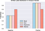
(a) Amazon

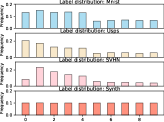
(b) Digits

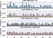
(c) Office-Home

Figure 7: Label distribution visualization. (a) One example in Amazon Review dataset with sources: Book, Dvd, Electronic and target: Kitchen. We randomly drop $50\%$ of the negative reviews in all the sources while keeping target label distribution unchanged. (b) One example in Digits dataset with Sources: MNIST, USPS, SVHN and Target Synth. We randomly drop $50\%$ data on digits 5-9 in all sources while keeping target label distribution unchanged. (c) Office-Home dataset. The original label distribution is non-uniform. See Appendix L for details.

Appendix C Notation Tables

Table 5: Table of Notations

$R_{\mathcal{D}}(h)=\mathbb{E}_{(x,y)\sim\mathcal{D}}\ell(h(x,y))$		Expected Risk on distribution $\mathcal{D}$ w.r.t. hypothesis $h$
$\hat{R}_{\mathcal{D}}(h)=\frac{1}{N}\sum_{i=1}^{N}\ell(h(x_{i},y_{i}))$		Empirical Risk on observed data $\{(x_{i},y_{i})\}_{i=1}^{N}$ that are i.i.d. sampled from $\mathcal{D}$.
$\alpha$ and $\hat{\alpha}_{t}$		True and empirical label distribution ratio $\alpha(y)=\mathcal{T}(y)/\mathcal{S}(y)$
$\hat{R}^{\alpha}_{\mathcal{S}}(h)=\frac{1}{N}\sum_{i=1}^{N}\alpha(y_{i})\ell(h(x_{i},y_{i}))$		Empirical Weighted Risk on observed data $\{(x_{i},y_{i})\}_{i=1}^{N}$.
$\mathcal{S}(z|y)=\int_{x}g(z|x)S(x|Y=y)dx$		Conditional distribution w.r.t. latent variable $Z$ that induced by feature learning function $g$.
$W_{1}(\mathcal{S}_{t}(z|y)\|\mathcal{T}(z|y))$		Conditional Wasserstein distance on the latent space $Z$

Appendix D Proof of Theorem 1

Proof idea

Theorem 1 consists three steps in the proof:

Lemma 2.

If the prediction loss is assumed as $L$-Lipschitz and the hypothesis is $K$-Lipschitz w.r.t. the feature $x$ (given the same label), i.e. for $\forall Y=y$, $\|h(x_{1},y)-h(x_{2},y)\|_{2}\leq K\|x_{1}-x_{2}\|_{2}$. Then the target risk can be upper bounded by:

$$R_{\mathcal{T}}(h)\leq\sum_{t}\bm{\lambda}[t]R^{\alpha_{t}}_{\mathcal{S}}(h)+LK\sum_{t}\bm{\lambda}[t]\mathbb{E}_{y\sim\mathcal{T}(y)}W_{1}(\mathcal{T}(x|Y=y)\|\mathcal{S}(x|Y=y))$$ (2)

Proof.

The target risk can be expressed as:

$$R_{\mathcal{T}}(h(x,y))=\mathbb{E}_{(x,y)\sim\mathcal{T}}\ell(h(x,y))=\mathbb{E}_{y\sim\mathcal{T}(y)}\mathbb{E}_{x\sim\mathcal{T}(x|y)}\ell(h(x,y))$$

By denoting $\alpha(y)=\frac{\mathcal{T}(y)}{\mathcal{S}(y)}$, then we have:

$$\mathbb{E}_{y\sim\mathcal{T}(y)}\mathbb{E}_{y\sim\mathcal{T}(x|y)}\ell(h(x,y))=\mathbb{E}_{y\sim\mathcal{S}(y)}\alpha(y)\mathbb{E}_{x\sim\mathcal{T}(x|y)}\ell(h(x,y))$$

Then we aim to upper bound $\mathbb{E}_{x\sim\mathcal{T}(x|y)}\ell(h(x,y))$. For any fixed $y$,

$$\mathbb{E}_{x\sim\mathcal{T}(x|y)}\ell(h(x,y))-\mathbb{E}_{x\sim\mathcal{S}(x|y)}\ell(h(x,y))\leq|\int_{x\in\mathcal{X}}\ell(h(x,y))d(\mathcal{T}(x|y)-\mathcal{S}(x|y))|$$

Then according to the Kantorovich-Rubinstein duality, for any distribution coupling $\gamma\in\Pi(\mathcal{T}(x|y),\mathcal{S}(x|y))$, then we have:

$$\begin{split}&=\inf_{\gamma}|\int_{\mathcal{X}\times\mathcal{X}}\ell(h(x_{p},y))-\ell(h(x_{q},y))d\gamma(x_{p},x_{q})|\\ &\leq\inf_{\gamma}\int_{\mathcal{X}\times\mathcal{X}}|\ell(h(x_{p},y))-\ell(h(x_{q},y))|d\gamma(x_{p},x_{q})\\ &\leq L\inf_{\gamma}\int_{\mathcal{X}\times\mathcal{X}}|h(x_{p},y))-h(x_{q},y)|d\gamma(x_{p},x_{q})\\ &\leq LK\inf_{\gamma}\int_{\mathcal{X}\times\mathcal{X}}\|x_{p}-x_{q}\|_{2}d\gamma(x_{p},x_{q})\\ &=LKW_{1}(\mathcal{T}(x|Y=y)\|\mathcal{S}(x|Y=y))\end{split}$$

The first inequality is obvious; and the second inequality comes from the assumption that $\ell$ is $L$-Lipschitz; the third inequality comes from the hypothesis is $K$-Lipschitz w.r.t. the feature $x$ (given the same label), i.e. for $\forall Y=y$, $\|h(x_{1},y)-h(x_{2},y)\|_{2}\leq K\|x_{1}-x_{2}\|_{2}$.

Then we have:

$$\begin{split}R_{\mathcal{T}}(h)&\leq\mathbb{E}_{y\sim\mathcal{S}(y)}\alpha(y)[\mathbb{E}_{x\sim\mathcal{S}(x|y)}\ell(h(x,y))+LKW_{1}(\mathcal{T}(x|y)\|\mathcal{S}(x|y))]\\ &=\mathbb{E}_{(x,y)\sim\mathcal{S}}\alpha(y)\ell(h(x,y))+LK\mathbb{E}_{y\sim\mathcal{T}(y)}W_{1}(\mathcal{T}(x|Y=y)\|\mathcal{S}(x|Y=y))\\ &=R^{\alpha}_{\mathcal{S}}(h)+LK\mathbb{E}_{y\sim\mathcal{T}(y)}W_{1}(\mathcal{T}(x|Y=y)\|\mathcal{S}(x|Y=y))\end{split}$$

Supposing each source $\mathcal{S}_{t}$ we assign the weight $\bm{\lambda}[t]$ and label distribution ratio $\alpha_{t}(y)=\frac{\mathcal{T}(y)}{\mathcal{S}_{t}(y)}$, then by combining this $T$ source target pair, we have:

$$R_{\mathcal{T}}(h)\leq\sum_{t}\bm{\lambda}[t]R^{\alpha_{t}}_{\mathcal{S}_{t}}(h)+LK\sum_{t}\bm{\lambda}[t]\mathbb{E}_{y\sim\mathcal{T}(y)}W_{1}(\mathcal{T}(x|Y=y)\|\mathcal{S}_{t}(x|Y=y))$$

∎

Then we will prove Theorem 1 from this result, we will derive the non-asymptotic bound, estimated from the finite sample observations. Supposing the empirical label ratio value is $\hat{\alpha}_{t}$, then for any simplex $\bm{\lambda}$ we can prove the high-probability bound.

D.1 Bounding the empirical and expected prediction risk

Proof.

We first bound the first term, which can be upper bounded as:

$$\sup_{h}|\sum_{t}\bm{\lambda}[t]R^{\alpha_{t}}_{\mathcal{S}_{t}}(h)-\sum_{t}\bm{\lambda}[t]\hat{R}^{\hat{\alpha}_{t}}_{\mathcal{S}_{t}}(h)|\leq\underbrace{\sup_{h}|\sum_{t}\bm{\lambda}[t]R^{\alpha_{t}}_{\mathcal{S}_{t}}(h)-\sum_{t}\bm{\lambda}[t]\hat{R}^{\alpha_{t}}_{\mathcal{S}_{t}}(h)|}_{(\textup{I})}+\underbrace{\sup_{h}|\sum_{t}\bm{\lambda}[t]\hat{R}^{\alpha_{t}}_{\mathcal{S}_{t}}(h)-\sum_{t}\bm{\lambda}[t]\hat{R}^{\hat{\alpha}_{t}}_{\mathcal{S}_{t}}(h)|}_{(\textup{II})}$$

Bounding term $(\textup{I})$

According to the McDiarmid inequality, each item changes at most $|\frac{2\bm{\lambda}[t]\alpha_{t}(y)\ell}{N_{\mathcal{S}_{t}}}|$. Then we have:

$$P\left((\textup{I})-\mathbb{E}(\textup{I})\geq t\right)\leq\exp(\frac{-2t^{2}}{\sum_{t=1}^{T}\frac{4}{\beta_{t}N}\bm{\lambda}^{2}[t]\alpha_{t}(y)^{2}\ell^{2}})=\delta$$

By substituting $\delta$, at high probability $1-\delta$ we have:

$$(\textup{I})\leq\mathbb{E}(\textup{I})+L_{\max}d^{\sup}_{\infty}\sqrt{\sum_{t=1}^{T}\frac{\bm{\lambda}[t]^{2}}{\beta_{t}}}\sqrt{\frac{\log(1/\delta)}{2N}}$$

Where $L_{\max}=\sup_{h\in\mathcal{H}}\ell(h)$ and $N=\sum_{t=1}^{T}N_{\mathcal{S}_{t}}$ the total source observations and $\beta_{t}=\frac{N_{\mathcal{S}_{t}}}{N}$ the frequency ratio of each source. And $d_{\infty}^{\sup}=\max_{t=1,\dots,T}d_{\infty}(\mathcal{T}(y)\|\mathcal{S}(y))=\max_{t=1,\dots,T}\max_{y\in[1,\mathcal{Y}]}\alpha_{t}(y)$, the maximum true label shift value (constant).

Bounding $\mathbb{E}\sup(\textup{I})$, the expectation term can be upper bounded as the form of Rademacher Complexity:

$$\begin{split}\mathbb{E}(\textup{I})&\leq 2\mathbb{E}_{\sigma}\mathbb{E}_{\hat{\mathcal{S}}_{1}^{T}}\sup_{h}\sum_{t=1}^{T}\bm{\lambda}[t]\sum_{(x_{t},y_{t})\in\hat{\mathcal{S}_{t}}}\frac{1}{TN}\left(\alpha_{t}(y)\ell(h(x_{t},y_{t})\right)\\ &\leq 2\sum_{t}\bm{\lambda}[t]\mathbb{E}_{\sigma}\mathbb{E}_{\hat{\mathcal{S}}_{1}^{T}}\sup_{h}\sum_{(x_{t},y_{t})\in\hat{\mathcal{S}_{t}}}\frac{1}{TN}\left(\alpha_{t}(y)\ell(h(x_{t},y_{t})\right)\\ &\leq 2\sup_{t}\mathbb{E}_{\sigma}\mathbb{E}_{\hat{\mathcal{S}}_{t}}\sup_{h}\sum_{(x_{t},y_{t})\in\hat{\mathcal{S}_{t}}}\frac{1}{TN}\left[\alpha_{t}(y)\ell(h(x_{t},y_{t}))\right]\\ &=\sup_{t}2\mathcal{R}_{t}(\ell,\mathcal{H})=2\bar{R}(\ell,\mathcal{H})\end{split}$$

Where $\bar{R}(\ell,\mathcal{H})=\sup_{t}\mathcal{R}_{t}(\ell,\mathcal{H})=\sup_{t}\sup_{h\sim\mathcal{H}}\mathbb{E}_{\hat{\mathcal{S}}_{t},\sigma}\sum_{(x_{t},y_{t})\in\hat{\mathcal{S}_{t}}}\frac{1}{TN}\left[\alpha_{t}(y)\ell(h(x_{t},y_{t}))\right]$, represents the Rademacher complexity w.r.t. the prediction loss $\ell$, hypothesis $h$ and true label distribution ratio $\alpha_{t}$.

Therefore with high probability $1-\delta$, we have:

$$\sup_{h}|\sum_{t}\bm{\lambda}[t]R^{\alpha_{t}}_{\mathcal{S}}(h)-\sum_{t}\bm{\lambda}[t]\hat{R}^{\alpha_{t}}_{\mathcal{S}}(h)|\leq\bar{\mathcal{R}}(\ell,h)+L_{\max}d^{\sup}_{\infty}\sqrt{\sum_{t=1}^{T}\frac{\bm{\lambda}[t]^{2}}{\beta_{t}}}\sqrt{\frac{\log(1/\delta)}{2N}}$$

Bounding Term $(\textup{II})$

For all the hypothesis $h$, we have:

$$\begin{split}|\sum_{t}\bm{\lambda}[t]\hat{R}^{\alpha_{t}}_{\mathcal{S}_{t}}(h)-\sum_{t}\bm{\lambda}[t]\hat{R}^{\hat{\alpha}_{t}}_{\mathcal{S}_{t}}(h)|&=|\sum_{t}\bm{\lambda}[t]\frac{1}{N_{\mathcal{S}_{t}}}\sum_{i}^{N_{\mathcal{S}_{t}}}(\alpha(y(i))-\hat{\alpha}(y(i)))\ell(h)|\\ &=\sum_{t}\bm{\lambda}[t]\frac{1}{N_{\mathcal{S}_{t}}}|\sum_{y}^{|\mathcal{Y}|}(\alpha(Y=y)-\hat{\alpha}(Y=y))\bar{\ell}(Y=y)|\end{split}$$

Where $\bar{\ell}(Y=y)=\sum_{i}^{N_{\mathcal{S}_{t}}}\ell(h(x_{i},y_{i}=y))$, represents the cumulative error, conditioned on a given label $Y=y$. According to the Holder inequality, we have:

$$\begin{split}\sum_{t}\bm{\lambda}[t]\frac{1}{N_{\mathcal{S}_{t}}}|\sum_{y}^{|\mathcal{Y}|}(\alpha_{t}(Y=y)-\hat{\alpha}_{t}(Y=y))\bar{\ell}(Y=y)|&\leq\sum_{t}\bm{\lambda}[t]\frac{1}{N_{\mathcal{S}_{t}}}\|\alpha_{t}-\hat{\alpha}_{t}\|_{2}\|\bar{\ell}(Y=y)\|_{2}\\ &\leq L_{\max}\sum_{t}\bm{\lambda}[t]\|\alpha_{t}-\hat{\alpha}_{t}\|_{2}\\ &\leq L_{\max}\sup_{t}\|\alpha_{t}-\hat{\alpha}_{t}\|_{2}\end{split}$$

Therefore, $\forall h\in\mathcal{H}$, with high probability $1-\delta$ we have:

$$\sum_{t}\bm{\lambda}[t]R^{\alpha_{t}}_{\mathcal{S}}(h)\leq\sum_{t}\bm{\lambda}[t]\hat{R}^{\hat{\alpha}_{t}}_{\mathcal{S}}(h)+2\bar{\mathcal{R}}(\ell,h)+L_{\max}d^{\sup}_{\infty}\sqrt{\sum_{t=1}^{T}\frac{\bm{\lambda}[t]^{2}}{\beta_{t}}}\sqrt{\frac{\log(1/\delta)}{2N}}+L_{\max}\sup_{t}\|\alpha_{t}-\hat{\alpha}_{t}\|_{2}$$

D.2 Bounding empirical Wasserstein Distance

Then we need to derive the sample complexity of the empirical and true distributions, which can be decomposed as the following two parts. For any $t$, we have:

$$\begin{split}&\mathbb{E}_{y\sim\mathcal{T}(y)}W_{1}(\mathcal{T}(x|Y=y)\|\mathcal{S}_{t}(x|Y=y))-\mathbb{E}_{y\sim\hat{\mathcal{T}}(y)}W_{1}(\hat{\mathcal{T}}(x|Y=y)\|\hat{\mathcal{S}_{t}}(x|Y=y))\\ &\underbrace{\leq\mathbb{E}_{y\sim\mathcal{T}(y)}W_{1}(\mathcal{T}(x|Y=y)\|\mathcal{S}_{t}(x|Y=y))-\mathbb{E}_{y\sim\mathcal{T}(y)}W_{1}(\hat{\mathcal{T}}(x|Y=y)\|\hat{\mathcal{S}_{t}}(x|Y=y))}_{(\textup{I})}\\ &+\underbrace{\mathbb{E}_{y\sim\mathcal{T}(y)}W_{1}(\hat{\mathcal{T}}(x|Y=y)\|\hat{\mathcal{S}_{t}}(x|Y=y))-\mathbb{E}_{y\sim\hat{\mathcal{T}}(y)}W_{1}(\hat{\mathcal{T}}(x|Y=y)\|\hat{\mathcal{S}_{t}}(x|Y=y))}_{(\textup{II})}\end{split}$$

Bounding $(\textup{I})$

We have:

$$\begin{split}&\mathbb{E}_{y\sim\mathcal{T}(y)}W_{1}(\mathcal{T}(x|Y=y)\|\mathcal{S}_{t}(x|Y=y))-\mathbb{E}_{y\sim\mathcal{T}(y)}W_{1}(\hat{\mathcal{T}}(x|Y=y)\|\hat{\mathcal{S}_{t}}(x|Y=y))\\ &=\sum_{y}\mathcal{T}(y)\left(W_{1}(\mathcal{T}(x|Y=y)\|\mathcal{S}_{t}(x|Y=y))-W_{1}(\hat{\mathcal{T}}(x|Y=y)\|\hat{\mathcal{S}_{t}}(x|Y=y)\right)\\ &\leq|\sum_{y}\mathcal{T}(y)|\sup_{y}\left(W_{1}(\mathcal{T}(x|Y=y)\|\mathcal{S}_{t}(x|Y=y))-W_{1}(\hat{\mathcal{T}}(x|Y=y)\|\hat{\mathcal{S}_{t}}(x|Y=y)\right)\\ &=\sup_{y}\left(W_{1}(\mathcal{T}(x|Y=y)\|\mathcal{S}_{t}(x|Y=y))-W_{1}(\hat{\mathcal{T}}(x|Y=y)\|\hat{\mathcal{S}_{t}}(x|Y=y)\right)\\ &\leq\sup_{y}~{}[W_{1}(\mathcal{S}_{t}(x|Y=y)\|\hat{\mathcal{S}_{t}}(x|Y=y))+W_{1}(\hat{\mathcal{S}_{t}}(x|Y=y)\|\hat{\mathcal{T}}(x|Y=y))\\ &+W_{1}(\hat{\mathcal{T}}(x|Y=y)\|\mathcal{T}(x|Y=y))-W_{1}(\hat{\mathcal{T}}(x|Y=y)\|\hat{\mathcal{S}_{t}}(x|Y=y))]\\ &=\sup_{y}W_{1}(\mathcal{S}_{t}(x|Y=y)\|\hat{\mathcal{S}_{t}}(x|Y=y))+W_{1}(\hat{\mathcal{T}}(x|Y=y)\|\mathcal{T}(x|Y=y))\end{split}$$

The first inequality holds because of the Holder inequality. As for the second inequality, we use the triangle inequality of Wasserstein distance. $W_{1}(P\|Q)\leq W_{1}(P\|P_{1})+W_{1}(P_{1}\|P_{2})+W_{1}(P_{2}\|Q)$.

According to the convergence behavior of Wasserstein distance (Weed et al., 2019), with high probability $\geq 1-2\delta$ we have:

$$W_{1}(\mathcal{S}_{t}(x|Y=y)\|\hat{\mathcal{S}_{t}}(x|Y=y))+W_{1}(\hat{\mathcal{T}}(x|Y=y)\|\mathcal{T}(x|Y=y))\leq\kappa(\delta,N^{y}_{\mathcal{S}_{t}},N^{y}_{\mathcal{T}})$$

Where $k(\delta,N^{y}_{\mathcal{S}_{t}},N^{y}_{\mathcal{T}})=C_{t,y}(N^{y}_{\mathcal{S}_{t}})^{-s_{t,y}}+C_{y}(N^{y}_{\mathcal{T}})^{-s_{y}}+\sqrt{\frac{1}{2}\log(\frac{2}{\delta})}(\sqrt{\frac{1}{N^{y}_{\mathcal{S}_{t}}}}+\sqrt{\frac{1}{N_{t}^{y}}})$, where $N^{y}_{\mathcal{S}_{t}}$ is the number of $Y=y$ in source $t$ and $N^{y}_{\mathcal{T}}$ is the number of $Y=y$ in target distribution. $C_{t,y}$, $C_{y}$ $s_{t,y}>2$, $s_{y}>2$ are positive constant in the concentration inequality. This indicates the convergence behavior between empirical and true Wasserstein distance.

If we adopt the union bound (over all the labels) by setting $\delta\leftarrow\delta/|\mathcal{Y}|$, then with high probability $\geq 1-2\delta$, we have:

$$\sup_{y}W_{1}(\mathcal{S}(x|Y=y)\|\hat{\mathcal{S}}(x|Y=y))+W_{1}(\hat{\mathcal{T}}(x|Y=y)\|\mathcal{T}(x|Y=y))\leq\kappa(\delta,N^{y}_{\mathcal{S}_{t}},N^{y}_{\mathcal{T}})$$

where $\kappa(\delta,N^{y}_{\mathcal{S}_{t}},N^{y}_{\mathcal{T}})=C_{t,y}(N^{y}_{\mathcal{S}_{t}})^{-s_{t,y}}+C_{y}(N^{y}_{\mathcal{T}})^{-s_{y}}+\sqrt{\frac{1}{2}\log(\frac{2|\mathcal{Y}|}{\delta})}(\sqrt{\frac{1}{N^{y}_{\mathcal{S}_{t}}}}+\sqrt{\frac{1}{N^{y}_{\mathcal{T}}}})$

Again by adopting the union bound (over all the tasks) by setting $\delta\leftarrow\delta/T$, with high probability $\geq 1-2\delta$, we have:

$$\sum_{t}\bm{\lambda}[t]\mathbb{E}_{y\sim\mathcal{T}(y)}W_{1}(\mathcal{T}(x|Y=y)\|\mathcal{S}(x|Y=y))-\sum_{t}\bm{\lambda}[t]\mathbb{E}_{y\sim\mathcal{T}(y)}W_{1}(\hat{\mathcal{T}}(x|Y=y)\|\hat{\mathcal{S}}(x|Y=y))\leq\sup_{t}\kappa(\delta,N^{y}_{\mathcal{S}_{t}},N^{y}_{\mathcal{T}})$$

Where $\kappa(\delta,N^{y}_{\mathcal{S}_{t}},N^{y}_{\mathcal{T}})=C_{t,y}(N^{y}_{\mathcal{S}_{t}})^{-s_{t,y}}+C_{y}(N^{y}_{\mathcal{T}})^{-s_{y}}+\sqrt{\frac{1}{2}\log(\frac{2T|\mathcal{Y}|}{\delta})}(\sqrt{\frac{1}{N^{y}_{\mathcal{S}_{t}}}}+\sqrt{\frac{1}{N^{y}_{\mathcal{T}}}})$.

Bounding $(\textup{II})$

We can bound the second term:

$$\begin{split}&\mathbb{E}_{y\sim\mathcal{T}(y)}W_{1}(\hat{\mathcal{T}}(x|Y=y)\|\hat{\mathcal{S}_{t}}(x|Y=y))-\mathbb{E}_{y\sim\hat{\mathcal{T}}(y)}W_{1}(\hat{\mathcal{T}}(x|Y=y)\|\hat{\mathcal{S}_{t}}(x|Y=y))\\ &\leq\sup_{y}W_{1}(\hat{\mathcal{T}}(x|Y=y)\|\hat{\mathcal{S}_{t}}(x|Y=y))|\sum_{y}\mathcal{T}(y)-\hat{\mathcal{T}}(y)|\\ &\leq C^{t}_{\text{max}}|\sum_{y}\mathcal{T}(y)-\hat{\mathcal{T}}(y)|\end{split}$$

Where $C^{t}_{\text{max}}=\sup_{y}W_{1}(\hat{\mathcal{T}}(x|Y=y)\|\hat{\mathcal{S}}(x|Y=y))$ is a positive and bounded constant. Then we need to bound $|\sum_{y}\mathcal{T}(y)-\hat{\mathcal{T}}(y)|$, by adopting MicDiarmid’s inequality, we have at high probability $1-\delta$:

$$|\sum_{y}\mathcal{T}(y)-\hat{\mathcal{T}}(y)| \leq\mathbb{E}_{\hat{\mathcal{T}}}|\sum_{y}\mathcal{T}(y)-\hat{\mathcal{T}}(y)|+\sqrt{\frac{\log(1/\delta)}{2N_{\mathcal{T}}}}$$

$$=2\mathbb{E}_{\sigma}\mathbb{E}_{\hat{\mathcal{T}}}\sum_{y}\sigma\hat{\mathcal{T}}(y)+\sqrt{\frac{\log(1/\delta)}{2N_{\mathcal{T}}}}$$

Then we bound $\mathbb{E}_{\sigma}\mathbb{E}_{\hat{\mathcal{T}}}\sum_{y}\sigma\hat{\mathcal{T}}(y)$. We use the properties of Rademacher complexity [Lemma 26.11, (Shalev-Shwartz & Ben-David, 2014)] and notice that $\hat{\mathcal{T}}(y)$ is a probability simplex, then we have:

$$\mathbb{E}_{\sigma}\mathbb{E}_{\hat{\mathcal{T}}}\sum_{y}\sigma\hat{\mathcal{T}}(y)\leq\sqrt{\frac{2\log(2|\mathcal{Y}|)}{N_{\mathcal{T}}}}$$

Then we have $|\sum_{y}\mathcal{T}(y)-\hat{\mathcal{T}}(y)|\leq\sqrt{\frac{2\log(2|\mathcal{Y}|)}{N_{\mathcal{T}}}}+\sqrt{\frac{\log(1/\delta)}{2N_{\mathcal{T}}}}$

Then using the union bound and denoting $\delta\leftarrow\delta/T$, with high probability $\geq 1-\delta$ and for any simplex $\bm{\lambda}$, we have:

$$\begin{split}\sum_{t}\bm{\lambda}[t]\mathbb{E}_{y\sim\mathcal{T}(y)}W_{1}(\hat{\mathcal{T}}(x|Y=y)\|\hat{\mathcal{S}_{t}}(x|Y=y))&\leq\sum_{t}\bm{\lambda}[t]\mathbb{E}_{y\sim\hat{\mathcal{T}}(y)}W_{1}(\hat{\mathcal{T}}(x|Y=y)\|\hat{\mathcal{S}_{t}}(x|Y=y))\\ &C_{\max}(\sqrt{\frac{2\log(2|\mathcal{Y}|)}{N_{\mathcal{T}}}}+\sqrt{\frac{\log(T/\delta)}{2N_{\mathcal{T}}}})\end{split}$$

where $C_{\max}=\sup_{t}C^{t}_{\max}$.

Combining together, we can derive the PAC-Learning bound, which is estimated from the finite samples (with high probability $1-4\delta$):

$$\begin{split}R_{\mathcal{T}}(h)&\leq\sum_{t}\bm{\lambda}_{t}\hat{R}^{\hat{\alpha}_{t}}_{\mathcal{S}_{t}}(h)+LH\sum_{t}\bm{\lambda}_{t}\mathbb{E}_{y\sim\hat{\mathcal{T}}(y)}W_{1}(\hat{\mathcal{T}}(x|Y=y)\|\hat{\mathcal{S}}(x|Y=y))+L_{\max}d^{\sup}_{\infty}\sqrt{\sum_{t=1}^{T}\frac{\bm{\lambda}_{t}^{2}}{\beta_{t}}}\sqrt{\frac{\log(1/\delta)}{2N}}\\ &+2\bar{\mathcal{R}}(\ell,h)+L_{\max}\sup_{t}\|\alpha_{t}-\hat{\alpha}_{t}\|_{2}+\sup_{t}\kappa(\delta,N^{y}_{\mathcal{S}_{t}},N^{y}_{\mathcal{T}})+C_{\max}(\sqrt{\frac{2\log(2|\mathcal{Y}|)}{N_{\mathcal{T}}}}+\sqrt{\frac{\log(T/\delta)}{2N_{\mathcal{T}}}})\end{split}$$

Then we denote $\text{Comp}(N_{\mathcal{S}_{1}},\dots,N_{\mathcal{T}},\delta)=2\bar{\mathcal{R}}(\ell,h)+\sup_{t}\kappa(\delta,N^{y}_{\mathcal{S}_{t}},N^{y}_{\mathcal{T}})+C_{\max}(\sqrt{\frac{2\log(2|\mathcal{Y}|)}{N_{\mathcal{T}}}}+\sqrt{\frac{\log(T/\delta)}{2N_{\mathcal{T}}}})$ as the convergence rate function that decreases with larger $N_{\mathcal{S}_{1}},\dots,N_{\mathcal{T}}$. Bedsides, $\bar{\mathcal{R}}(\ell,h)=\sup_{t}\mathcal{R}_{t}(\ell,\mathcal{H})$ is the re-weighted Rademacher complexity. Given a fixed hypothesis with finite VC dimension , it can be proved $\bar{\mathcal{R}}(\ell,h)=\min_{N_{\mathcal{S}_{1}},\dots,N_{\mathcal{S}_{T}}}\mathcal{O}(\sqrt{\frac{1}{N_{\mathcal{S}_{t}}}})$ i.e (Shalev-Shwartz & Ben-David, 2014). ∎

Appendix E Proof of Theorem 2

We first recall the stochastic feature representation $g$ such that $g:\mathcal{X}\to\mathcal{Z}$ and scoring hypothesis h $h:\mathcal{Z}\times\mathcal{Y}\to\mathbb{R}$ and the prediction loss $\ell$ with $\ell:\mathbb{R}\to\mathbb{R}$.

Proof.

The marginal distribution and conditional distribution w.r.t. latent variable $Z$ that are induced by $g$, which can be reformulated as:

$$\mathcal{S}(z)=\int_{x}g(z|x)\mathcal{S}(x)dx\quad\quad\mathcal{S}(z|y)=\int_{x}g(z|x)\mathcal{S}(x|Y=y)dx$$

In the multi-class classification problem, we additionally define the following distributions:

$$\mu^{k}(z)=\mathcal{S}(Y=k,z)=\mathcal{S}(Y=k)\mathcal{S}(z|Y=k)$$

$$\pi^{k}(z)=\mathcal{T}(Y=k,z)=\mathcal{T}(Y=k)\mathcal{T}(z|Y=k)$$

Based on (Nguyen et al., 2009) and $g(z|x)$ is a stochastic representation learning function, the loss conditioned a fixed point $(x,y)$ w.r.t. $h$ and $g$ is $\mathbb{E}_{z\sim g(z|x)}\ell(h(z,y))$. Then taking the expectation over the $\mathcal{S}(x,y)$ we have:

$$\begin{split}R_{\mathcal{S}}(h,g)&=\mathbb{E}_{(x,y)\sim\mathcal{S}(x,y)}\mathbb{E}_{z\sim g(z|x)}\ell(h(z,y))\\ &=\sum_{k=1}^{|\mathcal{Y}|}\mathcal{S}(y=k)\int_{x}\mathcal{S}(x|Y=k)\int_{z}g(z|x)\ell(h(z,y=k))dzdx\\ &=\sum_{k=1}^{|\mathcal{Y}|}\mathcal{S}(y=k)\int_{z}[\int_{x}\mathcal{S}(x|Y=k)g(z|x)dx]\ell(h(z,y=k))dz\\ &=\sum_{k=1}^{|\mathcal{Y}|}\mathcal{S}(y=k)\int_{z}\mathcal{S}(z|Y=k)\ell(h(z,y=k))dz\\ &=\sum_{k=1}^{|\mathcal{Y}|}\int_{z}\mathcal{S}(z,Y=k)\ell(h(z,y=k))dz\\ &=\sum_{k=1}^{|\mathcal{Y}|}\int_{z}\mu^{k}(z)\ell(h(z,y=k))dz\end{split}$$

Intuitively, the expected loss w.r.t. the joint distribution $\mathcal{S}$ can be decomposed as the expected loss on the label distribution $\mathcal{S}(y)$ (weighted by the labels) and conditional distribution $\mathcal{S}(\cdot|y)$ (real valued conditional loss).

Then the expected risk on the $\mathcal{S}$ and $\mathcal{T}$ can be expressed as:

$$R_{\mathcal{S}}(h,g)=\sum_{k=1}^{|\mathcal{Y}|}\int_{z}\ell(h(z,y=k))\mu^{k}(z)dz$$

$$R_{\mathcal{T}}(h,g)=\sum_{k=1}^{|\mathcal{Y}|}\int_{z}\ell(h(z,y=k))\pi^{k}(z)dz$$

By denoting $\alpha(y)=\frac{\mathcal{T}(y)}{\mathcal{S}(y)}$, we have the $\alpha$-weighted loss:

$$\begin{split}R^{\alpha}_{\mathcal{S}}(h,g)=&\mathcal{T}(Y=1)\int_{z}\ell(h(z,y=1))\mathcal{S}(z|Y=1)+\mathcal{T}(Y=2)\int_{z}\ell(h(z,y=2))\mathcal{S}(z|Y=2)\\ &+\dots+\mathcal{T}(Y=k)\int_{z}\ell(h(z,y=k))\mathcal{S}(z|Y=k)dz\end{split}$$

Then we have:

$$\begin{split}R_{\mathcal{T}}(h,g)-R^{\alpha}_{\mathcal{S}}(h,g)&\leq\sum_{k}\mathcal{T}(Y=k)\int_{z}\ell(h(z,y=k))d|\mathcal{S}(z|Y=k)-\mathcal{T}(z|Y=k)|\\ \end{split}$$

Under the same assumption, we have the loss function $\ell(h(z,Y=k))$ is KL-Lipschitz w.r.t. the cost $\|\cdot\|_{2}$ (given a fixed $k$). Therefore by adopting the same proof strategy (Kantorovich-Rubinstein duality) in Lemma 2, we have

$$\begin{split}&\leq KL\mathcal{T}(Y=1)W_{1}(\mathcal{S}(z|Y=1)\|\mathcal{T}(z|Y=1))+\dots+KL\mathcal{T}(Y=k)W_{1}(\mathcal{S}(z|Y=k)\|\mathcal{T}(z|Y=k))\\ &=KL\mathbb{E}_{y\sim\mathcal{T}(y)}W_{1}(\mathcal{S}(z|Y=y)\|\mathcal{T}(z|Y=y))\end{split}$$

Therefore, we have:

$$R_{\mathcal{T}}(h,g)\leq R^{\alpha}_{\mathcal{S}}(h,g)+LK\mathbb{E}_{y\sim\mathcal{T}(y)}W_{1}(\mathcal{S}(z|Y=y)\|\mathcal{T}(z|Y=y))$$

Based on the aforementioned result, we have $\forall t=1,\dots,T$ and denote $\mathcal{S}=\mathcal{S}_{t}$ and $\alpha(y)=\alpha_{t}(y)=\mathcal{T}(y)/\mathcal{S}_{t}(y)$:

$$\bm{\lambda}[t]R_{\mathcal{T}}(h,g)\leq\bm{\lambda}[t]R^{\alpha_{t}}_{\mathcal{S}_{t}}(h,g)+LK\bm{\lambda}[t]\mathbb{E}_{y\sim\mathcal{T}(y)}W_{1}(\mathcal{S}_{t}(z|Y=y)\|\mathcal{T}(z|Y=y))$$

Summing over $t=1,\dots,T$, we have:

$$R_{\mathcal{T}}(h,g)\leq\sum_{t=1}^{T}\bm{\lambda}[t]R^{\alpha_{t}}_{\mathcal{S}_{t}}(h,g)+LK\sum_{t=1}^{T}\bm{\lambda}[t]\mathbb{E}_{y\sim\mathcal{T}(y)}W_{1}(\mathcal{S}_{t}(z|Y=y)\|\mathcal{T}(z|Y=y))$$

∎

Appendix F Approximation $W_{1}$ distance

According to Jensen inequality, we have

$$W_{1}(\hat{\mathcal{S}}_{t}(z|Y=y)\|\hat{\mathcal{T}}(z|Y=y))\leq\sqrt{[W_{2}(\hat{\mathcal{S}}_{t}(z|Y=y)\|\hat{\mathcal{T}}(z|Y=y))]^{2}}$$

Supposing $\hat{\mathcal{S}}_{t}(z|Y=y)\approx\mathcal{N}(\mathbf{C}^{y}_{t},\mathbf{\Sigma})$ and $\hat{\mathcal{T}}(z|Y=y)\approx\mathcal{N}(\mathbf{C}^{y},\mathbf{\Sigma})$, then we have:

$$[W_{2}(\hat{\mathcal{S}}_{t}(z|Y=y)\|\hat{\mathcal{T}}(z|Y=y)]^{2}=\|\mathbf{C}^{y}_{t}-\mathbf{C}^{y}\|_{2}^{2}+\text{Trace}(2\mathbf{\Sigma}-2(\mathbf{\Sigma}\mathbf{\Sigma})^{1/2})=\|\mathbf{C}^{y}_{t}-\mathbf{C}^{y}\|_{2}^{2}$$

We would like to point out that assuming the identical covariance matrix is more computationally efficient during the matching. This is advantageous and reasonable in the deep learning regime: we adopted the mini-batch (ranging from 20-128) for the neural network parameter optimization, in each mini-batch the samples of each class are small, then we compute the empirical covariance/variance matrix will be surely biased to the ground truth variance and induce a much higher complexity to optimize. By the contrary, the empirical mean is unbiased and computationally efficient, we can simply use the moving the moving average to efficiently update the estimated mean value (with a unbiased estimator). The empirical results verify the effectiveness of this idea.

Appendix G Proof of Lemma 1

For each source $\mathcal{S}_{t}$, by introducing the duality of Wasserstein-1 distance, for $y\in\mathcal{Y}$, we have:

$$\begin{split}W_{1}(\mathcal{S}_{t}(z|y)\|\mathcal{T}(z|y))&=\sup_{\|d\|_{L}\leq 1}\mathbb{E}_{z\sim\mathcal{S}_{t}(z|y)}d(z)-\mathbb{E}_{z\sim\mathcal{T}(z|y)}d(z)\\ &=\sup_{\|d\|_{L}\leq 1}\sum_{z}\mathcal{S}_{t}(z|y)d(z)-\sum_{z}\mathcal{T}(z|y)d(z)\\ &=\frac{1}{\mathcal{T}(y)}\sup_{\|d\|_{L}\leq 1}\frac{\mathcal{T}(y)}{\mathcal{S}_{t}(y)}\sum_{z}\mathcal{S}_{t}(z,y)d(z)-\sum_{z}\mathcal{T}(z,y)d(z)\end{split}$$

Then by defining $\bar{\alpha}_{t}(z)=\mathbf{1}_{\{(z,y)\sim\mathcal{S}_{t}\}}\frac{\mathcal{T}(Y=y)}{\mathcal{S}_{t}(Y=y)}=\mathbf{1}_{\{(z,y)\sim\mathcal{S}_{t}\}}\alpha_{t}(Y=y)$, we can see for each pair observation $(z,y)$ sampled from the same distribution, then $\bar{\alpha}_{t}(Z=z)=\alpha_{t}(Y=y)$. Then we have:

$$\begin{split}\sum_{y}\mathcal{T}(y)W_{1}(\mathcal{S}_{t}(z|y)\|\mathcal{T}(z|y))&=\sum_{y}\sup_{\|d\|_{L}\leq 1}\{\sum_{z}\alpha_{t}(y)\mathcal{S}_{t}(z,y)d(z)-\sum_{z}\mathcal{T}(z,y)d(z)\}\\ &=\sup_{\|d\|_{L}\leq 1}\sum_{z}\bar{\alpha}_{t}(z)\mathcal{S}_{t}(z)d(z)-\sum_{z}\mathcal{T}(z)d(z)\\ &=\sup_{\|d\|_{L}\leq 1}\mathbb{E}_{z\sim\mathcal{S}_{t}(z)}\bar{\alpha}_{t}(z)d(z)-\mathbb{E}_{z\sim\mathcal{T}(z)}d(z)\end{split}$$

We propose a simple example to understand $\bar{\alpha}_{t}$: supposing three samples in $\mathcal{S}_{t}=\{(z_{1},Y=1),(z_{2},Y=1),(z_{3},Y=0)\}$ then $\bar{\alpha}_{t}(z_{1})=\bar{\alpha}_{t}(z_{2})=\alpha_{t}(1)$ and $\bar{\alpha}_{t}(z_{3})=\alpha_{t}(0)$. Therefore, the conditional term is equivalent to the label-weighted Wasserstein adversarial learning. We plug in each source domain as weight $\bm{\lambda}[t]$ and domain discriminator as $d_{t}$, we finally have Lemma 1.

Appendix H Derive the label distribution ratio Loss

In GLS, we have $\mathcal{T}(z|y)\approx\mathcal{S}_{t}(z|y)$, $\forall t$, then we suppose the predicted target distribution as $\bar{\mathcal{T}}(y)$. By simplifying the notation, we define $f(z)=\text{argmax}_{y}h(z,y)$ the most possible prediction label output, then we have:

$$\bar{\mathcal{T}}(y) =\sum_{k=1}^{\mathcal{Y}}\mathcal{T}(f(z)=y|Y=k)\mathcal{T}(Y=k)=\sum_{k=1}^{\mathcal{Y}}\mathcal{S}_{t}(f(z)=y|Y=k)\mathcal{T}(Y=k)$$

$$=\sum_{i=1}^{\mathcal{Y}}\mathcal{S}_{t}(f(z)=y,Y=k)\alpha_{t}(k)=\bar{\mathcal{T}}_{\alpha_{t}}(y)$$

The first equality comes from the definition of target label prediction distribution, $\bar{\mathcal{T}}(y)=\mathbb{E}_{\mathcal{T}(z)}\mathbf{1}\{f(z)=y\}=\mathcal{T}(f(z)=y)=\sum_{k=1}^{\mathcal{Y}}\mathcal{T}(f(z)=y,Y=k)=\sum_{k=1}^{\mathcal{Y}}\mathcal{T}(f(z)=y|Y=k)\mathcal{T}(Y=k)$.

The second equality $\mathcal{T}(f(z)=y|Y=k)=\mathcal{S}_{t}(f(z)=y|Y=k)$ holds since $\forall t$, $\mathcal{T}(z|y)\approx\mathcal{S}_{t}(z|y)$, then for the shared hypothesis $f$, we have $\mathcal{T}(f(z)=y|Y=k)=\mathcal{S}_{t}(f(z)=y|Y=k)$.

The term $\mathcal{S}_{t}(f(z)=y,Y=k)$ is the (expected) source prediction confusion matrix, and we denote its empirical (observed) version as $\hat{\mathcal{S}}_{t}(f(z)=y,Y=k)$.

Based on this idea, in practice we want to find a $\hat{\alpha}_{t}$ to match the two predicted distribution $\bar{\mathcal{T}}$ and $\bar{\mathcal{T}}_{\hat{\alpha}_{t}}$. If we adopt the KL-divergence as the metric, we have:

$$\min_{\hat{\alpha}_{t}}D_{\text{KL}}(\bar{\mathcal{T}}\|\bar{\mathcal{T}}_{\hat{\alpha}_{t}}) =\min_{\hat{\alpha}_{t}}\mathbb{E}_{y\sim\bar{\mathcal{T}}}\log(\frac{\bar{\mathcal{T}}(y)}{\bar{\mathcal{T}}_{\hat{\alpha}_{t}}(y)})=\min_{\hat{\alpha}_{t}}-\mathbb{E}_{y\sim\bar{\mathcal{T}}}\log(\bar{\mathcal{T}}_{\hat{\alpha}_{t}}(y))$$

$$=\min_{\hat{\alpha}_{t}}-\sum_{y}\bar{\mathcal{T}}(y)\log(\sum_{k=1}^{\mathcal{Y}}\mathcal{S}_{t}(f(z)=y,Y=k)\hat{\alpha}_{t}(k))$$

We should notice the nature constraints of label ratio: $\{\hat{\alpha}_{t}(y)\geq 0,\sum_{y}\hat{\alpha}_{t}(y)\hat{\mathcal{S}}_{t}(y)=1\}$. Based on this principle, we proposed the optimization problem to estimate each label ratio. We adopt its empirical counterpart, the empirical confusion matrix $C_{\hat{\mathcal{S}}_{t}}[y,k]=\hat{\mathcal{S}}_{t}[f(z)=y,Y=k]$, then the optimization loss can be expressed as:

$$\min_{\hat{\alpha}_{t}} \quad\quad-\sum_{y=1}^{|\mathcal{Y}|}\bar{\mathcal{T}}(y)\log(\sum_{k=1}^{|\mathcal{Y}|}C_{\hat{\mathcal{S}}_{t}}[y,k]\hat{\alpha}_{t}(k))$$

$$\text{s.t.}\quad\forall y\in\mathcal{Y},\hat{\alpha}_{t}(y)\geq 0,\quad\sum_{y}\hat{\alpha}_{t}(y)\hat{\mathcal{S}}_{t}(y)=1$$

Appendix I Label Partial Multi-source unsupervised DA

The key difference between multi-conventional and partial unsupervised DA is the estimation step of $\hat{\alpha}_{t}$. In fact, we only add a sparse constraint for estimating each $\hat{\alpha}_{t}$:

$$\begin{split}\min_{\hat{\alpha}_{t}}&\quad\quad-\sum_{y=1}^{|\mathcal{Y}|}\bar{\mathcal{T}}(y)\log(\sum_{k=1}^{|\mathcal{Y}|}C_{\hat{\mathcal{S}}_{t}}[y,k]\hat{\alpha}_{t}(k))+C_{2}\|\hat{\alpha}_{t}\|_{1}\\ &\text{s.t.}\quad\forall y\in\mathcal{Y},\hat{\alpha}_{t}(y)\geq 0,\quad\sum_{y}\hat{\alpha}_{t}(y)\hat{\mathcal{S}}_{t}(y)=1\end{split}$$ (3)

Where $C_{2}$ is the hyper-parameter to control the level of target label sparsity, to estimate the target label distribution. In the paper, we denote $C_{2}=0.1$.

Appendix J Explicit and Implicit conditional learning

Inspired by Theorem 2, we need to learn the function $g:\mathcal{X}\to\mathcal{Z}$ and $h:\mathcal{Z}\times\mathcal{Y}\to\mathbb{R}$ to minimize:

$$\min_{g,h}\sum_{t}\bm{\lambda}[t]\hat{R}^{\hat{\alpha}_{t}}_{\mathcal{S}_{t}}(h,g)+C_{0}\sum_{t}\bm{\lambda}[t]\mathbb{E}_{y\sim\hat{\mathcal{T}}(y)}W_{1}(\hat{\mathcal{S}}_{t}(z|Y=y)\|\hat{\mathcal{T}}(z|Y=y))$$

This can be equivalently expressed as:

$$\begin{split}\min_{g,h}\sum_{t}\bm{\lambda}[t]\hat{R}^{\alpha_{t}}_{\mathcal{S}_{t}}(h,g)&+\epsilon C_{0}\sum_{t}\bm{\lambda}[t]\mathbb{E}_{y\sim\hat{\mathcal{T}}(y)}W_{1}(\hat{\mathcal{S}}_{t}(z|Y=y)\|\hat{\mathcal{T}}(z|Y=y))\\ &+(1-\epsilon)C_{0}\sum_{t}\bm{\lambda}[t]\mathbb{E}_{y\sim\hat{\mathcal{T}}(y)}W_{1}(\hat{\mathcal{S}}_{t}(z|Y=y)\|\hat{\mathcal{T}}(z|Y=y))\\ \end{split}$$

Due to the explicit and implicit approximation of conditional distance, we then optimize an alternative form:

$$\begin{split}\min_{g,h}\max_{d_{1},\dots,d_{T}}\underbrace{\sum_{t}\bm{\lambda}[t]\hat{R}^{\hat{\alpha}_{t}}_{\mathcal{S}_{t}}(h,g)}_{\text{Classification Loss}}&+\epsilon C_{0}\underbrace{\sum_{t}\bm{\lambda}[t]\mathbb{E}_{y\sim\hat{\mathcal{T}}(y)}\|\mathbf{C}_{t}^{y}-\mathbf{C}^{y}\|_{2}}_{\text{Explicit Conditional Loss}}\\ &+(1-\epsilon)C_{0}\underbrace{\sum_{t}\bm{\lambda}[t][\mathbb{E}_{z\sim\hat{\mathcal{S}}_{t}(z)}\bar{\alpha}^{t}(z)d(z)-\mathbb{E}_{z\sim\hat{\mathcal{T}}(z)}d(z)]}_{\text{Implicit Conditional Loss}}\\ \end{split}$$ (4)

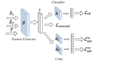
Figure 8: Network Structure of Proposed Approach. It consists three losses: the weighted Classification losses; the centroid matching for explicit conditional matching; the weighted adversarial loss for implicit conditional matching, showed in Eq. (4)

Where

• $\mathbf{C}_{t}^{y}=\sum_{(z_{t},y_{t})\sim\hat{\mathcal{S}}_{t}}\mathbf{1}_{\{y_{t}=y\}}z_{t}$ the centroid of label $Y=y$ in source $\mathcal{S}_{t}$.

• $\mathbf{C}^{y}=\sum_{(z_{t},y_{p})\sim\hat{\mathcal{T}}}\mathbf{1}_{\{y_{p}=y\}}z_{t}$ the centroid of pseudo-label $Y=y_{p}$ in target $\mathcal{S}_{t}$. (If it is the unsupervised DA scenarios).

• $\bar{\alpha}_{t}(z)=\mathbf{1}_{\{(z,y)\sim\mathcal{S}_{t}\}}\hat{\alpha}_{t}(Y=y)$, namely if each pair observation $(z,y)$ from the distribution, then $\bar{\alpha}_{t}(Z=z)=\hat{\alpha}_{t}(Y=y)$.

• $d_{1},\cdots,d_{T}$ are domain discriminator (or critic function) restricted within $1$-Lipschitz function.

• $\epsilon\in[0,1]$ is the adjustment parameter in the trade-off of explicit and implicit learning. We fix $\epsilon=0.5$ in the experiments.

• $\hat{\mathcal{T}}(y)$ empirical target label distribution. (In the unsupervised DA scenarios, we approximate it by predicted target label distribution $\bar{\mathcal{T}}(y)$.)

Gradient Penalty

In order to enforce the Lipschitz property of the statistic critic function, we adopt the gradient penalty term (Gulrajani et al., 2017). More concretely, given two samples $z_{s}\sim\mathcal{S}_{t}(z)$ and $z_{t}\sim\mathcal{T}(z)$ we generate an interpolated sample $z_{\text{int}}=\xi z_{s}+(1-\xi)z_{t}$ with $\xi\sim\text{Unif}[0,1]$. Then we add a gradient penalty $\|\nabla d(z_{\text{int}})\|^{2}_{2}$ as a regularization term to control the Lipschitz property w.r.t. the discriminator $d_{1},\cdots,d_{T}$.

Appendix K Algorithm Descriptions

We propose a detailed pipeline of the proposed algorithm in the following, shown in Algorithm 2 and 3. As for updating $\bm{\lambda}$ and $\alpha_{t}$, we iteratively solve the convex optimization problem after each training epoch and updating them by using the moving average technique.

For solving the $\bm{\lambda}$ and $\alpha_{t}$, we notice that frequently updating these two parameters in the mini-batch level will lead to an instability result during the training. As a consequence, we compute the accumulated confusion matrix, weighted prediction risk, and conditional Wasserstein distance for the whole training epoch and then solve the optimization problem. We use CVXPY to optimize the two standard convex losses.

Comparison with different time and memory complexity.

We discuss the time and memory complexity of our approach.

Time complexity: In computing each batch we need to compute $T$ re-weighted loss, $T$ domain adversarial loss and $T$ explicit conditional loss. Then our computational complexity is still $\mathcal{(}O)(T)$ during the mini-batch training, which is comparable with recent SOTA such as MDAN and DARN. In addition, after each training epoch we need to estimate $\alpha_{t}$ and $\bm{\lambda}$, which can have time complexity $\mathcal{O}(T|\mathcal{Y}|)$ with each epoch. (If we adopt SGD to solve these two convex problems). Therefore, the our proposed algorithm is time complexity $\mathcal{O}(T|\mathcal{Y}|)$. The extra $\mathcal{Y}$ term in time complexity is due to the approach of label shift in the designed algorithm.

Memory Complexity: Our proposed approach requires $\mathcal{O}(T)$ domain discriminator and $\mathcal{O}(T|\mathcal{Y}|)$ class-feature centroids. By the contrary, MDAN and DARN require $\mathcal{O}(T)$ domain discriminator and M3SDA and MDMN require $\mathcal{O}(T^{2})$ domain discriminators. Since our class-feature centroids are defined in the latent space ($z$), then the memory complexity of the class-feature centroids can be much smaller than domain discriminators.

Algorithm 2 Wasserstein Aggregation Domain Network (unsupervised scenarios, one iteration)

0:  Labeled source samples $\hat{\mathcal{S}}_{1},\dots,\hat{\mathcal{S}}_{T}$, Target samples $\hat{\mathcal{T}}$

0:  Label distribution ratio $\hat{\alpha}_{t}$ and task relation simplex $\bm{\lambda}$. Feature Learner $g$, Classifier $h$, Statistic critic function $d_{1},\dots,d_{T}$, class centroid for source $\mathbf{C}_{t}^{y}$ and target $\mathbf{C}^{y}$ ($\forall t=[1,T],y\in\mathcal{Y}$).

1:  $\triangleright\triangleright\triangleright$ DNN Parameter Training Stage (fixed $\alpha_{t}$ and $\bm{\lambda}$) $\triangleleft\triangleleft\triangleleft$

2:  for mini-batch of samples $(\mathbf{x}_{\mathcal{S}_{1}},\mathbf{y}_{\mathcal{S}_{1}})\sim\hat{\mathcal{S}}_{1}$, $\dots$, $(\mathbf{x}_{\mathcal{S}_{T}},\mathbf{y}_{\mathcal{S}_{T}})\sim\hat{\mathcal{S}}_{T}$, $(\mathbf{x}_{\mathcal{T}})\sim\hat{\mathcal{T}}$  do

3:     Predict target pseudo-label $\bar{\mathbf{y}}_{\mathcal{T}}=\text{argmax}_{y}h(g(\mathbf{x}_{\mathcal{T}}),y)$

4:     Compute source confusion matrix for each batch (un-normalized)       $C_{\hat{\mathcal{S}}_{t}}=\#[\text{argmax}_{y^{\prime}}h(z,y^{\prime})=y,Y=k]$ ($t=1,\dots,T$)

5:     Compute the batched class centroid for source $C_{t}^{y}$ and target $C^{y}$.

6:     Moving Average for update source/target class centroid: (We set $\epsilon_{1}=0.7$)

7:        Source class centroid update  $\mathbf{C}_{t}^{y}=\epsilon_{1}\times\mathbf{C}_{t}^{y}+(1-\epsilon_{1})\times C_{t}^{y}$

8:        Target class centroid update  $\mathbf{C}^{y}=\epsilon_{1}\times\mathbf{C}^{y}+(1-\epsilon_{1})\times C^{y}$

9:     Updating $g,h,d_{1},\dots,d_{T}$ (SGD and Gradient Reversal), based on Eq.(4)

10:  end for

11:  $\triangleright\triangleright\triangleright$ Estimation $\hat{\alpha}_{t}$ and $\bm{\lambda}$ $\triangleleft\triangleleft\triangleleft$

12:  Compute the global(normalized) source confusion matrix $C_{\hat{\mathcal{S}}_{t}}=\hat{\mathcal{S}}_{t}[\text{argmax}_{y^{\prime}}h(z,y^{\prime})=y,Y=k]$ ($t=1,\dots,T$)

13:  Solve $\alpha_{t}$ (denoted as $\{\alpha_{t}^{\prime}\}_{t=1}^{T}$) (Or Eq.(3)) in the partial scenario).

14:  Update $\alpha_{t}$ by moving average: $\alpha_{t}=\epsilon_{1}\times\alpha_{t}+(1-\epsilon_{1})\times\alpha_{t}^{\prime}$

15:  Compute the weighted loss and weighted centroid distance, then solve $\bm{\lambda}$ (denoted as $\bm{\lambda}^{\prime}$) from Sec. 2.3.

16:  Updating $\bm{\lambda}$ by moving average: $\bm{\lambda}=0.8\times\bm{\lambda}+0.2\times\bm{\lambda}^{\prime}$

Algorithm 3 Wasserstein Aggregation Domain Network (Limited Target Data, one iteration)

0:  Labeled source samples $\hat{\mathcal{S}}_{1},\dots,\hat{\mathcal{S}}_{T}$, Target samples $\hat{\mathcal{T}}$, Label shift ratio $\alpha_{t}$

0:  Task relation simplex $\bm{\lambda}$. Feature Learner $g$, Classifier $h$, Statistic critic function $d_{1},\dots,d_{T}$, class centroid for source $\mathbf{C}_{t}^{y}$ and target $\mathbf{C}^{y}$ ($\forall t=[1,T],y\in\mathcal{Y}$).

1:  $\triangleright\triangleright\triangleright$ DNN Parameter Training Stage (fixed $\bm{\lambda}$) $\triangleleft\triangleleft\triangleleft$

2:  for mini-batch of samples $(\mathbf{x}_{\mathcal{S}_{1}},\mathbf{y}_{\mathcal{S}_{1}})\sim\hat{\mathcal{S}}_{1}$, $\dots$, $(\mathbf{x}_{\mathcal{S}_{T}},\mathbf{y}_{\mathcal{S}_{T}})\sim\hat{\mathcal{S}}_{T}$, $(\mathbf{x}_{\mathcal{T}})\sim\hat{\mathcal{T}}$  do

3:     Compute the batched class centroid for source $C_{t}^{y}$ and target $C^{y}$.

4:     Moving Average for update source/target class centroid: (We set $\epsilon_{1}=0.7$)

5:        Source class centroid update  $\mathbf{C}_{t}^{y}=\epsilon_{1}\times\mathbf{C}_{t}^{y}+(1-\epsilon_{1})\times C_{t}^{y}$

6:        Target class centroid update  $\mathbf{C}^{y}=\epsilon_{1}\times\mathbf{C}^{y}+(1-\epsilon_{1})\times C^{y}$

7:     Updating $g,h,d_{1},\dots,d_{T}$ (SGD and Gradient Reversal), based on Eq.(4).

8:  end for

9:  $\triangleright\triangleright\triangleright$ Estimation $\bm{\lambda}$ $\triangleleft\triangleleft\triangleleft$

10:  Solve $\bm{\lambda}$ by Sec. 2.3. (denoted as $\bm{\lambda}^{\prime}$)

11:  Updating $\bm{\lambda}$ by moving average: $\bm{\lambda}=\epsilon_{1}\times\bm{\lambda}+(1-\epsilon_{1})\times\bm{\lambda}^{\prime}$

Appendix L Dataset Description and Experimental Details

L.1 Amazon Review Dataset

We used the amazon review dataset (Blitzer et al., 2007). It contains four domains (Books, DVD, Electronics, and Kitchen) with positive (label ”1”) and negative product reviews (label ”0”). The data size is 6465 (Books), 5586 (DVD), 7681 (Electronics), and 7945 (Kitchen). We follow the common data pre-processing strategies (Chen et al., 2012): use the bag-of-words (BOW) features then extract the top-5000 frequent unigram and bigrams of all the reviews.

We also noticed the original data-set are label balanced $\mathcal{D}(y=0)=\mathcal{D}(y=1)$. To enhance the benefits of the proposed approach, we create a new dataset with label distribution drift. Specifically, in the experimental settings, we randomly drop $50\%$ data with label ”0” (negative reviews) for all the source data while keeping the target identical, showing in Fig (9).

We choose the MLP model with

• feature representation function $g$: $[5000,1000]$ units

• Task prediction and domain discriminator function $[1000,500,100]$ units,

We choose the dropout rate as $0.7$ in the hidden and input layers. The hyper-parameters are chosen based on cross-validation. The neural network is trained for $50$ epochs and the mini-batch size is 20 per domain. The optimizer is Adadelta with a learning rate of 0.5.

Experimental Setting

We use the amazon Review dataset for two transfer learning scenarios (limited target labels and unsupervised DA). We first randomly select 2K samples for each domain. Then we create a drifted distribution of each source, making each source $\approx 1500$ and target sample still 2K.

In the unsupervised DA, we use these labeled source tasks and unlabelled target task, which aims to predict the labels on the target domain.

In the conventional transfer learning, we random sample only $10\%$ dataset ($\approx 200$ samples) as the target training set and the rest $90\%$ samples as the target test set.

We select $C_{0}=0.01$ and $C_{1}=1$ for these two transfer scenarios. In both practical settings, we set the maximum training epoch as 50.

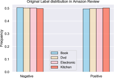
(a)

(b)

Figure 9: Amazon Review dataset (a) Original Label Training Distribution; (b) Label-Shifted distribution with sources tasks: Book, Dvd, Electronic, and target task Kitchen. We randomly drop $50\%$ of the negative reviews for all the source distribution while keeping the target label distribution unchanged.

L.2 Digit Recognition

We follow the same settings of (Ganin et al., 2016) and we use four-digit recognition datasets in the experiments MNIST, USPS, SVHN, and Synth. MNIST and USPS are the standard digits recognition task. Street View House Number (SVHN) (Ganin et al., 2016) is the digit recognition dataset from house numbers in Google Street View Images. Synthetic Digits (Synth) (Ganin et al., 2016) is a synthetic dataset that by various transforming SVHN dataset.

We also visualize the label distribution in these four datasets. The original datasets show an almost uniform label distribution on the MNIST as well as Synth, (showing in Fig. 11 (a)). In our paper, we generate a label distribution drift on the source datasets for each multi-source transfer learning. Concretely, we drop $50\%$ of the data on digits 5-9 of all the sources while we keep the target label distribution unchanged. (Fig. 11 (b) illustrated one example with sources: Mnist, USPS, SVHN, and Target Synth. We drop the labels only on the sources.)

MNIST and USPS images are resized to 32 $\times$ 32 and represented as 3-channel color images to match the shape of the other three datasets. Each domain has its own given training and test sets when downloaded. Their respective training sample sizes are 60000, 7219, 73257, 479400, and the respective test sample sizes are 10000, 2017, 26032, 9553.

The model structure is shown in Fig. 10. There is no dropout and the hyperparameters are chosen based on cross-validation. It is trained for 60 epochs and the mini-batch size is 128 per domain. The optimizer is Adadelta with a learning rate of 1.0. We adopted $\gamma=0.5$ for MDAN and $\gamma=0.1$ for DARN in the baseline (Wen et al., 2020).

Experimental Setting

We use the Digits dataset for two transfer learning scenarios (limited target labels and unsupervised DA). Notice the USPS data has only 7219 samples and the digits dataset is relatively simple. We first randomly select 7K samples for each domain. We create a drifted distribution of each source, making each source $\approx 5300$, and the target sample still 7K.

In the unsupervised DA, we use these labeled source tasks and unlabelled target task, which aims to predict the labels on the target domain.

In the transfer learning with limited data, we random sample only $10\%$ dataset ($\approx 700$ samples) as the target training set and the rest $90\%$ samples as the target test set.

We select $C_{0}=0.01$ and $C_{1}$ as the maximum prediction loss $C_{1}=\max_{t}{R^{\alpha_{t}}(h)}$ as the hyper-parameters across these two scenarios. The maximum training epoch is $60$.

1. Feature extractor: with 3 convolution layers.

   ’layer1’: ’conv’: [3, 3, 64], ’relu’: [], ’maxpool’: [2, 2, 0],

   ’layer2’: ’conv’: [3, 3, 128], ’relu’: [], ’maxpool’: [2, 2, 0],

   ’layer3’: ’conv’: [3, 3, 256], ’relu’: [], ’maxpool’: [2, 2, 0],

2. Task prediction: with 3 fully connected layers.

   ’layer1’: ’fc’: [*, 512], ’act_fn’: ’relu’,

   ’layer2’: ’fc’: [512, 100], ’act_fn’: ’relu’,

   ’layer3’: ’fc’: [100, 10],

3. Domain Discriminator: with 2 fully connected layers.

   reverse_gradient()

   ’layer1’: ’fc’: [*, 256], ’act_fn’: ’relu’,

   ’layer2’: ’fc’: [256, 1],

Figure 10: Neural Network Structure in the digits recognition (Ganin et al., 2016)

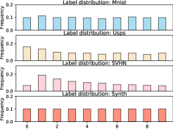
(a)

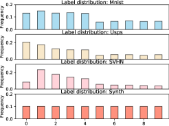
(b)

Figure 11: One example in Digits dataset with Sources: MNIST, USPS, SVHN and Target Synth. We randomly drop $50\%$ data on digits 5-9 in all sources while keeping target label distribution unchanged.

L.3 Office-Home dataset

To show the dataset in the complex scenarios, we use the challenging Office-Home dataset (Venkateswara et al., 2017). It contains images of 65 objects such as a spoon, sink, mug, and pen from four different domains: Art (paintings, sketches, and/or artistic depictions), Clipart (clipart images), Product (images without background), and Real-World (regular images captured with a camera). One of the four datasets is chosen as an unlabelled target domain and the other three datasets are used as labeled source domains.

The dataset size is 2427 (Art), 4365 (Clipart), 4439 (Product), 4357 (Real-World). We follow the same training/test procedure as (Wen et al., 2020). We additionally visualize the label distribution $\mathcal{D}(y)$ in four domains in Fig.3, which illustrated the inherent different label distributions. We did not re-sample the source label distribution to uniform distribution in the data pre-processing step. All the baselines are evaluated under the same setting.

We use the ResNet50 (He et al., 2016) pretrained from the ImageNet in PyTorch as the base network for feature learning and put an MLP with the network structure shown in Fig. 12.

Experimental Settings

We use the original Office-Home dataset for two transfer learning scenarios (unsupervised DA and label-partial unsupervised DA). We use SGD optimizer with learning rate 0.005, momentum 0.9 and weight_decay value 1e-3. It is trained for 100 epochs and the mini-batch size is 32 per domain. As for the baselines, MDAN use $\gamma$ = 1.0 while DARN use $\gamma$ = 0.5. We select $C_{0}=0.01$ and $C_{1}$ as the maximum prediction loss $C_{1}=\max_{t}{R^{\alpha_{t}}(h)}$ as the hyper-parameters across these two scenarios.

In the multi-source unsupervised partial DA, we randomly select 35 classes from the target (by repeating 3 samplings), then at each sampling we run 5 times. The final result is based on these $3\times 5=15$ repetitions.

1. Feature extractor: ResNet50 (He et al., 2016),

2. Task prediction: with 3 fully connected layers.

   ’layer1’: ’fc’: [*, 256], ’batch_normalization’, ’act_fn’: ’Leaky_relu’,

   ’layer2’: ’fc’: [256, 256], ’batch_normalization’, ’act_fn’: ’Leaky_relu’,

   ’layer3’: ’fc’: [256, 65],

3. Domain Discriminator: with 3 fully connected layers.

   reverse_gradient()

   ’layer1’: ’fc’: [*, 256], ’batch_normalization’, ’act_fn’: ’Leaky_relu’,

   ’layer2’: ’fc’: [256, 256], ’batch_normalization’, ’act_fn’: ’Leaky_relu’,

   ’layer3’: ’fc’: [256, 1], ’Sigmoid’,

Figure 12: Neural Network Structure in the Office-Home

Appendix M Analysis in Unsupervised DA

M.1 Ablation Study: Different Dropping Rate

To show the effectiveness of our proposed approach, we change the drop rate of the source domains, showing in Fig.(13). We observe that in task Book, DVD, Electronic, and Kitchen, the results are significantly better under a large label-shift. In the initialization with almost no label shift, the state-of-the-art DARN illustrates a slightly better ($<1\%$) result.

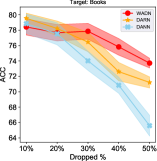
(a) Target: Book

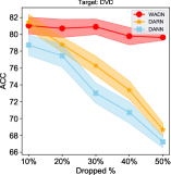
(b) Target: DVD

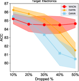
(c) Target: Electronics

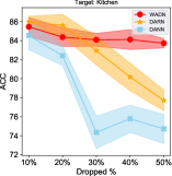
(d) Target: Kitchen

Figure 13: Different label drift levels on Amazon Dataset. Larger dropping rate means higher label shift.

M.2 Additional Analysis on Amazon Dataset

We present two additional results to illustrate the working principles of WADN, showing in Fig. (14).

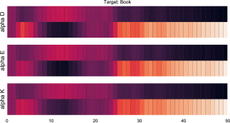
(a) Target: Book

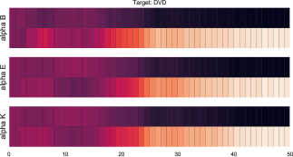
(b) Target: DVD

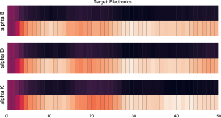
(c) Target: Electronics

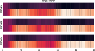
(d) Target: Kitchen

Figure 14: Amazon Dataset. WADN approach: evolution of $\hat{\alpha}_{t}$ during the training. Darker indicates higher Value. Since we drop $y=0$ in the sources, then the true $\alpha_{t}(0)>1$ will be assigned with higher value.

We visualize the evolution of $\bm{\lambda}$ between DARN and WADN, which both used theoretical principled approach to estimate $\bm{\lambda}$. We observe that in the source shifted data, DARN shows an inconsistent estimator of $\bm{\lambda}$. This is different from the observation of (Wen et al., 2020). We think it may in the conditional and label distribution shift problem, using $\hat{R}_{\mathcal{S}}(h(z))+\text{Discrepancy}(\mathcal{S}(z),\mathcal{T}(z))$ to update $\bm{\lambda}$ is unstable. In contrast, WADN illustrates a relative consistent estimator of $\bm{\lambda}$ under the source shifted data.

In addition, WARN gradually and correctly estimates the unbalanced source data and assign higher wights $\alpha_{t}$ for label $y=0$ (first row of Fig.(14)). These principles in WADN jointly promote significantly better results.

M.3 Additional Analysis on Digits Dataset

We show the evolution of $\hat{\alpha}_{t}$ on WADN, which verifies the correctness of our proposed principle. Since we drop digits 5-9 in the source domains, the results in Fig. (15) illustrate a higher $\hat{\alpha}_{t}$ on these digits.

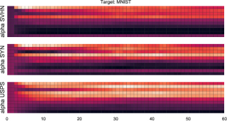
(a) Target: MNIST

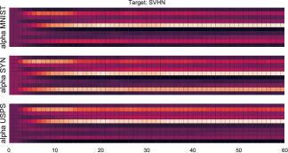
(b) Target: SVHN

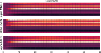
(c) Target: Synth

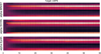
(d) Target: USPS

Figure 15: Digits Dataset. WADN approach: evolution of $\hat{\alpha}_{t}$ during the training. Darker indicates higher value. Since we drop digits $5-9$ on source domain, therefore, $\alpha_{t}(y)$, $y\in[5,9]$ will be assigned with a relative higher value.

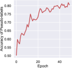
(a) Amazon Review: target DVDs

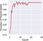
(b) Digits: target SVHN

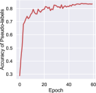
(c) Digits: target Synth

Figure 16: Evolution of accuracy w.r.t. the predicted target pseudo-labels in different tasks in unsupervised DA.

Appendix N Partial multi-source Unsupervised DA

From Fig. (17), WADN is consistently better than other baselines, given different selected classes.

Besides, when fewer classes are selected, the accuracy in DANN, PADA, and DARN is not drastically dropping but maintaining a relatively stable result. We think the following possible reasons:

• The reported performances are based on the average of different selected sub-classes rather than one sub-class selection. From the statistical perspective, if we take a close look at the variance, the results in DANN are much more unstable (higher std) inducing by the different samplings. Therefore, the conventional domain adversarial training is improper for handling the partial transfer since it is not reliable and negative transfer still occurs.

• In multi-source DA, it is equally important to detect the non-overlapping classes and find the most similar sources. Comparing the baselines that only focus on one or two principles shows the importance of unified principles in multi-source partial DA.

• We also observe that in the Real-World dataset, the DANN improves the performance by a relatively large value. This is due to the inherent difficultly of the learning task itself. In fact, the Real-World domain illustrates a much higher performance compared with other domains. According to the Fano lower bound, a task with smaller classes is generally easy to learn. It is possible the vanilla approach showed improvement but still with a much higher variance.

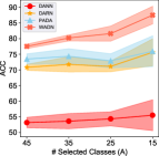
(a) Target: Art

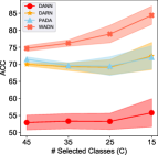
(b) Target: Clipart

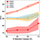
(c) Target: Real-World

Figure 17: Multi-source Label Partial DA: Performance with different target selected classes.

Fig (18), (19) showed the estimated $\hat{\alpha}_{t}$ with different selected classes. The results validate the correctness of WADN in estimating the label distribution ratio.

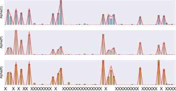
(a) Target: Art

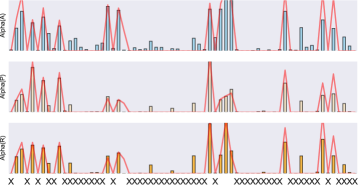
(b) Target: Clipart

(c) Target: Product

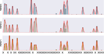
(d) Target: Real-World

Figure 18: We select 15 classes and visualize estimated $\hat{\alpha}_{t}$ (the bar plot). The ”X” along the x-axis represents the index of dropped 50 classes. The red curves are the ground-truth label distribution ratio.

(a) Target: Art

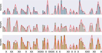
(b) Target: Clipart

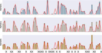
(c) Target: Product

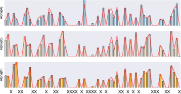
(d) Target: Real-World

Figure 19: We select 35 classes and visualize estimated $\hat{\alpha}_{t}$ (the bar plot). The ”X” along the x-axis represents the index of dropped 30 classes. The red curves are the ground-truth label distribution ratio.

References

- Akuzawa et al. (2019) Akuzawa, K., Iwasawa, Y., and Matsuo, Y. Adversarial invariant feature learning with accuracy constraint for domain generalization. In Joint European Conference on Machine Learning and Knowledge Discovery in Databases, pp. 315–331. Springer, 2019.
- Arjovsky et al. (2017) Arjovsky, M., Chintala, S., and Bottou, L. Wasserstein gan. arXiv preprint arXiv:1701.07875, 2017.
- Azizzadenesheli et al. (2019) Azizzadenesheli, K., Liu, A., Yang, F., and Anandkumar, A. Regularized learning for domain adaptation under label shifts. In International Conference on Learning Representations, 2019. URL https://openreview.net/forum?id=rJl0r3R9KX.
- Balaji et al. (2018) Balaji, Y., Sankaranarayanan, S., and Chellappa, R. Metareg: Towards domain generalization using meta-regularization. In Advances in Neural Information Processing Systems, pp. 998–1008, 2018.
- Balaji et al. (2019) Balaji, Y., Chellappa, R., and Feizi, S. Normalized wasserstein distance for mixture distributions with applications in adversarial learning and domain adaptation. arXiv preprint arXiv:1902.00415, 2019.
- Ben-David et al. (2007) Ben-David, S., Blitzer, J., Crammer, K., and Pereira, F. Analysis of representations for domain adaptation. In Advances in neural information processing systems, pp. 137–144, 2007.
- Ben-David et al. (2010a) Ben-David, S., Blitzer, J., Crammer, K., Kulesza, A., Pereira, F., and Vaughan, J. W. A theory of learning from different domains. Machine learning, 79(1-2):151–175, 2010a.
- Ben-David et al. (2010b) Ben-David, S., Lu, T., Luu, T., and Pál, D. Impossibility theorems for domain adaptation. In International Conference on Artificial Intelligence and Statistics, pp. 129–136, 2010b.
- Blitzer et al. (2007) Blitzer, J., Dredze, M., and Pereira, F. Biographies, bollywood, boom-boxes and blenders: Domain adaptation for sentiment classification. In Proceedings of the 45th annual meeting of the association of computational linguistics, pp. 440–447, 2007.
- Bucci et al. (2019) Bucci, S., D’Innocente, A., and Tommasi, T. Tackling partial domain adaptation with self-supervision. In International Conference on Image Analysis and Processing, pp. 70–81. Springer, 2019.
- Cao et al. (2018) Cao, Z., Ma, L., Long, M., and Wang, J. Partial adversarial domain adaptation. In Proceedings of the European Conference on Computer Vision (ECCV), pp. 135–150, 2018.
- Cao et al. (2019) Cao, Z., You, K., Long, M., Wang, J., and Yang, Q. Learning to transfer examples for partial domain adaptation. In Proceedings of the IEEE Conference on Computer Vision and Pattern Recognition, pp. 2985–2994, 2019.
- Chapelle & Zien (2005) Chapelle, O. and Zien, A. Semi-supervised classification by low density separation. In AISTATS, volume 2005, pp. 57–64. Citeseer, 2005.
- Chen et al. (2012) Chen, M., Xu, Z., Weinberger, K. Q., and Sha, F. Marginalized denoising autoencoders for domain adaptation. In Proceedings of the 29th International Coference on International Conference on Machine Learning, pp. 1627–1634, 2012.
- Chen et al. (2019) Chen, X., Awadallah, A. H., Hassan, H., Wang, W., and Cardie, C. Multi-source cross-lingual model transfer: Learning what to share. In Proceedings of the 57th Annual Meeting of the Association for Computational Linguistics, 2019.
- Chen et al. (2020) Chen, Z., Chen, C., Cheng, Z., Fang, K., and Jin, X. Selective transfer with reinforced transfer network for partial domain adaptation. In AAAI Conference on Artificial Intelligence, 2020.
- Christodoulidis et al. (2016) Christodoulidis, S., Anthimopoulos, M., Ebner, L., Christe, A., and Mougiakakou, S. Multisource transfer learning with convolutional neural networks for lung pattern analysis. IEEE journal of biomedical and health informatics, 21(1):76–84, 2016.
- Combes et al. (2020) Combes, R. T. d., Zhao, H., Wang, Y.-X., and Gordon, G. Domain adaptation with conditional distribution matching and generalized label shift. arXiv preprint arXiv:2003.04475, 2020.
- Ganin et al. (2016) Ganin, Y., Ustinova, E., Ajakan, H., Germain, P., Larochelle, H., Laviolette, F., Marchand, M., and Lempitsky, V. Domain-adversarial training of neural networks. The Journal of Machine Learning Research, 17(1):2096–2030, 2016.
- Garg et al. (2020) Garg, S., Wu, Y., Balakrishnan, S., and Lipton, Z. C. A unified view of label shift estimation. arXiv preprint arXiv:2003.07554, 2020.
- Geiss et al. (2014) Geiss, L. S., Wang, J., Cheng, Y. J., Thompson, T. J., Barker, L., Li, Y., Albright, A. L., and Gregg, E. W. Prevalence and incidence trends for diagnosed diabetes among adults aged 20 to 79 years, united states, 1980-2012. Jama, 312(12):1218–1226, 2014.
- Gong et al. (2016) Gong, M., Zhang, K., Liu, T., Tao, D., Glymour, C., and Schölkopf, B. Domain adaptation with conditional transferable components. In International conference on machine learning, pp. 2839–2848, 2016.
- Gulrajani et al. (2017) Gulrajani, I., Ahmed, F., Arjovsky, M., Dumoulin, V., and Courville, A. C. Improved training of wasserstein gans. In Advances in Neural Information Processing Systems, pp. 5767–5777, 2017.
- He et al. (2016) He, K., Zhang, X., Ren, S., and Sun, J. Deep residual learning for image recognition. In Proceedings of the IEEE conference on computer vision and pattern recognition, pp. 770–778, 2016.
- Hoffman et al. (2012) Hoffman, J., Kulis, B., Darrell, T., and Saenko, K. Discovering latent domains for multisource domain adaptation. In European Conference on Computer Vision, pp. 702–715. Springer, 2012.
- Hoffman et al. (2018a) Hoffman, J., Mohri, M., and Zhang, N. Algorithms and theory for multiple-source adaptation. In Advances in Neural Information Processing Systems, pp. 8246–8256, 2018a.
- Hoffman et al. (2018b) Hoffman, J., Tzeng, E., Park, T., Zhu, J.-Y., Isola, P., Saenko, K., Efros, A., and Darrell, T. Cycada: Cycle-consistent adversarial domain adaptation. In International conference on machine learning, pp. 1989–1998. PMLR, 2018b.
- Houlsby et al. (2019) Houlsby, N., Giurgiu, A., Jastrzebski, S., Morrone, B., De Laroussilhe, Q., Gesmundo, A., Attariyan, M., and Gelly, S. Parameter-efficient transfer learning for nlp. arXiv preprint arXiv:1902.00751, 2019.
- Hull (1994) Hull, J. J. A database for handwritten text recognition research. IEEE Transactions on pattern analysis and machine intelligence, 16(5):550–554, 1994.
- Ilse et al. (2019) Ilse, M., Tomczak, J. M., Louizos, C., and Welling, M. Diva: Domain invariant variational autoencoders. arXiv preprint arXiv:1905.10427, 2019.
- Johansson et al. (2019) Johansson, F., Sontag, D., and Ranganath, R. Support and invertibility in domain-invariant representations. In The 22nd International Conference on Artificial Intelligence and Statistics, pp. 527–536, 2019.
- Konstantinov & Lampert (2019) Konstantinov, N. and Lampert, C. Robust learning from untrusted sources. In International Conference on Machine Learning, pp. 3488–3498, 2019.
- Lee et al. (2019) Lee, J., Sattigeri, P., and Wornell, G. Learning new tricks from old dogs: Multi-source transfer learning from pre-trained networks. In Advances in Neural Information Processing Systems, pp. 4370–4380, 2019.
- Li et al. (2018a) Li, H., Jialin Pan, S., Wang, S., and Kot, A. C. Domain generalization with adversarial feature learning. In Proceedings of the IEEE Conference on Computer Vision and Pattern Recognition, pp. 5400–5409, 2018a.
- Li et al. (2019a) Li, J., Wu, W., Xue, D., and Gao, P. Multi-source deep transfer neural network algorithm. Sensors, 19(18):3992, 2019a.
- Li et al. (2018b) Li, Y., Carlson, D. E., et al. Extracting relationships by multi-domain matching. In Advances in Neural Information Processing Systems, pp. 6798–6809, 2018b.
- Li et al. (2018c) Li, Y., Tian, X., Gong, M., Liu, Y., Liu, T., Zhang, K., and Tao, D. Deep domain generalization via conditional invariant adversarial networks. In Proceedings of the European Conference on Computer Vision (ECCV), pp. 624–639, 2018c.
- Li et al. (2019b) Li, Y., Murias, M., Major, S., Dawson, G., and Carlson, D. On target shift in adversarial domain adaptation. In The 22nd International Conference on Artificial Intelligence and Statistics, pp. 616–625, 2019b.
- Lin et al. (2020) Lin, C., Zhao, S., Meng, L., and Chua, T.-S. Multi-source domain adaptation for visual sentiment classification. arXiv preprint arXiv:2001.03886, 2020.
- Lipton et al. (2018) Lipton, Z., Wang, Y.-X., and Smola, A. Detecting and correcting for label shift with black box predictors. In International Conference on Machine Learning, pp. 3122–3130, 2018.
- Liu et al. (2004) Liu, J., Hong, Y., D’Agostino Sr, R. B., Wu, Z., Wang, W., Sun, J., Wilson, P. W., Kannel, W. B., and Zhao, D. Predictive value for the chinese population of the framingham chd risk assessment tool compared with the chinese multi-provincial cohort study. Jama, 291(21):2591–2599, 2004.
- Mansour et al. (2009a) Mansour, Y., Mohri, M., and Rostamizadeh, A. Domain adaptation: Learning bounds and algorithms. arXiv preprint arXiv:0902.3430, 2009a.
- Mansour et al. (2009b) Mansour, Y., Mohri, M., and Rostamizadeh, A. Multiple source adaptation and the rényi divergence. In Proceedings of the Twenty-Fifth Conference on Uncertainty in Artificial Intelligence, pp. 367–374. AUAI Press, 2009b.
- Mansour et al. (2020) Mansour, Y., Mohri, M., Suresh, A. T., and Wu, K. A theory of multiple-source adaptation with limited target labeled data. arXiv preprint arXiv:2007.09762, 2020.
- Mohri & Medina (2012) Mohri, M. and Medina, A. M. New analysis and algorithm for learning with drifting distributions. In International Conference on Algorithmic Learning Theory, pp. 124–138. Springer, 2012.
- Motiian et al. (2017) Motiian, S., Piccirilli, M., Adjeroh, D. A., and Doretto, G. Unified deep supervised domain adaptation and generalization. In The IEEE International Conference on Computer Vision (ICCV), Oct 2017.
- Netzer et al. (2011) Netzer, Y., Wang, T., Coates, A., Bissacco, A., Wu, B., and Ng, A. Y. Reading digits in natural images with unsupervised feature learning. 2011.
- Nguyen et al. (2009) Nguyen, X., Wainwright, M. J., Jordan, M. I., et al. On surrogate loss functions and f-divergences. The Annals of Statistics, 37(2):876–904, 2009.
- Pan & Yang (2009) Pan, S. J. and Yang, Q. A survey on transfer learning. IEEE Transactions on knowledge and data engineering, 22(10):1345–1359, 2009.
- Pei et al. (2018) Pei, Z., Cao, Z., Long, M., and Wang, J. Multi-adversarial domain adaptation. arXiv preprint arXiv:1809.02176, 2018.
- Peng et al. (2019) Peng, X., Bai, Q., Xia, X., Huang, Z., Saenko, K., and Wang, B. Moment matching for multi-source domain adaptation. In Proceedings of the IEEE International Conference on Computer Vision, pp. 1406–1415, 2019.
- Raghu et al. (2019) Raghu, M., Zhang, C., Kleinberg, J., and Bengio, S. Transfusion: Understanding transfer learning for medical imaging. In Advances in neural information processing systems, pp. 3347–3357, 2019.
- Redko et al. (2019) Redko, I., Courty, N., Flamary, R., and Tuia, D. Optimal transport for multi-source domain adaptation under target shift. In Chaudhuri, K. and Sugiyama, M. (eds.), Proceedings of Machine Learning Research, volume 89 of Proceedings of Machine Learning Research, pp. 849–858. PMLR, 16–18 Apr 2019. URL http://proceedings.mlr.press/v89/redko19a.html.
- Ruder (2017) Ruder, S. An overview of multi-task learning in deep neural networks. arXiv preprint arXiv:1706.05098, 2017.
- Ruder et al. (2019) Ruder, S., Peters, M. E., Swayamdipta, S., and Wolf, T. Transfer learning in natural language processing. In Proceedings of the 2019 Conference of the North American Chapter of the Association for Computational Linguistics: Tutorials, pp. 15–18, 2019.
- Saenko et al. (2010) Saenko, K., Kulis, B., Fritz, M., and Darrell, T. Adapting visual category models to new domains. In European conference on computer vision, pp. 213–226. Springer, 2010.
- Saito et al. (2018) Saito, K., Watanabe, K., Ushiku, Y., and Harada, T. Maximum classifier discrepancy for unsupervised domain adaptation. In Proceedings of the IEEE Conference on Computer Vision and Pattern Recognition, pp. 3723–3732, 2018.
- Saito et al. (2019) Saito, K., Kim, D., Sclaroff, S., Darrell, T., and Saenko, K. Semi-supervised domain adaptation via minimax entropy. In Proceedings of the IEEE International Conference on Computer Vision, pp. 8050–8058, 2019.
- Sankaranarayanan et al. (2018) Sankaranarayanan, S., Balaji, Y., Castillo, C. D., and Chellappa, R. Generate to adapt: Aligning domains using generative adversarial networks. In Proceedings of the IEEE Conference on Computer Vision and Pattern Recognition, pp. 8503–8512, 2018.
- Shalev-Shwartz & Ben-David (2014) Shalev-Shwartz, S. and Ben-David, S. Understanding machine learning: From theory to algorithms. Cambridge university press, 2014.
- Shui et al. (2019) Shui, C., Abbasi, M., Robitaille, L.-É., Wang, B., and Gagné, C. A principled approach for learning task similarity in multitask learning. In Proceedings of the Twenty-Eighth International Joint Conference on Artificial Intelligence, pp. 3446–3452, 2019.
- Stojanov et al. (2019) Stojanov, P., Gong, M., Carbonell, J. G., and Zhang, K. Data-driven approach to multiple-source domain adaptation. Proceedings of machine learning research, 89:3487, 2019.
- Sugiyama & Kawanabe (2012) Sugiyama, M. and Kawanabe, M. Machine learning in non-stationary environments: Introduction to covariate shift adaptation. MIT press, 2012.
- Tan et al. (2013) Tan, B., Zhong, E., Xiang, E. W., and Yang, Q. Multi-transfer: Transfer learning with multiple views and multiple sources. In Proceedings of the 2013 SIAM International Conference on Data Mining, pp. 243–251. SIAM, 2013.
- Venkateswara et al. (2017) Venkateswara, H., Eusebio, J., Chakraborty, S., and Panchanathan, S. Deep hashing network for unsupervised domain adaptation. In Proceedings of the IEEE Conference on Computer Vision and Pattern Recognition, pp. 5018–5027, 2017.
- Wang et al. (2019a) Wang, B., Mendez, J., Cai, M., and Eaton, E. Transfer learning via minimizing the performance gap between domains. In Advances in Neural Information Processing Systems, pp. 10645–10655, 2019a.
- Wang et al. (2019b) Wang, B., Zhang, H., Liu, P., Shen, Z., and Pineau, J. Multitask metric learning: Theory and algorithm. In Proceedings of the International Conference on Artificial Intelligence and Statistics, pp. 3362–3371, 2019b.
- Wang et al. (2020) Wang, B., Wong, C. M., Kang, Z., Liu, F., Shui, C., Wan, F., and Chen, C. P. Common spatial pattern reformulated for regularizations in brain-computer interfaces. IEEE Transactions on Cybernetics, 2020.
- Wang et al. (2019c) Wang, H., Yang, W., Lin, Z., and Yu, Y. Tmda: Task-specific multi-source domain adaptation via clustering embedded adversarial training. In 2019 IEEE International Conference on Data Mining (ICDM), pp. 1372–1377. IEEE, 2019c.
- Weed et al. (2019) Weed, J., Bach, F., et al. Sharp asymptotic and finite-sample rates of convergence of empirical measures in wasserstein distance. Bernoulli, 25(4A):2620–2648, 2019.
- Wei et al. (2017) Wei, P., Sagarna, R., Ke, Y., Ong, Y.-S., and Goh, C.-K. Source-target similarity modelings for multi-source transfer gaussian process regression. In International Conference on Machine Learning, pp. 3722–3731, 2017.
- Wen et al. (2020) Wen, J., Greiner, R., and Schuurmans, D. Domain aggregation networks for multi-source domain adaptation. Proceedings of the 37th International Conference on Machine Learning, 2020.
- Wu et al. (2019) Wu, Y., Winston, E., Kaushik, D., and Lipton, Z. Domain adaptation with asymmetrically-relaxed distribution alignment. In International Conference on Machine Learning, pp. 6872–6881, 2019.
- Yao & Doretto (2010) Yao, Y. and Doretto, G. Boosting for transfer learning with multiple sources. In 2010 IEEE Computer Society Conference on Computer Vision and Pattern Recognition, pp. 1855–1862. IEEE, 2010.
- Zhang et al. (2018) Zhang, J., Ding, Z., Li, W., and Ogunbona, P. Importance weighted adversarial nets for partial domain adaptation. In Proceedings of the IEEE Conference on Computer Vision and Pattern Recognition, pp. 8156–8164, 2018.
- Zhang et al. (2019) Zhang, J., Li, W., Ogunbona, P., and Xu, D. Recent advances in transfer learning for cross-dataset visual recognition: A problem-oriented perspective. ACM Computing Surveys (CSUR), 52(1):1–38, 2019.
- Zhang et al. (2013) Zhang, K., Schölkopf, B., Muandet, K., and Wang, Z. Domain adaptation under target and conditional shift. In International Conference on Machine Learning, pp. 819–827, 2013.
- Zhang & Yang (2017) Zhang, Y. and Yang, Q. A survey on multi-task learning. arXiv preprint arXiv:1707.08114, 2017.
- Zhang & Yeung (2012) Zhang, Y. and Yeung, D.-Y. A convex formulation for learning task relationships in multi-task learning. arXiv preprint arXiv:1203.3536, 2012.
- Zhao et al. (2018) Zhao, H., Zhang, S., Wu, G., Moura, J. M., Costeira, J. P., and Gordon, G. J. Adversarial multiple source domain adaptation. In Advances in neural information processing systems, pp. 8559–8570, 2018.
- Zhao et al. (2019) Zhao, S., Wang, G., Zhang, S., Gu, Y., Li, Y., Song, Z., Xu, P., Hu, R., Chai, H., and Keutzer, K. Multi-source distilling domain adaptation. arXiv preprint arXiv:1911.11554, 2019.
- Zhao et al. (2020) Zhao, S., Li, B., Xu, P., and Keutzer, K. Multi-source domain adaptation in the deep learning era: A systematic survey. arXiv preprint arXiv:2002.12169, 2020.
- Zhu et al. (2019) Zhu, Y., Zhuang, F., and Wang, D. Aligning domain-specific distribution and classifier for cross-domain classification from multiple sources. In Proceedings of the AAAI Conference on Artificial Intelligence, volume 33, pp. 5989–5996, 2019.