Gaia 400,894 QSO constraint on the energy density of
low-frequency gravitational waves

Abstract

Low frequency gravitational waves (GWs) are keys to understanding cosmological inflation and super massive blackhole (SMBH) formation via blackhole mergers, while it is difficult to identify the low frequency GWs with ground-based GW experiments such as the advanced LIGO (aLIGO) and VIRGO due to the seismic noise. Although quasi-stellar object (QSO) proper motions produced by the low frequency GWs are measured by pioneering studies of very long baseline interferometry (VLBI) observations with good positional accuracy, the low frequency GWs are not strongly constrained by the small statistics with 711 QSOs (Darling et al. 2018). Here we present the proper motion field map of 400,894 QSOs of the Sloan Digital Sky Survey (SDSS) with optical Gaia EDR3 proper motion measurements whose positional accuracy is $<0.4$ milli-arcsec comparable with the one of the radio VLBI observations. We obtain the best-fit spherical harmonics with the typical field strength of $\mathcal{O}(0.1)\,\mu$arcsec, and place a tight constraint on the energy density of GWs, $\Omega_{\rm gw}=(0.964\pm 3.804)\times 10^{-4}$ (95 % confidence level), that is significantly stronger than the one of the previous VLBI study by two orders of magnitude at the low frequency regime of $f<10^{-9}\,{\rm[Hz]}\simeq(30\,{\rm yr})^{-1}$ unexplored by the pulsar timing technique. Our upper limit rules out the existence of SMBH binary systems at the distance $r<400$ kpc from the Earth where the Milky Way center and local group galaxies are included. Demonstrating the limit given by our optical QSO study, we claim that astrometric satellite data including the forthcoming Gaia DR5 data with small systematic errors are powerful to constrain low frequency GWs.

I Introduction

Existence of gravitational waves (GWs) is one of the primary predictions of general relativity. Due to little interaction with matter on the line of sight, one can directly investigate the nature of sources in the strong gravitational fields such as mergers of binaries of blackholes and the cosmological inflation. However, because the strain amplitude of GWs is expected to be very small $\lesssim 10^{-24}$, there are many difficulties in the direct detection of GWs.

About one century has been past to detect GWs directly since the prediction about the existence of GWs. In 2015, GWs are directly detected for the first time with a laser interferometer named the advanced LIGO (aLIGO) [1]. With the event named GW150914, the existences of GWs as well as a binary blackhole merger have been observationally confirmed. In addition, in 2017, GWs from a binary neutron star (NS) merger are detected with aLIGO and Virgo. This binary NS merger is named GW170817. Simultaneously, the optical counterpart of GW170817, GRB170817A (AT2017gfo), is detected at a wide frequency range from gamma-ray to radio waves. Because the gamma ray from GRB170817A is detected only 1.7 seconds after the GW-signal detections, it is confirmed that the speed of GWs $c_{\rm gw}$ is the same as the speed of light $c$ with $10^{-15}$ accuracy [2]. These observations reject the modified gravity theories which predict $c_{\rm gw}\neq c$ [3, 4]. As a result, for example, the covariant Galileon (e.g. [5]) and the Gauss-Bonnet gravity (see [6]) are ruled out, and one needs an alternative theoretical framework for the accelerating expansion of the current Universe. The event GW170817/GRB170817A also provides a new standard ruler to astronomy because the absolute luminosity of the NS binary merger is estimated by numerical relativity and hydrodynamical simulations with the effects of general relativity. Due to the nature of the Hubble-Lemaître law, the standard ruler can be used to estimate the Hubble constant. The Hubble constant is successfully measured with GW170817/GRB170817A by these studies [7, 8]. These studies prove that GW astronomy provides a new and powerful ruler in the Universe. By measuring more than 10 NS binary mergers in the future, the Hubble constant will be determined at the level of 3% accuracy [9, 8], which is independent from measurements given by type Ia supernova projects. Observations of GWs provide precise cosmology, and reveal mechanisms of structure formation in the Universe.

Although GWs are powerful probes of the Universe, the current observable frequency range of GWs (30Hz $\sim$ 500 Hz) is much narrower than that of electromagnetic waves ($10^{8}$ Hz $\sim$ $10^{26}$ Hz). Especially, upper limits of the energy density of GWs at the low frequency range are important to identify the binaries of intermediate-mass blackholes. The low frequency GWs can distinguish the responsible models of the cosmological inflation and the formation of super massive blackholes (SMBHs) from mergers of intermediate-mass blackholes. In addition, the low frequency GWs provide critical tests on a number of models of topological defects such as cosmic strings and the ultra-light pseudo-scalar fields such as axions. However, aLIGO and Virgo cannot detect GWs at the low frequency range due to the seismic noise. In order to overcome the difficulty of the seismic noise, space-based interferometers have been proposed. The laser interferometer space antenna (LISA) and Deci-hertz interferometer gravitational wave observatory (DECIGO) will have sensitivity at the frequency regimes, $10^{-3}\,{\rm Hz}$ and $10^{-1}\,{\rm Hz}$, respectively. LISA can detect binary mergers of intermediate-mass blackholes with a total mass of $10^{3}\,{\rm M}_{\odot}$ mostly over the observable Universe. In addition, the GWs from cosmological inflation can be directly identified with DECIGO.

The experiments which have succeeded in detecting GWs identify GWs as waves. There is a difficulty to detect GWs at the low frequency range $f<10^{-9}\,{\rm Hz}$ as waves with current experimental facilities. In order to detect these GWs as waves, these facilities need to be operated more than 30 years, which is longer than the typical lifetime of the experimental facilities. Thus alternative methods for detecting low frequency GWs are needed. A number of researchers have found that low frequency GWs induce the apparent proper motions of point sources because GWs bend the path of photons regardless of the frequency of GWs. Because the intrinsic proper motions of extragalactic point sources are negligibly small, the quasi-stellar objects (QSOs) become favorable targets. Because the apparent proper motion induced by GWs is estimated to be very small ($\ll 1\,\mu$arcsec), a large amount of precise observational data are required. In radio observations, the very long baseline interferometry (VLBI) technique can be used. With VLBI, $<0.2$-milli-arcsecond (mas) precision has been achieved. A pioneering work of this technique is Gwinn et al. (1997) [10], hereafter G97. Darling et al. (2018) [11], hereafter D18, measure proper motions of 711 objects with the VLBI and set a upper limit on low frequency GWs, $\Omega_{\rm gw}<0.64\times 10^{-2}$ for $f<10^{-9}$ Hz. While the VLBI technique is successful, this technique has two major limitations. First, the targets of VLBI are limited to radio loud objects necessary for VLBI detections. Thus it is difficult to increase the number of the targets. Second, these VLBI studies need a number of radio antennae for a long time $\sim\mathcal{O}(1)\,{\rm yr}$ for interferometric observations. Thus it is difficult to improve the sensitivity of very low frequency GWs with the existing VLBIs.

Astrometry in optical wavelengths are also useful to measure low frequency GWs [10, 11]. One of advantages of optical observations is that one can measure positions of astronomical objects accurately enough for low frequency GW detections with a single telescope by no interferometric technique. In addition, due to a large number of observable targets in optical wavelengths, it is easy to increase the number of targets. Because, in optical wavelengths, the atmosphere makes undesirable fluctuations of the positions of targets, space-borne observations are required for precise astrometry. Gaia is a satellite for astrometry, measuring proper motions of stars in the Milky Way and extragalactic objects including QSOs in the optical wavelength [12]. Gaia has measured proper motions of extragalactic sources brighter than $g$ band magnitude $G<22$. Gaia early data release 3 (EDR3) has archived the proper motion accuracy $\sim$ 400 $\mu$arcsec/yr at $G\simeq 20$ for an individual object that is accomplished by the post processes [13]. Because the estimation methods of proper motions from raw data are improved, the systematic errors of proper motions in EDR3 are reduced typically by three times better than those in DR2 [14]. Strong constraints on GWs can be placed with the EDR3 data. Several authors (e.g. [15, 16, 11, 17, 18]) have already claimed that Gaia is a very powerful tool to study GWs. However, no constraints on the energy density of GWs at very low frequencies ($f<10^{-9}\,{\rm[Hz]}$) have been reported yet, probably due to the difficulty of a large QSO sample development (Section III) and the moderately large systematic errors of the previous Gaia data of DR1 and DR2.

In this paper, we place an upper limit on the energy density of low frequency GW with Gaia EDR3 data, adapting the formula claimed by Mignard & Klioner (2012) [19], hereafter referred to as MK12. We fit the proper motions measured by Gaia with the formula of vector harmonics. Performing the vector fitting, we study a signal of low-frequency GWs.

This paper is organized as follows. In section II, we introduce the methods of this study. Section III describes the construction procedure of QSO samples with the Sloan Digital Sky Survey (SDSS) data. In section IV, we show the upper limit of the very low frequency GWs at $f<10^{-9}$ Hz. In section V, we discuss the detectability of inspiral phases of SMBH binaries, and describe future prospects for a GW constraint with the forthcoming Gaia DR5 data. Section VI concludes the paper.

II Method

The low frequency GWs such as $f<10^{-9}\,[{\rm Hz}]\simeq(30\,{\rm yr})^{-1}$ are detected as apparent proper motions of extragalactic point sources such as QSOs (Section 1). The GWs create quadrupole modes ($\ell=2$) of the proper motions . Because the intrinsic proper motions of QSOs are negligible due to a large separation between QSOs and the observer, the proper motion of QSOs can be used to constrain the amplitude of GWs. We aim at detecting low frequency GWs with QSOs.

In order to identify the quadrupole proper motion, we perform the vector harmonics analysis suggested by MK12. A position on the spherical coordinate system $(\theta,\varphi)$ is related with the one of the equatorial coordinate system ($\alpha,\delta$) by the following equations:

$$\alpha = \varphi\,$$ (1)

$$\delta = \dfrac{1}{2}\pi-\theta\,.$$ (2)

One can define the unit vectors on the spherical coordinate system as $(\vec{e}_{\theta},\vec{e}_{\varphi})$. The unit vectors yield

$$\vec{e}_{\theta}\cdot\vec{e}_{\theta} = 1\,,$$ (3)

$$\vec{e}_{\varphi}\cdot\vec{e}_{\varphi} = 1\,,$$ (4)

$$\vec{e}_{\theta}\cdot\vec{e}_{\varphi} = 0\,.$$ (5)

With equations (3) – (5), the proper motion fields $\vec{\mu}$ can be uniquely decomposed as

$$\vec{\mu}=\mu_{\theta}\vec{e}_{\theta}+\mu_{\varphi}\vec{e}_{\varphi}\,.$$ (6)

Mignard & Klioner (2012) proposes the mathematical formula of the multipole decomposition of $\vec{\mu}$ as

$$\vec{\mu}(\theta,\varphi)=\displaystyle\sum_{\ell=1}^{\infty}\sum_{m=-\ell}^{+\ell}\left(E_{\ell m}\vec{Y}^{\rm E}_{\ell m}(\theta,\varphi)+B_{\ell m}\vec{Y}^{\rm B}_{\ell m}(\theta,\varphi)\right)~{},$$ (7)

where $\vec{Y}^{\rm E}_{\ell m}(\theta,\varphi)$ and $\vec{Y}^{\rm B}_{\ell m}(\theta,\varphi)$ are E-mode and B-mode eigenvectors, respectively (see Appendix A). $E_{\ell m}$ and $B_{\ell m}$ are the amplitudes of the proper motion fields. Note that $E_{\ell m}$ and $B_{\ell m}$ are complex sequences for $\ell$ and $m$. The energy density of GWs $\Omega_{\rm gw}$ at the range $f<10^{-9}\,{\rm Hz}$ is [11]

$$\Omega_{\rm gw}=\dfrac{3}{2\pi\tilde{H}_{0}^{2}}\sum_{m=-2}^{2}\left(|E_{2,m}|^{2}+|B_{2,m}|^{2}\right)~{},$$ (8)

where $\tilde{H}_{0}$ is the Hubble constant in units of yr^-1 that is $\tilde{H}_{0}=14.20\,\mu{\rm arcsec}/{\rm yr}$ (Planck collaboration 2018 [21]). $E_{2,m}$ and $B_{2,m}$ are the values of $E_{\ell m}$ and $B_{\ell m}$ at $\ell=2$, respectively. The energy density of GWs can be also written with the strain amplitude $h_{\rm c}$ as

$$\Omega_{\rm gw}=\dfrac{10\pi^{2}}{3H_{0}^{2}}\left(fh_{\rm c}\right)^{2},$$ (9)

where $H_{0}$ is the Hubble constant in units of s^-1 that is $H_{0}=2.1830\times 10^{-18}[{\rm s}^{-1}]$ (Planck collaboration 2018 [21]). Equation (9) is equivalent with

$$h_{\rm c}=\dfrac{H_{0}}{\pi f}\sqrt{\dfrac{3}{10}\Omega_{\rm gw}}$$ (10)

We compare the proper motion field of a model $\vec{\mu}^{\rm th}$ and observational data $\vec{\mu}^{\rm obs}$. Because of the orthonormality of the unit vectors described in equation (3), $\vec{\mu}^{\rm th}$ can be written as

$$\mu_{\theta}^{\rm th} = \displaystyle\sum_{\ell=1}^{\infty}\sum_{m=-\ell}^{+\ell}\left(E_{\ell m}\vec{e}_{\theta}\cdot\vec{Y}^{\rm E}_{\ell m}+B_{\ell m}\vec{e}_{\theta}\cdot\vec{Y}^{\rm B}_{\ell m}\right)~{},$$ (11)

$$\mu_{\varphi}^{\rm th} = \displaystyle\sum_{\ell=1}^{\infty}\sum_{m=-\ell}^{+\ell}\left(E_{\ell m}\vec{e}_{\varphi}\cdot\vec{Y}^{\rm E}_{\ell m}+B_{\ell m}\vec{e}_{\varphi}\cdot\vec{Y}^{\rm B}_{\ell m}\right)~{}.$$ (12)

Appendix gives the coefficients $\vec{e}_{\theta}\cdot\vec{Y}^{\rm E}_{\ell m}$, $\vec{e}_{\varphi}\cdot\vec{Y}^{\rm E}_{\ell m}$. $\vec{e}_{\theta}\cdot\vec{Y}^{\rm B}_{\ell m}$, $\vec{e}_{\varphi}\cdot\vec{Y}^{\rm B}_{\ell m}$.

We estimate $E_{\ell m}$ and $B_{\ell m}$ by fitting $\vec{\mu}^{\rm obs}$ to $\vec{\mu}^{\rm th}$. We use a least-square approach that is proposed in [22]. In this approach, we define the positive quantity $r$ as

$$r\equiv\underset{E_{\ell m},B_{\ell m}}{\min}\left[\displaystyle\sum_{k=1}^{N_{\rm sample}}\left\{\dfrac{\left(\mu^{\rm obs}_{\theta,k}-\mu^{\rm th}_{\theta}\right)^{2}}{(\sigma_{\theta,k}^{\rm obs})^{2}}+\dfrac{\left(\mu^{\rm obs}_{\varphi,k}-\mu^{\rm th}_{\varphi}\right)^{2}}{(\sigma_{\varphi,k}^{\rm obs})^{2}}\right\}\right]\,,$$ (13)

where the index $k$ is a number of the ID of the sample. The value of $\sigma_{\theta,k}^{\rm obs}$ $(\sigma_{\varphi,k}^{\rm obs})$ is the error of the proper motion for the direction $\theta(\varphi)$ of the $k$-th QSO in the sample. $N_{\rm sample}$ is the size of SDSS-Gaia sample, which is 400,894. In order to obtain $E_{\ell m}$ and $B_{\ell m}$, we use a python package lmfit. Note that both $E_{\ell m}$ and $B_{\ell m}$ are generally complex numbers. Because the fitted vectors should be real, $E_{\ell m}\vec{Y}_{\ell m}^{\rm E}$ and $B_{\ell m}\vec{Y}_{\ell m}^{\rm B}$ yield

$$E_{\ell m}\vec{Y}_{\ell m}^{\rm E} = {\rm Re}(E_{\ell m}){\rm Re}(\vec{Y}_{\ell m}^{\rm E})-{\rm Im}(E_{\ell m}){\rm Im}(\vec{Y}_{\ell m}^{\rm E})~{},$$

$$B_{\ell m}\vec{Y}_{\ell m}^{\rm B} = {\rm Re}(B_{\ell m}){\rm Re}(\vec{Y}_{\ell m}^{\rm B})-{\rm Im}(B_{\ell m}){\rm Im}(\vec{Y}_{\ell m}^{\rm B})~{},$$

where ${\rm Re}(X)$ and ${\rm Im}(X)$ are the real and imaginary part of $X$, respectively. In this paper, we consider the quadruple mode ($\ell=2$) of proper motions which originate low frequency GWs. For the construction of the proper motion fields, we have 10 quantities to be fitted. Thus, the quantities are ${\rm Re}(E_{2,m})$, ${\rm Re}(B_{2,m})$, ${\rm Im}(E_{2,m})$, ${\rm Im}(B_{2,m})$, $E_{2,0}$, and $B_{2,0}$ at $m=1,2$. Here $E_{\ell,0}$, and $B_{\ell,0}$ are real quantities. We adopt $[-0.3,0.3](\mu{\rm arcsec})$ as prior ranges because the sum of each component is constrained by $\ell(\ell+1)\sum_{m=-2}^{2}(|E_{\ell m}|^{2}+|B_{\ell m}|^{2}|)<1\mu{\rm arcsec}^{2}$ by Darling et al (2018). We check the dependence of the prior range. If one adopts a prior range beyond $[-0.3,0.3]$, the chi-square value of the fitting becomes un-physically large.

III Sample

We use the QSO sample constructed with spectroscopic data taken by the SDSS. Because the apparent proper motion originated from very long GWs is expected to be small, we should remove the contamination objects such as Galactic stars and galaxies. For this purpose, we choose to use spectroscopically confirmed QSOs in the 16th data release (DR16) of SDSS that is composed of 817,402 QSOs that are referred to as the SDSS-QSO sample. We cross-match objects of the SDSS-QSO sample with those of Gaia EDR3. In cross-matching between objects taken from the two samples, we regard two objects with a distance less than 0.5 arcsec as an identical object. We adopt the KD-tree method as the algorithm of cross-matching in order to complete the cross-match within a reasonable time. Finally, we find that proper motions of 400,894 QSOs out of 817,402 QSOs in the SDSS-QSO sample. We call 400,894 QSOs the SDSS-Gaia QSO sample. Exploiting the SDSS-Gaia sample of which we measure the proper motion of QSOs, we obtain a upper limit on the energy density of the very long GWs.

There is a possibility that the SDSS QSO counterpart can be a different object (i.e. star or galaxy) of the Gaia EDR3 sample that exists, by chance, in a $<0.5$-arcsec distance. However, the surface density of objects detected by Gaia is very small ($\lesssim 1\,$arcmin^-2). Because the size of SDSS-QSO sample is 817,402, the number of the mistakenly cross-matched objects is expected to be 10 and they can be negligible.

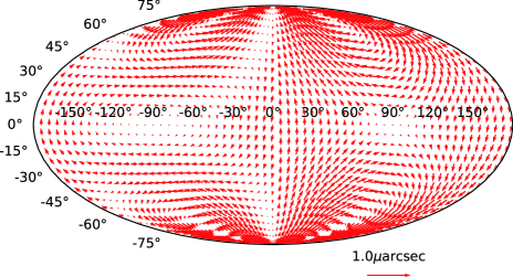
Figure 1: Proper motions obtained from the Gaia data of the SDSS-Gaia QSO sample. The best-fit spherical harmonics for Gaia proper motion measurements are obtained by a calculation of the chi-square method. The red arrows show the vectors of proper motion fields. The length of reference for arrows ($1\,\mu$arcsec) is also shown at the right bottom.

IV Calculations and Results

We acquire proper motions with the SDSS-Gaia QSO sample, and perform fitting the proper motion fields with the spherical harmonics of equation (7) in Section II. We obtain the best-fit spherical harmonics with the typical field strength of $\mathcal{O}(0.1)\,\mu$arcsec that is presented in Figure 1. We estimate $\Omega_{\rm gw}(f)$ from the best-fit spherical harmonics with the equation (8), and obtain the corresponding value $\Omega_{\rm gw}(f)=0.964\times 10^{-4}$. Because the 2 $\sigma$ deviation of the energy density of GWs is $3.804\times 10^{-4}$ (see Appendix B), the constraint becomes $\Omega_{\rm gw}=(0.964\pm 3.804)\times 10^{-4}$ (95 % confidence level (CL)).

This result is consistent with the one of D18 who use VLBI technique, while the sensitivity of the energy density of GWs has been significantly improved by more than one orders of magnitude from D18. By using $\Omega_{\rm gw}(f)<0.4767\times 10^{-3}$ (95 % CL) and equation (10), we derive the upper limit on the strain amplitude $h_{\rm c}(f)<0.868\times 10^{-11}/(f/10^{-9}\,[{\rm Hz}])$.

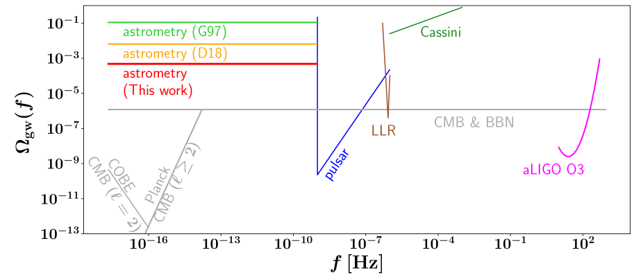
Figure 2: Gaia constraint on the energy density of GWs shown with the red line. From low frequency to high frequency, the pink, dark green, brown, blue, green and orange lines represent the O3 run of the aLIGO (aLIGO O3) [24], Cassini [25], the Lunar laser ranging (LLR) [26, 27], pulsar timing array (pulsar) [28], previous studies (G97, D18). The gray lines represent constraints in the early Universe ($z>1090$) from CMB & BBN [29], CMB at $2\leq\ell\leq 2000$ (Planck) [30], CMB at $\ell=2$ (COBE)[31]

V Discussion

Super massive blackhole binary mergers emit GWs only at the frequency range $f\lesssim 10^{-9}\,[{\rm Hz}]$ because the size of the event horizon is very large. GWs at this range cannot be detected with laser interferometers on the ground such as aLIGO due to the large seismic noise in this frequency range. When we consider an inspiral phase of SMBH binary with the orbital radius $a$, we estimate the amplitude of GWs $h_{\rm expt}$ and the frequency $f_{\rm insp}$ in Matsubayashi et al. (2004) [32], hereafter M04, as

$$f_{\rm insp} = \dfrac{1}{\pi}\sqrt{\dfrac{GM_{\rm T}}{a^{3}}}$$ (16)

$$= 1.14\times 10^{-9}\times\left(\dfrac{a}{100R_{\rm grav}}\right)^{3/2}\left(\dfrac{M_{\rm T}}{10^{10}\,{\rm M}_{\odot}}\right)^{-1}\,,$$

$$h_{\rm expt} = \sqrt{\dfrac{5}{32}}\left(\dfrac{\pi^{2}G^{5}}{c^{12}}\right)^{1/3}\left(\dfrac{f^{2}}{M_{\rm T}}\right)^{1/3}\dfrac{GM_{1}M_{2}}{r}$$

$$= 0.691\times 10^{-11}\times\left(\dfrac{M_{1}}{10^{10}\,{\rm M}_{\odot}}\right)\left(\dfrac{M_{2}}{10^{10}\,{\rm M}_{\odot}}\right)$$

$$\times \left(\dfrac{M_{\rm T}}{2\times 10^{10}\,M_{\odot}}\right)^{-1/3}\left(\dfrac{f}{10^{-9}\,[{\rm Hz}]}\right)^{2/3}\left(\dfrac{r}{400\,[{\rm kpc}]}\right)^{-1}\,$$

where $M_{1}$ and $M_{2}$ are the masses of the primary and secondary SMBHs, respectively. $M_{\rm T}$ is the total mass of the system, which is $M_{\rm T}=M_{1}+M_{2}$. $R_{\rm grav}$ is defined as $R_{\rm grav}=2GM_{\rm T}/c^{2}$. $r$ is the distance of the binary system from the Earth.

We adopt the fiducial values of $M_{1}=M_{2}=10^{10}\,{\rm M}_{\odot}$, $a=100R_{\rm grav}$ and $r=400$ kpc, and find $h_{\rm expt}=0.691\times 10^{-11}$. Because this value of $h_{\rm expt}$ does not meet the upper limit of $h_{\rm c}(f)<0.868\times 10^{-11}/(f/10^{-9}\,[{\rm Hz}])$, we exclude the existence of such SMBH binary systems at $r<400$ kpc from the Earth. One can exclude existence of SMBH binaries with $R=100R_{\rm grav}$ and $M_{\rm T}=2\times 10^{10}\,M_{\odot}$ in the local group.

Our constraint on low frequency GWs is about 100 times weaker than a theoretical forecast (Book & Flanagan 2011 [33]). This difference between our constraint and the expectation is probably produced by the fact that the theoretical forecast only does not include systematic errors, but statistical errors. In the Gaia EDR3 data, the systematic errors become typically 400 $\mu$arcsec/yr at $G=20$, which is 10 times larger than the designed value of Gaia. One can expect that the systematic errors of Gaia will be reduced by improvements from the new multiple visit data and the proper motion model. According to the European Space Agency (ESA), the uncertainty on future releases of Gaia DR5 is expected to be suppressed to 40 $\mu$arcsec/yr at $G=20$. By this improvement, in DR5, one can constrain the existence of low frequency GWs with $\Omega_{\rm gw}\simeq 10^{-6}$ as Book and Flanagan (2011) [33] predict.

We summarize the sensitivity of detection and upper limits of GWs in Figure 2. Figure 2 presents, from the high to low frequencies, aLIGO [24], a planetary exploration spacecraft (Cassini [25]) the lunar laser ranging (LLR) [26, 27], the pulsar timing [28], astrometry of the extragalactic objects (D18, G97 and this work), the abundance of relativistic components which affect the anisotropy of the cosmic microwave background (CMB) and the Big Bang nucleosynthesis (BBN) [29], the quadrupole temperature fluctuation ($\ell=2$) of CMB measured by COBE (COBE) [31], and the CMB angular spectra ($\ell\geq 2$) (Planck) [30]. Although Figure 2 does not include relatively high upper limits above $(\Omega_{\rm gw}(f)\gtrsim 10^{0})$, there exist constraints from a torsion bar detector (TOBA) [34, 35], the global positioning system[36], seismic measurements of the Earth [37], a Lunar orbiter [36] and another planetary exploration spacecraft (ULYSSESS [38]).

As for the future prospects, we expect to obtain the constraint of the energy density of GWs down to $(\Omega_{\rm gw}\sim 10^{-6})$ with the forthcoming Gaia DR5 data as discussed above in this section. This constraint is comparable with the one given by CMB & BBN at $z\gg 1090$, but will be the strongest constraint at $z=0$. Moreover, this constraint is also comparable with the one for this low frequency range of $f[{\rm Hz}]\lesssim 10^{-9}$ expected by the experiment of the Square Kilometre Array (SKA) that will observe $10^{6}$ QSOs every month with the precision $\sim 10\,\mu$arcsec in the VLBI mode. In this way, the DR5 data of the Gaia astrometric satellite will provide the promising constraint at the low fraquency range. With this constraint, one can probe for mergers of SMBH binaries at a distance up to about 4 Mpc, and test the existence of SMBH mergers in the local group.

VI Conclusion

In this paper, we focus on the property of low frequency GWs, which creates apparent proper motions of astronomical objects. Because intrinsic proper motions of QSOs are negligible, we use QSOs for constraining the energy density of low frequency ($\lesssim 10^{-9}\,{\rm Hz}=(30\,{\rm yr})^{-1}$) GWs. We construct the Gaia-SDSS QSO sample with SDSS and Gaia data, cross-matching Gaia EDR3 sources and the SDSS QSOs, where the SDSS QSOs are spectroscopically confirmed. The Gaia-SDSS sample consists of 400,894 with the negligibly small number of contaminating objects only up to $\sim 10$.

We use the Gaia proper motion measurements for the QSOs in the Gaia-SDSS sample. While the astrometric measurement of Gaia is comparable to the one of VLBI, the number of QSOs is $\sim 500$ times larger than that of the VLBI study (D18). We obtain the best-fit spherical harmonics of proper motion of QSOs with the typical field strength of $\mathcal{O}(0.1)\,\mu$arcsec. On the basis of the relation between the proper motion and the energy density of GWs that is described in the equation (8), we obtain the constraint of low frequency GWs ($f<10^{-9}\,[{\rm Hz}]$) that is $\Omega_{\rm gw}=(0.964\pm 3.804)\times 10^{-4}$. By using formulae in M04, we exclude the existence of a SMBH binary within 400 kpc from the Earth including the Milky Way center and the local group with the fiducial setup.

VII Acknowledgements

Numerical computations were carried out on analysis servers and Cray XC50 at the Center for Computational Astrophysics (CfCA), National Astronomical Observatory of Japan, Cray XC40 at the Yukawa Institute Computer Facility in Kyoto University. SA and MS acknowledges the Center for Computational Astrophysics, National Astronomical Observatory of Japan, for providing the computing resources of analysis servers and Cray XC50. This work was supported by the joint research program of the Institute for Cosmic Ray Research (ICRR), University of Tokyo. This paper is supported by World Premier International Research Center Initiative (WPI Initiative), MEXT, Japan, and KAKENHI (20H00180) Grant-in-Aid for Scientific Research (A) through Japan Society for the Promotion of Science. MS is supported by JSPS KAKENHI Grant Nos. JP19K14718 and JP20H05859. DY is supported by JSPS KAKENHI Grant Nos. 17K14304, 19H01891.

VIII Appendix

VIII.1 Mathematical formulae of spherical harmonics

In this section, we show the mathematical formulae of eigenvectors of spherical harmonics. One writes the elements of the eigenvectors of spherical harmonics, $\vec{e}_{\theta}\cdot\vec{Y}^{\rm E}_{\ell m}$, $\vec{e}_{\varphi}\cdot\vec{Y}^{\rm E}_{\ell m}$, $\vec{e}_{\theta}\cdot\vec{Y}^{\rm B}_{\ell m}$ and $\vec{e}_{\varphi}\cdot\vec{Y}^{\rm B}_{\ell m}$ as follows. In the case that $|m|<\ell$, one has

$$\vec{e}_{\theta}\cdot\vec{Y}^{\rm E}_{\ell,m}(\theta,\varphi) = -\dfrac{1}{2}\left[\sqrt{(\ell-m)(\ell+m+1)}e^{-i\varphi}Y_{\ell,m+1}(\theta,\varphi)\right.$$ (18)

$$- \left.\sqrt{(\ell+m)(\ell-m+1)}e^{i\varphi}Y_{\ell,m-1}(\theta,\varphi)\right]\,,$$

$$\vec{e}_{\varphi}\cdot\vec{Y}^{\rm E}_{\ell,m}(\theta,\varphi) = -\dfrac{im}{\sin\theta}Y_{\ell,m}(\theta,\varphi)\,,$$ (19)

$$\vec{e}_{\theta}\cdot\vec{Y}^{\rm B}_{\ell,m}(\theta,\varphi) = \dfrac{im}{\sin\theta}Y_{\ell,m}(\theta,\varphi)\,,$$ (20)

$$\vec{e}_{\varphi}\cdot\vec{Y}^{\rm B}_{\ell,m}(\theta,\varphi) = -\dfrac{1}{2}\left[\sqrt{(\ell-m)(\ell+m+1)}e^{-i\varphi}Y_{\ell,m+1}(\theta,\varphi)\right.$$ (21)

$$- \left.\sqrt{(\ell+m)(\ell-m+1)}e^{i\varphi}Y_{\ell,m-1}(\theta,\varphi)\right]\,.$$

In the case that $m=\ell$, one has

$$\vec{e}_{\theta}\cdot\vec{Y}^{\rm E}_{\ell,m}(\theta,\varphi) = \dfrac{1}{2}\left[\sqrt{(\ell+m)(\ell-m+1)}e^{i\varphi}Y_{\ell,m-1}(\theta,\varphi)\right]\,,$$

$$\vec{e}_{\varphi}\cdot\vec{Y}^{\rm E}_{\ell,m}(\theta,\varphi) = -\dfrac{im}{\sin\theta}Y_{\ell,m}(\theta,\varphi)\,,$$ (23)

$$\vec{e}_{\theta}\cdot\vec{Y}^{\rm B}_{\ell,m}(\theta,\varphi) = \dfrac{im}{\sin\theta}Y_{\ell,m}(\theta,\varphi)\,,$$ (24)

$$\vec{e}_{\varphi}\cdot\vec{Y}^{\rm B}_{\ell,m}(\theta,\varphi) = \dfrac{1}{2}\left[\sqrt{(\ell+m)(\ell-m+1)}e^{i\varphi}Y_{\ell,m-1}(\theta,\varphi)\right]\,$$ (25)

.

In the case that $m=-\ell$, one has

$$\vec{e}_{\theta}\cdot\vec{Y}^{\rm E}_{\ell,m}(\theta,\varphi) = -\dfrac{1}{2}\left[\sqrt{(\ell-m)(\ell+m+1)}e^{-i\varphi}Y_{\ell,m+1}(\theta,\varphi)\right]\,,$$

$$\vec{e}_{\varphi}\cdot\vec{Y}^{\rm E}_{\ell,m}(\theta,\varphi) = -\dfrac{im}{\sin\theta}Y_{\ell,m}(\theta,\varphi)\,,$$ (27)

$$\vec{e}_{\theta}\cdot\vec{Y}^{\rm B}_{\ell,m}(\theta,\varphi) = \dfrac{im}{\sin\theta}Y_{\ell,m}(\theta,\varphi)\,,$$ (28)

$$\vec{e}_{\varphi}\cdot\vec{Y}^{\rm B}_{\ell,m}(\theta,\varphi) = -\dfrac{1}{2}\left[\sqrt{(\ell-m)(\ell+m+1)}e^{-i\varphi}Y_{\ell,m+1}(\theta,\varphi)\right]\,,$$

where $Y_{\ell,m}$ is spherical harmonics, which is the solution of Laplace’s equation. $\vec{Y}^{\rm E}_{\ell,m}$ and $\vec{Y}^{\rm B}_{\ell,m}$ yield

$$\int_{0}^{2\pi}\int_{0}^{\pi}\vec{Y}^{\rm E}_{\ell m}(\theta,\varphi)\cdot\vec{Y}^{\rm E}_{\ell^{\prime}m^{\prime}}(\theta,\varphi)\sin\theta d\theta d\varphi = \delta(\ell,\ell^{\prime})\delta(m,m^{\prime})~{},$$ (30)

$$\int_{0}^{2\pi}\int_{0}^{\pi}\vec{Y}^{\rm B}_{\ell m}(\theta,\varphi)\cdot\vec{Y}^{\rm B}_{\ell^{\prime}m^{\prime}}(\theta,\varphi)\sin\theta d\theta d\varphi = \delta(\ell,\ell^{\prime})\delta(m,m^{\prime})~{},$$ (31)

$$\int_{0}^{2\pi}\int_{0}^{\pi}\vec{Y}^{\rm E}_{\ell m}(\theta,\varphi)\cdot\vec{Y}^{\rm B}_{\ell^{\prime}m^{\prime}}(\theta,\varphi)\sin\theta d\theta d\varphi = 0(\forall\ell,\ell^{\prime},m,m^{\prime}\in\mathbb{Z})~{},$$

where $\delta(i,j)$ is the Kronecker delta such as

$$\delta(i,j)=\begin{cases}1\,\,(i=j)\\ 0\,\,(i\neq j)~{}.\end{cases}$$ (33)

VIII.2 method of an error estimation

In this section, we explain the estimation method of the error of the energy density of the long period GWs. The error is estimated by Fisher matrix method. In this paper, we define the likelihood function $\mathcal{L}$ as

$$-2\ln(\mathcal{L}) = \displaystyle\sum_{k=1}^{N_{\rm sample}}\left\{\dfrac{\left(\mu^{\rm obs}_{\theta,k}-\mu^{\rm th}_{\theta}\right)^{2}}{(\sigma_{\theta,k}^{\rm obs})^{2}}+\dfrac{\left(\mu^{\rm obs}_{\varphi,k}-\mu^{\rm th}_{\varphi}\right)^{2}}{(\sigma_{\varphi,k}^{\rm obs})^{2}}\right\}~{}.$$

The element of Fisher matrix $F$ is

$$F_{X_{i}X_{j}} \equiv \dfrac{d^{2}}{dX_{i}dX_{j}}(-2\ln(\mathcal{L}))$$ (35)

$$= 2\displaystyle\sum_{k=1}^{N_{\rm sample}}\left[\dfrac{1}{(\sigma_{\theta,k}^{\rm obs})^{2}}\dfrac{d\mu_{\theta}^{\rm th}(\theta_{k},\varphi_{k})}{dX_{i}}\dfrac{d\mu_{\theta}^{\rm th}(\theta_{k},\varphi_{k})}{dX_{j}}\right.$$

$$+\left.\dfrac{1}{(\sigma_{\varphi,k}^{\rm obs})^{2}}\dfrac{d\mu_{\varphi}^{\rm th}(\theta_{k},\varphi_{k})}{dX_{i}}\dfrac{d\mu_{\varphi}^{\rm th}(\theta_{k},\varphi_{k})}{dX_{j}}\right]~{}.$$

One sigma deviation of a quantity $X_{i}$, $\sigma(X_{i})$, can be estimated with the inverse matrix of $F$, $F^{-1}$, as

$$\sigma(X_{i})=\sqrt{(F^{-1})_{X_{i}X_{i}}}~{}.$$ (36)

One sigma deviation of $\Omega_{\rm gw}$, $\sigma(\Omega_{\rm gw})$, is

$$\sigma(\Omega_{\rm gw}) = \dfrac{3}{2\pi\tilde{H}_{0}^{2}}\left\{\left[(E_{2,0})\sigma(E_{2,0})\right]^{2}\right.+\left[(B_{2,0})\sigma(E_{2,0})\right]^{2}$$ (37)

$$+\displaystyle\sum_{m=1}^{2}\left(\left[2{\rm Re}(E_{2,m})\sigma(E_{2,m})\right]^{2}\right.$$

$$+\left[{\rm Im}(E_{2,m})\sigma(E_{2,m})\right]^{2}$$

$$+\left[{\rm Re}(B_{2,m})\sigma(B_{2,m})\right]^{2}$$

$$+\left[{\rm Im}(B_{2,m})\sigma(B_{2,m})\right]^{2}{\Large{\text{)}}}{\Large{\text{\}}}}^{1/2}~{}.$$

In order to obtain 95 % CL of the energy density of GWs, we show $\Omega_{\rm gw}\pm 2\sigma(\Omega_{\rm gw})$ as the constraint.

References

- [1] B. P. Abbott et al. Phys. Rev. Lett. 116 (Feb., 2016) 061102 [1602.03837].
- [2] B. P. Abbott et al. ApJ 848 (Oct., 2017) L13 [1710.05834].
- [3] D. Langlois et al. Phys. Rev. D 97 (Mar., 2018) 061501 [1711.07403].
- [4] S. Peirone et al. Phys. Rev. D 100 (Sept., 2019) 063509 [1905.11364].
- [5] C. Deffayet, G. Esposito-Farèse, A. Vikman Phys. Rev. D 79 (Apr., 2009) 084003 [0901.1314].
- [6] M. Roos, Introduction to cosmology. 2003.
- [7] B. P. Abbott et al. Nature 551 (Nov., 2017) 85–88 [1710.05835].
- [8] K. Hotokezaka et al. Nature Astronomy 3 (July, 2019) 940–944 [1806.10596].
- [9] B. F. Schutz Nature 323 (Sept., 1986) 310–311.
- [10] C. R. Gwinn et al. ApJ 485 (Aug., 1997) 87–91 [astro-ph/9610086].
- [11] J. Darling, A. E. Truebenbach, J. Paine ApJ 861 (July, 2018) 113 [1804.06986].
- [12] Gaia Collaboration et al. A&A 595 (Nov., 2016) A1 [1609.04153].
- [13] Gaia Collaboration et al. arXiv e-prints (Dec., 2020) arXiv:2012.01533 [2012.01533].
- [14] L. Lindegren et al. arXiv e-prints (Dec., 2020) arXiv:2012.03380 [2012.03380].
- [15] M. Crosta, M. G. Lattanzi, A. Spagna Baltic Astronomy 8 (Jan., 1999) 239–251.
- [16] C. J. Moore et al. Phys. Rev. Lett. 119 (Dec., 2017) 261102 [1707.06239].
- [17] S. A. Klioner Classical and Quantum Gravity 35 (Feb., 2018) 045005 [1710.11474].
- [18] Y. Wang et al. arXiv e-prints (Oct., 2020) arXiv:2010.02218 [2010.02218].
- [19] F. Mignard, S. Klioner A&A 547 (Nov., 2012) A59 [1207.0025].
- [20] Strictly speaking, GWs creates multipole modes (see [30]). However, because the quadruple mode () is dominated in the generated proper motions with low frequency GWs, we only focus on the quadruple mode of proper motions.
- [21] Planck Collaboration et al. A&A 641 (Sept., 2020) A6 [1807.06209].
- [22] D. Sivia, J. Skilling, Data Analysis: A Bayesian Tutorial. OUP Oxford, 2006.
- [23] The KD-tree method enables to cross-match the objects with the cost for each object. Here is the size of the sample.
- [24] B. P. Abbott et al. Phys. Rev. Lett. 120 (Mar., 2018) 091101 [1710.05837].
- [25] J. W. Armstrong et al. ApJ 599 (Dec., 2003) 806–813.
- [26] B. Mashhoon, B. J. Carr, B. L. Hu ApJ 246 (June, 1981) 569–591.
- [27] L. Biskupek, J. Müller, J.-M. Torre Universe 7 (Feb., 2021) 34 [2012.12032].
- [28] P. D. Lasky et al. Physical Review X 6 (Jan., 2016) 011035 [1511.05994].
- [29] L. Pagano, L. Salvati, A. Melchiorri Physics Letters B 760 (Sept., 2016) 823–825 [1508.02393].
- [30] T. Namikawa et al. Phys. Rev. D 100 (July, 2019) 021303 [1904.02115].
- [31] M. Maggiore Phys. Rep. 331 (July, 2000) 283–367 [gr-qc/9909001].
- [32] T. Matsubayashi, H.-a. Shinkai, T. Ebisuzaki ApJ 614 (Oct., 2004) 864–868.
- [33] L. G. Book, É. É. Flanagan Phys. Rev. D 83 (Jan., 2011) 024024 [1009.4192].
- [34] K. Ishidoshiro et al. Phys. Rev. Lett. 106 (Apr., 2011) 161101 [1103.0346].
- [35] T. Shimoda et al. arXiv e-prints (Dec., 2018) arXiv:1812.01835 [1812.01835].
- [36] S. Aoyama, R. Tazai, K. Ichiki Phys. Rev. D 89 (Mar., 2014) 067101 [1402.4521].
- [37] M. Coughlin, J. Harms Phys. Rev. Lett. 112 (Mar., 2014) 101102 [1401.3028].
- [38] B. Bertotti et al. A&A 296 (Apr., 1995) 13.