Knapsack and Subset Sum with Small Items

Abstract

Knapsack and Subset Sum are fundamental NP-hard problems in combinatorial optimization. Recently there has been a growing interest in understanding the best possible pseudopolynomial running times for these problems with respect to various parameters.

In this paper we focus on the maximum item size $s$ and the maximum item value $v$. We give algorithms that run in time $\mathcal{O}(n+s^{3})$ and $\mathcal{O}(n+v^{3})$ for the Knapsack problem, and in time $\widetilde{\mathcal{O}}(n+s^{5/3})$ for the Subset Sum problem.

Our algorithms work for the more general problem variants with multiplicities, where each input item comes with a (binary encoded) multiplicity, which succinctly describes how many times the item appears in the instance. In these variants $n$ denotes the (possibly much smaller) number of distinct items.

Our results follow from combining and optimizing several diverse lines of research, notably proximity arguments for integer programming due to Eisenbrand and Weismantel (TALG 2019), fast structured $(\min,+)$-convolution by Kellerer and Pferschy (J. Comb. Optim. 2004), and additive combinatorics methods originating from Galil and Margalit (SICOMP 1991).

1 Introduction

In the Knapsack problem we are given a (multi-)set consisting of $N$ items, where the $i$-th item has size $s_{i}$ and value $v_{i}$, and a knapsack capacity $t$. The task is to find a subset of items with the maximum total value such that its total size does not exceed the capacity $t$. In the related Subset Sum problem we are given a (multi-)set of $N$ positive integers and a target value $t$, and the task is to find a subset of integers with the total sum exactly equal to $t$. The Subset Sum problem can thus be seen as a decision variant of the Knapsack problem with the additional restriction that $s_{i}=v_{i}$ for every item $i$.

Knapsack and Subset Sum are fundamental problems in computer science and discrete optimization. They are studied extensively both from practical and theoretical points of view (see, e.g. [23] for a comprehensive monograph). The two problems are (weakly) NP-hard, and Bellman’s seminal work on dynamic programming [7] gives pseudopolynomial $\mathcal{O}(Nt)$ time algorithms for both of them. Recently there has been a growing interest in understanding the best possible pseudopolynomial running times for these problems with respect to various parameters, see, e.g., [9, 6, 16, 5, 11].

In this paper we consider binary multiplicity encoding of the Knapsack and Subset Sum instances. Each item $i$ given in the input has a (binary encoded) positive integer multiplicity $u_{i}$, which denotes that up to $u_{i}$ copies of this item can be used in a solution. In these variants $n$ denotes the (possibly much smaller) number of distinct items and $N=\sum_{i\in[n]}u_{i}$. Binary multiplicity encoding can be challenging because one requires the algorithm to run in polynomial time in the input size, which can be exponentially smaller compared to the naive encoding. A notable example of this setting is the breakthrough result of Goemans and Rothvoß [18] showing that Bin Packing with few different item sizes (and binary multiplicity encoding) can be solved in polynomial time.

Formally, Knapsack with multiplicities can be defined as an integer linear program: maximize $\sum_{i\in[n]}v_{i}x_{i}$ subject to $0\leqslant x_{i}\leqslant u_{i}$, $x_{i}\in\mathbb{Z}$, and $\sum_{i\in[n]}s_{i}x_{i}\leqslant t$. Similarly, Subset Sum with multiplicities can be defined as a feasibility integer linear program with constraints $0\leqslant x_{i}\leqslant u_{i}$, $x_{i}\in\mathbb{Z}$, and $\sum_{i\in[n]}s_{i}x_{i}=t$. Throughout the paper we use $u$ to denote the maximum item multiplicity $\max_{i\in[n]}u_{i}$, and w.l.o.g. we assume that $u\leqslant t$.

1.1 Our results

We focus on pseudo-polynomial time algorithms with respect to the maximum item size $s=\max_{i\in[n]}s_{i}$ (or maximum item value $v=\max_{i\in[n]}v_{i}$, which is essentially equivalent). We note that $s$ is a stronger parameter compared to $t$ in the sense that $s$ can be much smaller than $t$, but not vice versa. Yet, $s$ is less well understood than $t$. In the regime where $n$ is large compared to $s$, an $\mathcal{O}(n+\mathrm{poly}(s))$ time algorithm would be desirable. We show that the Knapsack problem can indeed be solved in such a time. Prior results (even for 0-1 Knapsack, that is, without multiplicities) only came with the form $\mathcal{O}(\mathrm{poly}(n)\cdot\mathrm{poly}(s))$ or $\mathcal{O}(\mathrm{poly}(s)\cdot\mathrm{poly}(t))$.

This raises the natural question what the best exponent in the polynomial is. In this paper we address the question from the upper bound side. We give algorithms for Knapsack running in $\mathcal{O}(n+s^{3})$ and $\mathcal{O}(n+v^{3})$ time, and for Subset Sum running in $\widetilde{\mathcal{O}}(n+s^{5/3})$ time. Our algorithms are in the word RAM model, and we assume that each integer in the input fits in one word. In particular, arithmetic operations on integers of size polynomial in the sum of the input’s integers require constant time.

Our first result is an algorithm for Knapsack. We use proximity techniques due to Eisenbrand and Weismantel [16] which allow us to prove that there is an efficiently computable solution that differs only very little from an optimal solution. Then we apply a fast algorithm for structured $(\min,+)$-convolution [22] to search for this optimal solution within the limited space. This results in a running time which is cubic in the maximum item size.

Theorem 1.1.

Knapsack (with multiplicities) can be solved in deterministic $\mathcal{O}(n+s^{3})$ time.

The definition of (the decision variant of) the Knapsack problem is symmetric with respect to sizes and values. We give a simple transformation that allows us to apply our algorithm also to the case where the maximal item value (and not the maximal item size) is small.

Theorem 1.2.

Knapsack (with multiplicities) can be solved in deterministic $\mathcal{O}(n+v^{3})$ time.

Theorem 1.1 already implies that Subset Sum can also be solved in $\mathcal{O}(n+s^{3})$. Our algorithm uses as a subprocedure an $\mathcal{O}(n+st)$ time Knapsack algorithm (see Lemma 2.3). If we simply replaced it with a $\widetilde{\mathcal{O}}(N+t)$ time algorithm for Subset Sum [9], we would get a $\widetilde{\mathcal{O}}(n+s^{2})$ time algorithm for Subset Sum. We improve on this by introducing a refined proximity argument that lets us further reduce an instance, where the maximum item multiplicity $u$ can be of the order of $s$, to two instances with $u\ll s$ each. By combining this with additive combinatorics methods, originally developed by Galil and Margalit [17] and recently generalized by Bringmann and Wellnitz [11], we then obtain a subquadratic algorithm.

Theorem 1.3.

Subset Sum (with multiplicities) can be solved in randomized $\widetilde{\mathcal{O}}(n+s^{5/3})$ time, with a one-sided error algorithm that returns a correct answer with high probability.

All our algorithms can also retrieve a solution, without increasing the asymptotic running times. This is notable especially for our Subset Sum algorithm, in which we use as a black box the Bringmann-Wellnitz algorithm that gives only yes/no answers. We can deal with this presumable obstacle because we can afford to spend more time on retrieving a solution than the Bringmann-Wellnitz algorithm could.

A limitation of our algorithms is that they can provide an answer only for a single target value $t$ at a time. Conversely, many (but not all) known Knapsack and Subset Sum algorithms can give answers for all target values between $0$ and $t$ at the same time. This limitation is however unavoidable: We aim at running times independent of the target value $t$, thus we cannot afford output size linear in $t$, because $t$ cannot be bounded in terms of $n$ and $s$ only.

In the next section we discuss how our results fit a broader landscape of existing Knapsack and Subset Sum algorithms.

1.2 Related work

Pseudopolynomial time algorithms for Knapsack

Bellman [7] was the first to show that the Knapsack problem admits a pseudopolynomial time algorithm. He presented an $\mathcal{O}(Nt)$ time algorithm based on dynamic programming. Pisinger [28] gave an $\mathcal{O}(Nsv)$ time algorithm, which is an improvement for instances with both small sizes and small values. He proved that only balanced feasible solutions to Knapsack need to be considered in order to find an optimal solution. Then he used this observation to decrease the number of states of the dynamic program. His arguments may be thought of as an early example of proximity-based arguments.

Kellerer and Pferschy [22] studied approximation algorithms for Knapsack. As a subroutine they developed a $\widetilde{\mathcal{O}}(N+vp)$ time (exact) algorithm, where $p$ denotes the optimal total value. Their algorithm can be easily modified to work in $\widetilde{\mathcal{O}}(N+st)$ time. Their approach, based on fast $(\min,+)$-convolution for structured (convex) instances was rediscovered and improved by Axiotis and Tzamos [5]. Bateni et al. [6] achieved the same $\widetilde{\mathcal{O}}(N+st)$ running time with a different method, which can be seen as a far-reaching refinement of Pisinger’s idea [28]. They also developed the prediction technique, which let them achieve $\widetilde{\mathcal{O}}(N+vt)$ running time.

Eisenbrand and Weismantel [16] studied more general integer linear programs, and presented a $\widetilde{\mathcal{O}}(ns^{2})$ time algorithm for Knapsack with multiplicities, based on proximity-based arguments. To the best of our knowledge they are the first to consider Knapsack with multiplicities. Subsequently Axiotis and Tzamos [5] improved logarithmic factors (in the non-multiplicity setting) and gave an $\mathcal{O}(Ns^{2})$ time algorithm, which they also generalized to $\mathcal{O}(Nv^{2})$ time. Bateni et al. [6] also explicitly consider the Knapsack problem with multiplicities and independently designed a $\widetilde{\mathcal{O}}(ns^{2}\min\{n,s\})$ time algorithm.

Axiotis and Tzamos suggested [5, Footnote 2] that the fast convex convolution can be combined with proximity-based arguments of Eisenbrand and Weismantel [16] to obtain an algorithm for small items with running time independent of $t$. However, a direct application of Eisenbrand and Weismantel [16] proximity argument (see [16, Section 4.1]) reduces an instance to $t\leqslant\mathcal{O}(ns^{2})$, which, in combination with $\mathcal{O}(N+st)$ algorithm, yields $\mathcal{O}(N+ns^{3})$ runtime. Our algorithm improves it to $\mathcal{O}(n+s^{3})$ by a more careful proximity argument and a convex convolution that explicitly handles negative items. Moreover, we show how to extend this reasoning to the multiplicity setting.

Remark 1.4.

Lawler [26] showed that the variant with multiplicities can be reduced to the 0-1 variant. His reduction transforms a multiset composed of at most $u$ copies of each of $n$ distinct numbers bounded by $s$ into an instance of $\mathcal{O}(n\log{u})$ numbers bounded by $\mathcal{O}(us)$. This easily enables us to adapt algorithms with no time dependence on $s$ (e.g., the $\mathcal{O}(Nt)$ time algorithm of Bellman) into the setting with multiplicities (with logarithmic overhead).

Remark 1.5.

There is also a folklore reduction that enables us to bound $N\leqslant\widetilde{\mathcal{O}}(t)$ for the variant with multiplicities. For each $x\in[s]$ keep $\left\lfloor t/x\right\rfloor$ most profitable items of size $s_{i}=x$. This leaves us with at most $N\leqslant\mathcal{O}(t\log(t))$ items and does not increase the item sizes.

See Table 1 for a summary of the known results for Knapsack.

Table 1: Pseudopolynomial time algorithms for Knapsack. $N$ is the total number of items, $n$ is the number of distinct items, $t$ is the knapsack capacity, $s$ is the maximum size and $v$ the maximum value of an item. Symbol (–) means that no non-trivial optimization is given for the respective regime; running times can still be derived from the trivial inequalities $n\leqslant N$ and $t\leqslant Ns$. We use symbol $(\ddagger)$ when Remark 1.4 applies and $(\dagger)$ when Remark 1.5 applies.

0-1 Knapsack	with multiplicities	Reference
$\mathcal{O}(Nt)$	$\widetilde{\mathcal{O}}(nt)^{\ddagger}$	Bellman [7]
$\mathcal{O}(Nsv)$	–	Pisinger [28]
$\widetilde{\mathcal{O}}(N+st)$	$\widetilde{\mathcal{O}}(n+st)^{\dagger}$	Kellerer and Pferschy [22], also [6, 5]
$\widetilde{\mathcal{O}}(N+vt)$	$\widetilde{\mathcal{O}}(n+vt)^{\dagger}$	Bateni et al. [6]
–	$\widetilde{\mathcal{O}}(ns^{2}\min\{n,s\})$	Bateni et al. [6]
$\mathcal{O}(N\min\{s^{2},v^{2}\})$	–	Axiotis and Tzamos [5]
–	$\widetilde{\mathcal{O}}(ns^{2})$	Eisenbrand and Weismantel [16]
–	$\mathcal{O}(n+\min\{s^{3},v^{3}\})$	This paper

Pseudopolynomial time algorithms for Subset Sum

Subset Sum is a special case of Knapsack and we expect significantly faster algorithms for it. Pisinger’s algorithm [28] runs in $\mathcal{O}(Ns)$ time for Subset Sum. The first improvement in all parameter regimes over the $\mathcal{O}(Nt)$ time algorithm of Bellman was given by Koiliaris and Xu [24]. They presented $\widetilde{\mathcal{O}}(\sqrt{N}t+N)$, $\widetilde{\mathcal{O}}(N+t^{5/4})$ and $\widetilde{\mathcal{O}}(\Sigma)$ time deterministic algorithms for Subset Sum, where $\Sigma$ is the total sum of items. A by now standard method, used by all these algorithms, is to encode an instance of Subset Sum as a convolution problem that can be solved using Fast Fourier Transform. Subsequently, Bringmann [9] presented a $\widetilde{\mathcal{O}}(N+t)$ randomized time algorithm for Subset Sum based on the color-coding technique. Jin and Wu [21] later gave an alternative $\widetilde{\mathcal{O}}(N+t)$ randomized time algorithm based on Newton’s iterative method. Their proof is notable for being very compact.

From a different perspective, Galil and Margalit [17] used additive combinatorics methods to prove that Subset Sum can be solved in near linear time when $t\gg\Sigma s/N^{2}$ and all items are distinct. Very recently Bringmann and Wellnitz [11] generalized that result to multisets. Their algorithm combined with the $\widetilde{\mathcal{O}}(N+t)$ time algorithm [9] yields a $\widetilde{\mathcal{O}}(N+u^{1/2}s^{3/2})$ time algorithm for Subset Sum with multiplicities (cf., Lemma 2.6). For $u=1$ this gives the currently fastest $\widetilde{\mathcal{O}}(N+s^{3/2})$ time algorithm (in terms of small $s$). With our $\widetilde{\mathcal{O}}(n+s^{5/3})$ time algorithm we improve upon their result for $u\gg s^{1/3}$. We note that even with the naive (not binary) multiplicity encoding our improvement is nontrivial, since the mentioned case with $u=1$ requires that each item has a different size. For example, even an $\mathcal{O}(N+s^{1.99})$ time algorithm does not follow immediately from [9] when multiple items can have the same size. We discuss their additive combinatorics methods in more detail in Section 5.2.

See Table 2 for a summary of the known results for Subset Sum.

Table 2: Pseudopolynomial time algorithms for Subset Sum. $N$ is the total number of items, $n$ is the number of distinct items, $t$ is the target value, $\Sigma$ is the sum of all items, $s$ is the maximum item, and $u$ is the maximum multiplicity of an item. Symbol (–) means that no non-trivial optimization is given for the respective regime; running times can still be derived from the trivial inequalities $n\leqslant N\leqslant nu$ and $t\leqslant Ns$. In $(\star)$ the instance cannot have two items with the same size, the algorithm works only for $u=1$. We use symbol $(\ddagger)$ when Remark 1.4 applies.

0-1 Subset Sum	with Multiplicities	Reference
$\mathcal{O}(Nt)$	$\widetilde{\mathcal{O}}(nt)^{\ddagger}$	Bellman [7]
$\mathcal{O}(Ns)$	–	Pisinger [28]
$\widetilde{\mathcal{O}}(N+\sqrt{N}t)$	$\widetilde{\mathcal{O}}(n+\sqrt{n}t)^{\ddagger}$	Koiliaris and Xu [24]
$\widetilde{\mathcal{O}}(N+t^{5/4})$	$\widetilde{\mathcal{O}}(n+t^{5/4})^{\ddagger}$	Koiliaris and Xu [24]
$\widetilde{\mathcal{O}}(\Sigma)$	–	Koiliaris and Xu [24]
$\widetilde{\mathcal{O}}(N+t)$	$\widetilde{\mathcal{O}}(n+t)^{\ddagger}$	Bringmann [9]
$\widetilde{\mathcal{O}}(N+s^{3/2})$ $\star$	(not applicable)	Galil and Margalit [17]
–	$\widetilde{\mathcal{O}}(N+u^{1/2}s^{3/2})$	Bringmann and Wellnitz [11]
–	$\widetilde{\mathcal{O}}(n+s^{5/3})$	This Paper

Lower bounds

Bringmann’s Subset Sum algorithm [9], which runs in time $\widetilde{\mathcal{O}}(N+t)$, was shown to be near-optimal by using the modern toolset of fine-grained complexity. More precisely, any $t^{1-\varepsilon}2^{o(N)}$ algorithm for Subset Sum, for any $\varepsilon>0$, would violate both the Strong Exponential Time Hypothesis [1] and the Set Cover Conjecture [14]. This essentially settles the complexity of the problem in the parameters $N$ and $t$. These lower bounds use reductions that produce instances with $t=\widetilde{\Theta}(s)$, and therefore they do not exclude a possibility of a $\widetilde{\mathcal{O}}(N+s)$ time algorithm for Subset Sum. The question if such an algorithm exists is still a major open problem [4].

Bringmann and Wellnitz [11] excluded a possibility of a near-linear algorithm for Subset Sum in a dense regime. More precisely, they showed that, unless the Strong Exponential Time Hypothesis and the Strong $k$-Sum Hypothesis both fail, Subset Sum requires $(s\Sigma/(Nt))^{1-o(1)}$ time (where $\Sigma$ is the total sum of items).

For the Knapsack problem Bellman’s algorithm [7] remains optimal for the most natural parametrization by $N$ and $t$. This was explained by Cygan at el. [15] and Künnemann et al. [25], who proved an $(N+t)^{2-o(1)}$ lower bound assuming the $(\min,+)$-Convolution Conjecture. Their hardness constructions create instances of 0-1 Knapsack where $s$ and $t$ are $\widetilde{\Theta}(N)$. This is also the best lower bound known for Knapsack with multiplicities. In particular, an $\mathcal{O}(N+s^{2-\varepsilon})$ time algorithm is unlikely, and our $\mathcal{O}(n+s^{3})$ upper bound leaves the gap for the best exponent between $2$ and $3$.

Other variants of Knapsack and Subset Sum

We now briefly overview other variants of Knapsack and Subset Sum, which are not directly related to our results. The Unbounded Knapsack problem is the special case with $u_{i}=\infty$, for all $i\in[n]$, and one can assume w.l.o.g. $N=n\leqslant s$. For that variant Tamir [31] presented an $\mathcal{O}(n^{2}s^{2})$ time algorithm. Eisenbrand and Weismantel [16] improved this result and gave an $\mathcal{O}(ns^{2})$ time algorithm using proximity arguments. Bateni et al. [6] presented a $\widetilde{\mathcal{O}}(ns+s^{2}\min\{n,s\})$ time algorithm. Then, an $\mathcal{O}(n+\min\{s^{2},v^{2}\})$ algorithm for Unbounded Knapsack was given independently by Axiotis and Tzamos [5] and Jansen and Rohwedder [19]. Finally, Chan and He [13] gave a $\widetilde{\mathcal{O}}(ns)$ time algorithm. Unbounded Knapsack seems to be an easier problem than 0-1 Knapsack because algorithms do not need to keep track of which items are already used in partial solutions. Most of the Unbounded Knapsack techniques do not apply to 0-1 Knapsack.

In the polynomial space setting, Lokshtanov and Nederlof [27] presented a $\widetilde{\mathcal{O}}(N^{4}sv)$ time algorithm for Knapsack and a $\widetilde{\mathcal{O}}(N^{3}t)$ time algorithm for Subset Sum. The latter was subsequently improved by Bringmann [9], who gave a $\widetilde{\mathcal{O}}(Nt^{1+\varepsilon)})$ time and $\widetilde{\mathcal{O}}(N\log{t})$ space algorithm. Recently, Jin, Vyas and Williams [20] presented a $\widetilde{\mathcal{O}}(Nt)$ time and $\widetilde{\mathcal{O}}(\log(Nt))$ space algorithm (assuming a read-only access to $\widetilde{\mathcal{O}}(\log{N}\log{\log{N}}+\log{t})$ random bits).

In the Modular Subset Sum problem, all subset sums are taken over a finite cyclic group $\mathbb{Z}_{m}$, for some given integer $m$. Koiliaris and Xu [24] gave a $\widetilde{\mathcal{O}}(m^{5/4})$ time algorithm for this problem, which was later improved by [4] to $\mathcal{O}(m\log^{7}{m})$. Axiotis et al. [3] independently with Cardinal and Iacono [12] simplified their algorithm and gave an $\mathcal{O}(m\log{m})$ time randomized and $\mathcal{O}(m\,\mathrm{polylog}(m))$ deterministic time algorithms. Recently, Potępa [29] gave the currently fastest $\mathcal{O}(m\log(m)\alpha(m))$ deterministic algorithm for Modular Subset Sum (where $\alpha(m)$ is the inverse Ackerman function).

Bringmann and Nakos [10] designed a near-linear time algorithm for output sensitive Subset Sum by using additive combinatorics methods. Finally, Jansen and Rohwedder [19] considered the Unbounded Subset Sum problem and presented a $\widetilde{\mathcal{O}}(s)$ time algorithm.

2 Techniques

In this section we recall several known techniques from different fields, which we later combine as black boxes in order to get efficient algorithms in the setting with binary encoded multiplicities. We do not expect the reader to be familiar with all of them, and we include their brief descriptions for completeness. Nevertheless, it should be possible to skip reading this section and still get a high-level understanding of our results.

2.1 Proximity arguments

Now we introduce proximity arguments, which will allow us to avoid a dependency on the multiplicities $u_{i}$ in the running time. Very similar arguments were used by Eisenbrand and Weismantel [16] for more general integer linear programs. We reprove them for our simpler case to make the paper self-contained.

We will show that we can efficiently compute a solution to Knapsack which differs from an optimal solution only in a few items. To this end, we define a maximal prefix solution to be a solution obtained as follows. We order the items by their efficiency, i.e. by the ratios $v_{i}/s_{i}$, breaking ties arbitrarily. Then, beginning with the most efficient item, we select items in the decreasing order of efficiency until the point when adding the next item would exceed the knapsack’s capacity. At this point we stop and return the solution.

Note that a maximal prefix solution can be found in time $\mathcal{O}(n)$: We first select the median of $v_{i}/s_{i}$ in time $\mathcal{O}(n)$ [8]. Then, we check if the sum of all the items that are more efficient than the median exceeds $t$. If so, we know that none of the other items are used in the maximal prefix solution. Otherwise, all the more efficient items are used. In both cases we can recurse on the remaining $n/2$ items. The running time is then of the form of a geometric sequence that converges to $\mathcal{O}(n)$.

Lemma 2.1 (cf., [16]).

Let $p$ be a maximal prefix solution to Knapsack. There is an optimal solution $z$ that satisfies $\lVert z-p\rVert_{1}\leqslant 2s$, where $\lVert z-p\rVert_{1}$ denotes $\sum_{i\in[n]}|z_{i}-p_{i}|$.

Proof 2.2.

Let $z$ be an optimal solution which minimizes $\lVert z-p\rVert_{1}$. If all the items fit into the knapsack, $p$ and $z$ must be equal. Otherwise, we can assume that the total sizes of both solutions, i.e. $\sum_{i\in[n]}s_{i}z_{i}$ and $\sum_{i\in[n]}s_{i}p_{i}$, are both between $t-s+1$ and $t$. In particular, we have that

$$-s<\sum_{i\in[n]}s_{i}(p_{i}-z_{i})<s.$$ (1)

For the sake of the proof consider the following process. We start with the vector $z-p$, and we move its components towards zeros, carefully maintaining the bounds of (1). That is, in each step of the process, if the current sum of item sizes is positive, we reduce a positive component by $1$; if the sum is negative, we increase a negative component by $1$. The crucial idea is that during this process in no two steps we can have the same sum of item sizes. Otherwise, one could apply to $z$ the additions and removals performed between the two steps, and therefore obtain another solution that is closer to $p$ and is still optimal. Indeed, the optimiality follows from the fact that this operation does not increase the total size of the solution, and it also cannot decrease the value of the solution, because every item selected by $p$ but not by $z$ has efficiency no lower than every item selected by $z$ but not by $p$. Hence, the number of steps, i.e., $\lVert z-p\rVert_{1}$, is bounded by $2s$.

This lemma can be used to avoid the dependency on multiplicities $u_{1},u_{2},\dotsc,u_{n}$ as follows. We compute a maximal prefix solution $p$. Then we know that there is an optimal solution $z$ with

$$z_{i}\in\{0,\dotsc,u_{i}\}\cap\{p_{i}-2s,\dotsc,p_{i}+2s\}\quad\forall i\in[n].$$

Hence, we can obtain an equivalent instance by fixing the choice of some items. Formally, we remove $\max\{0,p_{i}-2s\}$ many copies of item $i$ and subtract their total size from $t$. If some item still has more than $4s$ copies, we can safely remove the excess. This shows that one can reduce a general knapsack instance to an instance with $u_{i}\leqslant 4s$ for all $i\in[n]$. In particular, a naive application of Bellman’s algorithm would run in time $\mathcal{O}(t\cdot\sum_{i=1}^{n}u_{i})\leqslant\mathcal{O}(n^{2}s^{3})$. Later in this paper we will apply the same proximity statement in more involved arguments.

2.2 Fast structured $(\min,+)$-convolution

Another technique that we use in this paper is a fast algorithm for structured instances of the $(\min,+)$-convolution problem. This technique was already applied in several algorithms for Knapsack [22, 6, 5]. We use it to find solutions for all knapsack capacities in $\{0,\dotsc,t\}$ in time $\mathcal{O}(n+st+t\log^{2}(t))$. We consider a slightly more general variant, where the values of items may also be negative and the knapsack constraint has to be satisfied with equality. To avoid confusion, we let $\bar{v}_{i}\in\mathbb{Z}$, $i\in[n]$, denote these possibly negative values of items.

Lemma 2.3.

Let $\bar{v}_{1},\bar{v}_{2},\dotsc,\bar{v}_{n}\in\mathbb{Z}$. In time $\mathcal{O}(n+st+t\log^{2}(t))$ one can solve

$$\max_{x\in\mathbb{Z}^{n}}\sum_{i\in[n]}\bar{v}_{i}x_{i} \text{ subject to }\sum_{i\in[n]}s_{i}x_{i}=t^{\prime} \text{ and }\quad\forall_{i\in[n]}\ 0\leqslant x_{i}\leqslant u_{i},$$ (2)

for all $t^{\prime}\in\{0,\dotsc,t\}$.

Proof 2.4.

For $h\in[s+1]$ let $w^{(<h)}=\langle w^{(<h)}_{0},w^{(<h)}_{1},\dotsc,w^{(<h)}_{t}\rangle$ where $w^{(<h)}_{t^{\prime}}$ denotes the value of an optimal solution to (2) for the knapsack capacity $t^{\prime}$ when restricting the instance to items $i$ with $s_{i}<h$. If there is no solution satisfying the equality constraint with $t^{\prime}$, we let $w^{(<h)}_{t^{\prime}}=-\infty$. Our goal is to compute the vectors $w^{(<1)},w^{(<2)},\dotsc,w^{(<h+1)}$ iteratively. We define the vector $w^{(h)}=\langle w^{(h)}_{0},w^{(h)}_{1},\dotsc,w^{(h)}_{t}\rangle$ which describes the optimal solutions solely of items $j$ with $s_{j}=h$. For each $i$, the component $w^{(h)}_{t^{\prime}}$ for $t^{\prime}=ih$ is equal to the total value of the $i$ most valuable items of size $h$, or to $-\infty$ if there are less than $i$ items of size $h$. All components for indices not divisible by $h$ are $-\infty$.

Hence, to compute $w^{(h)}$ it suffices to find the $\left\lceil t/h\right\rceil$ most valuable items of size $h$ in the decreasing order of values. In time $\mathcal{O}(n+s)$ we partition the items by their size $s_{i}$. Extracting the $t/h$ most valuable items for all $h\in[s]$ requires in total a time of $\mathcal{O}(n+\sum_{h\in[s]}t/h)\leqslant\mathcal{O}(n+t\log(t))$. Finally, sorting all sets takes in total $\mathcal{O}(\sum_{h\in[s]}t/h\cdot\log(t/h))\leqslant\mathcal{O}(t\log^{2}(t))$ time.

Given $w^{(<h)}$ for some $h$ we want to compute the vector $w^{(<h+1)}$ in time $\mathcal{O}(t)$. Then the lemma follows by iteratively applying this step. To this end we notice that $w^{(<h+1)}$ is precisely the $(\max,+)$-convolution of $w^{(h)}$ and $w^{(<h)}$, that is,

$$w^{(<h+1)}_{i}=\max\left\{w^{(h)}_{j}+w^{(<h)}_{i-j}\mid j\in\{0,\dotsc,i\}\right\}.$$

While in general computing a $(\max,+)$-convolution is conjectured to require quadratic time [15, 25], in this case it can be done efficiently by exploiting the simple structure of $w^{(h)}$. For each remainder $r\in\{0,\dotsc,h-1\}$ we separately compute the entries of indices that are equal to $r$ modulo $h$. We define the matrix $M\in\mathbb{Z}^{\lceil t/h\rceil\times\lceil t/h\rceil}$ with

$$M[i,j]=w^{(<h)}_{jh+r}+w^{(h)}_{(i-j)h},$$

where $w^{(h)}_{(i-j)h}=-\infty$ if $j>i$. We do not explicitly construct the matrix, but we can compute any entry of $M$ in the constant time. To produce the vector $w^{(<h+1)}$ it suffices to find the maximum of each row of $M$. This can be done efficiently, since $M$ is inverse-Monge, that is,

$$M[i,j]+M[i+1,j+1]=w^{(<h)}_{jh+r}+w^{(h)}_{(i-j)h}+w^{(<h)}_{jh+h+r}+w^{(h)}_{(i-j)h}\\ \geqslant w^{(<h)}_{jh+r}+w^{(h)}_{(i-j)h+h}+w^{(<h)}_{jh+h+r}+w^{(h)}_{(i-j)h-h}=M[i+1,j]+M[i,j+1].$$

Therefore, we can compute the row maxima in time $\mathcal{O}(t/h)$ with SMAWK algorithm [2]. This implies a total running time of $\mathcal{O}(t)$ for all remainders $r$ and proves the lemma.

2.3 Additive combinatorics

In this section, we introduce a near-linear time algorithm for dense instances of Subset Sum, more precisely, instances with $N^{2}\gg us$.

The techniques behind the algorithm were introduced by Galil and Margalit [17], and recently generalized to the multiset setting by Bringmann and Wellnitz [11]. We focus on the modern description of [11], and show in Section 5.3 that in our application we can additionally report a solution.

Theorem 2.5 (Bringmann and Wellnitz [11]).

There exists $\lambda=\widetilde{\Theta}(us\Sigma/N^{2})$ such that in time $\widetilde{\mathcal{O}}(N)$ we can construct a data structure that for any $t$ satisfying $\lambda\leqslant t\leqslant\Sigma/2$ decides in time $\mathcal{O}(1)$ whether $t$ is a subset sum.

This is non-trivial when $\lambda\leqslant\Sigma/2$, that is when $N^{2}\gg us$. We note that in the setting of Subset Sum with multiplicities Theorem 2.5 gives an $\widetilde{\mathcal{O}}(N+u^{1/2}s^{3/2})$ time algorithm. We denote by $\mathcal{S}(I)$ all subset sums of a multiset $I$, and we write $\Sigma(I)=\sum_{a\in I}a$.

Lemma 2.6.

Given a multiset $I$ of size $N$, in $\widetilde{\mathcal{O}}(N+s^{3/2}u^{1/2})$ time we can construct a data structure that, for any $t\in{\rm Nature}$,

1. determines whether $t\in\mathcal{S}(I)$ in time $\mathcal{O}(1)$, and

2. if $t\in\mathcal{S}(I)$, it finds $X\subseteq I$ with $\Sigma(X)=t$ in time $\widetilde{\mathcal{O}}(N+s^{3/2}u^{1/2})$.

In order to prove that we can retrieve a solution with the given running time we will need to get into technical details behind the proof of Theorem 2.5. We do it in Section 5.3. Now, we sketch how to use Theorem 2.5 as a blackbox to give an $\widetilde{\mathcal{O}}(N+u^{1/2}s^{3/2})$ time algorithm that can only detect if there is a solution.

Proof 2.7 (Proof of Lemma 2.6 (a)).

Let $\lambda$ be defined as in Theorem 2.5. If the total sum of items $\Sigma$ is bounded by $\widetilde{\mathcal{O}}(s^{3/2}u^{1/2})$, then we can use Bringmann’s $\widetilde{\mathcal{O}}(N+t)$ time Subset Sum algorithm [9] to compute $\mathcal{S}(I)$. Therefore from now on we can assume that $s^{3/2}u^{1/2}\leqslant\widetilde{\mathcal{O}}(\Sigma)\leqslant\widetilde{\mathcal{O}}(Ns)$. In particular, this means that $\sqrt{us}\leqslant\widetilde{\mathcal{O}}(N)$. Hence,

$$\lambda\leqslant\widetilde{\mathcal{O}}\left(\frac{us\Sigma}{N^{2}}\right)\leqslant\widetilde{\mathcal{O}}\left(\frac{us^{2}}{N}\right)\leqslant\widetilde{\mathcal{O}}(u^{1/2}s^{3/2}).$$

This means that we can afford $\widetilde{\mathcal{O}}(\lambda)$ time. In time $\widetilde{\mathcal{O}}(N+\lambda)$ we find all subset sums in $\mathcal{S}(I)\cap[0,\lambda]$ using Bringmann’s algorithm [9]. For $t\in[\lambda,\Sigma/2]$ we use Theorem 2.5 to decide in $\widetilde{\mathcal{O}}(N)$ time if $t\in\mathcal{S}(I)$. For $t>\Sigma/2$ we ask about $\Sigma-t$ instead.

3 Knapsack with small item sizes

In this section we obtain an $\mathcal{O}(n+s^{3})$ time algorithm for Knapsack by combining the proximity and convolution techniques.

Proof 3.1 (Proof of Theorem 1.1).

Let $p$ be a maximal prefix solution. By Lemma 2.1 there is an optimal solution $z$ with $\lVert z-p\rVert_{1}\leqslant 2s$. We will construct an optimal solution $x$ that is composed of three parts, that is, $x=p-x^{-}+x^{+}$. Our intuition is that $x^{+}$ is supposed to mimic the items that are included in $z$ but not in $p$. We denote these items by $(z-p)_{+}$, where $(\cdot)_{+}$ takes for each component the maximum of it and $0$. Likewise, $x^{-}$ intuitively stands for $(p-z)_{+}$, the items in $p$ but not in $z$.

To find $x^{+}$ and $x^{-}$ we will invoke twice the $\mathcal{O}(n+st+t\log^{2}(t))$ time algorithm of Lemma 2.3. Let $\Delta=t-\sum_{i\in[n]}s_{i}p_{i}$, that is, the remaining knapsack capacity in the prefix solution. We can assume w.l.o.g. that $\Delta<s$, since otherwise $p$ already includes all items and must be optimal. We use Lemma 2.3 to compute optimal solutions to the following integer programs for every $k\in\{0,\dotsc,2s^{2}+\Delta\}$.

$$\max_{x\in\mathbb{Z}^{n}}\sum_{i\in[n]}v_{i}x_{i} \sum_{i\in[n]}s_{j}x_{i}\leqslant k \quad\text{and}\quad\forall_{i\in[n]}\;0\leqslant x_{i}\leqslant u_{i}-p_{i}$$ subject to (3)

$$\max_{x\in\mathbb{Z}^{n}}\sum_{i\in[n]}-v_{i}x_{i} \sum_{i\in[n]}s_{i}x_{i}=k \quad\text{and}\quad\forall_{i\in[n]}\;0\leqslant x_{i}\leqslant p_{i}$$ subject to (4)

We denote the resulting solutions by $x^{+}(k)$ and $x^{-}(k)$. Note, that formally the algorithm in Lemma 2.3 outputs solutions to the variant of (3) with equality, we can transform it to the above form with a single pass over the solutions.

For any $k$ the solution $x(k)=p-x^{-}(k)+x^{+}(k+\Delta)$ is feasible. We compute values of all such solutions and select the best of them. To show that this is indeed an optimal solution, it suffices to show that for one such $k$ the solution is optimal. Let $k=\sum_{i\in[n]}\max\{0,s_{i}(p_{i}-z_{i})\}\leqslant 2s^{2}$, then $(x-z)_{+}$ is feasible for (3) with $k+\Delta$ and $(p-z)_{+}$ for (4) with $k$. Thus,

$$\sum_{i\in[n]}v_{i}(x(k))_{i} =\sum_{i\in[n]}v_{i}p_{i} - \sum_{i\in[n]}v_{i}(x^{-}(k))_{i} +\sum_{i\in[n]}v_{i}(x^{+}(k+\Delta))_{i}$$

$$\geqslant\sum_{i\in[n]}v_{i}p_{i} - \sum_{i\in[n]}v_{i}\max\{0,p_{i}-z_{i}\} +\sum_{i\in[n]}v_{i}\max\{0,z_{i}-p_{i}\}=\sum_{i\in[n]}v_{i}z_{i}.$$

It remains to bound the running time. The maximal prefix solution can be found in time $\mathcal{O}(n)$. Each of the two calls to the algorithm of Lemma 2.3 takes time $\mathcal{O}(n+s^{3}+s^{2}\log^{2}(s))=\mathcal{O}(n+s^{3})$ and selecting the best solution among the $2s^{2}$ candidates takes time $\mathcal{O}(s^{2})$.

4 Knapsack with small item values

In this section we show that it is also possible to solve Knapsack in time $\mathcal{O}(n+v^{3})$, proving Theorem 1.2. This can be derived directly from the $\mathcal{O}(n+s^{3})$ time algorithm from the previous section. Essentially, we swap the item values and sizes by considering the complementary problem of finding the items that are not taken in the solution. Then our goal is to solve

$$\min_{x}\sum_{i\in[n]}v_{i}x_{i} \text{ subject to }\sum_{i\in[n]}s_{i}x_{i}\geqslant\sum_{i\in[n]}u_{i}s_{i}-t \text{ and }\quad\forall_{i\in[n]}0\leqslant x_{i}\leqslant u_{i}.$$ (5)

Suppose we are satisfied with any solution that has value at least some given $v^{\star}$. Then this can be solved by

$$\max_{x}\sum_{i\in[n]}s_{i}x_{i} \text{ subject to }\sum_{i\in[n]}v_{i}x_{i}\leqslant\sum_{i\in[n]}u_{i}v_{i}-v^{\star} \text{ and }\quad\forall_{i\in[n]}0\leqslant x_{i}\leqslant u_{i}.$$

Notice that this is now a Knapsack problem with item sizes bounded by $v$. Hence, our previous algorithm can solve it in time $\mathcal{O}(n+v^{3})$. It remains to find the optimum of (5) and use it for the value of $v^{\star}$. Notice that the maximal prefix solution $p$ gives a good estimate of this $v^{\star}$, because its value is between $v^{\star}-v+1$ and $v^{\star}$. Thus, one could in a straight-forward way implement a binary search for $v^{\star}$ and this would increase the running time only by a factor of $\log(v)$, but we can avoid this and get an $\mathcal{O}(n+v^{3})$ time algorithm.

It is enough to devise an algorithm that in time $\mathcal{O}(n+v^{3})$ computes a solution for each of the $v$ potential values values of $v^{\star}$ at once. Then we can return the largest $v^{\star}$ for which the solution requires a knapsack of size at most $t$. Fortunately, our original Theorem 1.1 can compute solution to every $t^{\prime}\in\{t-v,t-v+1,\ldots,t\}$ and the $\mathcal{O}(n+v^{3})$ time algorithm for Knapsack follows.

We include a small modification of Knapsack algorithm from Section 3 for completeness.

Claim 1.

In $\mathcal{O}(n+s^{3})$ time we can compute an optimal solution to Knapsack for every $t^{\prime}\in\{t-s,t-s+1,\ldots,t\}$.

Proof 4.1.

Recall that the intermediate solutions $x^{+}(k)$ and $x^{-}(k)$ depend only on the maximal prefix solution $p$ and the only property of $p$ that is needed is that it differs from the optimal solution by $\mathcal{O}(s)$ items. Notice that the maximal prefix solutions with respect to each of the values $t^{\prime}$ above differ only by at most $s$ items. Hence, $p$, the prefix solution for $t$, differs from each of the optimal solutions only by $\mathcal{O}(s)$. Hence, we only need to compute $x^{+}(k)$ and $x^{-}(k)$ once. Given these solutions the remaining computation takes only $\mathcal{O}(s^{2})$ for each $t^{\prime}$; thus, $\mathcal{O}(s^{3})$ in total.

5 Subset Sum

In this section we give a $\widetilde{\mathcal{O}}(n+s^{5/3})$ time algorithm for Subset Sum with multiplicties proving Theorem 1.3. Our algorithm is a combination of additive combinatorics and proximity arguments. Throughout this section, we denote by $\mathcal{S}(A)$ the set of all subset sums of a (multi-)set of integers $A$. In other words, $t\in\mathcal{S}(A)$ if there exists some $B\subseteq A$ with $\Sigma(B)=t$.

Algorithm : $\mathtt{SubsetSum}(I,t)$.

Output : Multiset $X\subseteq I$ with $\Sigma(X)=t$ or $\mathtt{NO}$ if such a multiset does not exists.

1 Preprocess $I$ using Lemma 2.1 so that $u_{i}\leqslant O(s)$ for all $i\in[n]$

2 Set $k:=\left\lfloor s^{1/3}\right\rfloor$

3 Construct $I^{\uparrow}:=\{(\max\{0,\left\lfloor u_{i}/k\right\rfloor-8\},s_{i})\;:\;(u_{i},s_{i})\in I\}$

4 Construct $I^{\downarrow}:=\{(u_{i}-k\cdot\max\{0,\left\lfloor u_{i}/k\right\rfloor-8\},s_{i})\;:\;(u_{i},s_{i})\in I\}$

5 Construct oracle to $\mathcal{S}(I^{\downarrow})$

6  // with Lemma 2.6

7 Construct set of candidates $\mathcal{C}(I^{\uparrow})\subseteq\mathcal{S}(I^{\uparrow})$

8  // with Lemma 5.1

9 foreach $t^{\prime}\in\mathcal{C}(I^{\uparrow})$ do

10       if $t-k\cdot t^{\prime}\in\mathcal{S}(I^{\downarrow})$ then

11             Recover $A\subseteq I^{\uparrow}$ with $\Sigma(A)=t^{\prime}$

12             Recover $B\subseteq I^{\downarrow}$ with $\Sigma(B)=t-k\cdot t^{\prime}$

13             return $(k\cdot A)\cup B$

return $\mathtt{NO}$

Algorithm 1 $\widetilde{\mathcal{O}}(n+s^{5/3})$ time algorithm for Subset Sum with multiplicties

We now give a high level overview of the algorithm (see Algorithm 1). In the following we assume w.l.o.g. that $u\leqslant\mathcal{O}(s)$ by using the preprocessing described after Lemma 2.1. First, we split the instance $I$ into two parts $I^{\uparrow}$ and $I^{\downarrow}$: Let $k=\lfloor s^{1/3}\rfloor$. For every item $s_{i}$ with multiplicity $u_{i}$ we add $u^{\uparrow}_{i}=\max\{0,\left\lfloor u_{i}/k\right\rfloor-8\}=\mathcal{O}(s^{2/3})$ many items of size $s_{i}$ into multiset $I^{\uparrow}$. The rest of the items of size $s_{i}$, i.e., $u^{\downarrow}_{i}=u_{i}-k\cdot u^{\uparrow}_{i}=\mathcal{O}(s^{1/3})$ many, are added to multiset $I^{\downarrow}$. Intuitively, $I^{\uparrow}$ stands for taking bundles of $k$ items. The set $I^{\downarrow}$ consists of the remaining items. In particular, it holds that:

$$\mathcal{S}(I)=\left\{kt^{\uparrow}+t^{\downarrow}\;:\;t^{\uparrow}\in\mathcal{S}(I^{\uparrow})\text{ and }t^{\downarrow}\in\mathcal{S}(I^{\downarrow})\right\}.$$

Our goal is to decide whether there exists an integer $t^{\prime}\in\mathcal{S}(I^{\uparrow})$ with the property that $t-kt^{\prime}\in\mathcal{S}(I^{\downarrow})$. The strategy of the algorithm is as follows: we will use proximity arguments to bound the number of candidates for such a $t^{\prime}\in\mathcal{S}(I^{\uparrow})$ and efficiently enumerate them in time $\widetilde{\mathcal{O}}(s^{5/3})$.

Lemma 5.1.

In time $\widetilde{\mathcal{O}}(s^{5/3})$, we can construct $\mathcal{C}(I^{\uparrow})\subseteq\mathcal{S}(I^{\uparrow})$ of size $|\mathcal{C}(I^{\uparrow})|\leqslant\widetilde{\mathcal{O}}(s^{5/3})$ with the property that if $t\in\mathcal{S}(I)$, then there exists $t^{\prime}\in\mathcal{C}(I^{\uparrow})$ and $t-kt^{\prime}\in\mathcal{S}(I^{\downarrow})$. Moreover, for any $t^{\prime}\in\mathcal{C}(I^{\uparrow})$ we can find $X\subseteq I^{\uparrow}$ with $\Sigma(X)=t^{\prime}$ in time $\widetilde{\mathcal{O}}(s^{5/3})$.

We will prove this lemma in Section 5.1. To check the condition $t-kt^{\prime}\in\mathcal{S}(I^{\downarrow})$ we observe that the set $I^{\downarrow}$ has bounded multiplicity and large density. To accomplish that we use Lemma 2.6. It uses a recent result of Bringmann and Wellnitz [11] and enables us to decide in constant time if $t-kt^{\prime}\in\mathcal{S}(I^{\downarrow})$ for any $t^{\prime}$ after a preprocessing that requires time $\widetilde{\mathcal{O}}(|I^{\downarrow}|+s^{3/2}(u^{\downarrow})^{1/2})\leqslant\widetilde{\mathcal{O}}(s^{5/3})$ because $|I^{\downarrow}|\leqslant\mathcal{O}(s\cdot u^{\downarrow})$ and $u^{\downarrow}\leqslant\mathcal{O}(s^{1/3})$. We extend their methods to be able to construct the solution within $\widetilde{\mathcal{O}}(s^{5/3})$ time (see Section 5.3 for the proof of Lemma 2.6).

Now, we analyse the correctness of Algorithm 1. The running time is bounded by $\widetilde{\mathcal{O}}(n+s^{5/3})$ because the number of candidates is $|\mathcal{C}(I^{\uparrow})|\leqslant\widetilde{\mathcal{O}}(s^{5/3})$ by Lemma 5.1. The algorithm is correct because set $\mathcal{C}(I^{\uparrow})$ has the property that if an answer to the Subset Sum is positive, then there exists $t^{\prime}\in\mathcal{C}(I^{\uparrow})$ with $t-k\cdot t^{\prime}\in\mathcal{S}(I^{\downarrow})$

Moreover, when the answer is positive we have $t^{\prime}\in\mathcal{C}(I^{\uparrow})$ with $t-k\cdot t^{\prime}\in\mathcal{S}(I^{\downarrow})$. We use Lemma 5.1 to recover $A\subseteq I^{\uparrow}$ with $\Sigma(A)=t^{\prime}$. Then we use Lemma 2.6 to find $B\subseteq I^{\downarrow}$ with $\Sigma(B)=t-k\cdot t^{\prime}$. We construct a final solution $(k\cdot A)\cup B$ by unbundling items in $A$ (duplicating them $k$ times) and joining them with set $B$. This concludes the proof of Theorem 1.3.

5.1 Finding a small set of candidates

In this section we derive a small set of candidates $\mathcal{C}(I^{\uparrow})$ and prove Lemma 5.1. This is based on the proximity result (Lemma 2.1). Recall that for $p$, a maximal prefix solution, we know that there exists some feasible solution that differs only by $\mathcal{O}(s)$ items (if the instance is feasible). Suppose we split $p$ between $I^{\uparrow}$ and $I^{\downarrow}$ into $p^{\uparrow}$ and $p^{\downarrow}$. As each of the items in $I^{\uparrow}$ stands for $k$ items in $I$, one might expect that the part of the optimal solution that comes from $I^{\uparrow}$ differs from $p^{\uparrow}$ by only $\mathcal{O}(s/k)$ items. This is not necessarily true if $p^{\uparrow}$ and $p^{\downarrow}$ are chosen unfavorably. Fortunately, we can show that with a careful choice of $p^{\uparrow}$ and $p^{\downarrow}$ it can be guaranteed.

Definition 5.2 (Robust split).

Let $p=(p_{1},\ldots,p_{n})\in{\rm Nature}^{n}$ be a maximal prefix solution. Let $p^{\uparrow},p^{\downarrow}\in{\rm Nature}^{n}$ be defined by

$$p^{\uparrow}_{i}=\begin{cases}0&\text{if }p_{i}\leqslant 4k\text{ or }u_{i}\leqslant 8k,\\ \left\lfloor u_{i}/k\right\rfloor-8&\text{if }p_{i}\geqslant u_{i}-4k\text{ and }u_{i}>8k,\\ \left\lfloor p_{i}/k\right\rfloor-2&\text{if }p_{i}\in(4k,u_{i}-4k)\text{ and }u_{i}>8k,\end{cases}$$

and $p^{\downarrow}_{i}=p_{i}-kp^{\uparrow}_{i}$, for every $i\in[n]$. We call $p^{\uparrow},p^{\downarrow}$ the robust split of $p$.

An important property of the choice of $p^{\uparrow}$ and $p^{\downarrow}$ is that there is some slack for $p^{\downarrow}_{i}$. Namely, if we were to change $p_{i}$ slightly (say, by less than $k$) then we only need to change $p^{\downarrow}_{i}$ (and do not need to change $p^{\uparrow}_{i}$) to maintain $p_{i}=kp^{\uparrow}_{i}+p^{\downarrow}_{i}$.

Lemma 5.3.

Let $p$ be a maximal prefix solution and let $p^{\uparrow},p^{\downarrow}$ be its robust split. If $t\in\mathcal{S}(I)$, then there are solutions $x^{\uparrow},x^{\downarrow}$ of $I^{\uparrow}$ and $I^{\downarrow}$ such that:

$$\sum_{i\in[n]}(kx^{\uparrow}_{i}+x^{\downarrow}_{i})s_{i}=t\;\;\text{ and }\;\;\lVert x^{\uparrow}-p^{\uparrow}\rVert_{1}\leqslant\mathcal{O}(s/k).$$

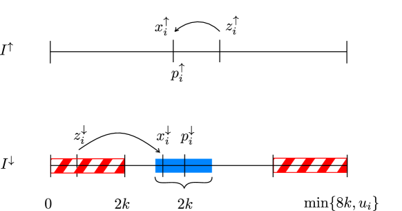
Figure 1: Schematic idea behind the proof of Lemma 5.3 in the case $u_{i}>8k$. We select $p^{\downarrow}_{i}$ such that it is never in the red hatched regions. The property of $p^{\uparrow},p^{\downarrow}$ is that any solution that differs by at most $k$ elements can take the same elements from $I^{\uparrow}$ as $p^{\uparrow}_{i}$. In that case the situation where the optimal solution is of the form $z$ (in the figure) can always be avoided to instead get the situation with $x$.

Proof 5.4.

The proof consists of straightforward, but tedious, calculations; see Figure 1 for an intuition.

By Lemma 2.1 we know that there is a feasible solution $x$ with $\lVert x-p\rVert_{1}\leqslant\mathcal{O}(s)$. Let us use this solution and construct $x^{\uparrow}$ and $x^{\downarrow}$. We consider each index $i\in[n]$ individually and show that there is a split of $x_{i}$ into $x^{\uparrow}_{i}$, $x^{\downarrow}_{i}$ which are feasible for $I^{\uparrow}$, $I^{\downarrow}$, that is, they satisfy the bounds $[0,u^{\uparrow}_{i}]$ and $[0,u^{\downarrow}_{i}]$, and we have that $|x^{\uparrow}_{i}-p^{\uparrow}_{i}|\leqslant 19|x_{i}-p_{i}|/k$. This implies the lemma. To this end, consider two cases based on $|x_{i}-p_{i}|$.

Case 1: $|x_{i}-p_{i}|<k$

In this case we set $x^{\uparrow}_{i}=p^{\uparrow}_{i}$ and $x^{\downarrow}_{i}=x_{i}-kx^{\uparrow}_{i}$. This choice does not contribute anything to the norm $\lVert x^{\uparrow}-p^{\uparrow}\rVert_{1}$ because $x_{i}^{\uparrow}=p_{i}^{\uparrow}$. We need to show that $x^{\uparrow}_{i}$ and $x^{\downarrow}_{i}$ are feasible solutions to the subset sum instances $I^{\uparrow}$ and $I^{\downarrow}$.

Clearly, $x^{\uparrow}_{i}$ is between $0$ and $u^{\uparrow}_{i}=\max\{\lfloor u_{i}/k\rfloor-8,0\}$ in the first two cases of Definition 5.2. In the last case, we have that $4k<p_{i}<u_{i}-4k$ and therefore $0\leqslant\lfloor p_{i}/k\rfloor-2=p^{\uparrow}_{i}$. Furthermore, $p^{\uparrow}_{i}=\lfloor p_{i}/k\rfloor-2<p_{i}/k-3<u_{i}/k-7<\lfloor u_{i}/k\rfloor-8=u^{\uparrow}_{i}$.

Therefore, it remains to show that $x^{\downarrow}_{i}$ is feasible for $I^{\downarrow}$. More precisely, we will prove that:

$$0\leqslant x_{i}-kp^{\uparrow}_{i}\leqslant u_{i}-k\cdot\max\{\left\lfloor u_{i}/k\right\rfloor-8,0\}.$$

To achieve that, we will crucially rely on our choice for $p^{\uparrow}$ in Definition 5.2.

Case 1a: $u_{i}\leqslant 8k$ or $p_{i}\leqslant 8k$

When $u_{i}\leqslant 8k$ or $p_{i}\leqslant 8k$ then the claim follows because $p_{i}^{\uparrow}=x_{i}^{\uparrow}=0$.

Case 1b: $p_{i}\geqslant u_{i}-4k$ and $u_{i}>8k$

In this case we have $p^{\uparrow}_{i}:=\left\lfloor u_{i}/k\right\rfloor-8$. Inequality $x_{i}-kp^{\uparrow}_{i}\geqslant 0$ follows from $x_{i}>p_{i}-k\geqslant u_{i}-5k\geqslant k\lfloor u_{i}/k\rfloor-8k=kp^{\uparrow}_{i}$. Next, we use the fact $x_{i}\leqslant u_{i}$ to conclude $x_{i}-k\left\lfloor u_{i}/k\right\rfloor+8k\leqslant u_{i}-k\left\lfloor u_{i}/k\right\rfloor+8k$.

Case 1c: $4k<p_{i}<u_{i}-4k$ and $u_{i}>8k$

In this case we have $p^{\uparrow}_{i}:=\left\lfloor p_{i}/k\right\rfloor-2$. The inequality $x_{i}>p_{i}-k\geqslant k\left\lfloor p_{i}/k\right\rfloor-k=kp^{\uparrow}_{i}+k$ shows that $x_{i}-kp^{\uparrow}_{i}\geqslant 0$. Next, we use inequality $p_{i}-k\left\lfloor p_{i}/k\right\rfloor<k$ to show that

$$x_{i}-k\left\lfloor p_{i}/k\right\rfloor\leqslant p_{i}-k\left\lfloor p_{i}/k\right\rfloor+k\leqslant 2k<\underbrace{u_{i}-k\left\lfloor u_{i}/k\right\rfloor}_{\geqslant 0}+8k.$$

Case 2: $|x_{i}-p_{i}|\geqslant k$

We set $x^{\uparrow}_{i}:=\min\{\left\lfloor x_{i}/k\right\rfloor,u^{\uparrow}_{i}\}$ and $x^{\downarrow}_{i}:=x_{i}-kx^{\uparrow}_{i}$. Clearly, $0\leqslant x^{\uparrow}_{i}\leqslant u^{\uparrow}_{i}$. Furthermore, $x^{\downarrow}_{i}\geqslant 0$ and if $x^{\uparrow}_{i}=u^{\uparrow}_{i}$ then $x^{\downarrow}_{i}\leqslant u_{i}-ku^{\uparrow}_{i}=u^{\downarrow}_{i}$; otherwise, $x^{\downarrow}_{i}=x_{i}-k\left\lfloor x_{i}/k\right\rfloor<k<u^{\downarrow}_{i}$.

It remains to bound the difference between $x^{\uparrow}_{i}$ and $p^{\uparrow}_{i}$. Note that because of our choice of $p^{\uparrow}$ we have $|p^{\uparrow}_{i}-\left\lfloor p_{i}/k\right\rfloor|\leqslant 8$. Also, $|u^{\uparrow}_{i}-\left\lfloor u_{i}/k\right\rfloor|\leqslant 8$. Therefore,

$$|x^{\uparrow}_{i}-p^{\uparrow}_{i}|\leqslant\big{|}\min\{\left\lfloor x_{i}/k\right\rfloor,u^{\uparrow}_{i}\}-\left\lfloor p_{i}/k\right\rfloor\big{|}+8\leqslant\big{|}\underbrace{\min\{\left\lfloor x_{i}/k\right\rfloor,\left\lfloor u_{i}/k\right\rfloor\}}_{=\left\lfloor x_{i}/k\right\rfloor}-\left\lfloor p_{i}/k\right\rfloor\big{|}+16\\ \leqslant|x_{i}-p_{i}|/k+18.$$

Recall that we assumed $|x_{i}-p_{i}|\geqslant k$. Thus,

$$|x^{\uparrow}_{i}-p^{\uparrow}_{i}|\leqslant 19|x_{i}-p_{i}|/k.$$

Now we are ready to proceed with the algorithmic part and prove Lemma 5.1.

Proof 5.5 (Proof of Lemma 5.1).

Let $t_{p}$ be the value of $p^{\uparrow}$ in $I^{\uparrow}$, that is, $t_{p}:=\sum_{i\in[n]}p^{\uparrow}_{i}s_{i}$. Let $A^{-}$ be the multiset of numbers selected in $p^{\uparrow}$. Moreover, let $A^{+}$ denote all other elements in $I^{\uparrow}$. We now compute

$$S^{+}:=\mathcal{S}(A^{+})\cap[c\cdot s^{5/3}]\;\;\text{ and }\;\;S^{-}:=\mathcal{S}(A^{-})\cap[c\cdot s^{5/3}].$$

Here $c$ is a constant that we will specify later. These sets can be computed in time $\widetilde{\mathcal{O}}(s^{5/3})$ with Bringmann’s algorithm [9]. Next, using FFT we compute the sumset

$$\mathcal{C}(I^{\uparrow}):=\{t_{p}+a-b\mid a\in S^{+},b\in S^{-}\}.$$

Any element in $\mathcal{C}(I^{\uparrow})$ is an integer of the form $t_{p}+a-b$, integer $a$ is the sum of elements not in $p^{\uparrow}$, and integer $t_{p}-b$ is the contribution of elements in $p^{\uparrow}$. This operation takes time $\widetilde{\mathcal{O}}(s^{5/3})$ because the range of values of $S^{+}$ and $S^{-}$ is bounded by $\mathcal{O}(s^{5/3})$. We return set $\mathcal{C}(I^{\uparrow})$ as the set of possible values of the candidates. To recover a solution we will use the fact that Bringmann’s algorithm can recover solutions and the property that we can find a witness to FFT computation in linear time. Since $S^{+}$ and $S^{-}$ are subsets of $[c\cdot s^{5/3}]$ we know that $\mathcal{C}(I^{\uparrow})$ is a subset of $\{t_{p}-c\cdot s^{5/3},\dotsc,t_{p}+c\cdot s^{5/3}\}$. In particular, $|\mathcal{C}(I^{\uparrow})|\leqslant\widetilde{\mathcal{O}}(s^{5/3})$.

It remains to to show that $\mathcal{C}(I^{\uparrow})$ contains some $t^{\prime}$ such that $t-kt^{\prime}\in\mathcal{S}(I^{\downarrow})$ if $t\in\mathcal{S}(I)$. By Lemma 5.3 it suffices to show that $\mathcal{C}(I^{\uparrow})$ contains all values $\sum_{i\in[n]}x_{i}^{\uparrow}s_{i}$ for $x^{\uparrow}$ with $\lVert x^{\uparrow}-p^{\uparrow}\rVert_{1}\leqslant c\cdot s/k$, where $c$ is the constant in the lemma. This holds because $S^{+}$ contains $\sum_{i\in[n]:x^{\uparrow}_{i}\geqslant p^{\uparrow}_{i}}(x_{i}^{\uparrow}-p^{\uparrow}_{i})s_{i}$ and $S^{-}$ contains $\sum_{i\in[n]:x^{\uparrow}_{i}\leqslant p^{\uparrow}_{i}}(p^{\uparrow}_{i}-x_{i}^{\uparrow})s_{i}$.

5.2 Introduction to additive combinatorics methods

In this section we review the structural ideas behind the proof of Theorem 2.5. Next, in Section 5.3 we show how to use them to recover a solution to Subset Sum with multiplicities.

The additive combinatorics structure that we explore is present in the regime when $N^{2}\gg us$. We formalize this assumption as follows:

Definition 5.6 (Density).

We say that a multiset $X$ is $\delta$-dense if it satisfies $|X|^{2}\geqslant\delta us$.

Note that if all numbers in $X$ are divisible by the same integer $d$, then the solutions to Subset Sum are divisible by $d$. Intuitively, this situation is undesirable, because our goal is to exploit the density of the instance. With the next definition we quantify how close we are to the case where almost all numbers in $X$ are divisible by the same number.

Definition 5.7 (Almost Divisor).

We write $X(d):=X\cap d\mathbb{Z}$ to denote the multiset of all numbers in $X$ that are divisible by $d$ and $\overline{X(d)}:=X\setminus X(d)$ to denote the multiset of all numbers in $X$ not divisible by $d$. We say that an integer $d>1$ is an $\alpha$-almost divisor of $X$ if $|\overline{X(d)}|\leqslant\alpha u\Sigma(X)/|X|^{2}$.

Bringmann and Wellnitz [11] show that this situation is not the hardest case.

Lemma 5.8 (Algorithmic Part of [11]).

Given an $\widetilde{\Theta}(1)$-dense multiset $X$ of size $N$ in time $\widetilde{\mathcal{O}}(N)$ we can compute an integer $d\geqslant 1$, such that $X^{\prime}:=X(d)/d$ is $\widetilde{\Theta}(1)$-dense and has no $\widetilde{\Theta}(1)$-almost divisors.

They achieve that with novel prime factorization techniques. This lemma allows them essentially to reduce to the case that there are no $\widetilde{\Theta}(1)$-almost divisors. We will give more details on this in the end of Section 2.3. In our proofs we use the Lemma 5.8 as a blackbox. Next, we focus on the structural part of their arguments.

Structural part

The structural part of [11] states the surprising property. If we are given a sufficiently dense instance with no almost divisors then every set with target within the given region is attainable.

Theorem 5.9 (Structural Part of [11]).

If $X$ is $\widetilde{\Theta}(1)$-dense and has no $\widetilde{\Theta}(1)$-almost divisor then $[\lambda_{X},\ldots,\Sigma(X)-\lambda_{X}]\subseteq\mathcal{S}(X)$ for some $\lambda_{X}=\widetilde{\Theta}(us\Sigma(X)/|X|^{2}))$.

Therefore, Bringmann and Wellnitz [11] after the reduction to the almost-divisor-free setting can simply output YES on every target in the selected region. Our goal is to recover the solution to subset sum and therefore, we need to get into the details of this proof and show that we can efficiently construct it. The crucial insight into this theorem is the following decomposition of a dense multiset.

Lemma 5.10 (Decomposition, see [11, Theorem 4.35]).

Let $X$ be a $\widetilde{\Theta}(1)$-dense multiset of size $n$ that has no $\widetilde{\Theta}(1)$-almost divisor. Then there exists a partition $X=R\uplus A\uplus G$ and an integer $\kappa=\widetilde{\mathcal{O}}(u\Sigma(X)/|X|^{2})$ such that:

• set $\mathcal{S}(R)$ is $\kappa$-complete, i.e., $\mathcal{S}(R)\bmod\kappa=\mathbb{Z}_{\kappa}$,

• set $\mathcal{S}(A)$ contains an arithmetic progression $\mathcal{P}$ of length $2s$ and step size $\kappa$ satisfying $\max\{\mathcal{P}\}\leqslant\widetilde{\mathcal{O}}(us\Sigma(X)/|X|^{2})$,

• the multiset $G$ has sum $\Sigma(G)\geqslant\Sigma(X)/2$.

Now, we sketch the proof of Theorem 5.9 with the decomposition from Lemma 5.10. This is based on the proof in [11].

Proof 5.11 (Sketch of the proof of Theorem 5.9 assuming Lemma 5.10).

We show that any target $t\in[\lambda_{X},\ldots,\Sigma(X)-\lambda_{X}]$ is a subset sum of $X$. For that we will assume without loss of generality that $t\leqslant\Sigma(X)/2$ (note that $t$ is a subset sum if and only if $\Sigma(X)-t$ is). By Lemma 5.10 we get a partition of $X$ into $R\uplus A\uplus G$. We know that $\mathcal{S}(A)$ contains an arithmetic progression $\mathcal{P}\subseteq\mathcal{S}(A)$, with $\mathcal{P}=\{a+\kappa,a+2\kappa,\ldots,a+2s\kappa\}$. We construct a subset of $X$ that sums to $t$ as follows. First, we greedily pick $G^{\prime}\subseteq G$ by iteratively adding elements until:

$$t-\Sigma(G^{\prime})\in[a+\kappa(s+1),a+\kappa(s+1)+s].$$

This is possible because the largest element is bounded by $s$, $t$ is at most $\Sigma(X)/2\leqslant\Sigma(G)$, and $\lambda_{X}$ is selected such that:

$$t\geqslant\lambda_{X}\geqslant a+\kappa(s+1).$$

The next step is to select a subset $R^{\prime}\subseteq R$ that sums up to a number congruent to $(t-\Sigma(G^{\prime})-a)$ modulo $\kappa$. Recall, that set $R$ is $\kappa$-complete, hence such a set must exist. Moreover, w.l.o.g. $R^{\prime}<\kappa$, and $\Sigma(R^{\prime})<\kappa s$. Therefore, we need extra elements of total sum

$$t-\Sigma(G^{\prime}\cup R^{\prime})\in[a+\kappa,a+2\kappa s],\quad\text{and}\quad t-\Sigma(G^{\prime}\cup R^{\prime})\equiv a\mod\kappa.$$

Finally, we note that this is exactly the range of elements of the arithmetic progression $\mathcal{P}$. It means that we can pick a subset $A^{\prime}\subseteq A$, that gives the appropriate element of the arithmetic progression $\mathcal{P}$ and $t=\Sigma(G^{\prime}\cup R^{\prime}\cup A^{\prime})$.

5.3 Recovering a solution

In this section, we show how to recover a solution to Subset Sum. We need to overcome several technical difficulties. First, we need to reanalyze Lemma 5.10 and show that the partition $X=A\uplus R\uplus G$ can be constructed efficiently. This step follows directly from [11]. However, we do not know of an efficient way to construct $\kappa$ and $a$. We show that we do not really need it. Intuitively, for our application we can afford to spend a time $\widetilde{\mathcal{O}}(N+\lambda_{I})$. This observation enables us to use the $\widetilde{\mathcal{O}}(N+t)$ time algorithm of Bringmann [9] to reconstruct the solution. We commence with the observation that the decomposition into $R\uplus A\uplus G$ can be constructed within the desired time.

Claim 2 (Recovering decomposition).

Let $X$ be a $\widetilde{\Theta}(1)$-dense multiset that has no $\widetilde{\Theta}(1)$-almost divisor. Let $K=42480\cdot u\cdot\Sigma(X)\log(2u)/|X|^{2}$. Then in $\widetilde{\mathcal{O}}(N+u\Sigma(X)/|X|^{2})$ time we can explicitly find a partition $X=R\uplus A\uplus G$ such that:

• set $\mathcal{S}(R)$ is $d$-complete for any $d\leqslant K$,

• there exists an integer $\kappa\leqslant K$ such that the set $\mathcal{S}(A)$ contains an arithmetic progression $\mathcal{P}$ of length $2s$ and step size $\kappa$ satisfying $\max\{\mathcal{P}\}\leqslant\widetilde{\mathcal{O}}(us\Sigma(X)/|X|^{2})$,

• the multiset $G$ has sum $\Sigma(G)\geqslant\Sigma(X)/2$.

Proof 5.12 (Proof of Claim 2 based on arguments from [11]).

We follow the proof of Theorem 4.35 in [11]. We focus on the construction of partition $X$ and present only how the construction follows from [11].

To construct the set $R$, Bringmann and Wellnitz use [11, Theorem 4.20]. We start by picking an arbitrary subset $R^{\prime}\subseteq X$ of size $\tau=\widetilde{\Theta}(u\Sigma(X)/|X|^{2})$. Next we generate the set $S$ of all prime numbers $p$ with $p\leqslant\tau$. We can do this in $\widetilde{\mathcal{O}}(\tau)$ time by the sieve of Eratosthenes algorithm [30]. Then, we compute the prime factorization of every number in $R^{\prime}$ by [11, Theorem 3.8] in $\widetilde{\mathcal{O}}(\tau)$ time. This enables us to construct the set $P$ of primes $p$ with $p\leqslant\tau$ such that every $p\in P$ does not divide at least $\tau/2$ numbers in $R^{\prime}$. Bringmann and Wellnitz [11] show that $|P|\leqslant 2\log{s}$. Next, for every $p\in P$ we select an arbitrary subset $R_{p}\subseteq\overline{X(p)}$ of size $|R_{p}|=\tau$. This can be done in $\widetilde{\mathcal{O}}(N)$ time because $|P|=\widetilde{\mathcal{O}}(1)$. Finally Bringmann and Wellnitz [11] construct $R=R^{\prime}\cup\left(\bigcup_{p\in P}R_{p}\right)$. See Theorem 4.20 in [11] for a proof that the constructed $R$ is $d$-complete for any $d\leqslant K$.

To construct set $A$ we do exactly the same as Bringmann and Wellnitz [11] and we pick at most $\left\lfloor n/4\right\rfloor$ smallest elements from $X\setminus R$. At the end we set $G=X\setminus(R\cup A)$. See [11] for a proof that $A$ and $G$ have a desired properties.

Now, we are ready to prove our result about recovering the solution

Lemma 5.13 (Restatement of Lemma 2.6).

Given a multiset $I$ of $N$ elements, in $\widetilde{\mathcal{O}}(N+s^{3/2}u^{1/2})$ time we can construct a data structure that for any $t\in{\rm Nature}$ can decide if $t\in\mathcal{S}(I)$ in time $\mathcal{O}(1)$. Moreover if $t\in\mathcal{S}(I)$ in $\widetilde{\mathcal{O}}(N+s^{3/2}u^{1/2})$ time we can find $X\subseteq I$ with $\Sigma(X)=t$.

In the rest of this section we prove Lemma 2.6. We assume that all considered $t$ are at most $\Sigma(I)/2$ because for larger $t$ we can ask about $\Sigma(I)-t$ instead. Let $\lambda_{I}$ and be defined as in Theorem 2.5. When the total sum of the elements $\Sigma(I)$ is bounded by $\widetilde{\mathcal{O}}(s^{3/2}u^{1/2})$, Bringmann’s algorithm [9] computes $\mathcal{S}(I)$ and retrieves the solution in the declared time. Therefore, we can assume that $s^{3/2}u^{1/2}\leqslant\widetilde{\mathcal{O}}(|I|s)$. In particular, this means that $\sqrt{us}\leqslant\widetilde{\mathcal{O}}(|I|)$ and the set $I$ is $\widetilde{\Theta}(1)$-dense. Hence,

$$\lambda_{I}\leqslant\widetilde{\mathcal{O}}\left(\frac{us\Sigma(I)}{|I|^{2}}\right)\leqslant\widetilde{\mathcal{O}}\left(\frac{us^{2}}{|I|}\right)\leqslant\widetilde{\mathcal{O}}(u^{1/2}s^{3/2}).$$

This means, that we can afford $\widetilde{\mathcal{O}}(\lambda_{I})$ time. In time $\widetilde{\mathcal{O}}(|I|+\lambda_{I})$ we can find all subset sums in $\mathcal{S}(I)$ that are smaller than $\widetilde{\Theta}(\lambda_{I})$ using Bringmann’s algorithm. Additionally, when $t\leqslant\widetilde{\Theta}(\lambda_{I})$ Bringmann’s algorithm can find $X\subseteq I$ in the output sensitive time.

We are left with answering queries about targets greater than $\lambda_{I}$. To achieve that within $\widetilde{\mathcal{O}}(\lambda_{I})$-time preprocessing we use the Additive Combinatorics result from [11].

Observe, that if we were interested in a data structure that works in $\widetilde{\mathcal{O}}(N+\lambda_{I})\leqslant\widetilde{\mathcal{O}}(N+s^{3/2}u^{1/2})$ and decides if $t\in\mathcal{S}(I)$ we can directly use [11] as a blackbox. Therefore, from now, we show that we can also reconstruct the solution in $\widetilde{\mathcal{O}}(N+\lambda_{I})$ time.

Claim 3.

We can find a set $X\subseteq I$ with $\Sigma(X)=t$ in $\widetilde{\mathcal{O}}(N+\lambda_{I})$ time for any $t\in[\lambda_{I},\Sigma(I)/2]$ if such an $X$ exists.

Proof 5.14.

First, we use Lemma 5.8 to find an integer $d\geqslant 1$, such that set $I^{\prime}:=I(d)/d$ has no $\widetilde{\Theta}(1)$-almost divisor and is $\widetilde{\Theta}(1)$-dense. Observe, that the integer $d$ can be found in $\widetilde{\mathcal{O}}(N)$ time and set $I^{\prime}$ can be constructed in $\widetilde{\mathcal{O}}(N)$ time.

Bringmann and Wellnitz [11, Theorem 3.5] prove that (recall that $I$ is $\widetilde{\Theta}(1)$-dense and $t\geqslant\lambda_{I}$):

$$t\in\mathcal{S}(I)\text{ if and only if }t\bmod d\in(\mathcal{S}(I)\bmod d).$$

Therefore, the first step of our algorithm is to use Axiotis et al. [4] to decide if $t\bmod d\in(\mathcal{S}(I)\bmod d)$ and recover set $D\subseteq I\setminus I(d)$ if such a set exists (Axiotis et al. [4] enables to recover solution and by density assumption it works in $\widetilde{\mathcal{O}}(N)$ time).

If such a set exists by reasoning in [11] we know that a solution must exist (otherwise we output NO). We are left with recovering set $K\subseteq I^{\prime}$ with $\Sigma(K):=(t-\Sigma(D))/d$.

Next, we use Claim 2 to find a partition $I^{\prime}=R\uplus A\uplus G$. We can achieve that in $\widetilde{\mathcal{O}}(u\Sigma(I^{\prime})/|I^{\prime}|^{2})\ll\widetilde{\mathcal{O}}(N+\lambda_{I})$ time. Ideally, we would like to repeat the reasoning presented in the proof of Theorem 5.9. Unfortunately, we do not know how to explicitly construct $a$ and $\kappa$ within the given time. Nevertheless, Theorem 5.9 guarantees that $t\in\mathcal{S}(I)$ and that such integers $a$ and $\kappa$ exist.

Based on the properties of sets in Theorem 5.9 we have

$$t\in\mathcal{S}(G\uplus R\uplus A)=\mathcal{S}(G)\oplus(\mathcal{S}(R\cup A)\cap[0,\widetilde{\mathcal{O}}(\lambda_{I})]).$$

With a Bringmann’s algorithm we can compute the set $T:=\mathcal{S}(R\cup A)\cap[0,\widetilde{\mathcal{O}}(\lambda_{I})]$ in $\widetilde{\mathcal{O}}(N+\lambda_{I})$ time. Now, recall that in the proof of Theorem 5.9 we have chosen set $G^{\prime}\subseteq G$ greedily to satisfy $\Sigma(G^{\prime})\geqslant t-a-\kappa(s+1)$ for some $a,\kappa$ and $s$. Therefore it is enough to iterate over every greedily chosen $G^{\prime}\subseteq G$ and check whether $t-\Sigma(G^{\prime})\in T$. Notice that there are only $N$ options for $G^{\prime}$ that can be generated in $\mathcal{O}(N+\lambda_{I})$ time. For each of them we can check whether $t-\Sigma(G^{\prime})\in T$ in $\mathcal{O}(1)$ time because we have access to $T$. If we find such a set, we just report $K:=G^{\prime}\cup T^{\prime}$, where $T^{\prime}\subseteq R\cup A$ with $\Sigma(T^{\prime})+\Sigma(G^{\prime})=t$.

This concludes the proof of Lemma 2.6.

References

- [1] Amir Abboud, Karl Bringmann, Danny Hermelin, and Dvir Shabtay. SETH-based lower bounds for subset sum and bicriteria path. In Proceedings of the Thirtieth Annual ACM-SIAM Symposium on Discrete Algorithms, SODA 2019, pages 41–57. SIAM, 2019. doi:10.1137/1.9781611975482.3.
- [2] Alok Aggarwal, Maria M. Klawe, Shlomo Moran, Peter W. Shor, and Robert E. Wilber. Geometric applications of a matrix-searching algorithm. Algorithmica, 2:195–208, 1987. doi:10.1007/BF01840359.
- [3] Kyriakos Axiotis, Arturs Backurs, Karl Bringmann, Ce Jin, Vasileios Nakos, Christos Tzamos, and Hongxun Wu. Fast and simple modular subset sum. In 4th Symposium on Simplicity in Algorithms, SOSA 2021, pages 57–67. SIAM, 2021. doi:10.1137/1.9781611976496.6.
- [4] Kyriakos Axiotis, Arturs Backurs, Ce Jin, Christos Tzamos, and Hongxun Wu. Fast modular subset sum using linear sketching. In Proceedings of the Thirtieth Annual ACM-SIAM Symposium on Discrete Algorithms, SODA 2019, pages 58–69, 2019. doi:10.1137/1.9781611975482.4.
- [5] Kyriakos Axiotis and Christos Tzamos. Capacitated dynamic programming: Faster knapsack and graph algorithms. In 46th International Colloquium on Automata, Languages, and Programming, ICALP 2019, volume 132 of LIPIcs, pages 19:1–19:13, 2019. doi:10.4230/LIPIcs.ICALP.2019.19.
- [6] MohammadHossein Bateni, MohammadTaghi Hajiaghayi, Saeed Seddighin, and Cliff Stein. Fast algorithms for knapsack via convolution and prediction. In Proceedings of the 50th Annual ACM SIGACT Symposium on Theory of Computing, STOC 2018, pages 1269–1282, 2018. doi:10.1145/3188745.3188876.
- [7] Richard Bellman. Dynamic Programming. Princeton University Press, Princeton, NJ, USA, 1957.
- [8] Manuel Blum, Robert W. Floyd, Vaughan R. Pratt, Ronald L. Rivest, and Robert Endre Tarjan. Time bounds for selection. J. Comput. Syst. Sci., 7(4):448–461, 1973. doi:10.1016/S0022-0000(73)80033-9.
- [9] Karl Bringmann. A near-linear pseudopolynomial time algorithm for subset sum. In Proceedings of the Twenty-Eighth Annual ACM-SIAM Symposium on Discrete Algorithms, SODA 2017, pages 1073–1084. SIAM, 2017. doi:10.1137/1.9781611974782.69.
- [10] Karl Bringmann and Vasileios Nakos. Top-k-convolution and the quest for near-linear output-sensitive subset sum. In Proccedings of the 52nd Annual ACM SIGACT Symposium on Theory of Computing, STOC 2020, pages 982–995. ACM, 2020. doi:10.1145/3357713.3384308.
- [11] Karl Bringmann and Philip Wellnitz. On near-linear-time algorithms for dense subset sum. In Proceedings of the 2021 ACM-SIAM Symposium on Discrete Algorithms, SODA 2021, pages 1777–1796. SIAM, 2021. doi:10.1137/1.9781611976465.107.
- [12] Jean Cardinal and John Iacono. Modular subset sum, dynamic strings, and zero-sum sets. In 4th Symposium on Simplicity in Algorithms, SOSA 2021, pages 45–56. SIAM, 2021. doi:10.1137/1.9781611976496.5.
- [13] Timothy M. Chan and Qizheng He. More on change-making and related problems. In 28th Annual European Symposium on Algorithms, ESA 2020, pages 29:1–29:14, 2020. doi:10.4230/LIPIcs.ESA.2020.29.
- [14] Marek Cygan, Holger Dell, Daniel Lokshtanov, Dániel Marx, Jesper Nederlof, Yoshio Okamoto, Ramamohan Paturi, Saket Saurabh, and Magnus Wahlström. On problems as hard as CNF-SAT. ACM Trans. Algorithms, 12(3):41:1–41:24, 2016. URL: https://doi.org/10.1145/2925416.
- [15] Marek Cygan, Marcin Mucha, Karol Węgrzycki, and Michał Włodarczyk. On problems equivalent to -convolution. ACM Trans. Algorithms, 15(1):14:1–14:25, 2019. doi:10.1145/3293465.
- [16] Friedrich Eisenbrand and Robert Weismantel. Proximity results and faster algorithms for integer programming using the Steinitz lemma. ACM Trans. Algorithms, 16(1):5:1–5:14, 2020. doi:10.1145/3340322.
- [17] Zvi Galil and Oded Margalit. An almost linear-time algorithm for the dense subset-sum problem. SIAM J. Comput., 20(6):1157–1189, 1991. doi:10.1137/0220072.
- [18] Michel X. Goemans and Thomas Rothvoss. Polynomiality for bin packing with a constant number of item types. J. ACM, 67(6):38:1–38:21, 2020. doi:10.1145/3421750.
- [19] Klaus Jansen and Lars Rohwedder. On integer programming and convolution. In 10th Innovations in Theoretical Computer Science Conference, ITCS 2019, pages 43:1–43:17, 2019. doi:10.4230/LIPIcs.ITCS.2019.43.
- [20] Ce Jin, Nikhil Vyas, and Ryan Williams. Fast low-space algorithms for subset sum. In Proceedings of the 2021 ACM-SIAM Symposium on Discrete Algorithms, SODA 2021, pages 1757–1776. SIAM, 2021. doi:10.1137/1.9781611976465.106.
- [21] Ce Jin and Hongxun Wu. A simple near-linear pseudopolynomial time randomized algorithm for subset sum. In 2nd Symposium on Simplicity in Algorithms, SOSA@SODA 2019, pages 17:1–17:6, 2019. doi:10.4230/OASIcs.SOSA.2019.17.
- [22] Hans Kellerer and Ulrich Pferschy. Improved dynamic programming in connection with an FPTAS for the knapsack problem. J. Comb. Optim., 8(1):5–11, 2004. doi:10.1023/B:JOCO.0000021934.29833.6b.
- [23] Hans Kellerer, Ulrich Pferschy, and David Pisinger. Knapsack problems. Springer, 2004. doi:10.1007/978-3-540-24777-7.
- [24] Konstantinos Koiliaris and Chao Xu. Faster pseudopolynomial time algorithms for subset sum. ACM Trans. Algorithms, 15(3):40:1–40:20, 2019. doi:10.1145/3329863.
- [25] Marvin Künnemann, Ramamohan Paturi, and Stefan Schneider. On the fine-grained complexity of one-dimensional dynamic programming. In 44th International Colloquium on Automata, Languages, and Programming, ICALP 2017, pages 21:1–21:15, 2017. doi:10.4230/LIPIcs.ICALP.2017.21.
- [26] Eugene L. Lawler. Fast approximation algorithms for knapsack problems. Math. Oper. Res., 4(4):339–356, 1979. doi:10.1287/moor.4.4.339.
- [27] Daniel Lokshtanov and Jesper Nederlof. Saving space by algebraization. In Proceedings of the 42nd ACM Symposium on Theory of Computing, STOC 2010, pages 321–330. ACM, 2010. doi:10.1145/1806689.1806735.
- [28] David Pisinger. Linear time algorithms for knapsack problems with bounded weights. J. Algorithms, 33(1):1–14, 1999. doi:10.1006/jagm.1999.1034.
- [29] Krzysztof Potępa. Faster deterministic modular subset sum, 2020. arXiv:2012.06062.
- [30] Jonathan Sorenson. An introduction to prime number sieves. Technical report, University of Wisconsin-Madison Department of Computer Sciences, 1990.
- [31] Arie Tamir. New pseudopolynomial complexity bounds for the bounded and other integer knapsack related problems. Oper. Res. Lett., 37(5):303–306, 2009. doi:10.1016/j.orl.2009.05.003.