Key Assistance, Key Agreement, and Layered Secrecy for Bosonic Broadcast Channels

Abstract

Secret-sharing building blocks based on quantum broadcast communication are studied. The confidential capacity region of the pure-loss bosonic broadcast channel is determined, both with and without key assistance, and an achievable region is established for the lossy bosonic broadcast channel. If the main receiver has a transmissivity of $\eta<\frac{1}{2}$, then confidentiality solely relies on the key-assisted encryption of the one-time pad. We also address conference key agreement for the distillation of two keys, a public key and a secret key. A regularized formula is derived for the key-agreement capacity region in finite dimensions. In the bosonic case, the key-agreement region is included within the capacity region of the corresponding broadcast channel with confidential messages. We then consider a network with layered secrecy, where three users with different security ranks communicate over the same broadcast network. We derive an achievable layered-secrecy region for a pure-loss bosonic channel that is formed by the concatenation of two beam splitters.

I Introduction

Physical-layer security requires the communication of private information to be secret regardless of the computational capabilities of a potential eavesdropper [1, 2]. Secret-key agreement is a promising method to achieve this goal, whereby the sender and the receiver generate a secret key before communication takes place. Maurer [3] and Ahlswede and Csiszár [4] have independently developed and analyzed the information-theoretic model for such a protocol, whereby Alice and Bob use pre-existing correlations, along with a public insecure channel, to generate a secret key. Devetak and Winter [5] considered the quantum counterpart of key distillation from a shared quantum state and public classical communication. Conference key agreement protocols [6], also known as multi-party key distribution are particularly relevant to this work. In this framework, the aim is to distribute a common key between several users, allowing them to broadcast secure messages in a network (see also [7, 8]). In practice, quantum key distribution (QKD) is among the most mature quantum technologies with an information-theoretic basis [9], as it is already implemented in experiments [10, 11, 12, 13], and in commercial use as well [14, 15]. Most QKD implementations are based on optical communication, either with optical fibers or in free space [16, 17]. A QKD protocol aims to distribute a secret symmetric key between authorized partners, with no assumption regarding the communication channel but the laws of quantum mechanics [18, 19]. The key can later be used to communicate using classical encryption schemes, such as the one-time pad (OTP) cypher. As shown by Shannon [20], information-theoretic security can be guaranteed if and only if the entropy of the key string is at least as large as the message length. Usually, the cryptographic analysis is not restricted to a given noise model. Here, on the other hand, we will incorporate the OTP cypher within our network coding scheme for communication over a noisy channel. Classical channel coding with key assistance, i.e., given a pre-shared key, is studied, e.g., in [21, 22, 23].

In some noise models, assuming that the channel statistics are known, communication can also be secured without key assistance. The broadcast channel with confidential messages is a network setting that involves transmission of information to two users, such that part of the information should be accessible for both users, while the other part is only intended for one of them. In commercial terms, those components can be thought of as basic and premium packages, where the latter may require an additional subscription fee. Confidentiality requires that the non-subscribed receiver cannot decode the private component. In the classical model, the sender transmits a sequence $X^{n}$ over a given memoryless broadcast channel $p_{Y,Z|X}$, such that the output sequences $Y^{n}$ and $Z^{n}$ are decoded by two independent receivers. The transmission encodes two types of messages, a common message sent to both receivers at rate $R_{0}$, and a private message sent to Receiver $Y$ at rate $R_{1}$, while eavesdropped by Receiver $Z$. This model was first introduced by Csiszár and Körner [24], who showed that the confidential capacity region is given by

$$\mathcal{C}(p_{Y,Z|X})=\bigcup_{p_{U,V}p_{X|V}}\left\{\begin{array}[]{rl}(R_{0},R_{1})\,:\;R_{0}\leq&\min\left(I(U;Y)\,,\;I(U;Z)\right)\\ R_{1}\leq&I(V;Y|U)-I(V;Z|U)\end{array}\right\}$$ (3)

where $U$ and $V$ are auxiliary random variables. A recent overview of information-theoretic security and its applications can be found in [25] (see also [26, 27]). The broadcast channel with layered decoding and secrecy is a generalization of the degraded broadcast channel with confidential messages [28, 29, 30]. The model describes a network in which multiple users have different credentials to access confidential information. Zou et al. [30] give two examples for practical applications. The first example is a WiFi network of an agency, in which a user is allowed to receive files up to a certain security clearance but should be kept ignorant of classified files that require a higher security level. As pointed out in [30], the agency can set the channel quality on a clearance basis by assigning more communication resources to users with a higher security clearance. The second example in [30] is a social network in which one user wishes to share more information with close friends and less information with others. Tahmasbi et al. [31] have further demonstrated that, for some adversarial models with feedback, the layered-secrecy structure allows the provision of secrecy in hindsight, deferring the decisions as to which bits are secret to a later stage. Connections between confidential channel codes and other cryptographic protocols, such as advantage distillation, information reconciliation, and privacy amplification, can be found e.g., in [32, 33, 2].

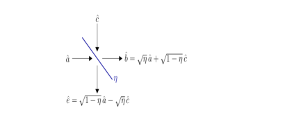
Figure 1: The beam splitter relation of the single-mode bosonic broadcast channel.

Optical communication forms the backbone of the Internet [34, 35, 36, 37]. The bosonic channel is a simple quantum-mechanical model for optical communication over free space or optical fibers [38, 39]. An optical communication system consists of a modulated source of photons, the optical channel, and an optical detector. For a single-mode bosonic broadcast channel, the channel input is an electromagnetic field mode with annihilation operator $\hat{a}$, and the output is a pair of modes with annihilation operators $\hat{b}$ and $\hat{e}$. The annihilation operators correspond to the transmitter (Alice), the legitimate receiver of the common and confidential information (Bob), and the receiver that eavedrops on the confidential information (Eve), respectively. The input-output relation of the bosonic broadcast channel in the Heisenberg picture [40] is given by

$$\hat{b} =\sqrt{\eta}\,\hat{a}+\sqrt{1-\eta}\,\hat{c}$$ (4)

$$\hat{e} =\sqrt{1-\eta}\,\hat{a}-\sqrt{\eta}\,\hat{c}$$ (5)

where $\hat{c}$ is associated with the environment noise and the parameter $\eta$ is the transmissivity, $0\leq\eta\leq 1$, which captures, for instance, the length of the optical fiber and its absorption length [41]. The relation above corresponds to the outputs of a beam splitter, as illustrated in Figure 1. The bosonic channel can be viewed as the quantum counterpart of the classical channel with additive white Gaussian noise (AWGN), which is a well-known model in classical communications [42]. Among others, the Gaussian broadcast channel describes the wide-band thermal noise in the receiver electronic circuits for two remote receiving antennas [43]. As the bosonic broadcast channel, from $A$ to $BE$ (jointly), is isometric, it does not model the distortion introduced by the communication medium [44]. Instead, the bosonic broadcast channel models the de-modulation process at the destination location, where the optical signal is converted into two signals for two independent users by a beam splitter. In a lossy bosonic channel, the noise mode $\hat{c}$ is in a Gibbs thermal state, while, in a pure-loss bosonic channel, the noise mode is in the vacuum state. The channel is called ‘lossy’ or ‘pure-loss’ since the marginal channels, from $A$ to $B$, and from $A$ to $E$, are non-reversible and involve loss of photons in favor of the other receiver.

The broadcast channel with confidential messages can be viewed as a generalization of the wiretap channel [24] [45, Section 22.1.3]. Devetak [46] and Cai et al. [47] addressed the quantum wiretap channel without key assistance and established a regularized characterization of the secrecy capacity. Connections to the coherent information of a quantum point to point channel were drawn in [5]. In general, the secrecy capacity is not additive, hence regularization is necessary [48, 49]. A single-letter characterization was established in the special cases of entanglement-breaking channels [50], as well as the less noisy and more capable wiretap channels [51]. Qi et al. [52] determined the entanglement-assisted secrecy capacity of the quantum wiretap channel (see also [53, 54]). Davis et al. [55] considered an energy-constrained setting, and Boche et al. [56, 57] studied the quantum wiretap channel with an active jammer. Hsieh et al. [58] and Wilde [59] presented a regularized formula for the secret-key-assisted quantum wiretap channel. Furthermore, the capacity-equivocation region was established, characterizing the tradeoff between secret key consumption and private classical communication [58, 59] (see also [50][60, Section 23.5.3]). In [46], Devetak considered entanglement generation using a secret-key-assisted quantum channel. The quantum Gel’fand-Pinsker wiretap channel is considered in [61] and other related scenarios can be found in [62, 63, 64]. Secrecy in the form of quantum state masking was recently considered in [65]. Key distillation is further considered in [66, 67, 68]. Quantum broadcast channels were studied in various settings as well, e.g., [69, 70, 71, 72, 73, 74, 75, 76, 77, 78, 79]. Yard et al. [69] derived the superposition inner bound and determined the capacity region for the degraded classical-quantum broadcast channel. Entanglement generation is considered in [69] as well. Wang et al. [71] used the previous characterization to determine the capacity region for Hadamard broadcast channels as well. Dupuis et al. [72] developed the entanglement-assisted version of Marton’s region for users with independent messages. Bosonic broadcast channels are considered in [80, 81, 82, 83, 66, 84, 85]. The quantum broadcast and multiple access channels with confidential messages were recently considered by Salek et al. [86, 87] and Aghaee et al. [88], respectively (see also [89]). Other security settings of transmission over bosonic channels include covert communication [90, 91, 92], optical QKD [68, 93, 94, 95], and entanglement distillation [96, 83].

In this paper, we study secrecy-sharing building blocks that are based on quantum broadcast communication. We begin with the quantum broadcast channel with confidential messages. We consider two scenarios, either with or without shared key assistance. In particular, we determine the confidential capacity region of the pure-loss bosonic broadcast channel in both settings, as depicted in Figure 5, under the assumption of the long-standing minimum output-entropy conjecture, and we establish an achievable region for the lossy bosonic channel. The main technical challenge is in the converse proof, which requires the conjecture. The achievability proof is based on rate-splitting, combining the “superposition coding” strategy with the OTP cypher using the shared key. The converse proof relies on the long-standing minimum output-entropy conjecture, which is known to hold in special cases [77]. Without key assistance, confidential transmission is only possible if Bob’s channel has a higher transmissivity than Eve’s channel, i.e., $\eta>\frac{1}{2}$. Otherwise, if Bob’s channel is noisier than Eve’s, i.e., $\eta<\frac{1}{2}$, then confidentiality solely relies on the key-assisted encryption of the OTP.

Next, we address key agreement for the distillation and distribution of two keys. The public key is distributed between Alice, Bob, and Eve, while the confidential key is only meant for Alice and Bob, and must be hidden from Eve. Such a protocol can be viewed as a conference key agreement [6], or multi-party key distribution. We obtain a regularized formula for the key-agreement capacity region for the distillation of public and secret keys. We then consider quantum layered secrecy, whereby Alice communicates with three receivers, Bob, Eve 1, and Eve 2. The information has different confidentiality layers, which are labeled by ‘0’, ‘1’, and ’2’. In Layer 0, we have a common message that is intended for all three receivers. In the next layer, the confidential message is decoded by Bob and Eve 1 but should remain hidden from Eve 2. Finally, the top-secret message of Layer 2 is only decoded by Bob, while remaining confidential from both Eve 1 and Eve 2. We derive a regularized formula for the layered-secrecy capacity region of the degraded quantum broadcast channel in finite dimensions and an achievable region for the pure-loss bosonic broadcast channel.

II Definitions and Related Work

II-A Notation, States, and Information Measures

We use the following notation conventions. Script letters $\mathcal{X},\mathcal{Y},\mathcal{Z},...$ are used for finite sets. Lowercase letters $x,y,z,\ldots$ represent constants and values of classical random variables, and uppercase letters $X,Y,Z,\ldots$ represent classical random variables. The distribution of a random variable $X$ is specified by a probability mass function (pmf) $p_{X}(x)$ over a finite set $\mathcal{X}$. We use $x^{j}=(x_{1},x_{2},\ldots,x_{j})$ to denote a sequence of letters from $\mathcal{X}$. A random sequence $X^{n}$ and its distribution $p_{X^{n}}(x^{n})$ are defined accordingly. The type $\hat{P}_{x^{n}}$ of a given sequence $x^{n}$ is defined as the empirical distribution $\hat{P}_{x^{n}}(a)=N(a|x^{n})/n$ for $a\in\mathcal{X}$, where $N(a|x^{n})$ is the number of occurrences of the symbol $a$ in the sequence $x^{n}$. A type class is denoted by $\tau_{n}(\hat{P})=\{x^{n}\,:\;\hat{P}_{x^{n}}=\hat{P}\}$. For a pair of integers $i$ and $j$, $1\leq i\leq j$, we write a discrete interval as $[i:j]=\{i,i+1,\ldots,j\}$. In the continuous case, we use the cumulative distribution function $F_{Z}(z)=\Pr\left(Z\leq z\right)$ for $z\in\mathbb{R}$, or alternatively, the probability density function (pdf) $f_{Z}(z)$, when it exists. We write $Z\sim\mathcal{N}_{\mathbb{R}}(\mu,\sigma^{2})$ to indicate that $Z$ is a real-valued Gaussian variable, with $f_{Z}(z)=\frac{1}{\sqrt{2\pi\sigma^{2}}}e^{-(z-\mu)^{2}/2\sigma^{2}}$. A complex-valued Gaussian variable $\alpha\sim\mathcal{N}_{\mathbb{C}}(0,\sigma^{2})$ can be expressed as $\alpha=X+\textrm{i}Y$ where $X,Y\sim\mathcal{N}_{\mathbb{R}}(0,\sigma^{2})$ are statistically independent.

The state of a quantum system $A$ is a density operator $\rho$ on the Hilbert space $\mathcal{H}_{A}$. A density operator is an Hermitian, positive semidefinite operator, with unit trace, i.e., $\rho^{\dagger}=\rho$, $\rho\succeq 0$, and $\mathrm{Tr}(\rho)=1$. The trace distance between two density operators $\rho$ and $\sigma$ is $\left\lVert\rho-\sigma\right\rVert_{1}$ where $\left\lVert F\right\rVert_{1}=\mathrm{Tr}(\sqrt{F^{\dagger}F})$. Define the quantum entropy of the density operator $\rho$ as $H(\rho)\triangleq-\mathrm{Tr}[\rho\log(\rho)]$. Consider the state of a pair of systems $A$ and $B$ on the tensor product $\mathcal{H}_{A}\otimes\mathcal{H}_{B}$ of the corresponding Hilbert spaces. Given a bipartite state $\sigma_{AB}$, define the quantum mutual information as

$$I(A;B)_{\sigma}=H(\sigma_{A})+H(\sigma_{B})-H(\sigma_{AB})\,.$$ (6)

Furthermore, conditional quantum entropy and mutual information are defined by $H(A|B)_{\sigma}=H(\sigma_{AB})-H(\sigma_{B})$ and $I(A;B|C)_{\sigma}=H(A|C)_{\sigma}+H(B|C)_{\sigma}-H(A,B|C)_{\sigma}$, respectively.

A detailed description of (continuous-variable) bosonic systems can be found in [38]. Here, we only define the notation for the quantities that we use. We use hat-notation, e.g., $\hat{a}$, $\hat{b}$, $\hat{e}$, to denote operators that act on a quantum state. The single-mode Hilbert space is spanned by the Fock basis $\{|n\rangle\}_{n=0}^{\infty}$. Each $|n\rangle$ is an eigenstate of the number operator $\hat{n}=\hat{a}^{\dagger}\hat{a}$, where $\hat{a}$ is the bosonic field annihilation operator. In particular, $|0\rangle$ is the vacuum state of the field. The creation operator $\hat{a}^{\dagger}$ creates an excitation: $\hat{a}^{\dagger}|n\rangle=\sqrt{n+1}|n+1\rangle$, for $n\geq 0$. Reversely, the annihilation operator $\hat{a}$ takes away an excitation: $\hat{a}|n+1\rangle=\sqrt{n+1}|n\rangle$. A coherent state $|\alpha\rangle$, where $\alpha\in\mathbb{C}$, corresponds to an oscillation of the electromagnetic field, and it is the outcome of applying the displacement operator to the vacuum state, i.e., $|\alpha\rangle=D(\alpha)|0\rangle$, which resembles the creation operation, with $D(\alpha)\equiv\exp(\alpha\hat{a}^{\dagger}-\alpha^{*}\hat{a})$. A thermal state $\tau(N)$ is a Gaussian mixture of coherent states, where

$$\tau(N)\equiv\int_{\mathbb{C}}d^{2}\alpha\frac{e^{-|\alpha|^{2}/N}}{\pi N}|\alpha\rangle\langle\alpha|=\frac{1}{N+1}\sum_{n=0}^{\infty}\left(\frac{N}{N+1}\right)^{n}|n\rangle\langle n|$$ (7)

given an average photon number $N\geq 0$.

II-B Quantum Broadcast Channel

A quantum broadcast channel maps a quantum state at the sender system to a quantum state at the receiver systems. Here, we consider a channel with two receivers. Formally, a quantum broadcast channel is a linear, completely positive, trace-preserving map $\mathcal{L}_{A\rightarrow BE}$ corresponding to a quantum physical evolution. We assume that the channel is memoryless. That is, if the system $A^{n}=(A_{1},\ldots,A_{n})$ are sent through $n$ channel uses, then the input state $\rho_{A^{n}}$ undergoes the tensor product mapping $\mathcal{L}_{A^{n}\rightarrow B^{n}E^{n}}\equiv\mathcal{L}_{A\rightarrow BE}^{\otimes n}$. The marginal channel $\mathcal{L}^{(1)}_{A\rightarrow B}$ is defined by

$$\mathcal{L}_{A\rightarrow B}^{(1)}(\rho_{A})=\mathrm{Tr}_{E}\left(\mathcal{L}_{A\rightarrow BE}(\rho_{A})\right)$$ (8)

for Receiver 1, and similarly $\mathcal{L}_{A\rightarrow E}^{(2)}$ for Receiver 2. One may say that $\mathcal{L}_{A\rightarrow BE}$ is an extension of $\mathcal{L}^{(1)}_{A\rightarrow B}$ and $\mathcal{L}^{(2)}_{A\rightarrow E}$. The transmitter, Receiver 1, and Receiver 2 are often referred to as Alice, Bob, and Eve, respectively.

A quantum broadcast channel is degraded if there exists a degrading channel $\mathcal{D}_{B\rightarrow E}$ such that

$$\mathcal{L}^{(2)}_{A\rightarrow E}\equiv\mathcal{D}_{B\rightarrow E}\circ\mathcal{L}^{(1)}_{A\rightarrow B}\,.$$ (9)

We also say that Eve’s channel $\mathcal{L}^{(2)}_{A\rightarrow E}$ is degraded with respect to Bob’s channel $\mathcal{L}^{(1)}_{A\rightarrow B}$. Intuitively, this means that Eve receives a noisier signal than Bob. In the opposite direction, a broadcast channel is called reversely degraded if $\mathcal{L}^{(1)}_{A\rightarrow B}$ is degraded with respect to $\mathcal{L}^{(2)}_{A\rightarrow E}$.

Consider a quantum channel $\mathcal{N}_{A\rightarrow B}$ with a single receiver. Every quantum channel $\mathcal{N}_{A\rightarrow B}$ has a Stinespring dilation $\mathcal{U}^{\,\mathcal{N}}_{A\rightarrow BK}$, where $K$ is a reference system which is often associated with the receiver’s environment. The broadcast channel $\mathcal{U}^{\,\mathcal{N}}_{A\rightarrow BK}$ is an isometric extension of $\mathcal{N}_{A\rightarrow B}$, i.e.,

$$\mathcal{U}^{\,\mathcal{N}}_{A\rightarrow BK}(\rho_{A})=U\rho_{A}U^{\dagger}$$ (10)

$${\mathcal{N}}_{A\rightarrow B}(\rho_{A})=\mathrm{Tr}_{K}(U\rho_{A}U^{\dagger})$$ (11)

where the operator $U$ is an isometry, i.e., $U^{\dagger}U=\text{1}$. The channel $\widehat{\mathcal{N}}_{A\rightarrow K}(\rho_{A})=\mathrm{Tr}_{B}(U\rho_{A}U^{\dagger})$ is called a complementary channel for ${\mathcal{N}}_{A\rightarrow B}$.

Remark 1.

If the broadcast channel $\mathcal{L}_{A\rightarrow BE}$ is isometric, i.e., $\mathcal{L}_{A\rightarrow BE}(\rho_{A})=U\rho_{A}U^{\dagger}$ for some isometry $U$, then the marginal channels are complementary to each other. In this case Eve’s system $E$ can be thought of as Bob’s environment. In particular, this is the case for the bosonic broadcast channel. The bosonic isometry is specified by [77]

$$U_{\eta}=\exp\left((\hat{a}^{\dagger}\hat{c}-\hat{c}^{\dagger}\hat{a})\arccos\sqrt{\eta}\right)\,.$$ (12)

The bosonic broadcast channel is degraded if $\eta\geq\frac{1}{2}$, and reversely degraded if $\eta\leq\frac{1}{2}$. In the degraded case, $\eta\geq\frac{1}{2}$, the degrading channel is simply a second beam splitter with transmissivity

$$\eta^{\prime}=\frac{1-\eta}{\eta}\,.$$ (13)

This is illustrated in Figure 2. Based on [97] (see derivation in the proof of Lemma 3.2 therein), the state of the output mode $\hat{e}^{\prime}$ is the same as that of $\hat{e}$. Thereby, $\mathcal{L}^{(2)}_{A\rightarrow E}\equiv\mathcal{D}_{B\rightarrow E^{\prime}}\circ\mathcal{L}^{(1)}_{A\rightarrow B}$, where $\mathcal{D}_{B\rightarrow E^{\prime}}$ is the bosonic channel corresponding to the second beam splitter.

Figure 2: The degraded representation of the bosonic broadcast channel. Bob’s output mode is directed into another beam splitter with transmissivity $\eta^{\prime}=\frac{1-\eta}{\eta}$. The state of the output mode $\hat{e}^{\prime}$ is the same as that of $\hat{e}$.

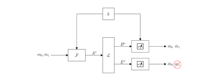
Figure 3: The quantum broadcast channel with confidential messages and key assistance. The sender Alice has the system $A^{n}$, and the receivers Bob and Eve have the systems $B^{n}$ and $E^{n}$, respectively. Alice and Bob share a random key $k$, which is not known to Eve. Alice chooses a common message $m_{0}$ that is intended for both users and a confidential message $m_{1}$ for Bob. She encodes the messages by applying the encoding map $\mathcal{F}_{A^{n}|k}$, and transmits $A^{n}$ over the quantum broadcast channel $\mathcal{L}_{A\rightarrow BE}$. Bob receives $B^{n}$ and uses the key $k$ in order to find an estimate of the message pair $(\hat{m}_{0},\hat{m}_{1})$ by performing a measurement. Similarly, Eve measures $E^{n}$ and obtains an estimate of the common message $\widetilde{m}_{0}$. Since Eve is eavesdropping on Bob’s confidential message, we require that $m_{1}$ remains secret from her.

II-C Confidential Coding with and without Key Assistance

We define a confidential code with and without shared key assistance to transmit classical information over the broadcast channel. A common message is sent to both receivers, Bob and Eve, at a rate $R_{0}$, and a confidential message is sent to Bob at a rate $R_{1}$, while eavesdropped by Eve. The secret key consists of $nR_{K}$ random bits, where $R_{K}$ is a fixed key rate.

Definition 1.

A $(2^{nR_{0}},2^{nR_{1}},n)$ classical code for the quantum broadcast channel $\mathcal{L}_{A\rightarrow BE}$ with confidential messages and key assistance consists of the following: two index sets $[1:2^{nR_{0}}]$ and $[1:2^{nR_{1}}]$, corresponding to the common message for both users and the confidential message of User 1, respectively, and key index set $[1:2^{nR_{K}}]$; encoding maps $\mathcal{F}_{A^{n}|k}$ from the product set $[1:2^{nR_{0}}]\times[1:2^{nR_{1}}]$ to the input Hilbert space $\mathcal{H}_{A^{n}}$, for $k\in[1:2^{nR_{K}}]$; two collections of decoding POVMs, $\{\Gamma^{m_{0},m_{1}}_{B^{n}|k}\}$, $k\in[1:2^{nR_{K}}]$, for Bob, and $\{\Xi^{m_{0}}_{E^{n}}\}$ for Eve. We denote the code by $(\mathcal{F},\Gamma,\Xi)$.

The communication scheme is depicted in Figure 3. The sender Alice has the system $A^{n}$, and the receivers Bob and Eve have the systems $B^{n}$ and $E^{n}$, respectively. A key $k$ is drawn from $[1:2^{nR_{K}}]$ uniformly at random, and then shared between Alice and Bob. Alice chooses a common message $m_{0}\in[1:2^{nR_{0}}]$ that is intended for both users and a confidential message $m_{1}\in[1:2^{nR_{1}}]$ for Bob, both uniformly at random. She encodes the messages by applying the encoding map $\mathcal{F}_{A^{n}|k}$ which results in an input state $\rho^{m_{0},m_{1},k}_{A^{n}}=\mathcal{F}_{A^{n}|k}(m_{0},m_{1})$, and transmits the system $A^{n}$ over $n$ channel uses of $\mathcal{L}_{A\rightarrow BE}$. Hence, the output state is

$$\rho^{m_{0},m_{1},k}_{B^{n}E^{n}}=\mathcal{L}^{\otimes n}(\rho^{m_{0},m_{1},k}_{A^{n}})\,.$$ (14)

Eve receives the channel output system $E^{n}$, and performs a measurement with the POVM $\{\Xi^{m_{0}}_{E^{n}}\}$. From the measurement outcome, she obtains an estimate of the common message $\widetilde{m}_{0}\in[1:2^{nR_{0}}]$. Similarly, Bob uses the key and performs a POVM $\{\Gamma^{m_{0},m_{1}}_{B^{n}|k}\}$ on the output system $B^{n}$ in order to find an estimate of the message pair $(\hat{m}_{0},\hat{m}_{1})\in[1:2^{nR_{0}}]\times[1:2^{nR_{1}}]$.

The performance of the code is measured in terms of the probability of decoding error and the amount of confidential information that is leaked to Eve. The conditional probability of error of the code, given that the message pair $(m_{0},m_{1})$ was sent, is given by

$$P_{e|m_{0},m_{1}}^{(n)}(\mathcal{F},\Gamma,\Xi) =1-\frac{1}{2^{nR_{K}}}\sum_{k=1}^{2^{nR_{K}}}\mathrm{Tr}[(\Gamma^{m_{0},m_{1}}_{B^{n}|k}\otimes\Xi^{m_{0}}_{E^{n}})\rho^{m_{0},m_{1},k}_{B^{n}E^{n}}]\,.$$ (15)

The confidential message $m_{1}$ needs to remain secret from Eve. Thereby, the leakage rate of the code $(\mathcal{F},\Gamma,\Xi)$ is defined as

$$s^{(n)}(\mathcal{F})\triangleq I(M_{1};E^{n}|M_{0})_{\rho}\,,$$ (16)

where $M_{j}$ is a classical random variable that is uniformly distributed over the message index set, $[1:2^{nR_{j}}]$, for $j=0,1$.

A $(2^{nR_{0}},2^{nR_{1}},n,\varepsilon,\delta)$ confidential code satisfies $\frac{1}{2^{n(R_{0}+R_{1})}}\sum_{m_{0},m_{1}}P_{e|m_{0},m_{1}}^{(n)}(\mathcal{F},\Gamma,\Xi)\leq\varepsilon$ and $s^{(n)}(\mathcal{F})\leq\delta$. A rate pair $(R_{0},R_{1})$, where $R_{j}\geq 0$, $j=0,1$, is achievable with key rate $R_{K}$ if for every $\varepsilon,\delta>0$ and sufficiently large $n$, there exists a $(2^{nR_{0}},2^{nR_{1}},n,\varepsilon,\delta)$ code with key assistance. The operational capacity region $\mathcal{C}_{\text{k-a}}(\mathcal{L})$ of the quantum broadcast channel with confidential messages and key assistance is defined as the set of achievable pairs $(R_{0},R_{1})$ with a key rate $R_{K}$. We sometimes refer to $\mathcal{C}_{\text{k-a}}(\mathcal{L})$ as the confidential key-assisted capacity region.

The confidential capacity region $\mathcal{C}(\mathcal{L})$ without key assistance is defined in a similar manner, as as the set of achievable pairs $(R_{0},R_{1})$ with zero key rate, i.e., $R_{K}=0$.

In the bosonic case, it is assumed that the encoder uses a coherent state protocol with an input constraint. That is, the input state is a coherent state $|f_{k}(m_{0},m_{1})\rangle$, where the encoding function, $f_{k}:[1:2^{nR_{0}}]\times[1:2^{nR_{1}}]\to\mathbb{C}^{n}$, satisfies $\frac{1}{n}\sum_{i=1}^{n}|f_{k,i}(m_{0},m_{1})|^{2}\leq N_{A}$, for $k\in[1:2^{nR_{K}}]$.

Remark 2.

We use the standard notation where $R_{j}$ denotes the private information rate for User $j$, for $j\geq 1$, and $R_{0}$ denotes the rate of the common messages which is decoded by all receivers. Here, we focus on the case of two receivers, i.e., $j\in\{1,2\}$. Bob is the name of the receiver of both the common and confidential messages, $m_{0}$ and $m_{1}$, while Eve is the second receiver who decodes the common message $m_{0}$, but also eavesdrops on the confidential message $m_{1}$. The secrecy requirement is to prevent Eve from decoding $m_{1}$.

Remark 3.

Taking $R_{0}=0$, the model reduces to the quantum wiretap channel, where Eve is not required to decode a common message, and she is viewed as a malicious party that is not part of the network. In other words, the broadcast channel with confidential messages is a generalization of the wiretap channel. Alternatively, if one removes the requirement that Eve needs to decode the message $m_{0}$, then the setting reduces to an extended wiretap model, in which Alice’s message to Bob consists of a public component and a secret component, as considered in [50, 98]. The condition in (16) is referred to as strong secrecy (see e.g., [99]). Yet, this requirement is weaker than semantic security or indistinguishability. The results can be extended to stronger security criteria using the methods in [100].

Remark 4.

One may also consider the transmission of quantum information, where the receivers need to recover the state of a pair of quantum “message systems,” $\bar{M}_{0}$ and $\bar{M}_{1}$. However, based on the no-cloning theorem, if Bob can recover the state of the confidential message system $\bar{M}_{1}$, this automatically guarantees that Eve will not be able to produce this state. Therefore, the quantum capacity region of the broadcast channel with confidential messages is the same as the quantum capacity region without any security requirements.

In the sequel, we also consider a setting with multiple layers of security. To make this introduction brief, the definitions and notations for the layered secrecy are deferred to Section V.

Figure 4: Public and secret key agreement between three terminals. The terminals Alice, Bob, and Eve have access to the systems $A^{n}$, $B^{n}$, and $E^{n}$, respectively. They distill a pair of public and secret keys from the joint state $\omega_{ABE}^{\otimes n}$, as follows. Alice produces a pair of public and secret keys, $k_{0}$ and $k_{1}$, respectively, by measuring her system using the POVM $\{F^{k_{0},k_{1},z_{b},z_{e}}_{A^{n}}\}$. She sends the measurement outcome $z_{b}$ to Bob, and the measurement outcome $z_{e}$ to Eve through a public noiseless channel. Eve receives $z_{e}$, and obtains a public key $\widetilde{k}_{0}$ by performing the measurement $\{\Xi^{k_{0}}_{E^{n}|z_{e}}\}$ on her system. The key $k_{1}$ has to be secret from Eve. Similarly, Bob uses $z_{b}$ and performs a POVM $\{\Gamma^{k_{0},k_{1}}_{B^{n}|z_{b}}\}$ on his system in order to find a key pair $(\hat{k}_{0},\hat{k}_{1})$.

II-D Conference Key Agreement

Suppose that Alice, Bob, and Eve share a product state $\omega_{ABE}^{\otimes n}$. We define a code for the distillation of two keys using their access to this state, with unlimited local operations and classical communication (LOCC). A public key is to be shared with both receivers, Bob and Eve, at a rate $R_{0}$, and a secret key is sent to Bob at a rate $R_{1}$, while eavesdropped by Eve.

Definition 2.

A $(2^{nR_{0}},2^{nR_{1}},n)$ key-agreement code for the distillation of public and secret keys consists of the following: two index sets $[1:2^{nR_{0}}]$ and $[1:2^{nR_{1}}]$, corresponding to the public key for both users and the secret key for Bob, respectively; encoding POVM $\{F^{k_{0},k_{1},\nu_{b},\nu_{e}}_{A^{n}}\}$; two collections of decoding POVMs, $\{\Gamma^{k_{0},k_{1}}_{B^{n}|z_{b}}\}$ for Bob and $\{\Xi^{k_{0}}_{E^{n}|z_{e}}\}$ for Eve. We denote the code by $(F,\Gamma,\Xi)$.

The key-agreement protocol is depicted in Figure 4. The terminals Alice, Bob, and Eve have access to the systems $A^{n}$, $B^{n}$, and $E^{n}$, respectively. Alice measures her system using the POVM $\{F^{k_{0},k_{1},z_{b},z_{e}}_{A^{n}}\}$. The resulting state is

$$\rho_{K_{0}K_{1}Z_{b}Z_{e}B^{n}E^{n}}=\sum_{k_{0}=1}^{2^{nR_{0}}}\sum_{k_{1}=1}^{2^{nR_{1}}}\sum_{z_{b}}\sum_{z_{e}}|k_{0},k_{1},z_{b},z_{e}\rangle\langle k_{0},k_{1},z_{b},z_{e}|\cdot\mathrm{Tr}_{A^{n}}\left((F^{k_{0},k_{1},z_{b},z_{e}}_{A^{n}}\otimes\text{1}\otimes\text{1})\omega^{\otimes n}_{ABE}\right)\,.$$ (17)

She sends the measurement outcome $z_{b}$ to Bob, and the measurement outcome $z_{e}$ to Eve through a public channel. Eve receives $z_{e}$, and performs a measurement with the POVM $\{\Xi^{k_{0}}_{E^{n}|z_{e}}\}$. From the measurement outcome, she obtains an estimate of the public key $\widetilde{k}_{0}\in[1:2^{nR_{0}}]$. Similarly, Bob uses $z_{b}$ and performs a POVM $\{\Gamma^{k_{0},k_{1}}_{B^{n}|z_{b}}\}$ on the output system $B^{n}$, in order to find an estimate of the key pair $(\hat{k}_{0},\hat{k}_{1})\in[1:2^{nR_{0}}]\times[1:2^{nR_{1}}]$.

The performance of the code is based on the probability of distillation error and the amount of secret key that is leaked to Eve. The average probability of error of the code is given by

$$P_{e}^{(n)}(F,\Gamma,\Xi) =\Pr\left(\widetilde{K}_{0}\neq K_{0}\,\,\text{ or }\;(\hat{K}_{0},\hat{K}_{1})\neq(K_{0},K_{1})\right)\,.$$ (18)

The keys should not be retrieved from the public channel communication. Furthermore, $K_{1}$ needs to remain secret from Eve as well. Thereby, we define the leakage rates,

$$s_{0}^{(n)}(F) \triangleq I(Z_{b},Z_{e};K_{0})\,,$$ (19)

$$s_{1}^{(n)}(F) \triangleq I(Z_{b},Z_{e},E^{n};K_{1})_{\rho}\,.$$ (20)

A $(2^{nR_{0}},2^{nR_{1}},n,\alpha,\varepsilon,\delta)$ code satisfies

$$\frac{1}{n}H(K_{j}) \geq R_{j}-\alpha\,,$$ (21)

$$P_{e}^{(n)}(F,\Gamma,\Xi) \leq\varepsilon\,,$$ (22)

$$s^{(n)}_{j}(F) \leq\delta\,,$$ (23)

for $j=0,1$. A key-rate pair $(R_{0},R_{1})$, where $R_{j}\geq 0$, $j=0,1$, is achievable if for every $\alpha,\varepsilon,\delta>0$ and sufficiently large $n$, there exists a $(2^{nR_{0}},2^{nR_{1}},n,\alpha,\varepsilon,\delta)$ key-agreement code. The operational key-agreement capacity region $\mathcal{K}(\omega_{ABC})$ for the distillation of public and secret keys is defined as the set of achievable key-rate pairs $(R_{0},R_{1})$.

Remark 5.

If one removes the public key, taking $R_{0}=0$, the model reduces to the single-user key-agreement setting, as considered by Devetak and Winter [5]. In this setting, Eve is not required to obtain a public key, and she is viewed as a malicious party that tries to get a hold of Bob’s secret key. On the other hand, taking $R_{1}=0$, we distill a public key without eavesdropping, which can be viewed as randomness concentration [4, 101]. Nonetheless, we require the public communication to be independent of the distilled key.

Remark 6.

The code above is also referred to in the literature as a single-round forward protocol, or a one-way protocol, since we allow Alice to send $(z_{b},z_{e})$ once to Bob and Eve. In general, there are more complicated key-agreement protocols that include multiple iterations of forward and backward transmissions, from Alice to Bob and/or Eve, and vice versa [102, 103, 18, 25].

II-E Related Work

We briefly review known results for the general broadcast channel with confidential messages in finite dimensions. Define

$$\mathcal{R}(\mathcal{L})=\bigcup_{p_{T,X}\,,\;\varphi_{A}^{t,x}}\left\{\begin{array}[]{rl}(R_{0},R_{1})\,:\;R_{0}\leq&\min\left(I(T;B)_{\rho}\,,\;I(T;E)_{\rho}\right)\\ R_{1}\leq&I(X;B|T)_{\rho}-I(X;E|T)_{\rho}\end{array}\right\}\,,$$ (26)

where the union is over the set of distributions $p_{T,X}$ of two classical auxiliary random variables and collections of quantum states $\{\varphi_{A}^{t,x}\}$, with

$$\rho_{TXBE}\equiv\sum_{t,x}p_{T,X}(t,x)|t\rangle\langle t|\otimes|x\rangle\langle x|\otimes\mathcal{L}(\varphi_{A}^{t,x})\,.$$ (27)

Notice that here $T$ and $X$ are auxiliary classical variables, which are analogous to $U$ and $V$, respectively, in (3).

The following result on the broadcast channel with confidential messages was recently established by Salek, Hsieh, and Fonollosa [87, 104].

Theorem 1 (see [87] [104, Theorem 3]).

The capacity region of a quantum broadcast channel $\mathcal{L}_{A\rightarrow BE}$ with confidential messages in finite dimensions is given by

$$\mathcal{C}(\mathcal{L})=\bigcup_{n=1}^{\infty}\frac{1}{n}\mathcal{R}(\mathcal{L}^{\otimes n})\,.$$ (28)

A multi-letter characterization as in (28) is often referred to as a regularized formula.

Remark 7.

As pointed out above, the broadcast channel with confidential messages is a generalization of the wiretap channel (see Remark 3). By taking the auxiliary variable $T$ to be null, one obtains the secrecy rate for the wiretap channel,

$$R^{\text{wiretap}}=\max_{p_{X}\,,\;\varphi_{A}^{x}}[I(X;B)_{\rho}-I(X;E)_{\rho}]\,.$$ (29)

The secrecy capacity is given by the regularization of the formula above. We note that when the channel $\mathcal{L}_{A\rightarrow BE}$ is reversely degraded (see Subsection II-B), the secrecy capacity is zero, due to the quantum data processing inequality [105, Theorem 11.5]. Similarly, if the broadcast channel with confidential messages is reversely degraded, then confidential information cannot be reliably communicated, i.e., $R_{1}=0$.

Remark 8.

As pointed out in Remark 1, if $\mathcal{L}_{A\rightarrow BE}$ is an isometric broadcast channel, then Eve’s system $E$ can be interpreted as Bob’s environment. Then, the point-to-point marginal channel $\mathcal{L}^{(1)}_{A\rightarrow B}$ is viewed as the main channel, while $\mathcal{L}^{(2)}_{A\rightarrow E}$ is its complementary. In this case, the secrecy capacity of the wiretap channel $\mathcal{L}_{A\rightarrow BE}$ is also referred to as the private capacity of the main channel [46]. This, in turn, is closely related to the quantum capacity of this point-to-point channel (see Remark 4). In particular, the quantum capacity of a degradable channel $\mathcal{L}^{(1)}_{A\rightarrow B}$ in finite dimensions has a single-letter formula and it is identical to the private capacity [60, Section 13.6.1].

III Main Results — Confidential Communication with a Secret Key

Consider communication of a common message $m_{0}$ and a confidential message $m_{1}$ over a broadcast channel $\mathcal{L}_{A\rightarrow BE}$ with key assistance, as described in Subsection II-C and illustrated in Figure 3. As pointed out in Remark 7, if the broadcast channel $\mathcal{L}_{A\rightarrow BE}$ is reversely degraded, i.e., Bob has a noisier channel than Eve, then secure communication requires that the private rate is zero. However, if Alice and Bob are provided with a secret key, then a positive private rate can be achieved.

We begin with the finite-dimensional case, for which the results are analogous to the classical capacity characterization. Then, in the next subsections, we will use those results in order to address the lossy and the pure-loss bosonic broadcast channels. In the analysis, the main challenge is in the single-letter converse proof for the pure-loss bosonic broadcast channel.

III-A Finite Dimensions

Consider a quantum broadcast channel $\mathcal{L}_{A\rightarrow BE}$ in finite dimensions. We give a regularized characterization for the capacity region of the quantum broadcast channel with confidential messages and key assistance. Define the rate region

$$\mathcal{R}_{\text{k-a}}(\mathcal{L},R_{K})=\bigcup_{p_{T,X}\,,\;\varphi_{A}^{t,x}}\left\{\begin{array}[]{lrl}(R_{0},R_{1})\,:&R_{0}\leq&\min\left(I(T;B)_{\rho}\,,\;I(T;E)_{\rho}\right)\\ &R_{1}\leq&\min\left([I(X;B|T)_{\rho}-I(X;E|T)_{\rho}]_{+}+R_{K}\,,\;I(X;B|T)_{\rho}\right)\end{array}\right\}\,,$$ (32)

where $[x]_{+}=\max(x,0)$, and the union is over the set of distributions $p_{T,X}$ of two classical auxiliary random variables and collections of quantum states $\{\varphi_{A}^{t,x}\}$, with

$$\rho_{TXBE}\equiv\sum_{t,x}p_{T,X}(t,x)|t\rangle\langle t|\otimes|x\rangle\langle x|\otimes\mathcal{L}(\varphi_{A}^{t,x})\,.$$ (33)

Before we state the key-assisted capacity theorem, we establish a lemma that allows to compute the region above for a finite-dimensional channel.

Lemma 2.

The union in the the RHS of (32) can be exhausted with auxiliary variable cardinalities $|\mathcal{T}|\leq|\mathcal{H}_{A}|^{4}+3$ and $|\mathcal{X}|\leq(|\mathcal{H}_{A}|^{4}+3)(|\mathcal{H}_{A}|^{4}+2)$. Furthermore, if $\mathcal{L}_{A\rightarrow BE}$ is isometric and degraded, then the union can be exhausted by pure states $\varphi_{A}^{t,x}=|\phi_{A}^{t,x}\rangle\langle\phi_{A}^{t,x}|$.

The proof of Lemma 2 is given in Appendix A. The characterization of the key-assisted capacity region is given in the theorem below.

Theorem 3.

The capacity region of a quantum broadcast channel $\mathcal{L}_{A\rightarrow BE}$ with confidential messages and key assistance in finite dimensions is given by

$$\mathcal{C}_{\text{k-a}}(\mathcal{L})=\bigcup_{n=1}^{\infty}\frac{1}{n}\mathcal{R}_{\text{k-a}}(\mathcal{L}^{\otimes n},nR_{K})\,.$$ (34)

Observe that by taking a zero key rate, i.e., $R_{K}=0$, we recover the unassisted capacity region in Theorem 1, due to Salek et al. [104, 87]. The proof of Theorem 3 is given in Appendix B.

Remark 9.

In the achievability proof in Appendix B, we use a similar approach as originally used by Yamamoto [21] and Kange and Liu [22]. We apply the one-time pad coding scheme. We use rate-splitting in order to combine between the one-time pad coding scheme and the unassisted confidential coding scheme due to Salek et al. [104, 87]. That is, the private message rate is decomposed as $R_{1}=R_{1\mathrm{k}}+R_{1\mathrm{c}}$, where the rates $R_{1\mathrm{k}}$ and $R_{1\mathrm{c}}$ correspond to the key-assisted encryption and the unassisted confidential code respectively. As can be seen in the proof, the unassisted rate must satisfy $R_{1\mathrm{c}}\leq[I(X;B|T)_{\rho}-I(X;E|T)_{\rho}]_{+}$. Therefore, if the quantum broadcast channel is reversely degraded, then $R_{1\mathrm{c}}=0$ and the confidentiality relies solely on the one-time pad cypher. The regularized converse proof is analogous to the classical proof in [23].

III-B Lossy Bosonic Channel

We establish an inner bound on the capacity region of the lossy bosonic broadcast channel with confidential messages. Denote the lossy bosonic broadcast channel by $\mathcal{L}_{\,\text{lossy}}$. Note that the input constraint, the channel transmissivity, and the noise mean photon number, i.e., $N_{A}$, $\eta$, and $N_{C}$, and are all fixed in this model. Define $\mathcal{R}_{\text{in}}(\eta,R_{K})$ as follow. If $\eta\geq\frac{1}{2}$, let

$$\mathcal{R}_{\text{in}}(\eta,R_{K})=\\ \bigcup_{0\leq\beta\leq 1}\left\{\begin{array}[]{rl}(R_{0},R_{1})\,:\;R_{0}\leq&g((1-\eta)N_{A}+\eta N_{C})-g((1-\eta)\beta N_{A}+\eta N_{C})\\ R_{1}\leq&g(\eta\beta N_{A}+(1-\eta)N_{C})-g((1-\eta)N_{C})-[g((1-\eta)\beta N_{A}+\eta N_{C})-g(\eta N_{C})]+R_{K}\\ R_{1}\leq&g(\eta\beta N_{A}+(1-\eta)N_{C})-g((1-\eta)N_{C})\end{array}\right\}\,,$$ (35)

otherwise, if $\eta<\frac{1}{2}$, let

$$\mathcal{R}_{\text{in}}(\eta,R_{K})=\bigcup_{0\leq\beta\leq 1}\left\{\begin{array}[]{rl}(R_{0},R_{1})\,:\;R_{0}\leq&g(\eta N_{A}+(1-\eta)N_{C})-g(\eta\beta N_{A}+(1-\eta)N_{C})\\ R_{1}\leq&\min\left(g(\eta\beta N_{A}+(1-\eta)N_{C})-g((1-\eta)N_{C})\,,\;R_{K}\right)\end{array}\right\}\,,$$ (38)

where $g(N)$ is the entropy of the thermal state $\tau(N)$ (see (7)), namely,

$$g(N)=\begin{cases}(N+1)\log(N+1)-N\log(N)&N>0\\ 0&N=0\,.\end{cases}$$ (39)

The subscript ‘in’ stands for ‘inner bound’.

Theorem 4.

The capacity region of the lossy bosonic broadcast channel with confidential messages and key assistance satisfies

$$\mathcal{C}_{\text{k-a}}(\mathcal{L}_{\,\text{lossy}})\supseteq\mathcal{R}_{\text{in}}(\eta,R_{K})\,.$$ (40)

Before we give the proof, we establish an achievable region without key assistance as a consequence.

Corollary 5.

The capacity region of the lossy bosonic broadcast channel with confidential messages without key assistance satisfies $\mathcal{C}(\mathcal{L}_{\,\text{lossy}})\supseteq\mathcal{R}_{\text{in}}(\mathcal{L}_{\,\text{lossy}},0)$. Specifically, if $\eta\geq\frac{1}{2}$, then

$$\mathcal{C}(\mathcal{L}_{\,\text{lossy}})\supseteq\\ \bigcup_{0\leq\beta\leq 1}\left\{\begin{array}[]{rl}(R_{0},R_{1})\,:\;R_{0}\leq&g((1-\eta)N_{A}+\eta N_{C})-g((1-\eta)\beta N_{A}+\eta N_{C})\\ R_{1}\leq&g(\eta\beta N_{A}+(1-\eta)N_{C})-g((1-\eta)N_{C})-[g((1-\eta)\beta N_{A}+\eta N_{C})-g(\eta N_{C})]\end{array}\right\}\,.$$ (41)

If $\eta<\frac{1}{2}$,

$$\mathcal{C}(\mathcal{L}_{\,\text{lossy}}) \supseteq\left\{(R_{0},0)\,:\;R_{0}\leq g(\eta N_{A}+(1-\eta)N_{C})-g((1-\eta)N_{C})\right\}\,.$$ (42)

Notice that as pointed out in Remark 7, if the broadcast channel is reversely degraded, then we cannot send confidential messages without key assistance, i.e., $R_{1}=0$.

To prove Theorem 4, we extend the finite-dimension result in Theorem 1 to the bosonic channel with infinite-dimension Hilbert spaces based on the discretization limiting argument by Guha et al. [81]. Further discussion and justification for this argument are given in Subsection VI-A. If one ignores the input constraint, then based on Theorem 1, the region $\mathcal{R}(\mathcal{L}_{\text{lossy}})$ is achievable, i.e., $\mathcal{C}(\mathcal{L}_{\text{lossy}})\supseteq\mathcal{R}(\mathcal{L}_{\text{lossy}})$. Suppose that $\eta\geq\frac{1}{2}$. Since the bosonic channel is degraded, $I(T;B)\geq I(T;E)_{\rho}$ for every input state by the quantum data processing inequality. Thus, we obtain the following inner bound,

$$\mathcal{C}(\mathcal{L}_{\text{lossy}})\supseteq\left\{\begin{array}[]{rl}(R_{0},R_{1})\,:\;R_{0}\leq&I(T;E)_{\rho}\\ R_{1}\leq&I(X;B|T)_{\rho}-I(X;E|T)_{\rho}+R_{K}\\ R_{1}\leq&I(X;B|T)_{\rho}\end{array}\right\}\,,$$ (46)

where the auxiliary variables $T$ and $X$ can be chosen arbitrarily. Given the input constraint, we need to add the restriction $\mathbb{E}(|X|^{2})\leq N_{A}$.

Then, set the input to be a coherent state with $X=T+Q$, where $T$ and $Q$ are independent complex Gaussian random variables,

$$T \sim\mathcal{N}_{\mathbb{C}}(0,(1-\beta)\frac{N_{A}}{2})$$ (47)

$$Q \sim\mathcal{N}_{\mathbb{C}}(0,\beta\frac{N_{A}}{2})$$ (48)

for some $\beta\in[0,1]$. Then, $X$ is distributed according to $\sim\mathcal{N}_{\mathbb{C}}(0,\frac{N_{A}}{2})$. The distribution of $X$ given $T=t$ is $\mathcal{N}_{\mathbb{C}}(t,\beta\frac{N_{A}}{2})$, hence

$$I(T;E)_{\rho} =H(E)_{\rho}-H(E|T)_{\rho}=g((1-\eta)N_{A}+\eta N_{C})-g((1-\eta)\beta N_{A}+\eta N_{C})$$ (49)

$$I(X;B|T)_{\rho} =H(B|T)_{\rho}-H(B|X)_{\rho}=g(\eta\beta N_{A}+(1-\eta)N_{C})-g((1-\eta)N_{C})$$ (50)

$$I(X;E|T)_{\rho} =H(E|T)_{\rho}-H(E|X)_{\rho}=g((1-\eta)\beta N_{A}+\eta N_{C})-g(\eta N_{C})$$ (51)

Note that $I(X;B|T)_{\rho}\geq I(X;E|T)_{\rho}$ if and only if $\eta\geq\frac{1}{2}$. The proof for the reversely degraded case, i.e., $\eta<\frac{1}{2}$, follows similar arguments, and is thus omitted. This completes the achievability proof.

Remark 10.

As in the classical case, the choice above has the interpretation of “a superposition coding scheme” [45]. For simplicity, consider the unassisted setting, i.e., with $R_{K}=0$. The scheme consists of a collection of sequences $t^{n}(m_{0})$ and $q^{n}(m_{0},m_{1})$, for $m_{0}\in[1:2^{nR_{0}}]$ and $m_{1}\in[1:2^{nR_{1}}]$. The sequences $t^{n}(m_{0})$ are called cloud centers, while $x^{n}(m_{0},m_{1})=t^{n}(m_{0})+q^{n}(m_{0},m_{1})$ are thought of as satellites. Hence, the common message $m_{0}$ is an index of the cloud center, and the confidential message $m_{1}$ indicates the cloud satellite. Imagine that each cloud center is a point located at a distance of $\sqrt{n(1-\beta)N_{A}}-\varepsilon$ from the origin. Furthermore, from each cloud center $t^{n}(m_{0})$, emerges a cloud vector $q^{n}(m_{0},m_{1})$ of length $\sqrt{n\beta N_{A}}$. Then, the satellites of each cloud have an $\ell_{2}$-norm of at most $\sqrt{nN_{A}}-\varepsilon$, by the triangle inequality. In order to ensure security, the radius $q^{n}(m_{0},m_{1})$ is chosen at random from a bin that consists of $2^{n(I(X;E|T)_{\rho}+\delta)}$ sequences. Therefore, if the rate pair $(R_{0},R_{1})$ is in $\mathcal{R}_{\text{in}}(\mathcal{L}_{\text{lossy}},0)$, then Eve can recover the cloud center chosen by Alice, but she cannot determine which satellite was used. Whereas, Bob can decode both the center and the satellite.

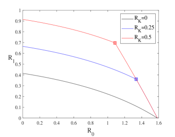
Figure 5: The capacity region of the pure-loss bosonic broadcast channel with confidential messages and key assistance, given the transmissivity $\eta=0.6$, and input constraint $N_{A}=5$. The black, blue, and red lines correspond to the key rates $R_{K}=0$, $R_{K}=0.25$, and $R_{K}=0.5$, respectively. The squares mark a transition (“breaking point”) in each region. For $R_{K}=0.5$ (the red curve), the breaking point is $(R_{0},R_{1})=(1.085,0.697)$, which corresponds to $\beta=0.207$. For low common rates, $R_{0}<1.085$, the shared key is fully used to enhance the communication rates, whereas for higher rates $R_{0}>1.085$, the key is only partially used due to the limitation of Bob’s channel to decode the messages.

III-C Pure-Loss Bosonic Channel

For the pure-loss bosonic broadcast channel, in which the noise mode is in the vacuum state, we determine the capacity region exactly, under the assumption of the minimum output-entropy conjecture. This long-standing conjecture is known to hold in special cases [77]. As mentioned above, the main technical challenge is in the single-letter converse proof, which requires the conjecture. Denote the channel by $\mathcal{L}_{\text{pure-loss}}$.

Conjecture 1 (see [80]).

Let the noise modes $\{\hat{c}_{i}\}_{i=1}^{n}$ be in a product state $\rho_{C^{n}}=|0\rangle\langle 0|^{\otimes n}$ of $n$ vacuum states, and assume that $H(A^{n})_{\rho}=ng(N_{A})$. Then,

$$H(B^{n})_{\rho}\geq ng(\eta N_{A})\,.$$ (52)

Theorem 6.

Assume that Conjecture 1 holds. Then, the capacity region of the pure-loss bosonic broadcast channel with confidential messages is as follows. If $\eta\geq\frac{1}{2}$, then

$$\mathcal{C}(\mathcal{L}_{\text{pure-loss}})=\bigcup_{0\leq\beta\leq 1}\left\{\begin{array}[]{rl}(R_{0},R_{1})\,:\;R_{0}\leq&g((1-\eta)N_{A})-g((1-\eta)\beta N_{A})\\ R_{1}\leq&g(\eta\beta N_{A})-g((1-\eta)\beta N_{A})+R_{K}\\ R_{1}\leq&g(\eta\beta N_{A})\end{array}\right\}\,.$$ (56)

Otherwise, if $\eta<\frac{1}{2}$,

$$\mathcal{C}(\mathcal{L}_{\text{pure-loss}})=\bigcup_{0\leq\beta\leq 1}\left\{\begin{array}[]{rl}(R_{0},R_{1})\,:\;R_{0}\leq&g((1-\eta)N_{A})-g((1-\eta)\beta N_{A})\\ R_{1}\leq&\min\left(g(\eta\beta N_{A})\,,\;R_{K}\right)\end{array}\right\}\,.$$ (59)

The capacity region of the pure-loss bosonic broadcast channel is depicted in Figure 5 for different key values, transmissivity $\eta=0.6$, and input constraint $N_{A}=5$. The black, blue, and red lines correspond to the key rates $R_{K}=0$, $R_{K}=0.25$, and $R_{K}=0.5$, respectively. The squares mark the phase transition (“breaking point”) in each region. For $R_{K}=0.5$ (the red curve), the breaking point is $(R_{0},R_{1})=(1.085,0.697)$, which corresponds to $\beta=0.207$. For low common rates, $R_{0}<1.085$, the shared key is fully used to enhance the communication rates, whereas for higher rates $R_{0}>1.085$, the key is only partially used due to the limitation of Bob’s channel to decode the messages. In general, the breaking point corresponds to the value $\beta_{0}$ such that

$$g((1-\eta)\beta_{0}N_{A})=R_{K}\,.$$ (60)

Consider the first part of Theorem 6. The direct part follows immediately from Theorem 4, by taking $N_{C}\rightarrow 0$. To show the converse part, we combine the arguments of Guha and Shapiro [80] for the pure-loss bosonic channel with the methods of Smith [106] for the degraded wiretap channel. The proof requires the strong minimum output-entropy conjecture. That is, we assume that Conjecture 1 holds.

Moving the converse proof, let Alice and Bob share a random key $k$ uniformly distributed over $[1:2^{nR_{K}}]$. Suppose that Alice chooses $m_{0}$ and $m_{1}$ uniformly at random, and prepares an input state $\rho^{m_{0},m_{1},k}_{A^{n}}$. After Alice sends the system $A^{n}$ through the channel, the output state is $\rho_{B^{n}E^{n}}=\frac{1}{2^{n(R_{0}+R_{1}+R_{K})}}\sum_{m_{0}=1}^{2^{nR_{0}}}\sum_{m_{1}=1}^{2^{nR_{1}}}\sum_{k=1}^{2^{nR_{K}}}\mathcal{L}_{A^{n}\rightarrow B^{n}E^{n}}(\rho^{m_{0},m_{1},k}_{A^{n}})$. Then, Bob and Eve perform decoding POVMs $\Gamma^{m_{0},m_{1}}_{B^{n}|k}$ and $\Xi^{m_{0}}_{E^{n}}$, respectively. Consider a sequence of codes $(\mathcal{F}_{n},\Lambda_{n},\Gamma_{n})$ such that the average probability of error and the leakage tend to zero, hence the error probabilities $\Pr\left(\hat{M}_{0}\neq M_{0}\right)$, $\Pr\left((\hat{M}_{0},\hat{M}_{1})\neq(M_{0},M_{1})\right)$, $\Pr\left(\hat{M}_{1}\neq M_{1}|M_{0}\right)$, are bounded by some $\alpha_{n}$ which tends to zero as $n\rightarrow\infty$. By Fano’s inequality [107], it follows that

$$H(M_{0}|\widetilde{M}_{0})\leq n\varepsilon_{n}$$ (61)

$$H(M_{1}|\hat{M}_{1},M_{0})\leq n\varepsilon_{n}^{\prime}$$ (62)

where $\varepsilon_{n},\varepsilon_{n}^{\prime}$ tend to zero as $n\rightarrow\infty$. Since the leakage tends to zero, we also have

$$I(M_{1};E^{n}|M_{0})_{\rho}\leq n\delta_{n}$$ (63)

where $\delta_{n}$ tends to zero as $n\rightarrow\infty$.

First, we show the following multi-letter upper bounds,

$$R_{0} \leq\frac{1}{n}I(M_{0};E^{n})_{\rho}+\varepsilon_{n}$$ (64)

$$R_{1} \leq\frac{1}{n}H(B^{n}|M_{0},K)_{\rho}+\varepsilon_{n}^{\prime}\,.$$ (65)

$$R_{1} \leq\frac{1}{n}[H(B^{n}|M_{0},K)_{\rho}-H(E^{n}|M_{0},K)_{\rho}]+R_{K}+\delta_{n}+\varepsilon_{n}^{\prime}\,.$$ (66)

Indeed, the common rate is bounded as

$$nR_{0} =H(M_{0})=I(M_{0};\widetilde{M}_{0})_{\rho}+H(M_{0}|\widetilde{M}_{0})$$

$$\leq I(M_{0};\widetilde{M}_{0})_{\rho}+n\varepsilon_{n}$$

$$\leq I(M_{0};E^{n})_{\rho}+n\varepsilon_{n}$$ (67)

where the first inequality follows from (61), and the last inequality follows from the Holevo bound due to data processing inequality (see [105, Theorem 12.1]).

Similarly, the private rate is bounded as

$$nR_{1} \leq I(M_{1};B^{n},K|M_{0})_{\rho}+n\varepsilon_{n}^{\prime}$$

$$=I(M_{1};B^{n}|M_{0},K)_{\rho}+n\varepsilon_{n}^{\prime}$$ (68)

$$\leq H(B^{n}|M_{0},K)_{\rho}+n\varepsilon_{n}^{\prime}$$ (69)

where the equality follows from the statistical independence between the key and the messages, and the last inequality holds since $M_{0}$, $M_{1}$, $K$ are classical. Then, (68) implies that

$$nR_{1} \leq I(M_{1};B^{n}|M_{0},K)_{\rho}-I(M_{1};E^{n}|M_{0})_{\rho}+n\delta_{n}+n\varepsilon_{n}^{\prime}$$ (70)

since we have seen in (63) that $-I(M_{1};E^{n}|M_{0})_{\rho}+n\delta_{n}\geq 0$ because of the leakage requirement. Using the chain rule, we have

$$I(M_{1};E^{n}|M_{0})_{\rho} =I(M_{1};E^{n},K|M_{0})_{\rho}-I(M_{1};K|E^{n},M_{0})_{\rho}$$

$$\geq I(M_{1};E^{n},K|M_{0})_{\rho}-H(K)$$

$$=I(M_{1};E^{n}|M_{0},K)_{\rho}-nR_{K}$$ (71)

where the last two lines follow because the key is classical and uniformly distributed over $[1:2^{nR_{K}}]$. Inserting (71) into the bound on the private rate in (70), we obtain

$$nR_{1} \leq I(M_{1};B^{n}|M_{0},K)_{\rho}-I(M_{1};E^{n}|M_{0},K)_{\rho}+nR_{K}+n(\delta_{n}+\varepsilon_{n}^{\prime})$$ (72)

Now, consider a spectral decomposition of the input state,

$$\rho^{m_{0},m_{1},k}_{A^{n}}=\int p_{Y|M_{0},M_{1},K}(y|m_{0},m_{1},k)|\phi_{A^{n}}^{y,m_{0},m_{1},k}\rangle\langle\phi_{A^{n}}^{y,m_{0},m_{1},k}|\,dy$$ (73)

where $Y$ is an “index” over the continuous ensemble $\{|\phi_{A^{n}}^{y,m_{0},m_{1},k}\rangle\}$, and $p_{Y|M_{0},M_{1},K}(y|m_{0},m_{1},k)$ is a conditional probability density function. Then, augmenting $Y$, we obtain the extended output state,

$$\rho_{YB^{n}E^{n}}^{m_{0},m_{1},k} =\int p_{Y|M_{0},M_{1},K}(y|m_{0},m_{1},k)|y\rangle\langle y|_{Y}\otimes(U^{\mathcal{L}})^{\otimes n}|\phi_{B^{n}E^{n}}^{y,m_{0},m_{1},k}\rangle\langle\phi_{B^{n}E^{n}}^{y,m_{0},m_{1},k}|(U^{\mathcal{L}})^{\otimes n}\,dy$$ (74)

where $U^{\mathcal{L}}$ is the isometry corresponding to the bosonic broadcast channel. By the chain rule,

$$I(M_{1};B^{n}|M_{0},K)_{\rho}-I(M_{1};E^{n}|M_{0},K)_{\rho} =I(M_{1},Y;B^{n}|M_{0},K)_{\rho}-I(M_{1},Y;E^{n}|M_{0},K)_{\rho}$$

$$-[I(Y;B^{n}|M_{0},M_{1},K)_{\rho}-I(Y;E^{n}|M_{0},M_{1},K)_{\rho}]$$

$$\leq I(M_{1},Y;B^{n}|M_{0},K)_{\rho}-I(M_{1},Y;E^{n}|M_{0},K)_{\rho}$$ (75)

where the last inequality holds since the bosonic broadcast channel is degraded and $I(Y;B^{n}|M_{0},M_{1},K)_{\rho}\geq I(Y;E^{n}|M_{0},M_{1},K)_{\rho}$ by the quantum data processing inequality.

Notice that given $M_{j}=m_{j}$, $K=k$, and $Y=y$, the joint state of $(B^{n},E^{n})$ is pure. Therefore, $H(B^{n}|M_{0},M_{1},K,Y)_{\rho}=H(E^{n}|M_{0},M_{1},K,Y)_{\rho}$, and

$$I(M_{1},Y;B^{n}|M_{0},K)_{\rho}-I(M_{1},Y;E^{n}|M_{0},K)_{\rho}=H(B^{n}|M_{0},K)_{\rho}-H(E^{n}|M_{0},K)_{\rho}\,.$$ (76)

Therefore, (72) becomes

$$nR_{1}\leq H(B^{n}|M_{0},K)_{\rho}-H(E^{n}|M_{0},K)_{\rho}+n(R_{K}+\delta_{n}+\varepsilon_{n}^{\prime})\,.$$ (77)

We have thus proved the multi-letter upper bounds (64)-(66), which immediately follow from (67), (69), and (77), respectively, by dividing both sides of each inequality by $n$.

To prove the single-letter converse part, we proceed as follows. Since the thermal state maximizes the quantum entropy over all states with the same first and second moments [108],

$$H(B^{n}|M_{0},K)_{\rho} \leq\sum_{i=1}^{n}H(B_{i}|M_{0},K)_{\rho}$$

$$\leq\sum_{i=1}^{n}g(N_{B_{i}})$$ (78)

where $N_{B_{i}}$ is the mean photon number that corresponds to the $i^{\text{th}}$ output. As $g(\cdot)$ is concave and monotonically increasing,

$$\frac{1}{n}\sum_{i=1}^{n}g(N_{B_{i}}) \leq g\left(\frac{1}{n}\sum_{i=1}^{n}N_{B_{i}}\right)$$

$$\leq g(\eta N_{A})\,.$$ (79)

Together with (78), this implies $\frac{1}{n}H(B^{n}|M_{0},K)_{\rho}\leq g(\eta N_{A})$. Thereby, there exists $0\leq\beta\leq 1$ such that

$$\frac{1}{n}H(B^{n}|M_{0},K)_{\rho}=g(\eta\beta N_{A})\,.$$ (80)

Recall, from Remark 1, that Eve’s degraded state can be obtained as the output of a pure-loss bosonic channel, where the input is Bob’s state, and the transmissivity for this degrading channel is $\eta^{\prime}=\frac{1-\eta}{\eta}$ (see Figure 2). Thereby, assuming Conjecture 1 holds, we can deduce from (80) that

$$\frac{1}{n}H(E^{n}|M_{0},K)_{\rho}\geq g(\eta^{\prime}\cdot\eta\beta N_{A})=g((1-\eta)\beta N_{A})\,.$$ (81)

By similar considerations,

$$\frac{1}{n}H(E^{n})_{\rho}\leq\frac{1}{n}\sum_{i=1}^{n}g(N_{E_{i}})\leq g\left(\frac{1}{n}\sum_{i=1}^{n}N_{E_{i}}\right)\leq g((1-\eta)N_{A})\,.$$ (82)

Thus,

$$R_{0}-\varepsilon_{n} \stackrel{{\scriptstyle\eqref{eq:multiUp1}}}{{\leq}}\frac{1}{n}I(M_{0},K;E^{n})_{\rho}$$

$$=\frac{1}{n}[H(E^{n})_{\rho}-H(E^{n}|M_{0},K)_{\rho}$$

$$\stackrel{{\scriptstyle(\ast)}}{{\leq}}g((1-\eta)N_{A})-g((1-\eta)\beta N_{A})$$ (83)

$$R_{1}-\varepsilon_{n}^{\prime} \stackrel{{\scriptstyle\eqref{eq:multiUp2}}}{{\leq}}\frac{1}{n}H(B^{n}|M_{0},K)_{\rho}$$

$$\stackrel{{\scriptstyle(\ast)}}{{=}}g(\eta\beta N_{A})$$ (85)

and

$$R_{1}-\delta_{n}-\varepsilon_{n}^{\prime} \stackrel{{\scriptstyle\eqref{eq:multiUp3}}}{{\leq}}\frac{1}{n}[H(B^{n}|M_{0},K)_{\rho}-H(E^{n}|M_{0},K)_{\rho}]+R_{K}$$

$$\stackrel{{\scriptstyle(\ast)}}{{\leq}}g(\eta\beta N_{A})-g((1-\eta)\beta N_{A})+R_{K}$$ (86)

where $(\ast)$ follow from (80)-(81). ∎

IV Main Results – Key Agreement

Consider the distillation of a public key and a secret key between Alice, Bob, and Eve, using a correlated state $\omega_{ABE}^{\otimes n}$, as described in Subsection II-D, and illustrated in Figure 4. This source model is rather different compared to the confidential channel model in the previous section. Yet, we will point out the connection between them in Corollary 8, and in particular, the relation to the bosonic broadcast channel.

We characterize the key-agreement capacity region for the case where $A$, $B$, and $E$ have finite dimensions Define a key-rate region,

$$\mathsf{K}(\omega_{ABE})=\bigcup_{\Lambda_{A}\,,\;p_{T_{0},T_{1}|X}}\left\{\begin{array}[]{lrl}(R_{0},R_{1})\,:&R_{0}\leq&\min\left(I(T_{0};B)_{\omega}\,,\;I(T_{0};E)_{\omega}\right)\\ &R_{1}\leq&[I(X;B|T_{0},T_{1})_{\omega}-I(X;E|T_{0},T_{1})_{\omega}]_{+}\end{array}\right\}\,,$$ (89)

where $[x]_{+}=\max(x,0)$, and the union is over the set of POVMs $\Lambda_{A}=\{\Lambda_{A}^{x}\}_{x\in\mathcal{X}}$ and conditional distributions $p_{T_{0},T_{1}|X}$, with

$$\omega_{T_{0}T_{1}XBE}\equiv\sum_{t_{0},t_{1},x}p_{T_{0},T_{1}|X}(t_{0},t_{1}|x)|t_{0}\rangle\langle t_{0}|\otimes|t_{1}\rangle\langle t_{1}|\otimes|x\rangle\langle x|\otimes\mathrm{Tr}_{A}\left((\Lambda_{A}^{x}\otimes\text{1}\otimes\text{1})\omega_{ABE}\right)\,.$$ (90)

Since any measurement can be extended to a projective measurement [105, Section 2.2.8], the auxiliary variables alphabets can be restricted to $|\mathcal{X}|\leq(|\mathcal{H}_{A}||\mathcal{H}_{B}||\mathcal{H}_{E}|)^{4}$, $|\mathcal{T}_{0}|\leq|\mathcal{X}|+3$, and $|\mathcal{T}_{1}|\leq|\mathcal{T}_{0}||\mathcal{X}|$, by the same arguments as in the proof of Lemma 2 in Appendix A. Hence, the formula above is in principle computable.

The key-agreement theorem is given below.

Theorem 7.

The key-agreement capacity region for the distillation of a public key and a secret key from $\omega_{ABE}$ in finite dimensions is given by

$$\mathcal{K}(\omega_{ABC})=\bigcup_{n=1}^{\infty}\frac{1}{n}\mathsf{K}(\omega_{ABC}^{\otimes n})\,.$$ (91)

The proof of Theorem 7 is given in Appendix C. We note that in the multi-letter capacity result, the auxiliary variable $T_{1}$ is not necessary, as can be seen in the converse proof. However, it emerges as a result of the single letterization for special cases, including a classical channel. Although, in the degraded case, $T_{1}$ is not necessary even for a single-letter characterization. We observe the following relation with the broadcast channel with confidential messages.

Corollary 8.

Let $\mathcal{L}_{A\rightarrow BE}$ be a degraded broadcast channel. Then,

$$\bigcup_{\omega_{ABE}\,:\;\omega_{BE}=\mathcal{L}_{A\rightarrow BE}(\omega_{A})}\mathcal{K}(\omega_{ABC})=\lim_{n\rightarrow\infty}\frac{1}{n}\mathcal{R}(\mathcal{L}^{\otimes n})\,,$$ (92)

where $\mathcal{R}(\cdot)$ is as defined in (26). Thus, The capacity region of a degraded broadcast channel $\mathcal{L}_{A\rightarrow BE}$ with confidential messages satisfies

$$\mathcal{C}(\mathcal{L})=\bigcup_{\omega_{ABE}\,:\;\omega_{BE}=\mathcal{L}_{A\rightarrow BE}(\omega_{A})}\mathcal{K}(\omega_{ABC})\,.$$ (93)

Corollary 8 follows from Theorem 7 in a straightforward manner. Indeed, consider the first part of the corollary. Then, the direct part follows by taking $X=T_{1}$. As for the converse part, we note that for a degraded channel, $I(T_{1};B|T_{0})_{\omega}\geq I(T_{1};E|T_{0})_{\omega}$, by the data processing inequality. Thus,

$$I(X;B|T_{0},T_{1})_{\omega}-I(X;E|T_{0},T_{1})_{\omega} \leq I(X;B|T_{0},T_{1})_{\omega}-I(X;E|T_{0},T_{1})_{\omega}+[I(T_{1};B|T_{0})_{\omega}-I(T_{1};E|T_{0})_{\omega}]$$

$$=I(\widetilde{X};B|T_{0})_{\omega}-I(\widetilde{X};E|T_{0})_{\omega}$$ (94)

where we have defined $\widetilde{X}\equiv(X,T_{0})$. The second part of the corollary follows from Theorem 1. Based on this corollary, the key-agreement capacity region is included within the corresponding confidential capacity region without key assistance. In particular, the key-agreement capacity region for thermal states that are associated with a pure-loss bosonic channel is the same as the confidential capacity region in Theorem 6.

V Layered Secrecy

As mentioned in the introduction, the quantum broadcast channel with layered decoding and secrecy is a generalization of the degraded broadcast channel with confidential messages [28, 29, 30]. The model describes a network in which the users have different credentials to access confidential information. Zou et al. [30] give the practical example of an agency WiFi network, in which a user is allowed to receive files up to a certain security clearance but should be kept ignorant of classified files that require a higher security level. As pointed out in [30], the agency can set the channel quality on a clearance basis by assigning more communication resources to users with a higher clearance. As before, we begin with the finite-dimensional case, and then consider the bosonic channel. We will describe a bosonic network with three receivers, where the channel is formed by a serial connection of two beam splitters, as illustrated in Figure 7. By extending the finite-dimension results, we will derive an achievable layered-secrecy region for the pure-loss bosonic broadcast channel.

Consider a channel $\mathcal{L}_{A\rightarrow BE_{1}E_{2}}$ with three receivers, Bob, Eve 1, and Eve 2. The sender, Alice, sends three messages, $m_{0}$, $m_{1}$, and $m_{2}$. The information has different layers of confidentiality. The message $m_{0}$ is a common message that is intended for all three receivers. In the next layer, the confidential message $m_{1}$ is decoded by Bob and Eve 1 but should remain hidden from Eve 2. The confidential message $m_{2}$ is decoded by Bob, while remaining secret from both Eve 1 and Eve 2. Since $m_{0}$ is not secret, we say that it belongs to layer $0$. Similarly, $m_{1}$ and $m_{2}$ are referred to as the layer-1, and layer-2 messages, respectively. It is assumed that the broadcast channel is degraded. That is, there exist degrading channels $\mathcal{D}_{B\rightarrow E_{1}}$ and $\mathcal{G}_{E_{1}\rightarrow E_{2}}$ such that

$$\mathcal{L}_{A\rightarrow E_{1}}=\mathcal{D}_{B\rightarrow E_{1}}\circ\mathcal{L}_{A\rightarrow B}$$ (95)

and

$$\mathcal{L}_{A\rightarrow E_{2}}=\mathcal{G}_{E_{1}\rightarrow E_{2}}\circ\mathcal{L}_{A\rightarrow E_{1}}$$ (96)

where $\mathcal{L}_{A\rightarrow B}$ and $\mathcal{L}_{A\rightarrow E_{j}}$, $j=1,2$, are the marginal channels of the quantum broadcast channel $\mathcal{L}_{A\rightarrow BE_{1}E_{2}}$.

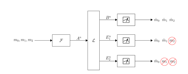
Figure 6: The quantum broadcast channel with layered secrecy.

V-A Layered-Secrecy Coding

We define a layered-secrecy code, where a common message is sent to all receivers, at a rate $R_{0}$, and two confidential messages are sent at rates $R_{1}$ and $R_{2}$

Definition 3.

A $(2^{nR_{0}},2^{nR_{1}},2^{nR_{2}},n)$ layered-secrecy code for the quantum broadcast channel $\mathcal{L}_{A\rightarrow BE_{1}E_{2}}$ consists of the following: three index sets $[1:2^{nR_{j}}]$, for $j=0,1,2$, corresponding to the common message for all users, the confidential message of User 1 and User 2, and the confidential message for User 1 alone, respectively; an encoding map $\mathcal{F}_{A^{n}}$ from the product set $[1:2^{nR_{0}}]\times[1:2^{nR_{1}}]\times[1:2^{nR_{2}}]$ to the input Hilbert space $\mathcal{H}_{A^{n}}$; and three decoding POVMs, $\{\Gamma^{m_{0},m_{1},m_{2}}_{B^{n}}\}$ for Bob and $\{\Xi^{m_{0},m_{1}}_{E_{1}^{n}}\}$, $\{\Upsilon^{m_{0}}_{E_{2}^{n}}\}$ for Eve 1 and Eve 2, respectively. We denote the code by $(\mathcal{F},\Gamma,\Xi,\Upsilon)$.

The communication scheme is depicted in Figure 6. The sender Alice has the system $A^{n}$, and the receivers Bob, Eve 1, and Eve 2 have the systems $B^{n}$, $E_{1}^{n}$, and $E_{2}^{n}$, respectively. Alice chooses a common message $m_{0}\in[1:2^{nR_{0}}]$ that is intended for all users, a layer-1 confidential message $m_{1}\in[1:2^{nR_{1}}]$ for Bob and Eve 1, and a layer-2 confidential message $m_{2}\in[1:2^{nR_{2}}]$, all drawn uniformly at random. She encodes the messages by applying the encoding map $\mathcal{F}_{A^{n}}$ which results in an input state $\rho^{m_{0},m_{1},m_{2}}_{A^{n}}=\mathcal{F}_{A^{n}}(m_{0},m_{1},m_{2})$, and transmits the system $A^{n}$ over $n$ channel uses of $\mathcal{L}_{A\rightarrow BE_{1}E_{2}}$. Hence, the output state is

$$\rho^{m_{0},m_{1},m_{2}}_{B^{n}E_{1}^{n}E_{2}^{n}}=\mathcal{L}^{\otimes n}(\rho^{m_{0},m_{1},m_{2}}_{A^{n}})\,.$$ (97)

Eve 2 receives the channel output system $E_{2}^{n}$, and performs a measurement with the POVM $\{\Upsilon^{m_{0}}_{E_{2}^{n}}\}$. From the measurement outcome, she obtains an estimate of the common message $\breve{m}_{0}\in[1:2^{nR_{0}}]$. Similarly, Eve 1 finds an estimate of the message pair $(\widetilde{m}_{0},\widetilde{m}_{1})\in[1:2^{nR_{0}}]\times[1:2^{nR_{1}}]$ by performing a POVM $\{\Xi^{m_{0},m_{1}}_{E_{2}^{n}}\}$ on the output system $E_{1}^{n}$. Bob estimates all three messages by applying $\{\Gamma^{m_{0},m_{1},m_{2}}_{B^{n}}\}$ on $B^{n}$.

The performance of the layered-secrecy code is measured in terms of the probability of decoding error and the amount of confidential information that is leaked to the non-intended receivers. The conditional probability of error of the code, given that the message pair $(m_{0},m_{1},m_{2})$ was sent, is given by

$$P_{e|m_{0},m_{1},m_{2}}^{(n)}(\mathcal{F},\Gamma,\Xi,\Upsilon) =1-\mathrm{Tr}[(\Gamma^{m_{0},m_{1},m_{2}}_{B^{n}}\otimes\Xi^{m_{0},m_{1}}_{E_{1}^{n}}\otimes\Upsilon^{m_{0}}_{E_{2}^{n}})\rho^{m_{0},m_{1},m_{2}}_{B^{n}E_{1}^{n}E_{2}^{n}}]\,.$$ (98)

The layer-1 confidential message $m_{1}$ needs to remain secret from Eve 2, and the layer-2 confidential message $m_{2}$ needs to remain secret from both Eve 1 and Eve 2. Thereby, the leakage rates of the code $(\mathcal{F},\Gamma,\Xi,\Upsilon)$ are defined as

$$s_{1}^{(n)}(\mathcal{F}) \triangleq I(M_{1};E_{2}^{n}|M_{0})_{\rho}$$ (99)

$$s_{2}^{(n)}(\mathcal{F}) \triangleq I(M_{2};E_{1}^{n},E_{2}^{n}|M_{0})_{\rho}$$ (100)

where $M_{j}$ is a classical random variable that is uniformly distributed over the corresponding message index set, $[1:2^{nR_{j}}]$, for $j=1,2$.

A $(2^{nR_{0}},2^{nR_{1}},2^{nR_{2}},n,\varepsilon,\delta)$ confidential code satisfies $\frac{1}{2^{n(R_{0}+R_{1})}}\sum_{m_{0},m_{1}}P_{e|m_{0},m_{1}}^{(n)}(\mathcal{F},\Gamma,\Xi)\leq\varepsilon$ and $s^{(n)}_{j}(\mathcal{F})\leq\delta$ for $j=0,1$. A rate tuple $(R_{0},R_{1},R_{2})$, where $R_{j}\geq 0$, $j=0,1,2$, is achievable if for every $\varepsilon,\delta>0$ and sufficiently large $n$, there exists a $(2^{nR_{0}},2^{nR_{1}},2^{nR_{2}},n,\varepsilon,\delta)$ layered-secrecy code. The operational layered-secrecy capacity region $\mathcal{C}_{\text{LS}}(\mathcal{L})$ of the quantum broadcast channel $\mathcal{L}_{A\rightarrow BE_{1}E_{2}}$ is defined as the set of achievable tuples $(R_{0},R_{1},R_{2})$ with layered secrecy.

As before, in the bosonic case, it is assumed that the encoder uses a coherent state protocol with an input constraint. Specifically, the input state is a coherent state $|f(m_{0},m_{1},m_{2})\rangle$, where the encoding function, $f:[1:2^{nR_{0}}]\times[1:2^{nR_{1}}]\times[1:2^{nR_{2}}]\to\mathbb{C}^{n}$, satisfies $\frac{1}{n}\sum_{i=1}^{n}|f_{i}(m_{0},m_{1},m_{2})|^{2}\leq N_{A}$.

Remark 11.

Here, the index $j$ of the rate $R_{j}$ corresponds to the secrecy layer. The common message rate $R_{0}$ is associated with non-secret information, i.e., layer $0$. The confidential message rate $R_{1}$ is associated with layer-1 information, which is secret from one of the users, namely, Eve 2. In the WiFi network example mentioned above, this means that Bob and Eve 1 have a higher clearance to access classified information. The confidential message rate $R_{2}$ is associated with a highly classified layer-2 information, and Bob is the only one who has the authority to access this information. As presented by Zou et al. [30], the model can be further generalized to $N$ receivers with $N$ secrecy layers, where User $j$ should only decode the messages $m_{0},\ldots,m_{N-j}$, which belong to the $j^{\text{th}}$ layer.

Remark 12.

Removing Eve 1 (say, $E_{1}$ has a single dimension), the model reduces to the quantum broadcast channel with confidential messages, which in turn generalizes the wiretap channel (see Remark 3). In the case of the broadcast channel with confidential messages, we only have layer-0 and layer-2 messages, whereas the layer-1 rate is $R_{1}=0$.

Remark 13.

As pointed out in Remark 4, if one considers the transmission of quantum states, instead of classical information, then secrecy is guaranteed by default by the no-cloning theorem. As the quantum “message” state cannot be recovered by more than one receiver, this means that the layer-0 and layer-1 quantum rates (in units of qubits per channel use) must be zero, and we can only have layer-2 communication.

V-B Main Results – Finite Dimensions

Consider the quantum degraded broadcast channel $\mathcal{L}_{A\rightarrow BE_{1}E_{2}}$ with layered secrecy. We obtain a regularized formula for the capacity region in this setting. Define

$$\mathcal{R}_{\text{LS}}(\mathcal{L})=\bigcup_{p_{X_{0},X_{1},X_{2}}\,,\;\varphi_{A}^{x_{0},x_{1},x_{2}}}\left\{\begin{array}[]{lrl}(R_{0},R_{1},R_{2})\,:&R_{0}\leq&I(X_{0};E_{2})_{\rho}\\ &R_{1}\leq&[I(X_{1};E_{1}|X_{0})_{\rho}-I(X_{1};E_{2}|X_{0})_{\rho}]_{+}\\ &R_{2}\leq&[I(X_{2};B|X_{0},X_{1})_{\rho}-I(X_{2};E_{1}E_{2}|X_{0},X_{1})_{\rho}]_{+}\end{array}\right\}\,,$$ (104)

where the union is over the distribution of the auxiliary random variables $X_{0}$, $X_{1}$, $X_{2}$ and the collections of quantum states $\{\varphi_{A}^{x_{0},x_{1},x_{2}}\}$, with

$$\rho_{X_{0}X_{1}X_{2}BE_{1}E_{2}}=\sum_{x_{0},x_{1},x_{2}}p_{X_{0},X_{1},X_{2}}(x_{0},x_{1},x_{2})\mathcal{L}_{A\rightarrow BE_{1}E_{2}}(\varphi_{A}^{x_{0},x_{1},x_{2}})\,.$$ (105)

Theorem 9.

The layered-secrecy capacity region of the quantum degraded broadcast channel $\mathcal{L}_{A\rightarrow BE_{1}E_{2}}$ in finite dimensions is given by

$$\mathcal{C}_{\text{LS}}(\mathcal{L})=\bigcup_{n=1}^{\infty}\frac{1}{n}\mathcal{R}_{\text{LS}}(\mathcal{L}^{\otimes n})\,.$$ (106)

The proof of Theorem 9 is given in Appendix D.

Remark 14.

Given a classical degraded broadcast channel $W_{YZ_{1}Z_{2}|X}$, the bound on the top-secret rate $R_{2}$ in (104) can be simplified. In particular, we can choose $X_{2}$ to be the channel input, i.e., $X_{2}=X$. Furthermore, the auxiliary random variables can be chosen such that $X_{0}\leavevmode\hbox to9.01pt{\vbox to4.71pt{\text{[drawing]}}}X_{1}\leavevmode\hbox to9.01pt{\vbox to4.71pt{\text{[drawing]}}}X\leavevmode\hbox to9.01pt{\vbox to4.71pt{\text{[drawing]}}}Y\leavevmode\hbox to9.01pt{\vbox to4.71pt{\text{[drawing]}}}Z_{1}\leavevmode\hbox to9.01pt{\vbox to4.71pt{\text{[drawing]}}}Z_{2}$ form a Markov chain, given a physically degraded broadcast channel. That is, the joint distribution of those variables can be expressed as

$$p_{X_{0}X_{1}XYZ_{1}Z_{2}}(x_{0},x_{1},x,y,z_{1},z_{2})=p_{X_{0}}(x_{0})p_{X_{1}|X_{0}}(x_{1}|x_{0})p_{X|X_{1}}(x|x_{1})W_{Y|X}(y|x)D_{1}(z_{1}|y)D_{2}(z_{2}|z_{1})\,,$$ (107)

for some input distributions $p_{X_{0}}$, $p_{X_{1}|X_{0}}$, and $p_{X|X_{1}}$, and degrading channels $D_{j}$, for $j=1,2$. In this case, we have

$$I(X;Y|X_{0},X_{1})-I(X;Z_{1}Z_{2}|X_{0},X_{1})=I(X;Y|X_{1})-I(X;Z_{1}|X_{1})\,.$$ (108)

The last equation also holds for a stochastically-degraded classical channel [45]. On the other hand, in the quantum case, the identity $H(B|E_{1}E_{2})_{\rho}=H(B|E_{1})_{\rho}$ holds if only if $B\leavevmode\hbox to9.01pt{\vbox to4.71pt{\text{[drawing]}}}E_{1}\leavevmode\hbox to9.01pt{\vbox to4.71pt{\text{[drawing]}}}E_{2}$ form a quantum Markov chain, which is not guaranteed in our model. A quantum Markov chain is defined as follows. The quantum systems $A\leavevmode\hbox to9.01pt{\vbox to4.71pt{\text{[drawing]}}}B\leavevmode\hbox to9.01pt{\vbox to4.71pt{\text{[drawing]}}}C$ form a Markov chain if and only if there exists a recovery channel $\mathscr{R}_{B\rightarrow BC}$ such that $\rho_{ABC}=(\mathrm{id}_{A}\otimes\mathscr{R}_{B\rightarrow BC})(\rho_{AB})$ [109]. However, as pointed out in [69], the fact that the quantum broadcast channel is degraded does not imply that $B\leavevmode\hbox to9.01pt{\vbox to4.71pt{\text{[drawing]}}}E_{1}\leavevmode\hbox to9.01pt{\vbox to4.71pt{\text{[drawing]}}}E_{2}$ form a quantum Markov chain.

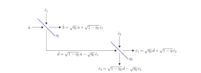
Figure 7: The 3-receiver bosonic broadcast channel with layered secrecy.

V-C Main Results – Bosonic Channel

In this section, we consider layered secrecy for the pure-loss bosonic broadcast channel, specified by

$$\hat{b} =\sqrt{\eta_{1}}\,\hat{a}+\sqrt{1-\eta_{1}}\,\hat{c}_{1}$$ (109)

$$\hat{d} =\sqrt{1-\eta_{1}}\,\hat{a}-\sqrt{\eta_{1}}\,\hat{c}_{1}$$ (110)

and

$$\hat{e}_{1} =\sqrt{\eta_{2}}\,\hat{d}+\sqrt{1-\eta_{2}}\,\hat{c}_{2}$$ (111)

$$\hat{e}_{2} =\sqrt{1-\eta_{2}}\,\hat{d}-\sqrt{\eta_{2}}\,\hat{c}_{2}$$ (112)

where $\hat{c}_{j}$ is associated with the environment noise and the parameter $\eta_{j}$ is the transmissivity, $\frac{1}{2}\leq\eta_{j}\leq 1$, which depends on the length of the optical fiber and its absorption length, for $j=1,2$. The relation above corresponds to a concatenation of two beam splitters. It is assumed that the noise modes $\hat{c}_{1}$ and $\hat{c}_{2}$ are uncorrelated and in the vacuum state. As illustrated in Figure 7, the 3-receiver pure-loss bosonic broadcast channel corresponds to the operation of two beam splitters.

We determine the capacity region. Denote the channel by $\mathcal{L}_{\text{pure-loss}}$.

Our result relies on the long-standing strong minimum output-entropy conjecture, Conjecture 1.

Theorem 10.

Assume that Conjecture 1 holds. Then, the layered-secrecy capacity region of the pure-loss bosonic broadcast channel is bounded by

$$\mathcal{C}_{\text{LS}}(\mathcal{L}_{\text{pure-loss}})\supseteq\bigcup_{\begin{subarray}{c}\beta_{1},\beta_{2}\geq 0\,,\\ \beta_{1}+\beta_{2}\leq 1\end{subarray}}\left\{\begin{array}[]{rl}(R_{0},R_{1})\,:\;R_{0}\leq&g\big{(}(1-\eta_{1})(1-\eta_{2})N_{A}\big{)}-g\big{(}(\beta_{1}+\beta_{2})(1-\eta_{1})(1-\eta_{2})N_{A}\big{)}\\ R_{1}\leq&g\big{(}(\beta_{1}+\beta_{2})\eta_{2}(1-\eta_{1})N_{A}\big{)}-g\big{(}\beta_{2}\eta_{2}(1-\eta_{1})N_{A}\big{)}\\ &-[g\big{(}(\beta_{1}+\beta_{2})(1-\eta_{2})(1-\eta_{1})N_{A}\big{)}-g(\beta_{2}(1-\eta_{2})(1-\eta_{1})N_{A}\big{)}]\\ R_{2}\leq&g\big{(}\eta_{1}\beta_{2}N_{A}\big{)}-g\big{(}(1-\eta_{1})\beta_{2}N_{A}\big{)}\end{array}\right\}\,.$$ (117)

To show Theorem 10, we extend the finite-dimension result in Theorem 9 to the bosonic channel with infinite-dimension Hilbert spaces based on the discretization limiting argument by Guha et al. [81] (see also Subsection VI-A for further expalanation). If one ignores the input constraint, then based on Theorem 9, the region $\mathcal{R}_{\text{LS}}(\mathcal{L}_{\text{pure-loss}})$ is achievable, i.e., $\mathcal{C}_{\text{LS}}(\mathcal{L}_{\text{lossy}})\supseteq\mathcal{R}_{\text{LS}}(\mathcal{L}_{\text{lossy}})$. Thus, we obtain the following inner bound,

$$\mathcal{C}_{\text{LS}}(\mathcal{L}_{\text{lossy}})\supseteq\left\{\begin{array}[]{rl}(R_{0},R_{1})\,:\;R_{0}\leq&I(X_{0};E_{2})_{\rho}\\ R_{1}\leq&I(X_{1};E_{1}|X_{0})_{\rho}-I(X_{1};E_{2}|X_{0})_{\rho}\\ R_{2}\leq&I(X_{2};B|X_{0},X_{1})_{\rho}-I(X_{2};E_{1}E_{2}|X_{0},X_{1})_{\rho}\end{array}\right\}\,,$$ (121)

where the auxiliary variables $X_{j}$ can be chosen arbitrarily. Given the input constraint, we need to add the restriction $\mathbb{E}(|X_{2}|^{2})\leq N_{A}$.

Then, set the input to be a coherent state with $X_{1}=X_{0}+Q_{1}$ and $X_{2}=X_{1}+Q_{2}$, where $X_{j}$ and $Q_{j}$ are independent complex Gaussian random variables,

$$X_{0} \sim\mathcal{N}_{\mathbb{C}}(0,(1-\beta_{1}-\beta_{2})\frac{N_{A}}{2})$$ (122)

$$Q_{j} \sim\mathcal{N}_{\mathbb{C}}(0,\beta_{j}\frac{N_{A}}{2})$$ (123)

for some $\beta_{j}\in[0,1]$, $j=1,2$. Then, $X_{1}$ and $X_{2}$ are distributed according to

$$X_{1} \sim\mathcal{N}_{\mathbb{C}}(0,\frac{(1-\beta_{2})N_{A}}{2})$$ (124)

$$X_{2} \sim\mathcal{N}_{\mathbb{C}}(0,\frac{N_{A}}{2})\,.$$ (125)

Consider the first beam splitter. Since the conditional distribution of $X_{2}$ given $X_{1}=x_{1}$, $X_{0}=x_{0}$ is $\sim\mathcal{N}_{\mathbb{C}}(0,\beta_{2}\frac{N_{A}}{2})$, the mutual informations corresponding to each output are given by

$$I(X_{2};B|X_{0},X_{1}) =H(B|X_{0},X_{1})_{\rho}=g(\eta_{1}\beta_{2}N_{A})$$ (126)

$$I(X_{2};E_{1}E_{2}|X_{0},X_{1}) =H(D|X_{0},X_{1})=g\big{(}(1-\eta_{1})\beta_{2}N_{A}\big{)}$$ (127)

where the first equality in (127) holds since the broadcast channel from $D$ to $E_{1}E_{2}$ is isometric.

As for the second beam splitter, observe that the mean photon number of the input is $N_{D}=(1-\eta_{1})N_{A}$. Hence, the entropies corresponding to each output are given by

$$H(E_{1})_{\rho} =g(\eta_{2}N_{D})=g\big{(}\eta_{2}(1-\eta_{1})N_{A}\big{)}$$ (128)

$$H(E_{1}|X_{0})_{\rho} =g\big{(}\eta_{2}(\beta_{1}+\beta_{2})N_{D}\big{)}=g\big{(}\eta_{2}(\beta_{1}+\beta_{2})(1-\eta_{1})N_{A}\big{)}$$ (129)

$$H(E_{1}|X_{0},X_{1})_{\rho} =g(\eta_{2}\beta_{2}N_{D})=g\big{(}\eta_{2}\beta_{2}(1-\eta_{1})N_{A}\big{)}$$ (130)

and

$$H(E_{2})_{\rho} =g\big{(}(1-\eta_{2})N_{D}\big{)}=g\big{(}(1-\eta_{2})(1-\eta_{1})N_{A}\big{)}$$ (131)

$$H(E_{2}|X_{0})_{\rho} =g\big{(}(1-\eta_{2})(\beta_{1}+\beta_{2})N_{D}\big{)}=g\big{(}(1-\eta_{2})(\beta_{1}+\beta_{2})(1-\eta_{1})N_{A}\big{)}$$ (132)

$$H(E_{2}|X_{0},X_{1})_{\rho} =g\big{(}(1-\eta_{2})\beta_{2}N_{D}\big{)}=g\big{(}(1-\eta_{2})\beta_{2}(1-\eta_{1})N_{A}\big{)}$$ (133)

Thus,

$$I(X_{0};E_{2})_{\rho} =H(E_{2})_{\rho}-H(E_{2}|X_{0})_{\rho}=g\big{(}(1-\eta_{2})(1-\eta_{1})N_{A}\big{)}-g\big{(}(1-\eta_{2})(\beta_{1}+\beta_{2})(1-\eta_{1})N_{A}\big{)}$$ (134)

$$I(X_{1};E_{1}|X_{0})_{\rho} =H(E_{1}|X_{0})_{\rho}-H(E_{1}|X_{0},X_{1})_{\rho}=g\big{(}\eta_{2}(\beta_{1}+\beta_{2})(1-\eta_{1})N_{A}\big{)}-g\big{(}\eta_{2}\beta_{2}(1-\eta_{1})N_{A}\big{)}$$ (135)

$$I(X_{1};E_{2}|X_{0})_{\rho} =H(E_{1}|X_{0})_{\rho}-H(E_{1}|X_{0},X_{1})_{\rho}=g\big{(}(1-\eta_{2})(\beta_{1}+\beta_{2})(1-\eta_{1})N_{A}\big{)}-g\big{(}(1-\eta_{2})\beta_{2}(1-\eta_{1})N_{A}\big{)}$$ (136)

This completes the achievability proof.

VI Discussion

VI-A Discretization

Many capacity theorems for Gaussian channels, in both classical and quantum information theory, are derived by extending the finite-dimension results to the continuous infinite-dimension Gaussian channel [45]. This requires a discretization limiting argument, as e.g., in [81]. This approach is often more convenient than devising a coding scheme and perform the analysis “from scratch”. Yet, such a proof is less transparent and may give less insight for the design of practical error-correction codes (see also discussion in [110]).

The most common discretization approach is based on the following operational argument. Consider a classical memoryless channel $W_{Y|X}$, with continuous input $X$ and output $Y$. We can construct a codebook while restricting ourselves to discrete values, in $\{-L\delta,-(L-1)\delta,\ldots,-\delta,0,\delta,\ldots,(L-1)\delta,L\delta\}$, and the decoder can also discretize the received signal, with an arbitrarily small discretization step $\delta>0$ and arbitrarily large $L>0$. In this manner, we are effectively coding over a finite-dimension channel, with input $X_{\delta}$ and ouput $Y_{\delta}$ over finite alphabets. Thus, by the finite-dimension capacity result, for every input distribution $p_{X_{\delta}}$, a rate $R<I(X_{\delta};Y_{\delta})-\varepsilon$ is achievable, for arbitrarily small $\varepsilon>0$. The achievability proof can then be completed by analyzing the limit of the mutual information $I(X_{\delta};Y_{\delta})$ as $\delta$ tends to zero. A similar argument can be applied for the bosonic channel, where the input is restricted to coherent states of discretized values and the output dimension is restricted by the decoding measurement. For basic channel networks, the Gaussian capacity result can be obtained directly. However, in adversarial models, such as the wiretap channel, this approach may become tricky. In particular, a straightforward application will force the eavesdropper to discretize her signal. Clearly, this does not make sense operationally.

An alternative discretization approach, which can be applied to adversarial models as well, is based on continuity arguments. In particular, we can view the operational capacity $C(W)$ as an unknown functional of the probability measure $W_{Y|X}$, which may have either finite or infinite dimensions. Then, if $W_{Y|X}$ is a Gaussian channel, then we can define a sequence of discretized channels $\{\bar{W}^{\delta_{k}}_{Y|X}\}_{k\geq 1}$, where $\delta_{1},\delta_{2},\ldots$ converges to zero uniformly. Since the Gaussian distribution is continuous and smooth, the sequence of probability measures $\{\bar{W}^{\delta_{k}}_{Y|X}\}_{k\geq 1}$ converges to the Gaussian probability measure $W_{Y|X}$. Furthermore, we have

$$\lim_{\delta\to 0}\bar{W}^{\delta}_{Y|X}=W_{Y|X}\,.$$ (137)

This follows from the observation that in the Gaussian case, the discretized measure $W^{\delta}_{Y|X}$ is continuous in $\delta$. Now, given a channel $\bar{W}_{Y|X}$ in finite dimensions, let $\mathsf{R}(\bar{W})$ denote the capacity formula. Then, based on the finite-dimension capacity theorem, the capacity formula $\mathsf{R}(\bar{W})$ of a channel $\bar{W}$ in finite dimensions is continuous in the channel parameters, since the mutual information $I(X;Y)$ is a continuous functional in the joint distribution $p_{X,Y}$, which can be extended to quantum channels as well [111]. The finite-dimension capacity theorem states that the operational capacity and the capacity formula are identical, i.e., $C(\bar{W})=\mathsf{R}(\bar{W})$, for a finite-dimension channel $\bar{W}$. This, in turn, implies that the operational capacity $C(\bar{W})$ is also a continuous functional.

In general, a composite of two continuous functions $f:\mathcal{A}\to\mathcal{B}$ and $g:\mathcal{B}\to\mathbb{R}$ satisfies $\lim_{x\rightarrow x_{0}}f(g(x))=f(\lim_{x\rightarrow x_{0}}g(x))$, for every $x_{0}\in\mathcal{A}$ such that those limits exist, and this property can also be extended to limits of sequences. Thereby, the limit of the capacities of the discretized channels converges to the capacity of the Gaussian channel. Specifically,

$$C(W) \stackrel{{\scriptstyle(a)}}{{=}}C\left(\lim_{\delta\rightarrow 0}\bar{W}^{\delta}\right)$$

$$\stackrel{{\scriptstyle(b)}}{{=}}\lim_{\delta\rightarrow 0}C\left(\bar{W}^{\delta}\right)$$

$$\stackrel{{\scriptstyle(c)}}{{=}}\lim_{\delta\rightarrow 0}\mathsf{R}\left(\bar{W}^{\delta}\right)$$

$$\stackrel{{\scriptstyle(d)}}{{=}}\mathsf{R}\left(\lim_{\delta\rightarrow 0}\bar{W}^{\delta}\right)$$

$$\stackrel{{\scriptstyle(a)}}{{=}}\mathsf{R}(W)\,,$$ (138)

where $(a)$ follows from the convergence property in (137), $(b)$ holds by the continuity of the operational capacity and the Gaussian channel measure, $(c)$ follows from the finite-dimension capacity theorem, and $(d)$ from the continuity of the mutual-information formula and the Gaussian channel measure. We note that we have repeatedly used the continuity of the channel distribution and the convergence of the discretized sequence, for a discretization of our choice. Thus, the arguments above are not suitable for a general channel measure. The advantage of this discretization approach, using continuity arguments, is that it yields the capacity of Gaussian and bosonic channels in a direct manner, even with security requirements. As before, a similar argument can be applied for the bosonic channel, where the input is now restricted to discretized-value coherent states and the output dimension is restricted by the decoding measurement.

The disadvantage of this approach is that it removes the operational meaning of the capacity and error-correction codes from consideration, and turns the problem into a calculus exercise. This makes it difficult to gain insight on the design of coding techniques for Gaussian channels.

VI-B Strong Minimum Output-Entropy Conjecture

The converse part of our result on the pure-loss bosonic broadcast channel with confidential messages relies on the strong minimum output-entropy conjecture. In the single-user case, the conjecture is not required. As previously mentioned, the single-user wiretap channel can be obtained from the broadcast model with confidential messages by restricting the common message rate to $R_{0}=0$ (see Remark 3). That is, in the wiretap setting, Eve eavesdrops on the confidential message of Bob, and she is not required to decode any messages. In the special case of an isometric wiretap channel $\mathcal{U}_{A\to BE}$, Eve’s system is interpreted as Bob’s environment, and the secrecy capacity of the wiretap channel is referred to as the private capacity of the main channel $\mathcal{L}_{A\rightarrow B}$ (see Remark 8). Denote the private capacity by $C_{\text{P}}(\mathcal{L})$. For a degradable isometric channel in finite dimension, the private capacity equals the quantum capacity, and it is given by

$$C_{\text{P}}(\mathcal{L})=\max_{|\phi_{AA^{\prime}}\rangle}[H(B)_{\rho}-H(E)_{\rho}]$$ (139)

with $\rho_{A^{\prime}BE}\equiv(\mathcal{U}_{A\to BE}\otimes\mathrm{id})(\phi_{AA^{\prime}})$ (see [60, Theorem 13.6.2]). As Wilde and Qi established in [112], in the bosonic case under input constraint $N_{A}$, the maximum is achieved for a thermal state $\tau(N_{A})$ (see Theorem 6 therein). Hence, the private capacity of the pure-loss bosonic channel is given by

$$C_{P}(\mathcal{L}_{\text{pure-loss}})=[g(\eta N_{A})-g((1-\eta)N_{A})]_{+}\,.$$ (140)

Wilde and Qi’s derivation [112] for this property is based on the following argument. Based on the monotonicity of the divergence with respect to quantum channels, we have $D(\rho_{B}||\tau(\eta N_{A}))\geq D(\rho_{E}||\tau((1-\eta)N_{A}))$, as Eve’s channel is degraded with respect to Bob’s channel. This, in turn, can be written as

$$H(B)_{\rho}-H(E)_{\rho}\leq\mathrm{Tr}(\rho_{E}\log\tau((1-\eta)N_{A}))-\mathrm{Tr}(\rho_{B}\log\tau(\eta N_{A}))\,.$$ (141)

Plugging a thermal state, $\tau(N)=\frac{e^{-NG}}{\mathrm{Tr}(e^{-NG})}$ where $G$ is a Gibbs observable, into the RHS, we obtain

$$\mathrm{Tr}(\rho_{E}\log\tau((1-\eta)N_{A}))-\mathrm{Tr}(\rho_{B}\log\tau(\eta N_{A})) =\log\frac{\mathrm{Tr}(e^{-N_{A}G})}{\mathrm{Tr}(e^{-(1-\eta)N_{A}G})}-\mathrm{Tr}(G\rho_{E})+\mathrm{Tr}(G\rho_{B})$$

$$\leq\log\frac{\mathrm{Tr}(e^{-N_{A}G})}{\mathrm{Tr}(e^{-(1-\eta)N_{A}G})}-(1-\eta)N_{A}+\eta N_{A}$$ (142)

since $\mathrm{Tr}(G\rho_{B})\leq\eta N_{A}$ and $\mathrm{Tr}(G\rho_{E})\geq\eta N_{A}$. The proof follows since the inequalities above are saturated for a thermal input state $\rho_{A}=\tau(N_{A})$. Unfortunately, this technique does not seem to yield the desired result for a broadcast channel.

The minimum output-entropy conjecture, Conjecture 1, is known to hold in special cases [113, Remark 2]. In particular, the conjecture was proved to hold for $n=1$. This weak version of the minimum output-entropy property was established by De Palma et al. [114], in 2017, using Lagrange multiplier techniques (see also [115]). However, as pointed out in [114, Sec. V], this is insufficient for the converse proof of the bosonic broadcast channel, which requires the strong minimum output-entropy conjecture.

VII Acknowledgments

Uzi Pereg and Roberto Ferrara were supported by the German Bundesministerium für Bildung und Forschung (BMBF) through Grant n. 16KIS0856. Matthieu Bloch was supported by the American National Science Foundation (NSF) through Grant n. 1955401. Pereg was also supported by the Israel CHE Fellowship for Quantum Science and Technology.

Appendix A Proof of Lemma 2

Consider the region $\mathsf{C}_{\text{k-a}}(\mathcal{L})$ as defined in (32).

A-A Cardinality Bounds

To bound the alphabet size of the random variables $T$ and $X$, we use the Fenchel-Eggleston-Carathéodory lemma [116] and arguments similar to [117]. Let

$$N_{0}= |\mathcal{H}_{A}|^{4}+3$$ (143)

$$N_{1}= |\mathcal{T}|(|\mathcal{H}_{A}|^{4}+2)\,.$$ (144)

First, fix $p_{X|T}(x|t)$, and consider the ensemble $\{p_{T}(t)p_{X|T}(x|t)\,,\varphi_{A}^{t,x}\}$. Every mixed state $\varphi_{A}$ has a unique parametric representation $u(\varphi_{A})$ of dimension $|\mathcal{H}_{A}|^{4}-1$, since the corresponding density matrix has $|\mathcal{H}_{A}|^{2}$ complex entries and the constraint $\mathrm{Tr}(\varphi_{A})=1$. Then, define a map $f_{0}:\mathcal{X}\rightarrow\mathbb{R}^{N_{0}}$ by

$$f_{0}(t)=\left(u(\rho_{A}^{t})\,,\;H(B|T=t)_{\rho}\,,\;H(E|T=t)_{\rho}\,,\;H(B|X,T=t)_{\rho}\,,\;H(E|X,T=t)_{\rho}\right)$$ (145)

where $\rho_{A}^{t}=\sum_{x}p_{X|T}(x|t)\theta_{A}^{t,x}$. The map $f_{0}$ can be extended to probability distributions as follows,

$$F_{0}\,:\;p_{T}\mapsto\sum_{t\in\mathcal{T}}p_{T}(t)f_{0}(t)=\left(u(\rho_{A})\,,\;H(B|T)_{\rho}\,,\;H(E|T)_{\rho}\,,\;H(B|X,T)_{\rho}\,,\;H(E|X,T)_{\rho}\right)$$ (146)

where $\rho_{A}=\sum_{t}p_{T}(t)\rho_{A}^{t}$. According to the Fenchel-Eggleston-Carathéodory lemma [116], any point in the convex closure of a connected compact set within $\mathbb{R}^{d}$ belongs to the convex hull of $d$ points in the set. Since the map $F_{0}$ is linear, it maps the set of distributions on $\mathcal{T}$ to a connected compact set in $\mathbb{R}^{N_{0}}$. Thus, for every $p_{T}$, there exists a probability distribution $p_{\bar{T}}$ on a subset $\overline{\mathcal{T}}\subseteq\mathcal{T}$ of size $N_{0}$, such that $F_{0}(p_{\bar{T}})=F_{0}(p_{T})$. We deduce that the alphabet size can be restricted to $|\mathcal{T}|\leq N_{0}$, while preserving $\rho_{A}$ and $\rho_{BE}\equiv\mathcal{L}_{A\rightarrow BE}(\rho_{A})$; $I(T;B)_{\rho}=H(B)_{\rho}-H(B|T)_{\rho}$, $I(X;B|T)_{\rho}=H(B|T)_{\rho}-H(B|X,T)_{\rho}$; and similarly, $I(T;E)_{\rho}$ and $I(X;E|T)_{\rho}$.

We move to the alphabet size of $X$. We keep $\mathcal{T}$ and $p_{T}$ fixed. Then, define the map $f_{1}^{(t)}:\mathcal{X}\rightarrow\mathbb{R}^{N_{1}}$ by

$$f^{(t)}_{1}(x)= \left(p_{T}(t)\,,\;u(\varphi_{A}^{t,x})\,,\;H(B|X=x,T=t)_{\rho}\,,\;H(E|X=x,T=t)_{\rho}\right)$$ (147)

for $t\in\mathcal{T}$. Now, the extended map is

$$F^{(t)}_{1}\,:\;p_{X|T=t}\mapsto\sum_{x\in\mathcal{X}}p_{X|T}(x|t)f^{(t)}_{1}(x)=\left(p_{T}(t)\,,\;u(\rho_{A}^{t})\,,\;H(B|X,T=t)_{\rho}\,,\;H(E|X,T=t)_{\rho}\}_{t\in\mathcal{T}}\right)\,.$$ (148)

By the Fenchel-Eggleston-Carathéodory lemma [116], for every $p_{X|T}$, there exists $p_{\bar{X}|T}$ on a subset $\overline{\mathcal{X}}\subseteq\mathcal{X}$ of size $N_{1}$, such that $F_{1}^{(t)}(p_{\bar{X}|T=t})=F_{1}^{(t)}(p_{X|T=t})$ for all $t\in\mathcal{T}$. Thus, we can restrict the alphabet size to $|\mathcal{X}|\leq N_{1}$, while preserving $\rho_{A}^{t}$, $H(B|T)_{\rho}=\sum_{t}H(B|T)_{\mathcal{L}^{(1)}(\sigma_{A}^{t})}$ and similarly $H(B|T)_{\rho}$; $\rho_{A}$, $\rho_{B,E}$, $I(X;B|T)_{\rho}$, and $I(X;E|T)_{\rho}$.

A-B Purification

Suppose that $\mathcal{L}_{A\rightarrow BE}$ is degraded. To prove that a union over pure states is sufficient, we show that for every achievable rate pair $(R_{0},R_{1})$, there exists a rate pair $(R_{0}^{\prime},R_{1}^{\prime})$, where $R_{j}^{\prime}\geq R_{j}$ for $j=0,1$, that can be achieved with pure states. Fix $p_{T,X}(t,x)$ and $\{\varphi^{t,x}_{A}\}$. Let

$$R_{0}\leq \min\left(I(T;B)_{\rho}\,,\;I(T;E)_{\rho}\right)$$ (149)

$$R_{1}\leq \min\left(I(X;B|T)_{\rho}-I(X;E|T)_{\rho}+R_{K}\,,\;I(X;B|T)_{\rho}\right)$$ (150)

and consider the spectral decomposition,

$$\varphi^{t,x}_{A}=\sum_{z\in\mathcal{Z}}p_{Z|T,X}(z|t,x)\phi^{t,x,z}_{A}$$ (151)

where $p_{Z|T,X}(z|t,x)$ is a conditional probability distribution, and $\phi^{t,x,z}_{A}$ are pure. Consider the extended state

$$\rho_{TXZA}=\sum_{t,x,z}p_{T,X}(t,x)p_{Z|T,X}(z|t,x)|t\rangle\langle t|\otimes|x\rangle\langle x|\otimes|z\rangle\langle z|\otimes\phi^{t,x,z}_{A}\,.$$ (152)

Now, observe that the union in the RHS of (32) includes the rate pair $(R_{0}^{\prime},R_{1}^{\prime})$ that is given by

$$R_{0}^{\prime} =R_{0}$$ (153)

$$R_{1}^{\prime} =\min\left(I(X,Z;B|T)_{\rho}-I(X,Z;E|T)_{\rho}+R_{K}\,,\;I(X,Z;B|T)_{\rho}\right)$$ (154)

which is obtained by plugging $X^{\prime}=(X,Z)$ instead of $X$, and the pure states $\phi^{t,(x,z)}_{A}$ instead of $\varphi_{A}^{t,x}$. That is, $(R_{0}^{\prime},R_{1}^{\prime})\in\mathsf{C}_{\text{k-a}}(\mathcal{L})$. By the chain rule,

$$I(X,Z;B|T)_{\rho}=I(X;B|T)_{\rho}+I(Z;B|T,X)_{\rho}\geq I(X;B|T)_{\rho}\,.$$ (155)

Furthermore, $I(X,Z;B|T)_{\rho}-I(X,Z;E|T)_{\rho}=[I(X;B|T)_{\rho}-I(X;E|T)_{\rho}]+[I(Z;B|X,T)_{\rho}-I(X;E|X,T)_{\rho}]$. Assuming that the channel is degraded, we have $I(Z;B|X,T)_{\rho}\geq I(Z;E|X,T)_{\rho}$, by the quantum data processing inequality [105, Theorem 11.5]. Hence,

$$I(X,Z;B|T)_{\rho}-I(X,Z;E|T)_{\rho}\geq I(X;B|T)_{\rho}-I(X;E|T)_{\rho}$$ (156)

and it follows that $R_{1}^{\prime}\geq R_{1}$. Thereby, the union can be restricted to pure states. ∎

Appendix B Proof of Theorem 3

Consider the broadcast channel $\mathcal{L}_{A\rightarrow BE}$ with confidential messages and key assistance, with a key of rate $R_{K}$.

B-A Achievability proof

The direct part follows the classical arguments in [21, 22], using rate-splitting to combine the one-time pad coding scheme and the unassisted confidential coding scheme. We split the confidential message $m_{1}$ into two parts, one of them is encrypted by the one-time pad encryption, using the key, and the other is encoded without key assistance.

Let $m_{1}=(m_{1\mathrm{c}},m_{1\mathrm{k}})$ be a composite message, where $m_{1\mathrm{c}}\in[1:2^{nR_{1\mathrm{c}}}]$ and $m_{1\mathrm{k}}\in[1:2^{nR_{1\mathrm{k}}}]$, with $R_{1\mathrm{k}}\leq R_{K}$, where the subscripts ‘c’ and ‘k’ indicate the confidential and key encodings, respectively. The overall private rate is

$$R_{1}=R_{1\mathrm{k}}+R_{1\mathrm{c}}$$ (157)

Let $k\in[1:2^{n(R_{1\mathrm{k}}-\varepsilon)}]$ be a uniformly distributed key, where $\varepsilon>0$ is an chosen such that $n(R_{1\mathrm{k}}-\varepsilon)$ is an integer (as $n$ grows to infinity, we can take $\varepsilon$ to be arbitrarily small). The bit-wise parity of $m_{1\mathrm{k}}$ and the key can then be represented by

$$\ell_{1\mathrm{k}}=m_{1\mathrm{k}}+k\,\mod 2^{n(R_{1\mathrm{k}}-\varepsilon)}\,.$$ (158)

We refer to $\ell_{1\mathrm{k}}$ as the encrypted component of the message.

Then, consider a code for the quantum broadcast channel with confidential messages without key assistance, where we transmit a triplet message $(m_{0},m_{1\mathrm{c}},\ell_{1\mathrm{k}})$, where $m_{0}$ is a common message for both Bob and Eve, $m_{1\mathrm{c}}$ is a private and confidential message of Bob, and $\ell_{1\mathrm{k}}$ is a message of Bob that does not need to satisfy the confidentiality requirement. Based on the previous result by Salek et al. [104, Theorem 3], the message triplet $(m_{0},m_{1\mathrm{c}},\ell_{1\mathrm{k}})$ can be transmitted with vanishing error probability, $P_{e|m_{0},m_{1\mathrm{c}},\ell_{1}}^{(n)}(\mathcal{F},\Gamma,\Xi)\rightarrow 0$ as $n\rightarrow\infty$, for rate triplets $(R_{0},R_{1\mathrm{c}},R_{1\mathrm{k}})$ such that

$$R_{0} \leq\min\left(I(T;E)_{\rho}\,,\;I(T;B)_{\rho}\right)-\varepsilon^{\prime}$$ (159)

$$R_{1\mathrm{c}} <[I(X;B|T)_{\rho}-I(X;E|T)_{\rho}-\varepsilon^{\prime}]_{+}$$ (160)

$$R_{1\mathrm{c}}+R_{1\mathrm{k}} <I(X;B|T)_{\rho}-\varepsilon^{\prime}$$ (161)

where $\varepsilon^{\prime}$ is arbitrarily small. As $R_{1}=R_{1\mathrm{c}}+R_{1\mathrm{k}}$, this reduces to the region in (32). That is, Eve can decode $m_{0}$ and Bob can decode $m_{0}$, $m_{1\mathrm{c}}$, and $\ell_{1\mathrm{k}}$ with vanishing probability of error. Since Bob has the key $k$, he determines the private component $m_{1\mathrm{k}}=\ell_{1\mathrm{k}}+k\,\mod 2^{n(R_{1\mathrm{k}}-\varepsilon)}$.

As for the confidentiality requirement, the confidential encoding scheme only guarantees that $M_{1\mathrm{c}}$ is private, i.e., Eve’s output does not depend on it. Hence,

$$I(M_{1\mathrm{c}};E^{n}|M_{1\mathrm{k}},M_{0})_{\rho}\leq\delta_{n}$$ (162)

where $\delta_{n}\rightarrow 0$ as $n\rightarrow\infty$. Since $M_{1\mathrm{k}}$ and $L_{1\mathrm{k}}$ are statistically independent, there is no correlation between the state of Eve’s output system $E^{n}$ and the confidential message $M_{1\mathrm{k}}$ as well, i.e.,

$$I(M_{1\mathrm{k}};E^{n}|M_{0})_{\rho}\leq\delta_{n}^{\prime}$$ (163)

where $\delta_{n}^{\prime}\rightarrow 0$ as $n\rightarrow\infty$. Thus, by (162) and (163),

$$I(M_{1};E^{n}|M_{0})_{\rho}=I(M_{1\mathrm{c}},M_{1\mathrm{k}};E^{n}|M_{0})_{\rho}\leq\delta_{n}+\delta_{n}^{\prime}\,.$$ (164)

This completes the achievability proof.

B-B Converse proof

The regularized converse proof is analogous to the classical proof in [23]. Suppose that Alice and Bob share a uniformly distributed key $K\in[1:2^{nR_{K}}]$. Alice chooses $M_{0}$ and $M_{1}$ uniformly at random. Given $K=k$ and $M_{j}=m_{j}$, she prepares an input state $\rho^{m_{0},m_{1},k}_{A^{n}}$. The channel output is $\rho_{B^{n}E^{n}}=\frac{1}{2^{n(R_{0}+R_{1}+R_{K})}}\sum_{m_{0},m_{1},k}\mathcal{L}_{A^{n}\rightarrow B^{n}E^{n}}(\rho^{m_{0},m_{1},k}_{A^{n}})$. Then, Bob and Eve perform decoding POVMs $\Gamma^{m_{0},m_{1}}_{B^{n}|k}$ and $\Xi^{m_{0}}_{E^{n}}$, respectively. Consider a sequence of codes $(\mathcal{F}_{n},\Gamma_{n},\Xi_{n})$ with key assistance, such that the average probability of error and the leakage tend to zero, hence the error probabilities $\Pr\left(\widetilde{M}_{0}\neq M_{0}\right)$, $\Pr\left((\hat{M}_{0},\hat{M}_{1})\neq(M_{0},M_{1})\right)$, $\Pr\left(\hat{M}_{1}\neq M_{1}|M_{0}\right)$, are bounded by some $\alpha_{n}$ which tends to zero as $n\rightarrow\infty$. By Fano’s inequality [107], it follows that

$$H(M_{0}|\widetilde{M}_{0})\leq n\varepsilon_{1n}\,,$$ (165)

$$H(M_{0}|\hat{M}_{0})\leq n\varepsilon_{2n}\,,$$ (166)

$$H(M_{1}|\hat{M}_{1},M_{0})\leq n\varepsilon_{3n}\,,$$ (167)

where $\varepsilon_{jn}$ tend to zero as $n\rightarrow\infty$. Furthermore, the leakage rate is bounded by

$$I(M_{1};E^{n}|M_{0})_{\rho}\leq\delta_{n}$$ (168)

where $\delta_{n}$ tends to zero as $n\rightarrow\infty$.

Thus, the common rate is bounded as

$$nR_{0} \leq I(M_{0};E^{n})_{\rho}+n\varepsilon_{1n}$$

$$\leq I(M_{0},K;E^{n})_{\rho}+n\varepsilon_{1n}$$ (169)

by the same arguments as in (67). Also,

$$nR_{0} =H(M_{0})=I(M_{0};\widetilde{M}_{0})_{\rho}+H(M_{0}|\widetilde{M}_{0})$$

$$\leq I(M_{0};\widetilde{M}_{0})_{\rho}+n\varepsilon_{2n}$$

$$\leq I(M_{0};B^{n},K)_{\rho}+n\varepsilon_{2n}$$ (170)

where the first inequality follows from (165), and the last inequality follows from the Holevo bound. Since the key is independent of the messages, $I(M_{0};K)=0$, and we can re-write the last bound as

$$nR_{0} \leq I(M_{0};B^{n}|K)_{\rho}+n\varepsilon_{2n}$$

$$\leq I(M_{0},K;B^{n})_{\rho}+n\varepsilon_{2n}$$ (171)

Similarly, the private rate is bounded as

$$nR_{1} \leq I(M_{1};B^{n},K|M_{0})_{\rho}+n\varepsilon_{3n}$$ (172)

$$=I(M_{1};B^{n}|M_{0},K)_{\rho}+n\varepsilon_{3n}\,.$$ (173)

As we have seen in (168) that $-I(M_{1};E^{n}|M_{0})_{\rho}+n\delta_{n}\geq 0$ due to the leakage requirement, we deduce that

$$nR_{1} \leq I(M_{1};B^{n},K|M_{0})_{\rho}-I(M_{1};E^{n}|M_{0})_{\rho}+n\delta_{n}+n\varepsilon_{3n}$$

$$=I(M_{1};B^{n},K|M_{0})_{\rho}-I(M_{1};E^{n},K|M_{0})_{\rho}+I(M_{1};K|E^{n},M_{0})_{\rho}+n\delta_{n}+n\varepsilon_{3n}$$ (174)

Now, since the key is classical, the third term can be bounded by

$$I(M_{1};K|E^{n},M_{0})_{\rho}\leq H(K)=nR_{K}\,.$$ (175)

Furthermore, since $K$ is independent of $(M_{0},M_{1})$,

$$I(M_{1};B^{n},K|M_{0})_{\rho}=I(M_{1};B^{n}|M_{0},K)_{\rho}$$ (176)

$$I(M_{1};E^{n},K|M_{0})_{\rho}=I(M_{1};E^{n}|M_{0},K)_{\rho}\,.$$ (177)

By inserting (175)-(175) into (174), we have

$$nR_{1} \leq I(M_{1};B^{n}|M_{0},K)_{\rho}-I(M_{1};E^{n}|M_{0},K)_{\rho}+nR_{K}+n\delta_{n}+n\varepsilon_{3n}\,.$$ (178)

Defining $T^{n}=f_{0}(M_{0},K)$ and $X^{n}=f_{1}(M_{0},M_{1},K)$, where $f_{j}$ are one-to-one mappings, we obtain

$$R_{0} \leq\frac{1}{n}\min\left(I(T^{n};B^{n})_{\rho}+\varepsilon_{2n}\,,\;I(T^{n};E^{n})_{\rho}+\varepsilon_{1n}\right)$$ (179)

$$R_{1} \leq\frac{1}{n}\min\left([I(X^{n};B^{n}|T^{n})_{\rho}-I(X^{n};E^{n}|T^{n})_{\rho}]_{+}+R_{K}+\delta_{n}+\varepsilon_{3,n}\,,\;I(X^{n};B^{n}|T^{n})_{\rho}+\varepsilon_{3,n}\right)$$ (180)

based on (169), (171), (173), and (178). This completes the regularized converse proof. ∎

Appendix C Proof of Theorem 7

Consider the key-agreement protocol for the distillation of a public key $k_{0}$ and a secret key $k_{1}$ from a given quantum state $\omega_{ABE}^{\otimes n}$.

C-A Achievability proof

We modify and extend Devetak and Winter’s methods. When Alice performs the measurement $\Lambda$ on each of her systems $A_{i}$, she obtains a classical memoryless source sequence $X^{n}$, which is i.i.d. $\sim p_{X}(x)=\mathrm{Tr}(\Lambda_{A}^{x}\omega_{A})$. Roughly speaking, one may encode this source using indices, such that this source sequence “appears” to Bob and Eve as a codeword for the classical-quantum-quantum broadcast channel $\mathcal{L}_{X\rightarrow BE}$ that corresponds to $\omega_{XBE}$. Our key-agreement coding schemes is specified below in further details.

Fix the POVM $\Lambda_{A}$ and the conditional distribution $p_{T_{0},T_{1}|X}$. Denote the joint distribution of $X$, $T_{0}$, and $T_{1}$ by

$$p_{X,T_{0},T_{1}}(x,t_{0},t_{1})=\mathrm{Tr}(\Lambda_{A}^{x}\omega_{A})p_{T_{0},T_{1}|X}(t_{0},t_{1}|x)\,.$$ (181)

A key-agreement code is constructed as follows.

Classical codebook construction

For every given joint type $\hat{P}_{X,T_{0},T_{1}}$ on $\mathcal{X}\times\mathcal{T}_{0}\times\mathcal{T}_{1}$, select $2^{n(\widetilde{R}_{0}+R_{0})}$ independent sequences $U^{\ell_{0},k_{0}}$, $\ell_{0}\in[1:2^{n\widetilde{R}_{0}}]$, $k_{0}\in[1:2^{nR_{0}}]$, at random, each is uniformly distributed over the type class $\mathscr{T}(n,\hat{P}_{T_{0}})$. Furthermore, select $2^{n(\widetilde{R}_{1}+R_{1}+R_{s})}$ independent sequences $V^{\ell_{1},k_{1},s}$, $\ell_{1}\in[1:2^{n\widetilde{R}_{1}}]$, $k_{1}\in[1:2^{nR_{1}}]$, and $s\in[1:2^{nR_{s}}]$, at random, each is uniformly distributed over the conditional type class $\mathscr{T}(n,\hat{P}_{X|T_{0},T_{1}})$.

Encoding

Alice measures the system $A^{n}$ using the POVM $\Lambda_{A}$. Given the measurement outcome $x^{n}$, she generates the random sequences $(t_{0}^{n},t_{1}^{n})\sim\prod_{i=1}^{n}p_{T_{0},T_{1}|X}(t_{0,i},t_{1,i}|x_{i})$. The resulting state is $\omega_{XT_{0}T_{1}BE}^{\otimes n}$.

Alice computes the joint type $\hat{P}\equiv\hat{P}_{x^{n},t_{0}^{n},t_{1}^{n}}$. If the tuple $(x^{n},t_{0}^{n},t_{1}^{n})$ is not $\delta$-typical, i.e., $\min_{x,t_{0},t_{1}}|\hat{P}(x,t_{0},t_{1})-p_{X,T_{0},T_{1}}(x,t_{0},t_{1})|>\delta$, then the protocol aborts. Otherwise, she sends the type $\hat{P}$ to Bob. Then, Alice chooses $\ell_{1},k_{1},s$ at random such that $V^{\ell_{1},k_{1},s}=x^{n}$, and informs Bob of $\ell_{1}$ and $t_{0}^{n}$, $t_{1}^{n}$ as well. Similarly, Alice chooses $\ell_{0},k_{0}$ at random such that $U^{\ell_{0},k_{0}}=t_{0}^{n}$, and informs Eve of $\ell_{0}$ and the type of $t_{0}^{n}$.

Decoding and key generation

Alice sets her key as $(K_{0},K_{1})=(k_{0},k_{1})$. Eve and Bob receive $\ell_{0}$ and $(\ell_{1},t_{0}^{n},t_{1}^{n})$, respectively, along with the respective types. They perform measurements using the respective POVMs $\{\Xi_{E^{n}|\ell_{0},\hat{P}}^{k_{0}}\}$ and $\{\Gamma_{B^{n}|\ell_{1},\hat{P}}^{k_{1},s}\}_{k_{1},s}$, which will be specified later. Eve and Bob obtain the measurement outcomes, $\widetilde{k}_{0}$ and $\hat{k}_{0},\hat{k}_{1},\hat{s}$, and set their keys as $\widetilde{K}_{0}=\widetilde{k}_{0}$ and $(\hat{K}_{0},\hat{K}_{1})=(\hat{k}_{0},\hat{k}_{1})$, respectively.

Error analysis

Denote

$$\sigma^{t_{0}^{n}}_{B^{n}E^{n}}(\hat{P})=\frac{1}{|\mathcal{T}(\hat{P})|}\sum_{(x^{n},t_{1}^{n})\in\mathcal{T}(\hat{P})}\omega_{B^{n}E^{n}}^{x^{n},t_{0}^{n},t_{1}^{n}}$$ (182)

where $\omega_{B^{n}E^{n}}^{x^{n},t_{0}^{n},t_{1}^{n}}=\bigotimes_{i=1}^{n}\omega_{BE}^{x_{i},t_{0,i},t_{1,i}}$ with

$$\omega_{BE}^{x,t_{0},t_{1}}\equiv(\langle x|\otimes\langle t_{0}|\otimes\langle t_{1}|\otimes\text{1})\omega_{XT_{0}T_{1}BE}(|x\rangle\otimes|t_{0}\rangle\otimes|t_{1}\rangle\otimes\text{1})\,.$$ (183)

We define the averaged state $\omega^{t_{0}}_{BE}=\sum_{x,t_{1}}p_{X,T_{1}|T_{0}}(x,t_{1}|t_{0})\omega_{BE}^{x,t_{0},t_{1}}$, hence $\omega_{B^{n}E^{n}}^{t_{0}^{n}}=\bigotimes_{i=1}^{n}\omega_{BE}^{t_{0,i}}$; and in a similar manner, we also define $\omega^{x}_{BE}$ and $\omega_{B^{n}E^{n}}^{x^{n}}$.

Next, we use the classical capacity theorem for a classical-quantum channel. According to the modified HSW Theorem [5, Proposition 5], for every given $\ell_{0}$, there exists a POVM $\{\Xi_{E^{n}|\ell_{0},\hat{P}}^{k_{0}}\}_{k_{0}}$ that guarantees reliable decoding, i.e., such that

$$\mathrm{Tr}\left(\Xi_{E^{n}|\ell_{0},\hat{P}}^{k_{0}}\,\omega_{E^{n}}^{U^{\ell_{0},k_{0}}}\right)\geq 1-\varepsilon_{0}$$ (184)

when $n$ is sufficiently large, provided that

$$R_{0} <I(T_{0};E)_{\omega}-\varepsilon_{1}$$ (185)

where $\varepsilon_{j}>0$ are arbitrarily small. Thus, Eve can recover $k_{0}$ reliably using this POVM.

In the same manner, there exists a POVM $\{\Gamma_{B^{n}|\ell_{1},\hat{P}}^{k_{0},k_{1},s_{1}}\}_{k_{0},k_{1},s_{1}}$ such that

$$\mathrm{Tr}\left(\Gamma_{B^{n}|\ell_{1},\hat{P}}^{k_{0},k_{1},s_{1}}\,\omega_{B^{n}}^{V^{\ell_{1},k_{0},k_{1},s_{1}}}\right)\geq 1-\varepsilon_{0}$$ (186)

when $n$ is sufficiently large, provided that

$$R_{1}+R_{s} <I(X,T_{0},T_{1};B,T_{0},T_{1})_{\omega}-\varepsilon_{1}$$

$$=I(X;B|T_{0},T_{1})_{\omega}-\varepsilon_{1}$$ (187)

where $\varepsilon_{j}>0$ are arbitrarily small. Thus, Bob can recover $k_{0},k_{1},s$ reliably using this POVM.

Secrecy and rate analysis

As for the secrecy, according to the covering lemma [5, Proposition 4],

$$\Pr\left(\left\lVert\frac{1}{2^{nR_{S}}}\sum_{s=1}^{2^{nR_{S}}}\omega_{E^{n}}^{V^{\ell,k_{1},s}}-\sigma^{t_{0}^{n}}_{E^{n}}(\hat{P})\right\rVert_{1}>\delta_{1}\right)\leq 2^{-2^{n(R_{S}-I(X;E|T_{1},T_{0})_{\omega}-\varepsilon_{2}))}}$$ (188)

where $\delta_{1},\varepsilon_{2}>0$ are arbitrarily small. Thus, Eve’s state is $\delta_{1}$-close to a constant state that does not depend on $\ell_{1},k_{1}$ with double-exponentially high probability, provided that

$$R_{s}>I(X;E|T_{0},T_{1})_{\omega}+\varepsilon_{2}\,.$$ (189)

We have shown that the key $k_{0}$ can be distributed between Alice, Bob, and Eve, provided that $R_{0}<I(T_{0};E)_{\rho}-\varepsilon_{1}$ (see (185)). Furthermore, based on (185) and (189), the key $k_{1}$ can be distributed confidentially provided that $R_{1}<I(X;B|T_{0},T_{1})_{\omega}-I(X;E|T_{0},T_{1})_{\omega}$. Since each codebook is restricted to a particular type class, $k_{0}$ and $k_{1}$ are uniformly distributed, hence $H(K_{j})\geq nR_{j}$ for $j=0,1$. This completes the achievability proof.

C-B Converse proof

Suppose that Alice, Bob, and Eve share a quantum state $\omega_{ABE}^{\otimes n}$. Alice distills the public and confidential keys $(K_{0},K_{1})$ by measuring her system, $A^{n}$. She sends a classical message $z_{b}$ to Bob, and a classical message $z_{e}$ to Eve through a public channel. The output state is $\rho_{K_{0}K_{1}Z_{b}Z_{e}B^{n}E^{n}}$. Then, Bob and Eve use the messages that they have received and perform POVMs $\Gamma^{k_{0},k_{1}}_{B^{n}|z_{b}}$ and $\Xi^{k_{0}}_{E^{n}|z_{e}}$, respectively. Doing so, Bob obtains a pair of public and confidential keys, $(\hat{K}_{0},\hat{K}_{1})$, as measurement outcomes, and Eve obtains the public key $\widetilde{K}_{0}$. Consider a sequence of codes $(F_{n},\Lambda_{n},\Gamma_{n})$ such that the key rates satisfy

$$\frac{1}{n}H(K_{j})\geq n(R_{j}-\alpha_{n})\,,\;j=0,1;$$ (190)

and the average probability of error and leakage rates tend to zero. By Fano’s inequality [107], it follows that

$$H(K_{0}|\widetilde{K}_{0})\leq n\varepsilon_{n}$$ (191)

$$H(K_{0}|\hat{K}_{0})\leq n\varepsilon_{n}^{\prime}$$ (192)

$$H(K_{1}|\hat{K}_{1})\leq n\varepsilon_{n}^{\prime\prime}$$ (193)

where $\varepsilon_{n},\varepsilon_{n}^{\prime},\varepsilon_{n}^{\prime\prime}$ tend to zero as $n\rightarrow\infty$. Since the leakage rates tend to zero, we also have

$$I(Z_{b}Z_{e};K_{0})_{\rho}\leq n\delta_{n}$$ (194)

$$I(Z_{b}Z_{e}E^{n};K_{1})_{\rho}\leq n\delta_{n}$$ (195)

where $\delta_{n}$ tends to zero as $n\rightarrow\infty$.

Thus, we bound the public key rate by

$$n(R_{0}-\alpha_{n}) \leq H(K_{0})$$

$$\leq H(K_{0})-H(K_{0}|\widetilde{K}_{0})+n\varepsilon_{n}$$

$$=I(K_{0};\widetilde{K}_{0})+n\varepsilon_{n}$$

$$\leq I(K_{0};Z_{e},E^{n})_{\rho}+n\varepsilon_{n}$$ (196)

where the first inequality holds by (190), the second inequality follows from (191), and the last inequality is due to the data processing inequality for the quantum mutual information. Based on the leakage requirement for the public key, $I(Z_{e};K_{0})_{\rho}\leq I(Z_{b},Z_{e};K_{0})_{\rho}\leq\delta_{n}$ (see (194)). Thus,

$$I(K_{0};Z_{e},E^{n})_{\rho} \leq I(K_{0};E^{n}|Z_{e})_{\rho}+n\delta_{n}$$

$$\leq I(K_{0},Z_{e},Z_{b};E^{n})_{\rho}+n\delta_{n}$$ (197)

Together with (196), this implies

$$R_{0}\leq\frac{1}{n}I(K_{0},Z_{e},Z_{b};E^{n})_{\rho}+\alpha_{n}+\varepsilon_{n}+\delta_{n}\,.$$ (198)

By applying the same arguments to Bob, we have

$$R_{0}\leq\frac{1}{n}I(K_{0},Z_{e},Z_{b};B^{n})_{\rho}+\alpha_{n}+\varepsilon_{n}^{\prime}+\delta_{n}\,.$$ (199)

We continue to the confidential key. Notice that since the keys are classical, we have

$$I(K_{1};K_{0}|Z_{e},Z_{b},E^{n})_{\rho} \leq H(K_{0}|Z_{e},Z_{b},E^{n})_{\rho}$$

$$=H(K_{0})-I(K_{0};Z_{e},Z_{b},E^{n})_{\rho}\leq n\varepsilon_{n}$$ (200)

where the last inequality follows as in (196). Adding the last bound to (195), this yields

$$I(K_{1};K_{0},Z_{e},Z_{b},E^{n})_{\rho}\leq n(\varepsilon_{n}+\delta_{n})\,.$$ (201)

Then, the confidential key rate is bounded as

$$n(R_{1}-\alpha_{n}) \leq I(K_{1};Z_{b},B^{n})_{\rho}+n\varepsilon_{n}^{\prime\prime}$$

$$\leq I(K_{1};K_{0},Z_{e},Z_{b},B^{n})_{\rho}+n\varepsilon_{n}^{\prime\prime}$$

$$\leq I(K_{1};K_{0},Z_{e},Z_{b},B^{n})_{\rho}-I(K_{1};K_{0},Z_{e},Z_{b},E^{n})_{\rho}+n(\varepsilon_{n}+\delta_{n}+\varepsilon_{n}^{\prime\prime})$$

$$=I(K_{1};B^{n}|K_{0},Z_{e},Z_{b})_{\rho}-I(K_{1};E^{n}|K_{0},Z_{e},Z_{b})_{\rho}+n(\varepsilon_{n}+\delta_{n}+\varepsilon_{n}^{\prime\prime})$$ (202)

where the first inequality is based on similar arguments as we used in order to show (196), the third inequality holds by (201), and the last equality comes from the chain rule. The proof for the regularized converse part follows from (198)-(199) and (202), by defining $T_{0}^{n}=T_{1}^{n}=f_{0}(K_{0},Z_{e},Z_{b})$ and $X^{n}=f_{1}(K_{1})$, where $f_{j}$ are one-to-one mappings. This completes the proof of Theorem 7. ∎

Appendix D Proof of Theorem 9

Consider layered-secrecy communication over the degraded broadcast channel $\mathcal{L}_{ABE_{1}E_{2}}$.

D-A Achievability proof

We show that for every $\zeta_{0},\varepsilon_{0},\delta_{0}>0$, there exists a $(2^{n(R_{0}-\zeta_{0})},2^{n(R_{1}-\zeta_{0})},2^{n(R_{2}-\zeta_{0})},n,\varepsilon_{0},\delta_{0})$ layered-secrecy code for the quantum broadcast channel $\mathcal{L}_{A\rightarrow BE_{1}E_{2}}$, provided that $(R_{0},R_{1},R_{2})\in\mathcal{R}_{\text{LS}}(\mathcal{L})$. To prove achievability, we extend the classical combination of super-position coding with random binning, and then apply the quantum packing lemma and the quantum covering lemma. We use the gentle measurement lemma [118], which guarantees that multiple decoding measurements can be performed without “destroying” the output state.

Useful lemmas

We make heavy use of the quantum packing lemma, quantum covering lemma, and gentle-measurement lemma. Those lemmas are given below.

We begin with the quantum packing lemma, which is a useful tool in proofs of channel coding theorems.

Lemma 11 (Quantum Packing Lemma [119][60, Corollary 16.5.1]).

Let

$$\rho=\sum_{x\in\mathcal{X}}p_{X}(x)\rho_{x}$$ (203)

where $\{p_{X}(x),\rho_{x}\}_{x\in\mathcal{X}}$ is a given ensemble. Furthermore, suppose that there is a code projector $\Pi$ and codeword projectors $\Pi_{x^{n}}$, $x^{n}\in\mathcal{A}^{\delta}(p_{X})$, that satisfy for every $\alpha>0$ and sufficiently large $n$,

$$\mathrm{Tr}(\Pi\sigma_{x^{n}})\geq \,1-\alpha$$ (204)

$$\mathrm{Tr}(\Pi_{x^{n}}\sigma_{x^{n}})\geq \,1-\alpha$$ (205)

$$\mathrm{Tr}(\Pi_{x^{n}})\leq \,2^{ne_{0}}$$ (206)

$$\Pi\rho^{\otimes n}\Pi\preceq \,2^{-n(E_{0}-\alpha)}\Pi$$ (207)

for some $0<e_{0}<E_{0}$ with $\sigma_{x^{n}}\equiv\bigotimes_{i=1}^{n}\rho_{x_{i}}$. Consider a classical random codebook $\mathscr{C}=\{X^{n}(m)$, $m\in[1:2^{nR}]\}$, that consists of independent sequences, each i.i.d. $\sim p_{X}$. Then, there exists a POVM $\{\Lambda_{m}\}_{m\in[1:2^{nR}]}$ such that

$$\mathbb{E}_{\mathscr{C}}[\mathrm{Tr}\left(\Lambda_{m}\sigma_{X^{n}(m)}\right)]\geq 1-2^{-n[E_{0}-e_{0}-R-\varepsilon_{n}(\alpha)]}$$ (208)

for all $m\in[1:2^{nR}]$, where $\varepsilon_{n}(\alpha)$ tends to zero as $n\rightarrow\infty$ and $\alpha\rightarrow 0$.

Next, we give the quantum covering lemma, which originated from source coding analysis.

Lemma 12 (Quantum Covering Lemma [60, Lemma 17.2.1]).

Fix $\delta>0$. Let

$$\rho=\sum_{x\in\mathcal{X}}p_{X}(x)\rho_{x}$$ (209)

where $\{p_{X}(x),\rho_{x}\}_{x\in\mathcal{X}}$ is a given ensemble. Furthermore, suppose that there is a code projector $\Pi$ and codeword projectors $\Pi_{x^{n}}$, $x^{n}\in\mathcal{A}^{\delta}(p_{X})$, that satisfy for every $\alpha>0$ and sufficiently large $n$,

$$\mathrm{Tr}(\Pi\sigma_{x^{n}})\geq \,1-\alpha$$ (210)

$$\mathrm{Tr}(\Pi_{x^{n}}\sigma_{x^{n}})\geq \,1-\alpha$$ (211)

$$\mathrm{Tr}(\Pi)\leq \,2^{nE_{0}}$$ (212)

$$\Pi_{x^{n}}\sigma_{x^{n}}\Pi_{x^{n}}\preceq \,2^{-n(e_{0}-\alpha)}\Pi$$ (213)

for some $0<e_{0}<E_{0}$ with $\sigma_{x^{n}}\equiv\bigotimes_{i=1}^{n}\rho_{x_{i}}$. Consider a classical random codebook $\mathscr{C}=\{X^{n}(m)$, $m\in[1:2^{nR}]\}$, that consists of independent sequences, each i.i.d. $\sim p_{X}$. Then,

$$\Pr\left(\left\lVert\rho^{\otimes n}-\frac{1}{2^{nR}}\sum_{m=1}^{2^{nR}}\sigma_{X^{n}(m)}\right\rVert_{1}>\delta\right)\leq\exp\left(-2^{n[R-E_{0}+e_{0}-\varepsilon_{n}(\alpha)]}\right)$$ (214)

where $\varepsilon_{n}(\alpha)$ tends to zero as $n\rightarrow\infty$ and $\alpha\rightarrow 0$.

As will be seen, the gentle measurement lemma guarantees that we can perform multiple measurements such that the state of the system remains almost the same after each measurement.

Lemma 13 (see [118, 120]).

Let $\rho$ be a density operator. Suppose that $\Lambda$ is a meaurement operator such that $0\preceq\Lambda\preceq\text{1}$. If

$$\mathrm{Tr}(\Lambda\rho)\geq 1-\varepsilon$$ (215)

for some $0\leq\varepsilon\leq 1$, then the post-measurement state $\rho^{\prime}\equiv\frac{\sqrt{\Lambda}\rho\sqrt{\Lambda}}{\mathrm{Tr}(\Lambda\rho)}$ is $2\sqrt{\varepsilon}$-close to the original state in trace distance, i.e.,

$$\left\lVert\rho-\rho^{\prime}\right\rVert_{1}\leq 2\sqrt{\varepsilon}\,.$$ (216)

The lemma is particularly useful in our analysis since the POVM operators in the quantum packing lemma satisfy the conditions of the lemma for large $n$ (see (208)).

Quantum Method of Types

Standard method-of-types concepts are defined as in [60, 121]. We briefly introduce the notation and basic properties while the detailed definitions can be found in [121, Appendix A]. In particular, given a density operator $\rho=\sum_{x}p_{X}(x)|x\rangle\langle x|$ on the Hilbert space $\mathcal{H}_{A}$, we let $\mathcal{A}^{\delta}(p_{X})$ denote the $\delta$-typical set that is associated with $p_{X}$, and $\Pi_{A^{n}}^{\delta}(\rho)$ the projector onto the corresponding subspace. The following inequalities follow from well-known properties of $\delta$-typical sets [105],

$$\mathrm{Tr}(\Pi^{\delta}(\rho)\rho^{\otimes n})\geq 1-\varepsilon$$ (217)

$$2^{-n(H(\rho)+c\delta)}\Pi^{\delta}(\rho)\preceq \,\Pi^{\delta}(\rho)\,\rho^{\otimes n}\,\Pi^{\delta}(\rho)\,\preceq 2^{-n(H(\rho)-c\delta)}$$ (218)

$$\mathrm{Tr}(\Pi^{\delta}(\rho))\leq 2^{n(H(\rho)+c\delta)}$$ (219)

where $c>0$ is a constant. Furthermore, for $\sigma_{B}=\sum_{x}p_{X}(x)\rho_{B}^{x}$, let $\Pi_{B^{n}}^{\delta}(\sigma_{B}|x^{n})$ denote the projector corresponding to the conditional $\delta$-typical set given the sequence $x^{n}$. Similarly [60],

$$\mathrm{Tr}(\Pi^{\delta}(\sigma_{B}|x^{n})\rho_{B^{n}}^{x^{n}})\geq 1-\varepsilon^{\prime}$$ (220)

$$2^{-n(H(B|X^{\prime})_{\sigma}+c^{\prime}\delta)}\Pi^{\delta}(\sigma_{B}|x^{n})\preceq \,\Pi^{\delta}(\sigma_{B}|x^{n})\,\rho_{B^{n}}^{x^{n}}\,\Pi^{\delta}(\sigma_{B}|x^{n})\,\preceq 2^{-n(H(B|X^{\prime})_{\sigma}-c^{\prime}\delta)}$$ (221)

$$\mathrm{Tr}(\Pi^{\delta}(\sigma_{B}|x^{n}))\leq 2^{n(H(B|X^{\prime})_{\sigma}+c^{\prime}\delta)}$$ (222)

where $c^{\prime}>0$ is a constant, $\rho_{B^{n}}^{x^{n}}=\bigotimes_{i=1}^{n}\rho_{B_{i}}^{x_{i}}$, and the classical random variable $X^{\prime}$ is distributed according to the type of $x^{n}$. If $x^{n}\in\mathcal{A}^{\delta}(p_{X})$, then

$$\mathrm{Tr}(\Pi^{\delta}(\sigma_{B})\rho_{B^{n}}^{x^{n}})\geq 1-\varepsilon^{\prime}\,.$$ (223)

as well (see [60, Property 15.2.7]). We note that the conditional entropy in the bounds above can also be expressed as $H(B|X^{\prime})_{\sigma}=\frac{1}{n}H(B^{n}|X^{n}=x^{n})_{\sigma}\equiv\frac{1}{n}H(B^{n})_{\rho^{x^{n}}}$.

Coding Scheme

The code construction, encoding and decoding procedures are described below. Let $\{p_{X_{0},X_{1},X_{2}},\varphi_{A}^{x_{0},x_{1},x_{2}}\}$ be a given ensemble. Consider

$$\rho_{BE_{1}E_{2}}^{x_{0},x_{1},x_{2}}\equiv\mathcal{L}_{A\rightarrow BE_{1}E_{2}}(\varphi_{A}^{x_{0},x_{1},x_{2}})\,.$$ (224)

It will be useful for use to define the averaged state,

$$\rho_{BE_{1}E_{2}}^{x_{0},x_{1}}=\sum_{x_{2}\in\mathcal{X}_{2}}p_{X_{2}|X_{1},X_{0}}(x_{2}|x_{1},x_{0})\rho_{BE_{1}E_{2}}^{x_{0},x_{1},x_{2}}$$ (225)

having averaged over $x_{2}$, for a given $x_{0}$ and $x_{1}$. The layered-secrecy code construction is defined as follows.

D-A1 Classical Code Construction

Let $\widetilde{R}_{j}>R_{j}$ for $j=1,2$, and $\delta>0$. Select $2^{nR_{0}}$ independent sequences $x_{0}^{n}(m_{0})$, $m_{0}\in[1:2^{nR_{0}}]$, at random, each according to $\prod_{i=1}^{n}p_{X_{0}}(x_{0,i})$. Then, for every given $x_{0}^{n}(m_{0})$, do as follows. Generate $2^{nR_{1}}$ subcodebooks $\mathscr{C}_{1}(m_{0},m_{1})$, $m_{1}\in[1:2^{nR_{1}}]$, each consists of $2^{n(\widetilde{R}_{1}-R_{1})}$ conditionally independent random sequences,

$$x_{1}^{n}(m_{0},\ell_{1})\,,\;\ell_{1}\in[(m_{1}-1)2^{n(\widetilde{R}_{1}-R_{1})}+1:m_{1}2^{n(\widetilde{R}_{1}-R_{1})}]$$ (226)

drawn according to $\prod_{i=1}^{n}p_{X_{1}|X_{0}}(x_{1,i}|x_{0,i}(m_{0}))$. Next, for every $\ell_{1}$, generate a subcodebook $\mathscr{C}_{2}(m_{0},\ell_{1},m_{2})$ that consists of $2^{n(\widetilde{R}_{2}-R_{2})}$ conditionally independent random sequences,

$$x_{2}^{n}(m_{0},\ell_{1},\ell_{2})\,,\;\ell_{2}\in[(m_{2}-1)2^{n(\widetilde{R}_{2}-R_{2})}+1:m_{2}2^{n(\widetilde{R}_{2}-R_{2})}]$$ (227)

drawn according to $\prod_{i=1}^{n}p_{X_{2}|X_{1},X_{0}}(x_{2,i}|x_{1,i}(m_{0},\ell_{1}),x_{0,i}(m_{0}))$.

D-A2 Encoding

To send the message tuple $(m_{0},m_{1},m_{2})$, Alice performs the following.

1. Select $\ell_{j}$ uniformly at random from $[(m_{j}-1)2^{n(\widetilde{R}_{j}-R_{j})}+1:m_{j}2^{n(\widetilde{R}_{j}-R_{j})}]$, for $j=1,2$.

2. Prepare

   $$\sigma_{A^{n}}^{m_{0},\ell_{1},\ell_{2}}=\bigotimes_{i=1}^{n}\rho_{A}^{x_{0,i}(m_{0}),x_{1,i}(m_{0},\ell_{1}),x_{2,i}(m_{0},\ell_{1},\ell_{2}))}$$ (228)

   and send the input system $A^{n}$.

D-A3 Decoding

Bob, Eve 1, and Eve 2 receive the output systems $B^{n}$, $E_{1}^{n}$, and $E_{2}^{n}$ in the state

$$\sigma^{m_{0},\ell_{1},\ell_{2}}_{B^{n}E_{1}^{n}E_{2}^{n}}=\bigotimes_{i=1}^{n}\rho_{BE_{1}E_{2}}^{x_{0,i}(m_{0}),x_{1,i}(m_{0},\ell_{1}),x_{2,i}(m_{0},\ell_{1},\ell_{2})}$$ (229)

and decode as follows.

Eve 2 decodes $\breve{m}_{0}$ by applying a POVM $\{\Upsilon_{m_{0}}\}_{m_{0}\in[1:2^{R_{0}}]}$, which will be specified later, to the system $E_{2}^{n}$.

Eve 1 also decodes $\widetilde{m}_{0}$ by applying a POVM $\{\Xi^{\prime}_{m_{0}}\}_{m_{0}\in[1:2^{R_{0}}]}$. Then, she decodes $\tilde{\ell}_{1}$ by applying a second POVM $\{\Xi^{\prime\prime}_{\ell_{1}|\widetilde{m}_{0}}\}_{\ell_{1}\in[1:2^{\widetilde{R}_{1}}]}$, which will also be specified later, to the system $E_{1}^{n}$. She declares that the message $\widetilde{m}_{1}$ was sent, where $\widetilde{m}_{1}$ is the subcodebook index that is associated with $\tilde{\ell}_{1}$, i.e.,

$$x_{1}^{n}(\widetilde{m}_{0},\tilde{\ell}_{1})\in\mathscr{C}_{1}(\widetilde{m}_{0},\widetilde{m}_{1})\,.$$ (230)

Similarly, Bob decodes $\hat{m}_{0}$, $\hat{\ell}_{1}$, and $\hat{\ell}_{2}$, by applying three consecutive POVMs, $\{\Gamma_{m_{0}}^{\prime}\}_{m_{0}\in[1:2^{R_{0}}]}$, $\{\Gamma_{\ell_{1}|\hat{m}_{0}}^{\prime\prime}\}_{\ell_{1}\in[1:2^{\widetilde{R}_{1}}]}$, and $\{\Gamma_{\ell_{2}|\hat{m}_{0},\hat{\ell}_{1}}^{\prime\prime}\}_{\ell_{2}\in[1:2^{\widetilde{R}_{2}}]}$, which will also be specified later. He declares $(\hat{m}_{0},\hat{m}_{1},\hat{m}_{2})$ as the subcodebook indices such that

$$x_{1}^{n}(\hat{m}_{0},\hat{\ell}_{1})\in\mathscr{C}_{1}(\hat{m}_{0},\hat{m}_{1})\,\text{ and }\;x_{2}^{n}(\hat{m}_{0},\hat{\ell}_{1},\hat{\ell}_{2})\in\mathscr{C}_{2}(\hat{m}_{0},\hat{\ell}_{1},\hat{m}_{2})$$ (231)

hold simultaneously.

D-A4 Analysis of Probability of Error and Layered Secrecy

By symmetry, we may assume without loss of generality that Alice sends the messages $M_{0}=M_{1}=M_{2}=1$ using $L_{1}=L_{2}=1$.

Consider the following probabilistic events,

$$\mathscr{G}_{A} =\{(X_{0}^{n}(1),X_{1}^{n}(1,1),X_{2}^{n}(1,1,1))\notin\mathcal{A}^{\delta_{1}}(p_{X_{0},X_{1},X_{2}})\}$$ (232)

and

$$\mathscr{D}_{B,0} =\{\hat{M}_{0}\neq 1\}$$ (233)

$$\mathscr{D}_{E_{1},0} =\{\widetilde{M}_{0}\neq 1\}$$ (234)

$$\mathscr{D}_{E_{2},0} =\{\breve{M}_{0}\neq 1\}$$ (235)

$$\mathscr{D}_{B,1} =\{\hat{L}_{1}\neq 1\}$$ (236)

$$\mathscr{D}_{E_{1},1} =\{\widetilde{L}_{1}\neq L_{1}\}$$ (237)

$$\mathscr{D}_{B,2} =\{\hat{L}_{2}\neq 1\}$$ (238)

with $\delta_{1}\equiv\delta/(2|\mathcal{X}_{1}||\mathcal{X}_{2}|)$, where the notation $\mathscr{D}_{s,j}$ indicates the decoding error of Receiver $s$ with respect to the layer-$j$ message. We also consider the secrecy violation events,

$$\mathcal{S}_{E_{2},1}= \{\left\lVert\sigma_{E_{2}^{n}}^{\ell_{1}}-\breve{\sigma}_{E_{2}^{n}}\right\rVert_{1}>\delta\}$$ (239)

$$\mathcal{S}_{E_{1}E_{2},2}= \{\left\lVert\sigma_{E_{1}^{n}E_{2}^{n}}^{\ell_{1},\ell_{2}}-\widetilde{\sigma}^{\ell_{1}}_{E_{1}^{n}E_{2}^{n}}\right\rVert_{1}>\delta\}$$ (240)

where we have denoted the averaged output states by

$$\breve{\sigma}_{B^{n}E_{1}^{n}E_{2}^{n}} =\frac{1}{2^{n(\widetilde{R}_{1}+\widetilde{R}_{2})}}\sum_{\ell_{1}=1}^{2^{n\widetilde{R}_{1}}}\sum_{\ell_{2}=1}^{2^{n\widetilde{R}_{2}}}\sigma^{\ell_{1},\ell_{2}}_{B^{n}E_{1}^{n}E_{2}^{n}}$$ (241)

and

$$\widetilde{\sigma}^{\ell_{1}}_{B^{n}E_{1}^{n}E_{2}^{n}} =\frac{1}{2^{n\widetilde{R}_{2}}}\sum_{\ell_{2}=1}^{2^{n\widetilde{R}_{2}}}\sigma^{\ell_{1},\ell_{2}}_{B^{n}E_{1}^{n}E_{2}^{n}}\,.$$ (242)

By the union of events bound, the probability of error is bounded by

$$P_{e|m_{1}=1,m_{2}=1}^{(n)}(\mathcal{F},\Gamma,\Xi,\Upsilon) \leq\Pr\left(\mathscr{G}_{A}\right)+\Pr\left(\mathscr{D}_{E_{2},0}|\mathscr{G}_{A}^{c}\right)+\Pr\left(\mathscr{D}_{E_{1},0}|\mathscr{G}_{A}^{c}\right)+\Pr\left(\mathscr{D}_{B,0}|\mathscr{G}_{A}^{c}\right)$$

$$+\Pr\left(\mathscr{D}_{E_{1},1}|\mathscr{G}_{A}^{c}\cap\mathscr{D}_{E_{1},0}^{c}\right)+\Pr\left(\mathcal{S}_{E_{2},1}|\mathscr{G}_{A}^{c}\cap\mathscr{D}_{E_{2},0}^{c}\right)$$

$$+\Pr\left(\mathscr{D}_{B,2}|\mathscr{G}_{A}^{c}\cap\mathscr{D}_{B,0}^{c}\cap\mathscr{D}_{B,1}^{c}\right)+\Pr\left(\mathcal{S}_{E_{1}E_{2},2}|\mathscr{D}_{E_{1},0}^{c}\cap\mathscr{D}_{E_{2},0}^{c}\cap\mathscr{D}_{E_{1},1}^{c}\right)$$ (243)

where the conditioning on $M_{j}=1$ and $L_{j}=1$ is omitted for convenience of notation. The first term tends to zero as $n\rightarrow\infty$ by the law of large numbers.

Eve 2’s error event for the common message $M_{0}$ corresponds to the second term on the RHS of (243). To bound this term, we use the quantum packing lemma. Given that the event $\mathscr{A}^{c}$ has occurred, we have $X_{0}^{n}(1)\in\mathcal{A}^{\nicefrac{{\delta}}{{2}}}(p_{X_{0}})$. Now, by the basic properties of type class projectors,

$$\Pi^{\delta}(\rho_{E_{2}})\rho_{E_{2}^{n}}\Pi^{\delta}(\rho_{E_{2}})\preceq 2^{-n(H(E_{2})_{\rho}-\varepsilon_{1}(\delta))}\Pi^{\delta}(\rho_{E_{2}})$$ (244)

$$\mathrm{Tr}\left[\Pi^{\delta}(\rho_{E_{2}}|x_{0}^{n})\rho_{E_{2}^{n}}^{x_{0}^{n}}\right]\geq 1-\varepsilon_{1}(\delta)$$ (245)

$$\mathrm{Tr}\left[\Pi^{\delta}(\rho_{E_{2}}|x_{0}^{n})\right]\leq 2^{n(H(E_{2}|X_{0})_{\rho}+\varepsilon_{1}(\delta))}$$ (246)

$$\mathrm{Tr}\left[\Pi^{\delta}(\rho_{E_{2}})\rho_{E_{2}^{n}}^{x_{0}^{n}}\right]\geq 1-\varepsilon_{1}(\delta)$$ (247)

for all $x_{0}^{n}\in\mathcal{A}^{\delta_{1}}(p_{X_{0}})$, by (218), (220), (222), and (223), respectively, where $\varepsilon_{i}(\delta)\rightarrow 0$ as $\delta\rightarrow 0$. By the quantum packing lemma, Lemma 11, there exists a POVM $\Upsilon_{m_{0}}$, for Eve 2, such that

$$\Pr\left(\mathscr{D}_{E_{2},0}\mid\mathscr{G}_{A}^{c}\right)\leq 2^{-n(I(X_{0};E_{2})_{\rho}-R_{0}-\varepsilon_{2}(\delta))}\,.$$ (248)

The last expression tends to zero as $n\rightarrow\infty$, provided that

$$R_{0}<I(X_{0};E_{2})_{\rho}-\varepsilon_{2}(\delta)\,.$$ (249)

Consider the layer-0 error events for Eve 1 and Bob, $\mathscr{D}_{E_{1},0}$ and $\mathscr{D}_{B,0}$, respectively. Applying the same argument to the output systems $E_{1}^{n}$ and $B^{n}$, we find that there exist respective POVMs $\Xi_{m_{0}}^{\prime}$ and $\Gamma_{m_{0}}^{\prime}$, for Eve 1 and Bob, such that

$$\Pr\left(\mathscr{D}_{E_{1},0}\mid\mathscr{G}_{A}^{c}\right) \leq 2^{-n(I(X_{0};E_{1})_{\rho}-R_{0}-\varepsilon_{2}(\delta))}$$ (250)

$$\Pr\left(\mathscr{D}_{B,0}\mid\mathscr{G}_{A}^{c}\right) \leq 2^{-n(I(X_{0};B)_{\rho}-R_{0}-\varepsilon_{2}(\delta))}$$ (251)

for sufficiently large $n$. We claim that the last expression vanishes if (249) holds. Indeed, since the channel is degraded,

$$I(X_{0};E_{2})_{\rho}\leq I(X_{0};E_{1})_{\rho}\leq I(X_{0};B)_{\rho}$$ (252)

by the data processing inequality. Thus, (249) implies $R_{0}<I(X_{0};E_{1})_{\rho}-\varepsilon_{2}(\delta)\leq I(X_{0};B)_{\rho}-\varepsilon_{2}(\delta)$. This, in turn, implies that the error probability $\Pr\left(\mathscr{D}_{E_{1},0}\mid\mathscr{A}^{c}\right)$ and $\Pr\left(\mathscr{D}_{B,0}\mid\mathscr{A}^{c}\right)$ tend to zero as $n\rightarrow\infty$ by (250)-(251).

We move to the decoding errors for the layer-1 message. Let $\sigma^{\prime\,m_{0},\ell_{1},\ell_{2}}_{E_{1}^{n}}$ denote the state of Eve 1’s output system after applying the measurement $\Xi^{\prime}_{m_{0}}$ above. Based on the gentle measurement lemma, Lemma 13, and the packing lemma inequality (208), the post-measurement state $\sigma^{\prime\,m_{0},\ell_{1},\ell_{2}}_{E_{1}^{n}}$ is close to the original state $\sigma^{m_{0},\ell_{1},\ell_{2}}_{E_{1}^{n}}$, before the measurement $\Xi_{m_{0}}^{\prime}$, in the sense that

$$\frac{1}{2}\left\lVert\sigma^{\prime\,m_{0},\ell_{1},\ell_{2}}_{E_{1}^{n}}-\sigma^{m_{0},\ell_{1},\ell_{2}}_{E_{1}^{n}}\right\rVert_{1}\leq 2^{-n\frac{1}{2}(I(X_{0};E_{1})_{\rho}-R_{1}-\varepsilon_{3}(\delta))}\leq\varepsilon_{4}(\delta)$$ (253)

for sufficiently large $n$ and rate as in (249). Given that the event $\mathscr{G}_{A}^{c}$ has occurred, we have $(X_{0}^{n}(1),X_{1}^{n}(1,1))\in\mathcal{A}^{\nicefrac{{\delta}}{{2}}}(p_{X_{0},X_{1}})$. Now, by the basic properties of type class projectors,

$$\Pi^{\delta}(\rho_{E_{1}}|x_{0}^{n})\rho^{x_{0}^{n}}_{E_{1}^{n}}\Pi^{\delta}(\rho_{E_{1}}|x_{0}^{n})\preceq 2^{-n(H(E_{1}|X_{0})_{\rho}-\varepsilon_{5}(\delta))}\Pi^{\delta}(\rho_{E_{1}}|x_{0}^{n})$$ (254)

$$\mathrm{Tr}\left[\Pi^{\delta}(\rho_{E_{1}}|x_{0}^{n},x_{1}^{n})\rho_{E_{1}^{n}}^{x_{0}^{n},x_{1}^{n}}\right]\geq 1-\varepsilon_{5}(\delta)$$ (255)

$$\mathrm{Tr}\left[\Pi^{\delta}(\rho_{E_{j}}|x_{0}^{n},x_{1}^{n})\right]\leq 2^{n(H(E_{j}|X_{0},X_{1})_{\rho}+\varepsilon_{5}(\delta))}$$ (256)

$$\mathrm{Tr}\left[\Pi^{\delta}(\rho_{E_{j}}^{x_{0}^{n}})\rho_{E_{j}^{n}}^{x_{0}^{n},x_{1}^{n}}\right]\geq 1-\varepsilon_{5}(\delta)$$ (257)

for all $(x_{0}^{n},x_{1}^{n})\in\mathcal{A}^{\delta_{1}}(p_{X_{0},X_{2}})$, for $j=0,1$, (see (220)-(223)). By the quantum packing lemma, Lemma 11, there exists a POVM $\Xi^{\prime\prime}_{\ell_{1}|\widetilde{m}_{0}}$, for Eve 1, such that

$$\Pr\left(\mathscr{D}_{E_{1},1}\mid\mathscr{A}^{c}\cap\mathscr{D}_{E_{1},0}^{c}\right)\leq 2^{-n(I(X_{1};E_{1}|X_{0})_{\rho}-\widetilde{R}_{1}-\varepsilon_{6}(\delta))}\,.$$ (258)

This tends to zero as $n\rightarrow\infty$, provided that

$$\widetilde{R}_{1}<I(X_{1};E_{1}|X_{0})_{\rho}-\varepsilon_{6}(\delta)\,.$$ (259)

Based on the definition of subcodebooks, decoding $M_{0}$ and $L_{1}$ correctly guarantees that the layer-1 message $M_{1}$ will be decoded correctly as well. As before, we observe that $I(X_{1};E_{1}|X_{0})_{\rho}\leq I(X_{1};B|X_{0})_{\rho}$ since the channel is degraded. Thus, the packing lemma guarantees that there exists a POVM $\Gamma_{\ell_{1}|\hat{m}_{0}}^{\prime\prime}$, for Bob, such that $\Pr\left(\mathscr{D}_{B,1}\mid\mathscr{G}_{A}^{c}\cap\mathscr{D}_{B,0}^{c}\right)$ tends to zero as $n\rightarrow\infty$.

We now address the secrecy requirement for the layer-1 confidential message $M_{1}$. By the quantum covering lemma, Lemma 12,

$$\Pr\left(\mathcal{S}_{E_{2},1}\mid\mathscr{A}^{c}\cap\mathscr{D}_{E_{2},0}^{c}\right)\leq\exp\left(-2^{n(\widetilde{R}_{1}-R_{1}-I(X_{1};E_{2}|X_{0})_{\sigma}-\varepsilon_{7}(\delta))}\right)$$ (260)

which tends to zero as $n\rightarrow\infty$, provided that

$$R_{1}<\widetilde{R}_{1}-I(X_{1};E_{2}|X_{0})_{\rho}-\varepsilon_{7}(\delta)\,.$$ (261)

The complementary event, $\mathcal{S}_{E_{2},1}^{c}\equiv\{\left\lVert\sigma_{E_{2}^{n}}^{\ell_{1}}-\breve{\sigma}_{E_{2}^{n}}\right\rVert_{1}\leq\delta\}$, implies that the layer-1 leakage rate is bounded by $s^{(1)}(\mathcal{F})\equiv I(M_{1};E_{2}^{n}|M_{0})_{\rho}\leq\varepsilon_{8}(\delta)$ which tends to zero as $\delta\rightarrow 0$, due to the continuity of the quantum entropy (see Alicki-Fannes-Winter inequality [122, 123] [60, Theorem 11.10.3]). By (259) and (261), the layer-1 message $M_{1}$ can be transmitted reliably and in secret from Eve 2, provided that $R_{1}<I(X_{1};E_{1}|X_{0})_{\rho}-I(X_{1};E_{2}|X_{0})_{\rho}-\varepsilon_{6}(\delta)-\varepsilon_{7}(\delta)$.

Next, we consider the error event for the confidential message $M_{2}$, in the highest secrecy layer. As with Eve 1, we use the the gentle measurement lemma to claim that the post-measurement state $\sigma^{\prime\,\ell_{1},\ell_{2}}_{B^{n}}$ is close to the original state $\sigma^{\ell_{1},\ell_{2}}_{B^{n}}$, before the measurement $\Gamma_{m_{0}}^{\prime}$, i.e.,

$$\frac{1}{2}\left\lVert\sigma^{\prime\,\ell_{1},\ell_{2}}_{B^{n}}-\sigma^{\ell_{1},\ell_{2}}_{B^{n}}\right\rVert_{1}\leq 2^{-n\frac{1}{2}(I(X_{1};B|X_{0})_{\rho}-\widetilde{R}_{1}-\varepsilon_{6}(\delta))}\leq\varepsilon_{9}(\delta)$$ (262)

for sufficiently large $n$ and rate as in (259). Once more, by the quantum packing lemma, there exists a POVM $\Gamma_{\ell_{2}|\hat{\ell}_{1},\hat{m}_{0}}^{\prime\prime\prime}$ such that

$$\Pr\left(\mathscr{D}_{B,2}\mid\mathscr{G}_{A}^{c}\cap\mathscr{D}_{B,0}^{c}\cap\mathscr{D}_{B,1}^{c}\right)\leq 2^{-n(I(X_{2};B_{1}|X_{0},X_{1})_{\rho}-\widetilde{R}_{2}-\varepsilon_{10}(\delta))}$$ (263)

This tends to zero as $n\rightarrow\infty$, provided that

$$\widetilde{R}_{2} <I(X_{2};B|X_{0},X_{1})_{\rho}-\varepsilon_{10}(\delta)\,.$$ (264)

As for the layer-1 secrecy requirement, by the quantum covering lemma, Lemma 12, $\Pr\left(\mathcal{S}_{E_{1}E_{2},2}\mid\mathscr{D}_{E_{1},0}^{c}\cap\mathscr{D}_{E_{2},0}^{c}\cap\mathscr{D}_{E_{1},1}^{c}\right)\leq\exp\left(-2^{n(\widetilde{R}_{2}-R_{2}-I(X_{2};E_{1}E_{2}|X_{0},X_{1})_{\sigma}-\varepsilon_{11}(\delta))}\right)$, which tends to zero as $n\rightarrow\infty$, provided that

$$R_{2} <\widetilde{R}_{2}-I(X_{2};E_{1}E_{2}|X_{0},X_{1})_{\rho}-\varepsilon_{11}(\delta)$$ (265)

By (264)-(265), it suffices that $R_{2}<I(X_{2};B|X_{0},X_{1})_{\rho}-I(X_{2};E_{1}E_{2}|X_{0},X_{1})_{\rho}-\varepsilon_{10}(\delta)-\varepsilon_{11}(\delta)$. The achievability proof is completed by taking $n\rightarrow\infty$ and then $\delta\rightarrow 0$.

D-B Converse proof

Suppose that Alice chooses layer-0, 1, and 2 messages, $M_{0}$, $M_{1}$, and $M_{2}$, uniformly at random. She prepares an input state $\rho^{m_{0},m_{1},m_{2}}_{A^{n}}$. The channel output is $\rho_{B^{n}E_{1}^{n}E_{2}^{n}}=\frac{1}{2^{n(R_{0}+R_{1}+R_{2})}}\sum_{m_{0},m_{1},m_{2}}\mathcal{L}_{A^{n}\rightarrow B^{n}E_{1}^{n}E_{2}^{n}}(\rho^{m_{0},m_{1},m_{2}}_{A^{n}})$. Then, Bob, Eve 1, and Eve 2 perform decoding POVMs $\Gamma^{m_{0},m_{1},m_{2}}_{B^{n}}$, $\Xi^{m_{0},m_{1}}_{E_{1}^{n}}$, and $\Upsilon^{m_{0}}_{E_{2}^{n}}$, respectively. As a measurement outcome, Bob obtains his estimation $(\hat{M}_{0},\hat{M}_{1},\hat{M}_{2})$, Eve 1 procures $(\widetilde{M}_{0},\widetilde{M}_{1})$, and Eve 2 measures $\breve{M}_{0}$.

Consider a sequence of layered-secrecy codes $(\mathcal{F}_{n},\Gamma_{n},\Xi_{n},\Upsilon_{n})$, such that the average probability of error and the leakage rates tend to zero, hence the error probabilities $\Pr\left(\breve{M}_{0}\neq M_{0}\right)$, $\Pr\left(\widetilde{M}_{1}\neq M_{1}\right)$, $\Pr\left(\hat{M}_{2}\neq M_{2}\right)$, are bounded by some $\alpha_{n}$ which tends to zero as $n\rightarrow\infty$. By Fano’s inequality [107], it follows that

$$H(M_{0}|\breve{M}_{0})\leq n\varepsilon_{1n}$$ (266)

$$H(M_{1}|\widetilde{M}_{1})\leq n\varepsilon_{2n}$$ (267)

$$H(M_{2}|\hat{M}_{2})\leq n\varepsilon_{3n}$$ (268)

where $\varepsilon_{jn}$ tend to zero as $n\rightarrow\infty$. Furthermore, the leakage rates are bounded by

$$I(M_{1};E_{2}^{n}|M_{0})_{\rho}\leq\delta_{n}$$ (269)

$$I(M_{2};E_{1}^{n}E_{2}^{n}|M_{0})_{\rho}\leq\delta_{n}$$ (270)

where $\delta_{n}$ tends to zero as $n\rightarrow\infty$.

Thus, the layer-0 common rate is bounded as

$$nR_{0} =H(M_{0})$$

$$=I(M_{0};\breve{M_{0}})+H(M_{0}|\breve{M_{0}})$$

$$\leq I(M_{0};E_{2}^{n})_{\rho}+n\varepsilon_{1n}$$ (271)

where the first equality holds since the messages are uniformly distributed by assumption. In the last line, we bounded the first term by $I(M_{0};E_{2}^{n})_{\rho}$, using the data processing inequality, and the second term by $\varepsilon_{1n}$ using (266).

Similarly, the layer-1 confidential rate is bounded as

$$nR_{1} =H(M_{1}|M_{0})$$

$$=I(M_{1};\widetilde{M}_{1}|M_{0})+H(M_{1}|\widetilde{M}_{1},M_{0})$$

$$\leq I(M_{1};\widetilde{M}_{1}|M_{0})+H(M_{1}|\widetilde{M}_{1})$$

$$\leq I(M_{1};E_{1}^{n}|M_{0})_{\rho}+n\varepsilon_{2n}$$ (272)

where the first equality follows from the statistical independence between the messages, and the first inequality holds since conditioning cannot increase entropy [60, Corollary 11.8.1]. As seen in (269), $-I(M_{1};E_{2}^{n}|M_{0})_{\rho}+n\delta_{n}\geq 0$ due to the layer-1 secrecy requirement. Hence, we deduce that

$$nR_{1} \leq I(M_{1};E_{1}^{n}|M_{0})_{\rho}-I(M_{1};E_{2}^{n}|M_{0})_{\rho}+n\delta_{n}+n\varepsilon_{2n}$$ (273)

By the same considerations, the top-secret layer-2 confidential rate is bounded as

$$nR_{2} \leq I(M_{2};\hat{M}_{2}|M_{0},M_{1})+H(M_{2}|\hat{M}_{2})$$

$$\leq I(M_{2};B^{n}|M_{0},M_{1})_{\rho}+n\varepsilon_{3n}$$

$$\leq I(M_{2};B^{n}|M_{0},M_{1})_{\rho}-I(M_{2};E_{1}^{n}|M_{0},M_{1})_{\rho}+n\delta_{n}+n\varepsilon_{3n}$$ (274)

where the last inequality follows from the layer-2 secrecy requirement in (270). This completes the proof of Theorem 9. ∎

References

- Rezki et al. [2017] Z. Rezki, M. Zorgui, B. Alomair, and M. Alouini. Secret key agreement: Fundamental limits and practical challenges. IEEE Wireless Communications, 24(3):72–79, 2017.
- Bloch and Barros [2011] M. R. Bloch and J. Barros. Physical-layer security: from information theory to security engineering. Cambridge University Press, 2011.
- Maurer [1993] U. M. Maurer. Secret key agreement by public discussion from common information. IEEE Trans. Inf. Theory, 39(3):733–742, 1993.
- Ahlswede and Csiszár [1993] R. Ahlswede and I. Csiszár. Common randomness in information theory and cryptography. i. secret sharing. IEEE Trans. Inf. Theory, 39(4):1121–1132, 1993.
- Devetak and Winter [2005] I. Devetak and A. Winter. Distillation of secret key and entanglement from quantum states. Proc. Royal Society A: Math., Phys. and Engin. Sciences, 461(2053):207–235, 2005.
- Murta et al. [2020] G. Murta, F. Grasselli, H. Kampermann, and D. Bruß. Quantum conference key agreement: A review. Adv. Quantum Tech., 3(11):2000025, 2020.
- Berkovits [1991] Shimshon Berkovits. How to broadcast a secret. In Workshop Th. App. Crypto. Techniq., pages 535–541. Springer, 1991.
- W. G. Tzeng [2002] W. G. Tzeng. A secure fault-tolerant conference-key agreement protocol. IEEE Trans. Comp., 51(4):373–379, 2002.
- Bennett and Brassard [2014] C. H. Bennett and G. Brassard. Quantum cryptography: public key distribution and coin tossing. Theor. Comput. Sci., 560(12):7–11, 2014.
- Jouguet et al. [2013] P. Jouguet, S. Kunz-Jacques, A. Leverrier, P. Grangier, and E. Diamanti. Experimental demonstration of long-distance continuous-variable quantum key distribution. Nature Photonics, 7(5):378, 2013.
- Wang et al. [2015] S. Wang, Z. Q. Yin, W. Chen, D. Y. He, X. T. Song, H. W. Li, L. J. Zhang, Z. Zhou, G. C. Guo, and Z. F. Han. Experimental demonstration of a quantum key distribution without signal disturbance monitoring. Nature Photonics, 9(12):832, 2015.
- Pugh et al. [2017] C. J. Pugh, S. Kaiser, J. P. Bourgoin, J. Jin, N. Sultana, S. Agne, E. Anisimova, V. Makarov, E. Choi, B. L. Higgins, et al. Airborne demonstration of a quantum key distribution receiver payload. Quantum Science Tech., 2(2):024009, 2017.
- Liu et al. [2019] H. Liu, W. Wang, K. Wei, X. T. Fang, L. Li, N. L. Liu, H. Liang, S. J. Zhang, W. Zhang, H. Li, et al. Experimental demonstration of high-rate measurement-device-independent quantum key distribution over asymmetric channels. Phys. Rev. Lett., 122(16):160501, 2019.
- Qiu [2014] Jane Qiu. Quantum communications leap out of the lab. Nature News, 508(7497):441, 2014.
- Diamanti et al. [2016] E. Diamanti, H. K. Lo, B. Qi, and Z. Yuan. Practical challenges in quantum key distribution. npj Quantum Information, 2:16025, 2016.
- Zhang et al. [2018] Q. Zhang, F. Xu, Y. Chen, C. Peng, and J. Pan. Large scale quantum key distribution: challenges and solutions. Optics express, 26(18):24260–24273, 2018.
- Bedington et al. [2017] R. Bedington, J. M. Arrazola, and A. Ling. Progress in satellite quantum key distribution. npj Quantum Info., 3(1):1–13, 2017.
- Scarani et al. [2009] V. Scarani, H. Bechmann-Pasquinucci, N. J. Cerf, M. Dušek, N. Lütkenhaus, and M. Peev. The security of practical quantum key distribution. Rev. Modern Phys., 81(3):1301, 2009.
- Pirandola et al. [2020] S. Pirandola, U. L. Andersen, L. Banchi, M. Berta, D. Bunandar, R. Colbeck, D. Englund, T. Gehring, C. Lupo, and C. Ottaviani. Advances in quantum cryptography. Advances in Optics and Photonics, 12(4):1012–1236, 2020.
- Shannon [1949] C. E. Shannon. Communication theory of secrecy systems. Bell Syst. Tech. J., 28(4):656–715, 1949.
- Yamamoto [1997] H. Yamamoto. Rate-distortion theory for the shannon cipher system. IEEE Trans. Inf. Theory, 43(3):827–835, 1997.
- Kang and Liu [2010] W. Kang and N. Liu. Wiretap channel with shared key. In Proc. IEEE Inf. Theory Workshop(ITW’2010), pages 1–5, Dublin, Ireland, 2010.
- Schaefer et al. [2018] R. F. Schaefer, A. Khisti, and H. V. Poor. Secure broadcasting using independent secret keys. IEEE Trans. Commmun., 66(2):644–661, 2018.
- Csiszár and Körner [1978] I. Csiszár and J. Körner. Broadcast channels with confidential messages. IEEE Trans. Inf. Theory, 24(3):339–348, May 1978.
- Bloch et al. [2021] M. Bloch, O. Günlü, A. Yener, F. Oggier, H. V. Poor, L. Sankar, and R. F. Schaefer. An overview of information-theoretic security and privacy: Metrics, limits and applications. IEEE J. Selected Areas Info. Th., 2(1):5–22, 2021.
- Liang et al. [2009] Y. Liang, H. V. Poor, and S. Shamai. Information theoretic security. Foundations and Trends® in Communications and Information Theory, 5(4–5):355–580, 2009.
- Schaefer et al. [2017] R. F. Schaefer, H. Boche, A. Khisti, and H. V. Poor. Information theoretic security and privacy of information systems. Cambridge University Press, 2017.
- Ly et al. [2012] H. D. Ly, T. Liu, and Y. Blankenship. Security embedding codes. IEEE Trans. Inf. Foren. Secur., 7(1):148–159, 2012.
- Zou et al. [2015] S. Zou, Y. Liang, L. Lai, and S. Shamai. An information theoretic approach to secret sharing. IEEE Trans. Inf. Theory, 61(6):3121–3136, 2015.
- Zou et al. [2015] S. Zou, Y. Liang, L. Lai, H. V. Poor, and S. Shamai. Broadcast networks with layered decoding and layered secrecy: Theory and applications. Proceedings of the IEEE, 103(10):1841–1856, 2015.
- Tahmasbi et al. [2020] M. Tahmasbi, M. R. Bloch, and A. Yener. Learning an adversary’s actions for secret communication. IEEE Trans. Inf. Theory, 66(3):1607–1624, 2020.
- Wiese and Boche [2021] M. Wiese and H. Boche. Mosaics of combinatorial designs for information-theoretic security. arXiv:2102.00983, 2021.
- Bloch et al. [2008] M. R. Bloch, J. Barros, M. R. D. Rodrigues, and S. W. McLaughlin. Wireless information-theoretic security. IEEE Trans. Inf. Theory, 54(6):2515–2534, 2008.
- Bardhan and Shapiro [2016] B. R. Bardhan and J. H. Shapiro. Ultimate capacity of a linear time-invariant bosonic channel. Phys. Rev. A, 93(3):032342, 2016.
- Pereg [2021] U. Pereg. Bosonic dirty paper coding. In Proc. IEEE Int. Symp. Inf. Theory (ISIT’2021), July 2021.
- Savov [2012] I. Savov. Network information theory for classical-quantum channels. PhD thesis, McGill University, Montreal, 2012.
- Kumar and Deen [2014] S. Kumar and M. J. Deen. Fiber optic communications: fundamentals and applications. John Wiley & Sons, 2014.
- Weedbrook et al. [2012] C. Weedbrook, S. Pirandola, R. García-Patrón, N. J. Cerf, T. C. Ralph, J. H. Shapiro, and S. Lloyd. Gaussian quantum information. Rev. Mod. Phys., 84:621–669, May 2012.
- Wilde et al. [2012] M. M. Wilde, P. Hayden, and S. Guha. Quantum trade-off coding for bosonic communication. Phys. Rev. A, 86(6):062306, 2012.
- Holevo and Werner [2001] A. S. Holevo and R. F. Werner. Evaluating capacities of bosonic gaussian channels. Phys. Rev. A, 63(3):032312, 2001.
- Eisert and Wolf [2007] J. Eisert and M. M. Wolf. Gaussian quantum channels. In Quantum Inf. Cont. Variab. Atoms and Light. Preprint is available in arXiv:quant-ph/0505151, pages 23–42. World Scientific, 2007.
- Biglieri et al. [2007] E. Biglieri, R. Calderbank, A. Constantinides, A. Goldsmith, A. Paulraj, and H. V. Poor. MIMO wireless communications. Cambridge university press, 2007.
- Kogan [1996] S. Kogan. Electronic noise and fluctuations in solids, volume 1. Cambridge University Press, 1996.
- Shapiro [2009] J. H. Shapiro. The quantum theory of optical communications. IEEE J. Selected Topics Quantum Electr., 15(6):1547–1569, 2009.
- El Gamal and Kim [2011] A. El Gamal and Y.H. Kim. Network Information Theory. Cambridge University Press, 2011.
- Devetak [2005] I. Devetak. The private classical capacity and quantum capacity of a quantum channel. IEEE Trans. Inf. Theory, 51(1):44–55, 2005.
- Cai et al. [2004] N. Cai, A. Winter, and R. W. Yeung. Quantum privacy and quantum wiretap channels. Probl. Info. Transm., 40(4):318–336, 2004.
- Li et al. [2009] K. Li, A. Winter, X. Zou, and G. Guo. Private capacity of quantum channels is not additive. Physical Review Letters, 103(12):120501, 2009.
- Elkouss and Strelchuk [2015] D. Elkouss and S. Strelchuk. Superadditivity of private information for any number of uses of the channel. Phys. Rev. Lett., 115(4):040501, 2015.
- Wilde and Hsieh [2012] M. M. Wilde and M. H. Hsieh. Public and private resource trade-offs for a quantum channel. Quantum Information Processing, 11(6):1465–1501, 2012.
- Watanabe [2012] S. Watanabe. Private and quantum capacities of more capable and less noisy quantum channels. Phys. Rev. A, 85(1):012326, 2012.
- Qi et al. [2018] H. Qi, K. Sharma, and M. M. Wilde. Entanglement-assisted private communication over quantum broadcast channels. J. Phys. A: Math. and Theo., 51(37):374001, 2018.
- Hsieh and Wilde [2010] M. Hsieh and M. M. Wilde. Entanglement-assisted communication of classical and quantum information. IEEE Trans. Inf. Theory, 56(9):4682–4704, Sep. 2010.
- Sharma et al. [2017] K. Sharma, E. Wakakuwa, and M. M. Wilde. Conditional quantum one-time pad. arXiv:1703.02903, 2017.
- Davis et al. [2018] Noah Davis, Maksim E Shirokov, and Mark M Wilde. Energy-constrained two-way assisted private and quantum capacities of quantum channels. Phys. Rev. A, 97(6):062310, 2018.
- Boche et al. [2019a] H. Boche, M. Cai, J. Nötzel, and C. Deppe. Secret message transmission over quantum channels under adversarial quantum noise: Secrecy capacity and super-activation. J. Math. Phys., 60(6):062202, 2019a.
- Boche et al. [2017] H. Boche, M. Cai, C. Deppe, and J. Nötzel. Classical-quantum arbitrarily varying wiretap channel: Common randomness assisted code and continuity. Quantum Info. Proc., 16(1):35, 2017.
- Hsieh et al. [2008] M. H. Hsieh, Z. Luo, and T. Brun. Secret-key-assisted private classical communication capacity over quantum channels. Physical Review A, 78(4):042306, 2008.
- Wilde [2011] M. M. Wilde. Comment on “secret-key-assisted private classical communication capacity over quantum channels”. Phys. Rev. A, 83(4):046303, 2011.
- Wilde [2017] M. M. Wilde. Quantum information theory. Cambridge University Press, 2 edition, 2017.
- Anshu et al. [2018] A. Anshu, M. Hayashi, and N. A. Warsi. Secure communication over fully quantum gel’fand-pinsker wiretap channel. In Proc. IEEE Int. Symp. Inf. Theory (ISIT’2018), pages 2679–2683, Vail, CO, USA, June 2018.
- König et al. [2007] R. König, R. Renner, A. Bariska, and U. Maurer. Small accessible quantum information does not imply security. Physical Review Letters, 98(14):140502, 2007.
- Guha et al. [2014] S. Guha, P. Hayden, H. Krovi, S. Lloyd, C. Lupo, J. H. Shapiro, M. Takeoka, and M. M. Wilde. Quantum enigma machines and the locking capacity of a quantum channel. Physical Review X, 4(1):011016, 2014.
- Lupo et al. [2016] C. Lupo, M. M. Wilde, and S. Lloyd. Quantum data hiding in the presence of noise. IEEE Trans. Inf. Theory, 62(6):3745–3756, June 2016.
- Pereg et al. [2021] U. Pereg, C. Deppe, and H. Boche. Quantum channel state masking. IEEE Trans. Inf. Theory, 67(4):2245–2268, 2021.
- Takeoka et al. [2017] M. Takeoka, K. P. Seshadreesan, and M. M. Wilde. Unconstrained capacities of quantum key distribution and entanglement distillation for pure-loss bosonic broadcast channels. Phys. Rev. Lett., 119(15):150501, 2017.
- Pirandola et al. [2009] S. Pirandola, R. García-Patrón, S. L. Braunstein, and S. Lloyd. Direct and reverse secret-key capacities of a quantum channel. Phys. Rev. Lett., 102(5):050503, 2009.
- Pirandola et al. [2017] S. Pirandola, R. Laurenza, C. Ottaviani, and L. Banchi. Fundamental limits of repeaterless quantum communications. Nature communications, 8(1):1–15, 2017.
- Yard et al. [2011] J. Yard, P. Hayden, and I. Devetak. Quantum broadcast channels. IEEE Trans. Inf. Theory, 57(10):7147–7162, Oct 2011.
- Savov and Wilde [2015] I. Savov and M. M. Wilde. Classical codes for quantum broadcast channels. IEEE Trans. Inf. Theory, 61(12):7017–7028, Dec 2015.
- Wang et al. [2017] Q. Wang, S. Das, and M. M. Wilde. Hadamard quantum broadcast channels. Quantum Inform. Process., 16(10):248, 2017.
- Dupuis et al. [2010] F. Dupuis, P. Hayden, and K. Li. A father protocol for quantum broadcast channels. IEEE Trans. Inf. Theory, 56(6):2946–2956, June 2010.
- Bäuml and Azuma [2017] S. Bäuml and K. Azuma. Fundamental limitation on quantum broadcast networks. Quantum Science and Tech., 2(2):024004, 2017.
- Boche et al. [2015] H. Boche, M. Cai, and C. Deppe. The broadcast classical–quantum capacity region of a two-phase bidirectional relaying channel. Quantum Information Processing, 14(10):3879–3897, 2015.
- Hirche [2015] C. Hirche. Polar codes in quantum information theory. PhD thesis, Leibniz Universität Hannover, 2015.
- Xie et al. [2018] W. Xie, X. Wang, and R. Duan. Converse bounds for classical communication over quantum broadcast channels and quantum multi-access channels. In Proc. IEEE Int. Symp. Inf. Theory (ISIT’2018), pages 2341–2345, June 2018.
- De Palma [2019] G. De Palma. New lower bounds to the output entropy of multi-mode quantum gaussian channels. IEEE Trans. Inf. Theory, 65(9):5959–5968, Sep. 2019.
- Anshu et al. [2019] A. Anshu, R. Jain, and N. A. Warsi. Building blocks for communication over noisy quantum networks. IEEE Trans. Inf. Theory, 65(2):1287–1306, Feb 2019.
- Cheng et al. [2019] H. C. Cheng, N. Datta, and C. Rouzé. Strong converse for classical-quantum degraded broadcast channels. arXiv:1905.00874, 2019.
- Guha and Shapiro [2007] S. Guha and J. H. Shapiro. Classical information capacity of the bosonic broadcast channel. In Proc. IEEE Int. Symp. Inf. Theory (ISIT’2007), pages 1896–1900, Nice, France, June 2007.
- Guha et al. [2007] S. Guha, J. H. Shapiro, and B. I. Erkmen. Classical capacity of bosonic broadcast communication and a minimum output entropy conjecture. Phys. Rev. A, 76(3):032303, 2007.
- De Palma et al. [2014] G. De Palma, A. Mari, and V. Giovannetti. A generalization of the entropy power inequality to bosonic quantum systems. Nature Photonics, 8(12):958, 2014.
- Takeoka et al. [2016] M. Takeoka, K. P. Seshadreesan, and M. M. Wilde. Unconstrained distillation capacities of a pure-loss bosonic broadcast channel. In Proc. IEEE Int. Symp. Inf. Theory (ISIT’2016), pages 2484–2488, Barcelona, Spain, July 2016.
- Laurenza and Pirandola [2017] R. Laurenza and S. Pirandola. General bounds for sender-receiver capacities in multipoint quantum communications. Phys. Rev. A, 96(3):032318, 2017.
- Anderson et al. [2021] E. Anderson, S. Guha, and B. Bash. Fundamental limits of bosonic broadcast channels. In Proc. IEEE Int. Symp. Inf. Theory (ISIT’2021), 2021.
- Salek et al. [2019] F. Salek, M. H. Hsieh, and J. R. Fonollosa. Publicness, privacy and confidentiality in the single-serving quantum broadcast channel. arXiv:1903.04463, 2019.
- Salek et al. [2019] F. Salek, M. Hsieh, and J. R. Fonollosa. Publicness, privacy and confidentiality in the single-serving quantum broadcast channel. In Proc. IEEE Int. Symp. Inf. Theory (ISIT’2019), pages 1712–1716, 2019.
- Aghaee and Akhbari [2019] H. Aghaee and B. Akhbari. Classical-quantum multiple access wiretap channel. In Int’l ISC Conf. Info. Secur. Crypt. (ISCISC’2019), Mashhad, Iran, November 2019.
- Boche et al. [2019b] H. Boche, G. Janßen, and S. Saeedinaeeni. Universal superposition codes: capacity regions of compound quantum broadcast channel with confidential messages. arXiv:1911.07753, 2019b.
- Bash et al. [2015] B. A. Bash, A. H. Gheorghe, M. Patel, J. L. Habif, D. Goeckel, D. Towsley, and S. Guha. Quantum-secure covert communication on bosonic channels. Nature Commun., 6(1):1–9, 2015.
- Bullock et al. [2020a] M. S. Bullock, C. N. Gagatsos, S. Guha, and B. A. Bash. Entanglement-assisted quantum-secure covert communication. In Quantum 2.0, pages QM6B–5. Optical Society of America, 2020a.
- Bullock et al. [2020b] M. S. Bullock, C. N. Gagatsos, S. Guha, and B. A. Bash. Fundamental limits of quantum-secure covert communication over bosonic channels. IEEE J. Selected Areas Commun., 38(3):471–482, 2020b.
- Pirandola [2019a] S. Pirandola. End-to-end capacities of a quantum communication network. Commun. Phys., 2(1):1–10, 2019a.
- Pirandola [2019b] S. Pirandola. Bounds for multi-end communication over quantum networks. Quantum Science Tech., 4(4):045006, 2019b.
- Tahmasbi and Bloch [2020] M. Tahmasbi and M. R. Bloch. Toward undetectable quantum key distribution over bosonic channels. IEEE J. Selected Areas Info. Th., 1(2):585–598, 2020.
- Zhang and van Loock [2010] S. L. Zhang and P. van Loock. Distillation of mixed-state continuous-variable entanglement by photon subtraction. Phys. Rev. A, 82(6):062316, 2010.
- Guha [2008] S. Guha. Multiple-user quantum information theory for optical communication channels. Technical report, MIT, 2008.
- Hsieh and Wilde [2009] M. H. Hsieh and M. M. Wilde. Public and private communication with a quantum channel and a secret key. Phys. Rev. A, 80(2):022306, 2009.
- Sreekumar et al. [2021] S. Sreekumar, A. Bunin, Z. Goldfeld, H. H. Permuter, and S. Shamai. The secrecy capacity of cost-constrained wiretap channels. IEEE Trans. Inf. Theory, 67(3):1433–1445, 2021.
- Renes and Renner [2011] J. M. Renes and R. Renner. Noisy channel coding via privacy amplification and information reconciliation. IEEE Trans. Inf. Theory, 57(11):7377–7385, 2011.
- Ezzine et al. [2020] R. Ezzine, W. Labidi, H. Boche, and C. Deppe. Common randomness generation and identification over gaussian channels. In GLOBECOM 2020 IEEE Global Communications Conference, pages 1–6. IEEE, 2020.
- Deng and Long [2004] F. G. Deng and G. L. Long. Bidirectional quantum key distribution protocol with practical faint laser pulses. Phys. Rev. A, 70(1):012311, 2004.
- Watanabe et al. [2007] S. Watanabe, R. Matsumoto, T. Uyematsu, and Y. Kawano. Key rate of quantum key distribution with hashed two-way classical communication. Phys. Rev. A, 76(3):032312, 2007.
- Salek et al. [2019] F. Salek, M. Hsieh, and J. R Fonollosa. Publicness, privacy and confidentiality in the single-serving quantum broadcast channel. arXiv:2001.05719, 2019.
- Nielsen and Chuang [2002] M. A. Nielsen and I. Chuang. Quantum computation and quantum information, 2002.
- Smith [2008] G. Smith. Private classical capacity with a symmetric side channel and its application to quantum cryptography. Phys. Rev. A, 78(2):022306, 2008.
- Cover and Thomas [2006] T. M. Cover and J. A. Thomas. Elements of Information Theory. Wiley, 2 edition, 2006.
- Wolf et al. [2006] M. M. Wolf, G. Giedke, and J. I. Cirac. Extremality of gaussian quantum states. Physical review letters, 96(8):080502, 2006.
- Sutter [2018] D. Sutter. Approximate quantum markov chains. In Approximate Quantum Markov Chains, pages 75–100. Springer, 2018.
- Pereg and Steinberg [2021] U. Pereg and Y. Steinberg. The arbitrarily varying channel with colored gaussian noise. IEEE Trans. Inf. Theory, pages 1–1, 2021.
- Shirokov [2017] M. E. Shirokov. Tight uniform continuity bounds for the quantum conditional mutual information, for the holevo quantity, and for capacities of quantum channels. J. Math. Phys., 58(10):102202, 2017.
- Wilde and Qi [2018] M. M. Wilde and H. Qi. Energy-constrained private and quantum capacities of quantum channels. IEEE Trans. Inf. Theory, 64(12):7802–7827, 2018.
- De Palma [2019] G. De Palma. New lower bounds to the output entropy of multi-mode quantum gaussian channels. IEEE Trans. Inf. Theory, 65(9):5959–5968, 2019.
- De Palma et al. [2017] G. De Palma, D. Trevisan, and V. Giovannetti. Gaussian states minimize the output entropy of the one-mode quantum attenuator. IEEE Trans. Inf. Theory, 63(1):728–737, 2017.
- Qi et al. [2016] H. Qi, M. M. Wilde, and S. Guha. On the minimum output entropy of single-mode phase-insensitive gaussian channels. arXiv:1607.05262, 2016.
- Eggleston [1966] H. G. Eggleston. Convexity. J. London Math. Society, 1(1):183–186, 1966.
- Yard et al. [2008] J. Yard, P. Hayden, and I. Devetak. Capacity theorems for quantum multiple-access channels: classical-quantum and quantum-quantum capacity regions. IEEE Trans. Inf. Theory, 54(7):3091–3113, July 2008.
- Winter [1999] A. Winter. Coding theorem and strong converse for quantum channels. IEEE Trans. Inf. Theory, 45(7):2481–2485, Nov 1999.
- Hsieh et al. [2008] M. Hsieh, I. Devetak, and A. Winter. Entanglement-assisted capacity of quantum multiple-access channels. IEEE Trans. Inf. Theory, 54(7):3078–3090, July 2008.
- Ogawa and Nagaoka [2007] T. Ogawa and H. Nagaoka. Making good codes for classical-quantum channel coding via quantum hypothesis testing. IEEE Trans. Inf. Theory, 53(6):2261–2266, June 2007.
- Pereg [2020] U. Pereg. Communication over quantum channels with parameter estimation. arXiv:2001.00836, Jan 2020. URL https://arxiv.org/pdf/2001.00836.pdf.
- Alicki and Fannes [2004] R. Alicki and M. Fannes. Continuity of quantum conditional information. J. Phys. A: Math. General, 37(5):L55–L57, Jan 2004.
- Winter [2016] A. Winter. Tight uniform continuity bounds for quantum entropies: conditional entropy, relative entropy distance and energy constraints. Commun. in Math. Phys., 347(1):291–313, 2016.