Multi-wavelength Analysis and Modeling of OJ 287 During 2017-2020

Abstract

Context. The blazar OJ 287 has been proposed as binary black hole system based on its periodic optical outburst. Among blazars with parsec scale jets, the black hole binary systems are very rare and hence this source is very interesting to study.

Aims. The BL Lac OJ 287 is an interesting object for multi-wavelength study due to its periodic outbursts. We have analysed the optical, X-ray and gamma-ray data of OJ 287 for the period of 2017 – 2020. There are several high states in optical-UV and X-ray frequencies during this period. Based on the observed variability in optical and X-ray frequencies the entire period 2017 – 2020 is divided in five segments, referred as A, B, C, D, & E in this paper. A detailed temporal and spectral analysis is performed to understand the nature of its flaring activities.

Methods. To understand the temporal variability in this source we have studied the intra-day, and fractional variability for all the various states, and along with that fast variability time was also estimated to understand the nature of variability. Further, the multi-wavelength SED modeling is performed to know more about the physical processes responsible for the simultaneous broadband emission and the fast variability.

Results. The Fermi LAT observations show a moderate flux level of this source in gamma-ray frequency throughout this period, though flux variability has been observed. The source has shown a strong flux variability in X-ray, optical, and UV during early 2017 and mid 2020 when the source was in very high state. A single zone SSC emission model is considered to model the spectral energy distributions and this helps us to explore the nature of this BL Lac with binary super-massive black holes.

1 Introduction

OJ 287, a BL Lac type active galactic nucleus, located at a redshift of 0.306, was discovered in 1967 (Dickel et al. 1967). It was known as an exceptionally active variable source even five decades ago (Andrew et al. 1971). A proper study of the variability of OJ 287 in different time scales can be found in Valtonen et al. (2006). Intraday variability in radio and optical data of OJ 287 was first detected by Valtaoja et al. (1985). Variability in blazars fits into three different categories as described below. Changes over a range of minutes to less than a day (e.g. Wagner & Witzel, 1995; Kinman, 1975; Rector & Perlman, 2003) are defined as intra-night variability (INV, or intra-day variability i.e. IDV, or microvariability); those on a timescale of days to a few months are commonly known as short term variations (STV); while the variations over several months to years are defined as long term variations (LTV, e.g. Andruchow et al., 2011; Raiteri et al., 2005; Agarwal et al., 2017).

Short time scale variability of this BL Lac object in the near-infrared frequency was studied using standard JHK photometry, which showed variability of amplitude 0.7 mag over the observing period of 23 months (Lorenzetti et al. 1989). From the long-term optical light curve of OJ 287, it was inferred that it has binary supermassive black holes (Sillanpää et al. 1988). They found that the light curve shows repeated outbursts at the interval of 11.65 years and minimum flux at the interval of 11 years. These results were verified by others (Kidger et al. 1992). Different models for the periodic outburst of OJ 287 in optical frequency have been discussed earlier (Dey et al. 2019), involving the periodic motion of a binary supermassive black hole. One kind of model assumes that the orientation of the jet of the primary black hole changes in a regular manner due to precession. The optical flare would thus be the result of the enhancement in the Doppler factor of the jet. In another model, optical flaring in OJ 287 results from enhanced accretion during pericenter passage or collision between the secondary black hole and the accretion disc of the primary black hole.

A big flare from OJ 287 was predicted to happen in 1994 according to the binary black hole model of Sillanpää et al. (1988). This was observed by Sillanpää et al. (1996a) and thus the prediction of 12 year cycle was confirmed. Lehto & Valtonen (1996) proposed that the reason for the flares is an impact of the secondary black hole on the accretion disk of the primary, which means that there has to be two such flares during each orbital cycle. This is a unique property of the model, not easily accounted for in other proposals. The model predicted the time of the second flare in November 1995 within a two week time window (Valtonen 1996), and subsequently Sillanpää et al. (1996b) observed the flare and confirmed the prediction. Sundelius et al. (1996, 1997) calculated the flare arising from tides in this binary model and predicted the next big impact flare in 2005, a year earlier than would be expected from strict periodicity. It was reported by Valtonen et al. (2006). The flares come sooner than in the strictly periodic models due to precession, as is well stated in their paper. Finally, the observation of the 2015 flare confirmed this shift, which by then was 3 years (Valtonen et al. 2016). This paper also found the signature of disk impacts, the thermal nature of the flare. Valtonen et al. (2019) updated the model of Lehto & Valtonen (1996) and determined the disk parameters using time delays calculated in Dey et al. (2018).

During the phase 2008 – 2010 tidal flares were expected according to the model by Sundelius et al. (1996, 1997). The gamma-ray light curve of OJ 287 during 2008 August – 2010 January was studied by Neronov & Vovk (2011). They found the variability time scale is lower than 3.2 hours. They inferred that the observed gamma-ray emission was from the jet of the smaller mass black hole. Detection of gamma-rays of energy higher than 10 GeV constrained the lower limit of the Doppler factor to 4.

The broadband spectrum of the major gamma-ray flare in 2009 was studied by Kushwaha et al. (2013). They explained the multi-wavelength spectral energy distribution (SED) by combining synchrotron, synchrotron self-Compton (SSC), and external Compton (EC) processes. They suggested that the emission region in the jet is surrounded by a bath of photons at 250 K. They also inferred that the location of this emission region is 9 pc away from the central engine. The high activity of OJ 287 during December 2015 – April 2016 was studied by Kushwaha et al. (2018a), and the authors inferred simultaneous multi-wavelength emission. They explained the optical bump as accretion disc emission associated with the primary black hole. The smaller bump feature in optical-UV appeared to be consistent with line emission. They explained the gamma-ray emission with inverse Compton scattering of photons from the line emission.

The flux and polarisation variability at optical bands of OJ 287 during the December 2015 to February 2016 outburst was studied by Rakshit et al. (2017). The intra-night optical variability data was analyzed, and the shortest variability time scale was estimated as $142\pm 38$ minutes. This constrained the lower limit on the value of the Doppler factor to 1.17 and the upper limit on the value of the magnetic field to 3.8 Gauss. The size of the emission region was constrained to less than $2.28\times 10^{14}$ cm.

The multi-band optical variability from September 2015 to May 2016 was studied by Gupta et al. (2016) using nine ground-based optical telescopes. They detected a large optical outburst in December 2015 and a second comparably strong flare in March 2016. The long term optical, ultraviolet and X-ray variability in different activity states of OJ 287 was studied using UVOT and XRT instruments of Swift (Siejkowski & Wierzcholska 2017). They did not find any clear relation between optical/UV and X-ray emission during quiescence state or outbursts.

The strong activity in optical to X-ray frequency during July 2016 to July 2017 was studied by Kushwaha et al. (2018b). The daily gamma-ray fluxes during this time are consistent with no variability. They modeled the SEDs with a two-zone leptonic model. The first zone gives an LBL SED, and the second zone gives an HBL SED. In their model, the second zone is located at a distance of parsec-scale from the central engine.

A hadronic model to explain the X-ray and gamma-ray outburst of November 2015 outburst of OJ 287 has been given by Rodríguez-Ramírez et al. (2020). They have used the binary supermassive black hole model, where the initial trigger comes from the impact of the secondary black hole on the accretion disc of the primary black hole. An idealized spherical outflow is generated from this impact. A shock is formed when this spherical outflow – containing cosmic rays and thermal ions – interacts with the AGN wind of the primary black hole. In their model, the cosmic rays are shock accelerated due to the collision of the outflow with the AGN wind of the primary black hole. The cosmic ray protons interact with the thermal ions, and as a result, secondary leptons, photons are produced in proton-proton interactions. The optical flare is explained by combining the jet emission from Kushwaha et al. (2013) and the thermal bremsstrahlung emission in the outflow. The photon field produced as a result of thermal bremsstrahlung acts as target for inverse Compton emission by the secondary leptons. They have explained the X-ray and gamma-ray data by this inverse Compton emission of the secondary electrons.

Recently, Komossa et al. (2020b) reported the detection of a very bright outburst of OJ 287 covering X-ray, UV, and optical frequency from April to June of 2020. They concluded that the outburst is jet-driven and consistent with the binary supermassive black hole model. In this model, the impact of the secondary black hole on the disk of the primary triggers an after-flare. This impact enhances the accretion activity of the primary black hole, which results in enhanced jet emission by the primary black hole.

In this paper, we have analyzed the multi-wavelength data of OJ 287 for the period of 2017 to 2020, which includes the outburst discussed in the paper by Komossa et al. (2020b). The total period 2017 – 2020 considered in our work has been divided into five segments after analyzing the variability time scale in optical and X-ray data. We have done the modeling of the SEDs with a time-dependent leptonic model, which includes synchrotron, SSC. The data analysis is discussed in section 2. Our results of data analysis and the modelling of SEDs are discussed in section 3. The discussions and conclusions of our study are given in section 4.

2 Multiwavelength Observations and Data Analysis

2.1 Fermi-LAT

Fermi-LAT is an excellent space-based telescope to explore the extragalactic and Galactic objects in the gamma-ray sky. It uses the pair conversion method to detect gamma-rays in the energy range of 20 MeV – 500 GeV. It has a wide field of view (FoV) of about 2.4 sr (Atwood et al. 2009), which scans 20% of the sky at any time. The total scanning period of the entire sky with this telescope is around three hours. OJ 287 was observed in the brightest flaring state in X-ray when monitored by the Swift-telescope (Atel 10043) in 2017, and, soon, flares in other frequency bands were also detected. Fermi-LAT is continuously monitoring the source OJ 287 since 2008. We have collected the data from January 2017 to May 2020, and it is found that the source is in a moderate flux state within this period. We have analyzed the gamma-ray data following the standard data reduction and analysis procedure described by Science Tools. The details of the method of this analysis are discussed in Prince et al. (2018).

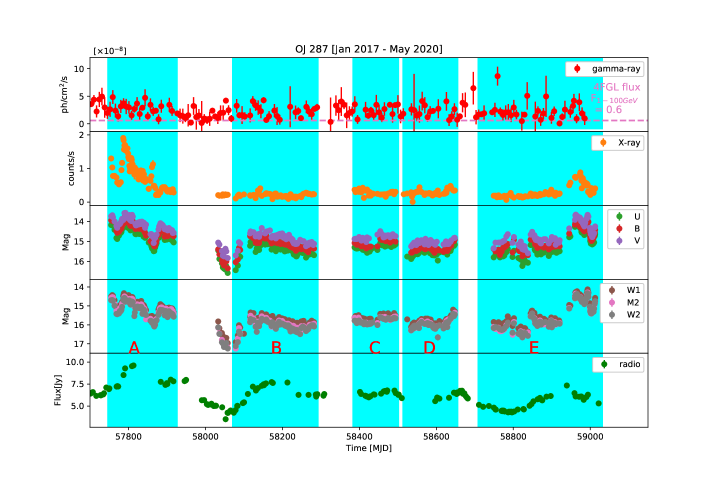
Figure 1: The upper plot shows the weekly binned gamma-ray light curve for 0.1–300 GeV. Panels 2nd, 3rd, and 4th are the Swift-XRT and UVOT light curves. The 5th panel is the radio light curve from OVRO at 15 GHz. The entire light curve is divided in five different states based on the flux and magnitude seen in Swift-XRT and UVOT. The various states are denoted as A, B, C, D, and E and their time duration is represented by the color patches.

2.2 X-ray Observations

On February 3, 2017, an X-ray flare was observed by the Swift-telescope, and the results were reported in Atel 10043. It is reported as the brightest flare ever detected since the monitoring started by the Swift-telescope. After that, many multiple flares were observed in X-rays until May 2020, and this whole period has been studied in this paper. Swift is a space-based telescope with three instruments onboard, observing all kinds of Galactic and extragalactic sources in soft $\&$ hard X-rays, Optical, and UV simultaneously. The working energy range of Swift-XRT is 0.3-10.0 keV. The BL Lac OJ 287 was observed by Swift-XRT telescope during the multiple flaring episodes in X-ray frequencies between the period January 2017 to May 2020. We have analyzed all the observations done during this period, and the processing of the raw data is done by using the task ‘xrtpipeline’ and cleaned events file are produced for each observation. The CALDB version 20160609 is used while processing the raw data. Our analysis is focused on only the Photon Counting mode observations, and the task ‘xselect’ is used for source and background selection. We have selected a region of 12 arc seconds around the source and away from the source for the source and background, respectively, in our data analysis. The task ‘xselect’ is also used to extract the spectrum and light curve, and the modeling of the spectrum is done in ‘Xspec’(Arnaud 1996). For modeling the spectra, we have used a single power-law model. The Galactic absorption column density $n_{H}$ = 1.10$\times$10²⁰ cm^-2 is fixed from Kalberla et al. (2005). The modeling is done for an energy range of 0.3 – 10.0 keV.

2.3 Optical and UV Observations

Having the Swift Ultraviolet/Optical Telescope (UVOT, Roming et al. 2005) on board with Swift-XRT has the advantage of getting simultaneous observations in Optical and UV bands. Swift-UVOT has also observed the OJ 287 in all of the available six filters U, V, B, W1, M2, and W2, simultaneously with the X-ray observations. The source instrumental magnitudes are extracted following the $uvotsource$ procedure. We have considered the region of 5 arcsec around the source and away from it as the source and the background region, respectively, in our data analysis. The magnitudes are corrected for galactic extinction by using the reddening E(B-V) = 0.0241 from Schlafly & Finkbeiner (2011) and zero points from Breeveld et al. (2011). Moreover, the magnitudes are converted into flux by multiplying by the conversion factor estimated by Poole et al. (2008) and the ratios of extinction to reddening from Giommi et al. (2006).

In the period between Feb 2019 - Jan 2020, we performed observations of OJ 287 using five different telescopes around the globe, which are: 2.15 m Jorge Sahade telescope (JS, telescope A) and 60  cm Helen Sawyer Hogg telescope (HSH, telescope B), CASLEO, Argentina; 1.3 m JC Bhattacharya telescope (JCBT; telescope C) at the Vainu Bappu Observatory (VBO), India. The technical descriptions of the above telescopes are summarized in Table 1 of Agarwal et al. (2019) and Agarwal et al. (2021). The number of observations made in each band on a particular date during our monitoring campaign is provided in Table 1.

The preliminary data reduction includes bias correction, flat fielding, and cosmic-ray removal, which was performed with IRAF software. We then processed the cleaned CCD images using the Dominion Astronomical Observatory Photometry (DAOPHOT II) software (Stetson, 1987, 1992) using the aperture photometry technique through which we obtained instrumental magnitudes for our target and four standard stars located in the same field. A more detailed and comprehensive description of data reduction methods used is given in Section 2 of Agarwal et al. (2019). Finally, to extract the instrumental differential light curves (LCs), we selected two non-variable standards having magnitude and color very similar to that of the blazar. The calibrated LCs were obtained using the star 10 of Fiorucci & Tosti (1996). After constructing the calibrated LCs of our source, we carefully inspected the LCs for any outliers. A handful of such suspicious data points were detected and corrected.

2.4 Radio data at 15 GHz

Owens Valley Radio Observatory(OVRO; Richards et al. 2011) is one of the observatories that monitors the bright Fermi detected blazars. It is a 40-meter single-dish antenna working at a frequency of 15 GHz. A large number of Fermi blazars are continuously monitored by OVRO twice a week. Our candidate source, OJ 287, is also part of the OVRO monitoring program, and we have collected the data from September 2017 to July 2020.

Table 1: Log of photometric observations for the blazar OJ 287.

Date of	Telescope	Number of data points
observations
(yyyy mm dd)		$B$	$V$	$R$	$I$
2019 02 15	C	0	1	6	1
2019 02 27	A	3	2	30	2
2019 03 01	A	2	9	27	1
2019 03 02	A	0	9	22	1
2019 03 03	A	1	17	16	2
2019 03 09	C	1	1	1	1
2019 03 11	C	1	1	1	1
2019 03 12	C	0	1	1	0
2019 03 13	C	1	1	1	1
2019 03 26	A	2	1	24	2
2019 04 05	C	1	1	17	1
2019 04 06	C	1	1	10	1
2019 04 07	C	1	2	20	2
2019 04 09	A	1	16	16	1
2019 04 10	A	2	10	10	2
2019 04 10	A	3	4	12	2
2019 04 11	A	2	12	14	2
2019 12 17	A	0	1	9	2
2020 01 03	A	2	2	120	2
2020 01 27	B	0	4	4	1

Table 2: Table shows the fractional variability and the variability time estimated for various states in different waveband as shown in Figure 1, and explained in section 3.1.1 in detail.

Instrument	Various states	Fractional variability	Variability time
		Fvar	$\tau_{var}$[days]
XRT	A	0.48$\pm$0.01	2.41
XRT	B	0.29$\pm$0.01	2.39
XRT	C	0.25$\pm$0.01	2.32
XRT	D	0.28$\pm$0.01	0.80
XRT	E	0.57$\pm$0.01	0.98
UVOT-U	A	0.284$\pm$0.003	4.99
U	B	0.215$\pm$0.004	3.19
U	C	0.103$\pm$0.006	15.83
U	D	0.164$\pm$0.005	6.94
U	E	0.585$\pm$0.003	0.58
UVOT-B	A	0.191$\pm$0.032	3.75
B	B	0.221$\pm$0.004	3.18
B	C	0.140$\pm$0.006	19.70
B	D	0.152$\pm$0.005	3.56
B	E	0.483$\pm$0.003	1.26
UVOT-V	A	0.272$\pm$0.003	5.25
V	B	0.228$\pm$0.005	4.04
V	C	0.104$\pm$0.008	10.33
V	D	0.088$\pm$0.007	2.82
V	E	0.499$\pm$0.004	0.76
UVOT-W1	A	0.303$\pm$0.003	5.44
W1	B	0.205$\pm$0.005	5.97
W1	C	0.096$\pm$0.007	11.26
W1	D	0.203$\pm$0.006	6.86
W1	E	0.599$\pm$0.004	0.95
UVOT-M2	A	0.305$\pm$0.001	4.00
M2	B	0.222$\pm$0.002	5.06
M2	C	0.117$\pm$0.003	19.67
M2	D	0.205$\pm$0.003	6.53
M2	E	0.635$\pm$0.002	3.80
UVOT-W2	A	0.308$\pm$0.003	4.15
W2	B	0.214$\pm$0.004	4.60
W2	C	0.111$\pm$0.006	19.28
W2	D	0.221$\pm$0.006	3.53
W2	E	0.628$\pm$0.004	1.08

Table 3: Results of INV observations of OJ 287.

Date of observation	Passband	$N$	$\sigma_{1}$	$\sigma_{2}$	$\Gamma_{\rm SF}$	$C$-test	$F$-test	Variable (?)
(yyyy mm dd)
(1)	(2)	(3)	(4)	(5)	(6)	(7)	(8)	(9)
27.02.2019	R	30	0.0063	0.0027	1.1219	2.3389	5.4705	PV
01.03.2019	R	27	0.0105	0.0041	1.1073	2.5505	6.5051	PV
02.03.2019	R	22	0.0031	0.0037	1.1287	0.8236	1.4741	NV
03.03.2019	R	16	0.0026	0.0033	1.1166	0.7715	1.6802	NV
	V	17	0.0143	0.0075	1.1177	1.8953	3.5921	NV
26.03.2019	R	24	0.0064	0.0027	1.0808	2.3377	5.4647	PV
05.04.2019	R	17	0.0117	0.0133	1.1345	0.8754	1.3049	NV
06.04.2019	R	17	0.0139	0.0128	1.1406	1.0883	1.1845	NV
07.04.2019	R	20	0.0289	0.0088	1.0617	3.2657	10.665	Var
09.04.2019	R	16	0.0119	0.0063	1.0389	1.8821	3.5423	NV
	V	16	0.0182	0.0068	1.0549	2.6690	7.1238	Var
10.04.2019	R	10	0.0052	0.0055	1.0721	0.9523	1.1027	NV
	V	10	0.0068	0.0024	1.0890	2.8971	8.3932	Var
10.04.2019	R	12	0.0058	0.0049	1.0980	1.1759	1.3828	NV
11.04.2019	R	14	0.0086	0.0042	1.0969	2.0671	4.2730	PV
	V	12	0.0140	0.0035	1.0994	3.9829	15.863	Var
03.01.2020	R	120	0.0076	0.0050	0.9357	1.5211	2.3137	PV

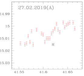
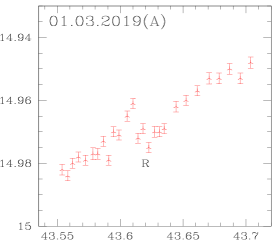
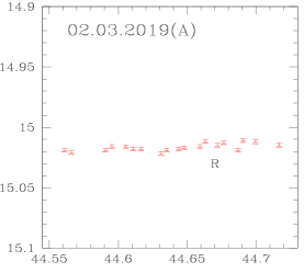
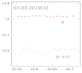
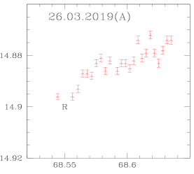
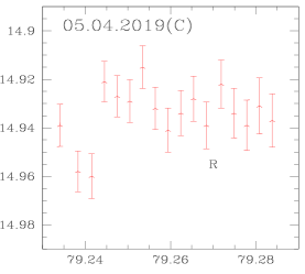
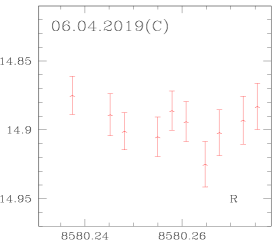
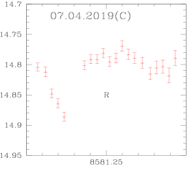
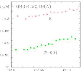
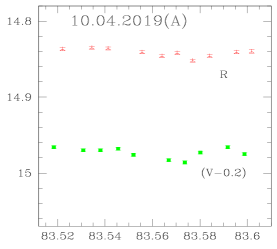
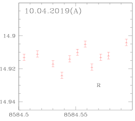
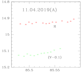
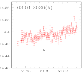
Figure 2: Light curves for OJ 287; green denotes $V$ band while red denotes $R$ filter. In each plot, X axis is JD and Y axis is the source magnitude. Observation date and the telescope used are indicated in each plot viz. Telescope A, is JS (2.15 m Jorge Sahade telescope), telescope B, HSH (Helen Sawyer Hogg telescope), and telescope C, JCBT (Vainu Bappu Observatory (VBO), India).

3 Results

A detailed temporal and spectral study has been done using the multi-wavelength data from the Fermi-LAT, Swift-XRT/UVOT telescope. The archival data from OVRO are used to perform the correlation study with the gamma-ray.

3.1 Multi-waveband Fractional and Temporal Variability

3.1.1 Multi-waveband Variability

OJ 287 is mentioned as a gamma-ray source in 3FGL (Acero et al. 2015) as well as in 4FGL (Abdollahi et al. 2020) catalog by Fermi-LAT. The blazar OJ 287 is one of the most active blazars with a binary black hole system, and that makes it one of a kind and thus an interesting source in the Fermi-LAT catalog. It is monitored by various ground-based and space-based telescopes across the entire wavelength range. The recent flare seen by Swift-XRT and UVOT during the beginning of the year 2020 has been confirmed as the second brightest flare in X-ray and optical/UV (Komossa et al., 2020b).

The multi-wavelength light curve, since January 2017 to May 2020, from radio (at 15 GHz) to gamma-ray (0.1–300 GeV) is shown in Figure 1. The whole light curve is divided into various activity states based on the variability and flux states seen in X-ray, optical, and UV. The states are defined as A, B, C, D, and E. Among all these five states, state A and E have higher mag/flux values in optical/X-ray and considered to be flaring states. The X-ray flare in state A was earlier studied by Kushwaha et al. (2018b), and Kapanadze et al. (2018). They found strong positive correlation between optical, UV and X-ray outbursts. Our results are consistent with them, which suggests that the same population of electrons is generating the optical, UV and X-ray outbursts. The flare in optical and X-ray band during the state E is widely reported in many astronomer’s telegram (Zola et al. 2020, Komossa et al. 2020a, Reinhart et al. 2020, Hosokawa et al. 2020, Komossa & Grupe 2020) and studied by Komossa et al. (2020b) and Kushwaha et al. (2020). Here, we provide a broadband temporal and spectral analysis of these states and the broadband SED modeling is also done to compare the jet parameters between various high (A & E) and low (B, C, & D) states.

The upper panel shows the gamma-ray light curve by Fermi-LAT. It is found that the source is not very bright in gamma-ray. The variation in flux is nearly a factor of $5$ between its lowest and highest flux state. The average flux during this period is 2.65$\times$10^-8 ph cm^-2 s^-1. The average flux from the 4FGL catalog for 1$-$100 GeV is 0.6$\times$10^-8 ph cm^-2 s^-1 shown by a horizontal dashed line in Figure 1. In the last segment of the light curve for the period 2017 - 2020, the gamma-ray data show their highest flux of around 1.0$\times$10^-7 ph cm^-2 s^-1.

The X-ray light curve is shown in the second panel. It is observed that the source is most variable during the first and fifth states, and the flux became maximum in early 2017. The highest flux state in X-ray coincides with the high flux state in radio and optical/UV. In gamma-ray, the flux is not much high, but the variability can be seen in the light curve.

The light curves for various bands of optical and UV are shown in panels 3rd and 4th. The source seems to be variable across the whole light curve and achieving its maxima in early 2017 and mid 2020. These light curves are similar to the X-ray light curve, which suggests the link between their production site and their physical processes. The multi-wavelength SED modeling is done later in this paper to discuss these possibilities.

The 5th panel shows the simultaneous observations in radio at 15 GHz. The light curve reveals that the source is variable in radio and the maximum variation is a strong decrease from 10 to 1 Jy.
The fractional variability estimated for various states is reported in Table 2. The fractional variability is used to characterize the long-term variability in various bands. It is formulated by Vaughan et al. (2003) as:

$$F_{\rm var}=\sqrt{\frac{S^{2}-err^{2}}{F^{2}}},$$ (1)

where, F denotes the mean flux, S² and err² are the variance and the mean square error in the flux, respectively. The error in flux variability amplitude is given in Prince (2019). The fractional variability amplitude estimated for the various states in all wavebands is depicted in Table 2.

The flux doubling/halving time is also estimated for all the states in all bands. The values are further used to characterize the variability in OJ 287. The flux doubling time is also known as variability time, is defined as (Zhang et al., 1999)

$$t_{d}=\frac{(F_{1}+F_{2})(T_{2}-T_{1})}{2|F_{2}-F_{1}|}$$ (2)

where, F₁, and F₂ are fluxes at time T₁ and T₂. The doubling time or the fastest (or shortest) variability time (t_var) considered as the smallest value among the available pairs in the light curve. The variability amplitude and the doubling time together characterize the variability of the source in various states. In segment E, the source appeared to be more variable with the highest variability amplitude among all the states in all wavebands and have the shortest (fastest) variability time of the order of 1 day (Table 2). The values of variability amplitude vary from 50$\%$ to 60$\%$ among all the wavebands and the shortest variability time of OJ 287 during 2017 to 2020 in X-ray is nearly 1 day.

The radio data are very sparse during this entire period, and hence we did not include them in the variability study to draw any meaningful conclusion.

3.1.2 Intra-day Variability (IDV)

Considering the modest number of observations in each passband, the variability of the source is measured using the C-criterion, which compares the dispersion in the (blazar-comparison star) and control star - comparison star. We also used the F test, which is the ratio of the variances of the blazar instrumental light curve (LC) to that of the standard star. The above tests are discussed in more detail in Agarwal et al. (2019). As claimed by Zibecchi et al. (2017), dispersion scaling by the Howell ($\Gamma_{\rm SF}$) factor (Howell et al., 1988) to match the control star and the target error distributions result in the most reliable results. We call a particular LC to be variable (Var) only when both tests reject the null hypothesis at 99.5% confidence level, possibly variable (PV) if just one of the tests rejects the null hypothesis, and non-variable (NV) if both tests fail to reject the null hypothesis. Intraday variability (IDV) results for our observation campaign are summarized in Table 3 where columns 1 – 8 are, respectively, observation date, the passband of observation, number of data points in the given passband, dispersion of blazar differential LC (DLC), dispersion of the control star DLC, Howell’s factor, results for $C$-test and $F$-test. The variability state of the source is given in column 9. Our total monitoring coverage contains 13 intraday LCs. The IDV behavior of OJ 287 over the entire duration is displayed in Figure 2. We found only 1 LC (i.e., April 07, 2019) to be variable according to our conditions, while 5 LCs were PV. On the remaining seven nights, the source was found to be NV. Our intraday LCs span a duration of 2 – 4 hours. Therefore, the relatively short span of observations reduces the chances of detecting genuine variability. The highest level recorded for OJ 287 was in 2015 Dec by Gupta et al. (2017). OJ 287 has been monitored for more than a century and has R band data available since 1890. It is one of the extensively studied sources using both photometry and polarimetry observations on diverse timescales. During the 2015 flare, the source attained a V mag of $\sim$13.4, R mag of $\sim$ 13.0 while I mag $\sim$ 12.4. From the current monitoring session, we found the brightest state reached by the source was on January 03, 2020, with R $\sim$ 14.38 mag, fainter than its brightest state in 2015 by $\sim$ 1.4 mag while the faintest state attained by the source was on December 18, 2019, with R band mag of 15.15, approximately 2.15 mag fainter than its brightest state during 2015 – 2016 outburst. Significant optical LTV is also observed for the source with an R band magnitude change of $\sim$ 2 (Fig. 1). The variability trends observed during our monitoring period are quite different from the previous ones (Gupta et al., 2017). The target did not display high IDV during the current phase, which could be due to the lesser data cadence.

3.2 Gamma-ray Spectral Analysis

We have also produced the gamma-ray spectra for all the various states of the source identified in Figure 1. The gamma-ray spectra are produced with the help of likeSED.py a python code provided by the Fermi Science Tools. First, the Likelihood analysis is done with the default spectral model power-law (PL) to model the spectral data points, and further, we have changed the model to various other models, like log parabola (LP) and broken power law (BPL) to get the best fit. The details about the models are discussed in Prince et al. (2018). The isotropic $\gamma$-ray luminosity corresponding to each spectral models are estimated during all the segments by following the equation 5 of Prince et al. (2021), and the values are of the order of 10⁴⁷ $-$ 10⁴⁸ erg/s, which are lower than the Eddington luminosity (10⁵⁰ erg/s) of this source as estimated in Section 3.4. The estimated $\gamma-ray$ luminosity values are mentioned in Table 4. The gamma-ray spectrum and model fitting are shown in Figure 3, and corresponding model parameters are presented in Table 4. Considering the PL spectral model, the spectral state of the source changes from segment A to Segment B, C, and D from harder ($\Gamma_{\rm PL}$ = 1.90$\pm$0.06) to softer ($\Gamma_{\rm PL}$ = 2.27$\pm$0.08)) and again it becomes harder from segment D ($\Gamma_{\rm PL}$ = 2.35$\pm$0.10) to segment E ($\Gamma_{\rm PL}$ = 2.21$\pm$0.06).

The Likelihood analysis returns the TS (test statistics; TS $\sim$ 25, which corresponds to 5$\sigma$ significance; Mattox et al. 1996) corresponding to each model and is generally used to decide which model gives the best to the spectral data points. So finally, we measure the TS_curve = 2(log L(LP/BPL) - log L(PL)), where L represents the likelihood function (Nolan et al., 2012). The TS_curve reveals the presence of curvature or a break in the spectrum, and which could be caused by the absorption of high energy photons ($>$ 20 GeV; Liu & Bai 2006) by the broad-line region (BLR), assuming the emitting region is located within the BLR. However, if the emitting region is located outside the BLR, a nice power-law spectral behavior is expected. The best spectral model favors the large positive value of TS_curve over the low value of TS_curve.

The various models and their corresponding parameters are exhibited in Table 4. The values of TS_curve are close to each other for the different models. TS values are nearly equal for the PL and LP models but differ with BPL. However, there is no clear trend in the spectral model that can explain the $\gamma$-ray sed from all the segments, which shows that the source has a very complex behavior during 2017$-$2020.

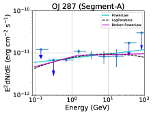
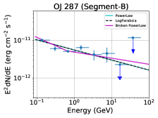
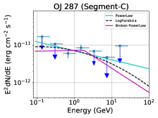
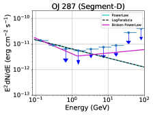
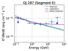
Figure 3: Gamma-ray SED of all the segments identified during 2017$-$2020 in OJ 287 are modeled with three different spectral models PL, LP, and BPL (see Section 3.2 for more details). The down arrow represents the upper limit in that particular segment.

Table 4: The modeled parameters of gamma-ray SED for all the segments identified in Figure 1. Column 3 shows the isotropic $\gamma$-ray luminosity during the various segments, which is lower than the Eddington luminosity ($\sim$10⁵⁰ erg/s) of the source as discussed in Section 3.4.

Various	F0.1-300GeV	Luminosity	PowerLaw			TS	TScurve
states	(10-8 ph cm-2 s-1)	(1048 erg s-1)	$\Gamma_{\rm PL}$
A	4.10$\pm$0.50	0.25	-1.90$\pm$0.06	–	–	570.20	–
B	4.90$\pm$0.60	0.80	-2.27$\pm$0.08	–	–	313.00	–
C	5.10$\pm$0.81	0.93	-2.24$\pm$0.10	–	–	173.22	–
D	5.40$\pm$0.81	1.04	-2.35$\pm$0.10	–	–	178.32	–
E	5.20$\pm$0.55	2.92	-2.21$\pm$0.06	–	–	551.28	–
			LogParabola
			$\alpha$	$\beta$
A	3.60$\pm$0.70	0.22	1.81$\pm$0.12	0.03$\pm$0.03	–	569.48	-0.72
B	4.90$\pm$0.60	0.81	2.27$\pm$0.08	0.00$\pm$0.00	–	313.01	0.01
C	4.70$\pm$0.96	0.84	2.19$\pm$0.13	0.05$\pm$0.07	–	173.64	0.42
D	5.40$\pm$0.81	0.96	2.35$\pm$0.10	0.00$\pm$0.00	–	178.30	0.02
E	5.20$\pm$0.55	2.45	2.21$\pm$0.06	0.00$\pm$0.00	–	551.24	-0.08
			Broken PowerLaw		Ebreak
			$\Gamma_{1}$	$\Gamma_{2}$	[GeV]
A	3.70$\pm$0.70	0.21	-1.77$\pm$0.17	-1.98$\pm$0.11	1.43$\pm$0.74	569.44	-0.76
B	5.30$\pm$0.30	1.03	-2.44$\pm$0.83	-2.16$\pm$0.09	0.64$\pm$0.25	315.26	2.26
C	3.60$\pm$1.20	1.08	-1.97$\pm$0.24	-2.64$\pm$0.36	1.78$\pm$0.16	144.38	-28.84
D	6.20$\pm$0.87	1.16	-2.64$\pm$0.14	-1.86$\pm$0.16	1.41$\pm$0.13	186.32	8.00
E	5.80$\pm$2.00	3.02	-2.40$\pm$0.45	-2.04$\pm$0.06	1.00$\pm$0.32	560.03	8.75

3.3 Correlations Studies

We have collected multi-wavelength data from 2017 to May 2020. Five different states are identified based on the flux and variability seen in X-rays and Optical/UV. During this period between January 2017 to May 2020, we have not observed any flare in gamma-ray, but the source is variable in this low state, as can be seen in the top panel of Figure 1. The source is flaring in X-ray and optical/UV and appears to be more variable in X-rays, optical, UV, and radio (15 GHz) wavebands, as shown in Figure 1 from top to bottom. Here we try to investigate the correlation between the X-ray and optical/UV emission for all the states since they have good coverage in all the wavebands. The observed time lags between light curves at different wavebands can be really helpful to locate their emission regions along the jet axis.

To estimate the correlation, we have followed the method developed by Edelson & Krolik (1988). Different bin sizes have been chosen in different combinations to examine the discrete correlation function (DCF) peaks. The DCF estimated for all the possible combinations between X-rays and UV/Optical are shown in Figure 4. The top row of the figure shows the DCF for state A and then followed by B, C, D, and E towards the bottom row. The correlation coefficients, time lags, and the bin size for all the combinations are mentioned in Table 5. Our results show that optical-X-ray and the UV-X-ray emissions for the states A, B, D, and E are highly correlated with values of correlation coefficient above 50$\%$ and with time lags within the bin size. This strong correlation with zero time lag suggests that these two emissions have a common emission region. However, for state C, we do not observe any correlation between Optical/UV and X-rays. We have also estimated the significance of the DCF peaks by simulating the 1000 artificial optical and UV light curves by following the monte carlo procedure described in Emmanoulopoulos et al. (2013), for PSD slope 1.5. The simulated light curves are cross-correlated with the observed X-ray light curves. Further, 2$\sigma$ and 3$\sigma$ significance is estimated, which are shown in red and blue dashed line in Figure 4. Our results show that in most of the cases, emissions are correlated above 2 $\sigma$ significance.

As can be seen in Figure 1, the radio data are very sparse, and hence we did not include it in the correlation study.

Table 5: DCF parameters for all the combinations. Most of the time lags were found within the binsize.

States	Combinations	DCF	Time lags	binsize
A	V vs X-rays	0.73$\pm$0.05	-2.06	10.0
	B vs X-rays	0.73$\pm$0.05	-2.06	10.0
	U vs X-rays	0.72$\pm$0.05	-2.06	10.0
	W1 vs X-rays	0.76$\pm$0.05	-2.06	10.0
	M2 vs X-rays	0.71$\pm$0.05	-2.06	10.0
	W2 vs X-rays	0.74$\pm$0.05	-2.06	10.0
B	V vs X-rays	0.37$\pm$0.09	-15.42	15.0
	B vs X-rays	0.43$\pm$0.08	-10.00	20.0
	U vs X-rays	0.37$\pm$0.09	-15.42	15.0
	W1 vs X-rays	0.44$\pm$0.12	-5.00	10.0
	M2 vs X-rays	0.43$\pm$0.10	-11.75	12.0
	W2 vs X-rays	0.46$\pm$0.10	-11.75	12.0
C	V vs X-rays	0.60$\pm$0.25	37.60	8.0
	B vs X-rays	0.41$\pm$0.22	40.00	10.0
	U vs X-rays	0.42$\pm$0.20	40.00	10.0
	W1 vs X-rays	0.38$\pm$0.28	46.00	8.0
	M2 vs X-rays	0.49$\pm$0.25	46.00	8.0
	W2 vs X-rays	0.35$\pm$0.11	29.27	8.0
D	V vs X-rays	0.50$\pm$0.13	-5.00	10.0
	B vs X-rays	0.57$\pm$0.13	-5.00	10.0
	U vs X-rays	0.61$\pm$0.12	-6.28	12.0
	W1 vs X-rays	0.66$\pm$0.14	-5.00	10.0
	M2 vs X-rays	0.63$\pm$0.13	-5.00	10.0
	W2 vs X-rays	0.63$\pm$0.12	-5.00	10.0
E	V vs X-rays	0.79$\pm$0.04	-5.00	10.0
	B vs X-rays	0.78$\pm$0.04	-5.00	10.0
	U vs X-rays	0.78$\pm$0.04	-5.00	10.0
	W1 vs X-rays	0.79$\pm$0.04	-5.00	10.0
	M2 vs X-rays	0.80$\pm$0.04	-5.00	10.0
	W2 vs X-rays	0.79$\pm$0.04	-5.00	10.0

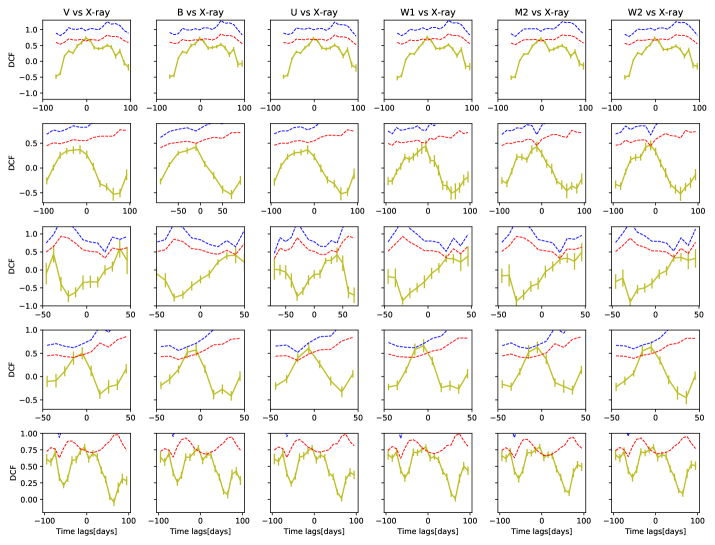
Figure 4: Cross-correlation of optical/UV vs X-ray. The five rows of the plot are the five states (A, B, C, D, E) defined in Figure 1. Horizontal red and blue dashed lines are 2$\sigma$ and 3$\sigma$ significance respectively. We do not observe any significant time lag in any of the combinations. During state C, we see some time lags but the correlation coefficient are below 50$\%$ and below 2$\sigma$ significance, and hence do not consider as an actual time lag.

3.4 Modeling the Multi-wavelength SEDs

Good coverage of OJ 287 in various wavebands provides an opportunity to obtain the multi-wavelength spectral energy distribution (MWSED), which has been used in our modeling. We have produced the MWSED using Swift-XRT, UVOT and Fermi-LAT data for all the observations in different states. The modeling of OJ 287 has been done previously in various ways. We assume that the emission region is in the jet of the primary black hole. The emission region is a spherical blob that is moving with Doppler factor $\delta$ down the jet. The shock accelerated leptons are losing energy inside this blob by synchrotron, and synchrotron self Compton (SSC) processes.

We have used a publicly available time-dependent code, GAMERA (Hahn 2015) to model the broadband SED. It is a python based code and needs an initial injected electron spectrum as an input which further solves the transport equation (3) and estimates the propagated electron spectrum. Finally, the propagated electron spectrum is used to calculate the emission from the various processes like Synchrotron, SSC, and EC by external photons of various origin (BLR, DT, accretion disk). We use the following transport equation to find the electron spectrum after energy loss:

$$\frac{\partial N(E,t)}{\partial t}=Q(E,t)-\frac{\partial}{\partial E}\Big{(}b(E,t)N(E,t)\Big{)}$$ (3)

where, $Q(E,t)$ is the input spectrum and $N(E,t)$ is the propagated one at a time ‘t’. $b(E,t)$ corresponds to the radiative loss by different physical processes, synchrotron, SSC, and EC scattering. We have assumed a LogParabola electron distribution as the injected electron spectrum in our modeling.

The MWSED could be modelled with the leptonic scenario where SSC (synchrotron self Compton) and EC (external Compton) emission are generating the high energy peak. The study by Kushwaha et al. 2013 on the 2009 flare suggests that the X-ray and $\gamma$-ray emission can be explained by SSC and EC processes respectively, where the seed photons for the external Compton are originated by a thermal bath of 250 K located at distance of $\sim$9 pc from the SMBH. In a more recent study by Kushwaha et al. 2018a the December 2015 - May 2016 high state has been modelled using both SSC and EC emissions. The December 2015 high activity has been predicted to occur from the impact of the second black hole on the accretion disk of the primary black hole. The non thermal emission showed nearly co-spatial origin. They modelled the gamma ray flux by external Compton emission of relativistic electrons by optical-UV line emission, which shows the signature of a blue bump in the optical-UV flux. They fitted the X-ray data with SSC emission. In the present study we find that the source is variable in all wavebands including $\gamma$-ray, though we did not see any flaring behavior in this band. The observed day scale variability time in gamma-ray flux suggests the location of the emission region close to the SMBH, within a few parsec from the base of the jet. The variability study across all the wavebands exhibits an order of day scale flux variability, due to this reason we model the broadband SED with only synchrotron and SSC within a single emission zone. The correlation study also suggests that the emissions are produced at the same location.

The SSC emission is determined by the synchrotron emission and the size of the emission region. The synchrotron emission depends on the magnetic field in the emission region in the jet and the energy of the leptons. The size of the emission region can be constrained by the variability time scale. Considering 1 day variability time in the gamma-ray data, we have estimated the size of the emission region by the following relation r$\sim$ c t_var $\delta$/(1+z), where $\delta$ = 20, and it is found to be r$\sim$4.0$\times$10¹⁶cm.

However, in our modeling the size of the emission region is a free parameter and we have found that a smaller size of the emission region is required to explain the broadband SED.

We also have many other parameters in our model, e.g., magnetic field, injected electron spectrum, lower and higher energy cut-offs in the injected electron spectrum, normalization of the electron spectrum, and these are optimized to achieve the best SED fit. The MWSED modeling results are depicted in Figure 5 for the various states, and their corresponding best-fit parameters are tabulated in Table 6. States C $\&$ D are very similar to each other in variability and flux states, and hence we only show the SED modeling of state C. The modeling confirms that the low and high energy peaks can be constrained with synchrotron and SSC, respectively. In Figure 5, it has been noticed that the source has more emission in Optical-UV than in $\gamma$-ray. Hence a large value of magnetic field ($\sim$4-7 Gauss) is used to fit the data.

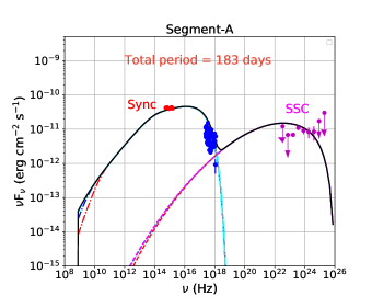
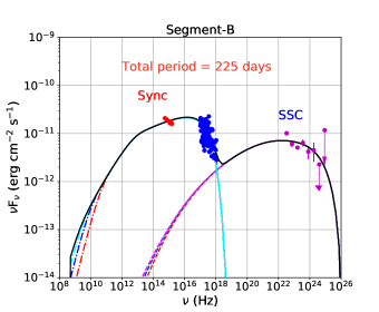
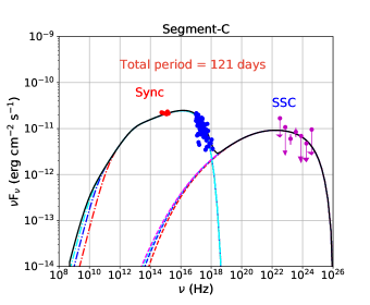
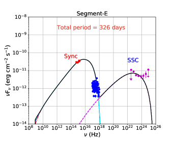
Figure 5: The MWSED for all the various segments observed during the year 2017$-$2020. The ‘dotted dahsed’ and ‘dahsed’ line in different colors in Synchrotron and SSC peaks are the time evolution of the model. The down arrow represents the $\gamma$-ray upper limits. The optical/UV, X-ray, and $\gamma$-ray data points are shown in red, blue, and magenta colors respectively.

The previous broadband SED modeling of OJ 287 at different occasions of low and bright state (Kushwaha et al. 2013, Kushwaha et al. 2018a, b) was carried out with a range of values of the Doppler and Lorentz factor. In this study, we have fixed the Doppler and Lorentz factor of the blob at 20 and 15.5 respectively, which are similar to the values reported in earlier papers.

Table 6: Multi-wavelength SED modeling results with the best fitted parameters values. The input injected electron distribution is LogParabola with reference energy 60 MeV. The Doppler factor and the Lorentz factor are fixed at 20.0 and 15.5 respectively.

high state	Parameters	Symbols	Values	Period
Segment-A				183 days
	Size of the emitting zone	r	2.6$\times$1015 cm
	Min Lorentz factor of emitting electrons	$\gamma_{min}$	350.0
	Max Lorentz factor of emitting electrons	$\gamma_{max}$	2.8$\times$104
	Input injected electron spectrum (LP)	$\alpha$	1.60
	Curvature parameter of the PL spectrum	$\beta$	0.02
	Magnetic field in emitting zone	B	5.9 G
	Jet power in electrons	Pj,e	4.35$\times$1044 erg/s
	Jet power in magnetic field	Pj,B	2.12$\times$1044 erg/s
	Jet power in protons	Pj,P	3.39$\times$1043 erg/s
	Total jet power	Pjet	6.81$\times$1044 erg/s
Segment-B				225 days
	Size of the emitting zone	r	2.6$\times$1015 cm
	Min Lorentz factor of emitting electrons	$\gamma_{min}$	120.0
	Max Lorentz factor of emitting electrons	$\gamma_{max}$	3.6$\times$104
	Input injected electron spectrum (LP)	$\alpha$	1.68
	Curvature parameter of the PL spectrum	$\beta$	0.005
	Magnetic field in emitting zone	B	4.2 G
	Jet power in electrons	Pj,e	2.59$\times$1044 erg/s
	Jet power in magnetic field	Pj,B	1.07$\times$1044 erg/s
	Jet power in protons	Pj,P	3.56$\times$1043 erg/s
	Total jet power	Pjet	4.02$\times$1044 erg/s
Segment-C				121 days
	Size of the emitting zone	r	2.6$\times$1015 cm
	Min Lorentz factor of emitting electrons	$\gamma_{min}$	160.0
	Max Lorentz factor of emitting electrons	$\gamma_{max}$	3.6$\times$104
	Input injected electron spectrum (LP)	$\alpha$	1.68
	Curvature parameter of the PL spectrum	$\beta$	0.005
	Magnetic field in emitting zone	B	4.2 G
	Jet power in electrons	Pj,e	2.96$\times$1044 erg/s
	Jet power in magnetic field	Pj,B	1.07$\times$1044 erg/s
	Jet power in protons	Pj,P	4.06$\times$1043 erg/s
	Total jet power	Pjet	4.44$\times$1044 erg/s
Segment-E				326 days
	Size of the emitting zone	r	2.6$\times$1015 cm
	Min Lorentz factor of emitting electrons	$\gamma_{min}$	1.4$\times$103
	Max Lorentz factor of emitting electrons	$\gamma_{max}$	1.5$\times$104
	Input injected electron spectrum (LP)	$\alpha$	1.6
	Curvature parameter of the PL spectrum	$\beta$	0.005
	Magnetic field in emitting zone	B	6.7 G
	Jet power in electrons	Pj,e	3.26$\times$1044 erg/s
	Jet power in magnetic field	Pj,B	2.73$\times$1044 erg/s
	Jet power in protons	Pj,P	1.32$\times$1043 erg/s
	Total jet power	Pjet	6.12$\times$1044 erg/s

We have also estimated the total jet power and the power in the individual component of the jet. The components are leptons, magnetic fields, and protons. We assume that the number ratio of leptons to protons is 20:1 in the jet and estimate the jet power in leptons and protons separately. The total jet power is generally defined as,

$$P_{jet}=\pi r^{2}\Gamma^{2}c(U^{\prime}_{e}+U^{\prime}_{B}+U^{\prime}_{p})$$ (4)

where, $U^{\prime}_{e}$, $U^{\prime}_{B}$, and $U^{\prime}_{p}$ are the energy densities in leptons, magnetic field and protons in the jet or co-moving frame. The values of the size of the emission region (‘$r$’) and the Lorentz factor ($\Gamma$) are already provided in the discussion above.

The total jet power calculated for all the states is shown in Table 6, and the value is much smaller than the Eddington luminosity of the source. The Eddington luminosity for the primary BH is estimated as L_Edd = 4$\pi$Gmm_pc/$\sigma_{T}$, where ‘m’ is the mass of the primary BH, m_p is the proton mass, and $\sigma_{T}$ is the Thompson scattering cross-section. The primary BH mass is estimated by Kushwaha et al. (2018a) by modeling the NIR-optical spectrum with an accretion disk, and the reported value is $\sim$1.8$\times$10¹⁰M_⊙. The Eddington luminosity is estimated to be 2.30$\times$10⁵⁰ erg/s, which is much higher than the total jet power estimated in this study by SED modeling. Modeling the high optical flux state with synchrotron emission requires a higher value of the magnetic field and hence higher jet power in the magnetic field. It is found that during the flaring state A & E the total jet power is 1.5 times higher than the total jet power estimated for low state B & C. The SED modeling also suggests that more luminosity in high energetic electrons is required to produce the broadband emission during flaring states A & E. The non thermal flares during state A and state E might have resulted from disk impact in November-Dec 2015 (Valtonen et al. 2016) and July-September 2019 (Laine et al. 2020) respectively when thermal flares were observed. The injection of high energetic electrons in jet could be due to the time delayed increase in the accretion rate and jet activity triggered by disk impact of secondary black hole or by tidal disruption events Sundelius et al. (1997). The variable accretion rate causes internal shock in the jet which accelerates electrons and they lose energy radiatively (Valtonen et al. 2006). The model of Sundelius et al. (1997) predicted a major increase in accretion rate in beginning of January 2020. However, the non-thermal flares happened during April-June 2020 nearly 4 months after their predicted time. The physical explanation for this delay requires a better understanding of the disk-jet connection as discussed by Komossa et al. (2020b).

4 Discussions and Conclusions

During the period between 2017 – 2020, the blazar OJ 287 did not show any bright flaring states in $\gamma$-ray. However, high flux states were reported across the optical-UV and X-ray wavebands in various Atels notifications, during that period. Also, variability in flux was observed in optical, UV, X-ray and gamma-ray frequency. Five states have been identified as A, B, C, D, & E based on the flux and fractional variability seen in optical-UV and X-rays. States A and E appear to be the brightest among all others in Figure 1, which can also be verified by the total jet power (Table 6) found from the modeling of these states. The variability time found across the bands ranges from 12 hr to    20 days across all states. The fastest variability time in X-rays is found to be of the order of 1 day. The optical bands U, B, & V have the shortest variability time of $\sim$ 14 hr, 30 hr, & 18 hr, while in UV bands, they are of the order of 1 day, 4 days, and 1 day for W1, M2, & W2 bands respectively. Though the source was not bright in $\gamma$-rays, we have produced the $\gamma$-ray spectrum for the different states to see if there is any variation in the spectrum. The gamma-ray data shows day scale variability and the maximum variation in flux between high and low state is found to be 5 times. The $\gamma$-ray data can be well fitted with PL or LP model. The values of the test statistics are similar for both the models. Further, we have estimated the correlations between various wavebands in order to understand whether they have a common emission region. The results show that emission is highly correlated (within the errorbars) between the different bands, which suggests their co-spatial origin. A single-zone emission model is applied to explain the multi-wavelength emission by performing the MWSED modeling. The SED modeling confirms the presence of high magnetic field in the jet and that the jet emission is powered by relativistic electrons.

In the binary black hole model the primary black hole is surrounded by an accretion disk. The orbit of the secondary black hole around the primary black hole is such that it intersects the accretion disk of the primary black hole two times. The major outbursts which occur at approximately 12 years of interval could be due to tidally induced mass flows. One such outburst is expected for every pericenter passage of the secondary (Sundelius et al. 1997). Pihajoki et al. (2013) theoretically predicted the timings of the precursor flares and compared with the observed flares in the light curve of OJ 287. Based on the model of Sundelius et al. (1997) a major after-flare is expected in January 2020, but it was observed in May 2020. The various physical conditions which affect this time delay are disk/corona properties and geometry, magnetic field geometry, shock formation in the jet. They are not yet well understood (Komossa et al. 2020b), which makes it very hard to predict this time delay from first principle.

The disk impact model predicts thermal bremmsstrahlung radiation as outbursts in optical-UV frequency due to the impact of the secondary black hole on the accretion disk of the primary black hole Lehto & Valtonen (1996). This model successfully predicted the impact flares in 2007, 2015, 2019 (Dey et al. 2021). The disk impact triggers time delayed increase in accretion rate and jet activity which leads to after-flare effects. The flares in state A & E in our work can be explained with this model. During states B, C, D there was no flare, hence a lower jet power is needed to model these low states.

Microvariability studies of blazars are one of the most relevant probes to understand the physical conditions very close to the central supermassive black hole. The exact phenomenon behind IDV in blazars is still under debate. Flux variations in blazars on intraday timescales almost certainly arise from intrinsic factors that are inherent to the blazar jets such as shocks in the helical jets (Calafut & Wiita, 2015) or blobs of plasma traversing through the Doppler boosted magnetized jet or formation of ultra-relativistic mini jets in the helical jet itself. In the low state of blazars, an alternative source for optical IDV is the accretion disc (AD, e.g. Chakrabarti & Wiita, 1993). According to the AD-based models, instabilities or hot spots or any other enhanced emission on the AD can yield optical IDV in blazars when the source is in a low state. The presence of confirmed IDV on only 1 night out of 13 nights could be most likely due to a uniform jet emission and any change in the direction of the relativistic shock with respect to our line of sight (LOS) if at all present, is very weak. LTV in blazars can be attributed to both intrinsic and extrinsic factors. Extrinsic mechanisms involve geometrical effects such as deviation of the emitting region with respect to LOS, thus causing variation in the Doppler factor (Villata et al., 2009) which in turn is observed as a variation on a long-term basis. Long-term flux variations in blazar LCs can also be caused by the launching of the new shocks. In general, optical IDV in blazars involve both intrinsic and extrinsic mechanisms (Pollack et al., 2016) and are usually difficult to disentangle.

Komossa et al. (2020b) studied the large X-ray data sample from 2015 to 2020, and their results pose a few fundamental questions. They observed the strong flare in X-ray, optical, and UV bands. The observation at the peak of the X-ray flare shows a steep power-law spectrum with index 2.8, which is very rare in blazars but consistent with the synchrotron origin of X-ray emission. They concluded that the emission is jet-driven and which is consistent with the binary black hole model. In another study by Kushwaha et al. (2020), the spectral change in X-ray emission was noted during 2017 to 2020, and they also suggested that it could be an emission from the jet. Here we have modeled the various low and high states observed during 2017 to 2020 considering the emissions are produced inside the jet.

It was reported earlier by Kushwaha et al. (2018a) that the source was active during December 2015 $-$ April 2016 in IR to $\gamma$-ray frequency. However, another study by Kushwaha et al. (2018b) for the period of June 2016 $-$ September 2017 found that the source was very bright in IR to X-ray, but no variability was seen in $\gamma$-ray. A similar kind of behavior is seen during early 2017 and mid 2020 when the source is flaring in optical-UV and X-ray but not very active in $\gamma$-ray. The different behaviors at different frequencies and at different epochs of time make this source very complex in nature. Many more observational and theoretical studies are required to understand the complex nature of the blazar OJ 287.

References

- Abdollahi et al. (2020) Abdollahi, S., Acero, F., Ackermann, M., et al. 2020, ApJS, 247, 33
- Acero et al. (2015) Acero, F., Ackermann, M., Ajello, M., et al. 2015, ApJS, 218, 23
- Agarwal et al. (2019) Agarwal, A., Cellone, S. A., Andruchow, I., et al. 2019, MNRAS, 488, 4093
- Agarwal et al. (2021) Agarwal, A., Mihov, B., Andruchow, I., et al. 2021, A&A, 645, A137
- Agarwal et al. (2017) Agarwal, A., Mohan, P., Gupta, A. C., et al. 2017, MNRAS, 469, 813
- Andrew et al. (1971) Andrew, B. H., Harvey, G. A., & Medd, W. J. 1971, Astrophys. Lett., 9, 151
- Andruchow et al. (2011) Andruchow, I., Combi, J. A., Muñoz-Arjonilla, A. J., et al. 2011, A&A, 531, A38
- Arnaud (1996) Arnaud, K. A. 1996, in Astronomical Society of the Pacific Conference Series, Vol. 101, Astronomical Data Analysis Software and Systems V, ed. G. H. Jacoby & J. Barnes, 17
- Atwood et al. (2009) Atwood, W. B., Abdo, A. A., Ackermann, M., et al. 2009, ApJ, 697, 1071
- Breeveld et al. (2011) Breeveld, A. A., Landsman, W., Holland, S. T., et al. 2011, in American Institute of Physics Conference Series, Vol. 1358, American Institute of Physics Conference Series, ed. J. E. McEnery, J. L. Racusin, & N. Gehrels, 373–376
- Calafut & Wiita (2015) Calafut, V. & Wiita, P. J. 2015, Journal of Astrophysics and Astronomy, 36, 255
- Chakrabarti & Wiita (1993) Chakrabarti, S. K. & Wiita, P. J. 1993, A&A, 271, 216
- Dey et al. (2019) Dey, L., Gopakumar, A., Valtonen, M., et al. 2019, Universe, 5, 108
- Dey et al. (2021) Dey, L., Valtonen, M. J., Gopakumar, A., et al. 2021, MNRAS, 503, 4400
- Dey et al. (2018) Dey, L., Valtonen, M. J., Gopakumar, A., et al. 2018, ApJ, 866, 11
- Dickel et al. (1967) Dickel, J. R., Yang, K. S., McVittie, G. C., & Swenson, G. W., J. 1967, AJ, 72, 757
- Edelson & Krolik (1988) Edelson, R. A. & Krolik, J. H. 1988, ApJ, 333, 646
- Emmanoulopoulos et al. (2013) Emmanoulopoulos, D., McHardy, I. M., & Papadakis, I. E. 2013, Monthly Notices of the Royal Astronomical Society, 433, 907
- Fiorucci & Tosti (1996) Fiorucci, M. & Tosti, G. 1996, A&AS, 116, 403
- Giommi et al. (2006) Giommi, P., Blustin, A. J., Capalbi, M., et al. 2006, A&A, 456, 911
- Gupta et al. (2016) Gupta, A. C., Agarwal, A., Mishra, A., et al. 2016, Monthly Notices of the Royal Astronomical Society, 465, 4423
- Gupta et al. (2017) Gupta, A. C., Agarwal, A., Mishra, A., et al. 2017, MNRAS, 465, 4423
- Hahn (2015) Hahn, J. 2015, in International Cosmic Ray Conference, Vol. 34, 34th International Cosmic Ray Conference (ICRC2015), 917
- Hosokawa et al. (2020) Hosokawa, R., Adachi, R., Murata, K. L., et al. 2020, The Astronomer’s Telegram, 13755, 1
- Howell et al. (1988) Howell, S. B., Mitchell, K. J., & Warnock, A., I. 1988, AJ, 95, 247
- Kalberla et al. (2005) Kalberla, P. M. W., Burton, W. B., Hartmann, D., et al. 2005, A&A, 440, 775
- Kapanadze et al. (2018) Kapanadze, B., Vercellone, S., Romano, P., et al. 2018, MNRAS, 480, 407
- Kidger et al. (1992) Kidger, M., Takalo, L., & Sillanpaa, A. 1992, A&A, 264, 32
- Kinman (1975) Kinman, T. D. 1975, in IAU Symposium, Vol. 67, Variable Stars and Stellar Evolution, ed. V. E. Sherwood & L. Plaut, 573
- Komossa & Grupe (2020) Komossa, S. & Grupe, D. 2020, The Astronomer’s Telegram, 13785, 1
- Komossa et al. (2020a) Komossa, S., Grupe, D., & Gomez, J. L. 2020a, The Astronomer’s Telegram, 13658, 1
- Komossa et al. (2020b) Komossa, S., Grupe, D., Parker, M. L., et al. 2020b, MNRAS, 498, L35
- Kushwaha et al. (2018a) Kushwaha, P., Gupta, A. C., Wiita, P. J., et al. 2018a, MNRAS, 473, 1145
- Kushwaha et al. (2018b) Kushwaha, P., Gupta, A. C., Wiita, P. J., et al. 2018b, MNRAS, 479, 1672
- Kushwaha et al. (2020) Kushwaha, P., Pal, M., Kalita, N., et al. 2020, arXiv e-prints, arXiv:2010.14431
- Kushwaha et al. (2013) Kushwaha, P., Sahayanathan, S., & Singh, K. P. 2013, Monthly Notices of the Royal Astronomical Society, 433, 2380
- Laine et al. (2020) Laine, S., Dey, L., Valtonen, M., et al. 2020, ApJ, 894, L1
- Lehto & Valtonen (1996) Lehto, H. J. & Valtonen, M. J. 1996, ApJ, 460, 207
- Liu & Bai (2006) Liu, H. T. & Bai, J. M. 2006, ApJ, 653, 1089
- Lorenzetti et al. (1989) Lorenzetti, D., Massaro, E., Perola, G. C., & Spinoglio, L. 1989, ApJS, 71, 175
- Mattox et al. (1996) Mattox, J. R., Bertsch, D. L., Chiang, J., et al. 1996, ApJ, 461, 396
- Neronov & Vovk (2011) Neronov, A. & Vovk, I. 2011, MNRAS, 412, 1389
- Nolan et al. (2012) Nolan, P. L., Abdo, A. A., Ackermann, M., et al. 2012, ApJS, 199, 31
- Pihajoki et al. (2013) Pihajoki, P., Valtonen, M., Zola, S., et al. 2013, The Astrophysical Journal, 764, 5
- Pollack et al. (2016) Pollack, M., Pauls, D., & Wiita, P. J. 2016, ApJ, 820, 12
- Poole et al. (2008) Poole, T. S., Breeveld, A. A., Page, M. J., et al. 2008, MNRAS, 383, 627
- Prince (2019) Prince, R. 2019, ApJ, 871, 101
- Prince et al. (2021) Prince, R., Khatoon, R., & Stalin, C. S. 2021, Monthly Notices of the Royal Astronomical Society, 502, 5245
- Prince et al. (2018) Prince, R., Raman, G., Hahn, J., Gupta, N., & Majumdar, P. 2018, The Astrophysical Journal, 866, 16
- Raiteri et al. (2005) Raiteri, C. M., Villata, M., Ibrahimov, M. A., et al. 2005, A&A, 438, 39
- Rakshit et al. (2017) Rakshit, S., Stalin, C. S., Muneer, S., Neha, S., & Paliya, V. S. 2017, The Astrophysical Journal, 835, 275
- Rector & Perlman (2003) Rector, T. A. & Perlman, E. S. 2003, AJ, 126, 47
- Reinhart et al. (2020) Reinhart, D., Steineke, R., Schoch, K., et al. 2020, The Astronomer’s Telegram, 13677, 1
- Richards et al. (2011) Richards, J. L., Max-Moerbeck, W., Pavlidou, V., et al. 2011, The Astrophysical Journal Supplement Series, 194, 29
- Rodríguez-Ramírez et al. (2020) Rodríguez-Ramírez, J. C., Kushwaha, P., de Gouveia Dal Pino, E. M., & Santos-Lima, R. 2020, MNRAS, 498, 5424
- Roming et al. (2005) Roming, P. W. A., Kennedy, T. E., Mason, K. O., et al. 2005, Space Sci. Rev., 120, 95
- Schlafly & Finkbeiner (2011) Schlafly, E. F. & Finkbeiner, D. P. 2011, ApJ, 737, 103
- Siejkowski & Wierzcholska (2017) Siejkowski, H. & Wierzcholska, A. 2017, Monthly Notices of the Royal Astronomical Society, 468, 426
- Sillanpää et al. (1988) Sillanpää, A., Haarala, S., Valtonen, M. J., Sundelius, B., & Byrd, G. G. 1988, ApJ, 325, 628
- Sillanpää et al. (1996a) Sillanpää, A., Takalo, L. O., Pursimo, T., & Lehto, H. J. 1996a, A&A, 305, L17
- Sillanpää et al. (1996b) Sillanpää, A., Takalo, L. O., Pursimo, T., et al. 1996b, A&A, 315, L13
- Stetson (1987) Stetson, P. B. 1987, PASP, 99, 191
- Stetson (1992) Stetson, P. B. 1992, in Astronomical Society of the Pacific Conference Series, Vol. 25, Astronomical Data Analysis Software and Systems I, ed. D. M. Worrall, C. Biemesderfer, & J. Barnes, 297
- Sundelius et al. (1996) Sundelius, B., Wahde, M., Lehto, H. J., & Valtonen, M. J. 1996, in Astronomical Society of the Pacific Conference Series, Vol. 110, Blazar Continuum Variability, ed. H. R. Miller, J. R. Webb, & J. C. Noble, 99
- Sundelius et al. (1997) Sundelius, B., Wahde, M., Lehto, H. J., & Valtonen, M. J. 1997, ApJ, 484, 180
- Valtaoja et al. (1985) Valtaoja, E., Lehto, H., Teerikorpi, P., et al. 1985, Nature, 314, 148
- Valtonen (1996) Valtonen, M. J. 1996, in Workshop on Two Years of Intensive Monitoring of OJ 287 and 3C66A, ed. L. O. Takalo, 64
- Valtonen et al. (2006) Valtonen, M. J., Nilsson, K., Sillanpää, A., et al. 2006, ApJ, 643, L9
- Valtonen et al. (2016) Valtonen, M. J., Zola, S., Ciprini, S., et al. 2016, ApJ, 819, L37
- Valtonen et al. (2019) Valtonen, M. J., Zola, S., Pihajoki, P., et al. 2019, ApJ, 882, 88
- Vaughan et al. (2003) Vaughan, S., Edelson, R., Warwick, R. S., & Uttley, P. 2003, MNRAS, 345, 1271
- Villata et al. (2009) Villata, M., Raiteri, C. M., Gurwell, M. A., et al. 2009, A&A, 504, L9
- Wagner & Witzel (1995) Wagner, S. J. & Witzel, A. 1995, ARA&A, 33, 163
- Zhang et al. (1999) Zhang, Y. H., Celotti, A., Treves, A., et al. 1999, ApJ, 527, 719
- Zibecchi et al. (2017) Zibecchi, L., Andruchow, I., Cellone, S. A., et al. 2017, MNRAS, 467, 340
- Zola et al. (2020) Zola, S., Reichart, D. E., Kouprianov, V., et al. 2020, The Astronomer’s Telegram, 13637, 1