Independent cosmological constraints from high-z HII galaxies: new results from VLT-KMOS data

Abstract

We present independent determinations of cosmological parameters using the distance estimator based on the established correlation between the Balmer line luminosity, L(H$\beta$), and the velocity dispersion ($\sigma$) for HII galaxies (HIIG). These results are based on new VLT-KMOS high spectral resolution observations of 41 high-z ($1.3\leq$ z $\leq 2.6$) HIIG combined with published data for 45 high-z and 107 z $\leq 0.15$ HIIG, while the cosmological analysis is based on the MultiNest MCMC procedure not considering systematic uncertainties. Using only HIIG to constrain the matter density parameter ($\Omega_{m}$), we find $\Omega_{m}=0.244^{+0.040}_{-0.049}$ (stat), an improvement over our best previous cosmological parameter constraints, as indicated by a 37% increase of the FoM. The marginalised best-fit parameter values for the plane $\{\Omega_{m};w_{0}\}$ = $\{0.249^{+0.11}_{-0.065};-1.18^{+0.45}_{-0.41}\}$ (stat) show an improvement of the cosmological parameters constraints by 40%. Combining the HIIG Hubble diagram, the cosmic microwave background (CMB) and the baryon acoustic oscillation (BAO) probes yields $\Omega_{m}=0.298\pm 0.012$ and $w_{0}=-1.005\pm 0.051$, which are certainly compatible –although less constraining– than the solution based on the joint analysis of SNIa/CMB/BAO. An attempt to constrain the evolution of the dark energy with time (CPL model), using a joint analysis of the HIIG, CMB and BAO measurements, shows a degenerate 1$\sigma$ contour of the parameters in the $\{w_{0},w_{a}\}$ plane.

1 Introduction

An accelerated cosmic expansion was observed two decades ago suggesting the presence of a non-zero cosmological constant $\Lambda$ (Riess1998; Perlmutter1999). The large vacuum energy density required is usually referred to as dark energy (DE).

High redshift objects are interesting for cosmology not only because of their large range of distances but also because they contain important information about physical processes in the early Universe while providing constraints on the components of the present Universe. This is particularly so when the joint analysis at z $\lesssim 2$ for SNIa (Riess1998; Perlmutter1999; Hicken2009; Amanullah2010; Riess2011; Suzuki2012; Betoule2014; Scolnic2018), BAO (e.g. Jaffe2001; Pryke2002; Spergel2007) and independent cosmological parameters determination by means of HII galaxies (HIIG) observations (e.g. Chavez2012; Terlevich2015; Chavez2016; Fernandez2018; GonzalezMoran2019) with the results at z $\sim$ 1000 from the CMB fluctuations (e.g. PlanckCollaboration2014; PlanckCollaboration2016a) are performed. Individual solutions in the plane $\{\Omega_{m};w_{0}\}$ are degenerate and only by combining them one can break the degeneracy.s

Most of the mass-energy in the Universe is due to its least understood components DE and dark matter (DM). The contribution of stars, planets and interstellar matter, the components we best understand, is almost negligible (see e.g. FukugitaPeebles2004, for a discussion and description of the methods for deriving these components of the total cosmic mass density).

Extensive observing programs at high redshift need to be carried out to determine with higher confidence the form of the DE Equation of State (EoS) and to decide whether the $w$ parameter (relation between the pressure $p$ and the mass-energy density $\rho c^{2}$ in the DE EoS) evolves with look-back time (PeeblesRatra1988; Wetterich1988). Constraining cosmological parameters and confirming the results through different and independent methods should conduce to a more precise and robust cosmological model.

HIIG are compact low mass systems (M $<10^{9}$ M${}_{\odot}$) with their luminosity almost completely dominated by a young (age $<$ 5 Myr) massive burst of star formation (Chavez2014). By selection they are the population of extragalactic systems with the strongest narrow emission lines ($\sigma<90$ km/s) and represent the youngest systems that can be studied in any detail. We first called them HIIG to underline the fact that their integrated optical spectrum is completely dominated by that of a giant HII region in spite of being hosted by a compact dwarf galaxy. This is similar to what happens with QSO data where the underlying galaxy spectrum is extremely difficult to detect.

HIIG rest-frame optical spectra are dominated by strong narrow emission lines superimposed on a faint blue continuum hence they are easily observed up to large distances. This makes them powerful tools for studying recent star formation at high redshift using currently available infrared instrumentation up to z $\sim 4$; with incoming instruments like NIRSpec (Dorner2016) on the JWST (Gardner2006) it will be possible to explore them up to z $\sim$ 6.5 using H$\alpha$ or z $\sim$ 9 with the H$\beta$ and [$\mathrm{O\ III}$]$\lambda\lambda$4959,5007 Å doublet group. So, we are very close to observing luminous HIIG to a look-back time corresponding to the epoch when perhaps the first of these objects were formed.

It has been shown that HIIG and Giant Extragalactic HII Regions (GHIIR) satisfy a correlation between the Balmer line luminosity L(H$\beta$) and the velocity dispersion ($\sigma$) of the emission lines that can be used as a cosmological distance indicator, the $L-\sigma$ relation (Terlevich_Melnick1981; Melnick_Terlevich_Moles1988; Bordalo_Telles2011; Chavez2014). They can potentially be observed up to very large distances, which opens the possibility of applying the $L-\sigma$ distance estimator to map the Hubble flow over an extremely wide redshift range.

The use of the $L-\sigma$ relation as a distance indicator has already been proved (e.g. Melnick2000; Siegel2005; Plionis2011; Chavez2012; Chavez2014; Terlevich2015; Chavez2016; GonzalezMoran2019, and references therein). The $L-\sigma$ relation has been used in the local Universe to significantly constrain the value of the Hubble constant, $H_{0}$ (Chavez2012; Fernandez2018) allowing to contribute to the $H_{0}$ tension discussion now at the 3.1$\sigma$ level between the results from SNIa given by Riess2016 of $H_{0}$ = 73.24 $\pm$ 1.74 km s${}^{-1}$ Mpc${}^{-1}$ and the value obtained by PlanckCollaboration2016a of $H_{0}$= 67.8 $\pm$ 0.9 km s${}^{-1}$ Mpc${}^{-1}$. The most recent $H_{0}$ determination based on HIIG lies in 71.0 $\pm$ 2.8(random) $\pm$ 2.1(systematic) km s${}^{-1}$ Mpc${}^{-1}$ (Fernandez2018). For the early Universe, we have obtained independent determinations of the cosmological parameters $\{\Omega_{m},w_{0},w_{a}\}$ using a sample of HIIG in a redshift range of 1.3 $<$ z $<$ 2.5 observed with MOSFIRE at the Keck telescope (GonzalezMoran2019). We found constraints that are in excellent agreement with those of similar analyses using SNIa.

Plionis2011 using extensive Monte Carlo simulations predicted that just with a few tens of HIIG at high redshift, even with a large distance modulus uncertainty, one can reduce significantly the cosmological parameters solution space. In fact, they found that a reduction ($\sim$ 20 - 40 %) of the current level of HIIG-based distance modulus uncertainty would not provide a significant improvement in the derived cosmological constraints; it is more efficient to increase instead the number of tracers.

In this paper we use a new set of high resolution spectrophotometric observations of high redshift HIIG obtained with KMOS at the ESO VLT to improve the constraints in the parameters space of the DE EoS and $\Omega_{m}$ on the crucial range of intermediate redshift 1.3 $<$ z $<$ 2.6.

The structure of the paper is as follows: in §2 we present the observations and data reduction. The data are analysed in §3. Results and systematic uncertainties are discussed in §4. Finally, the conclusions are given in §LABEL:sec:Conclusions.

$\begin{array}[]{cc}\begin{lx@subfloat@@figure}\includegraphics[width=216.81pt]{fig/UDS_GOODS-S_f.png}\@@toccaption{{\lx@tag[ ]{{a}}{UDSandGOODS-Sfields}}}\@@caption{{\lx@tag[ ]{{(a)}}{UDSandGOODS-Sfields}}}\end{lx@subfloat@@figure}&\begin{lx@subfloat@@figure}\includegraphics[width=216.81pt]{fig/Q2343_COSMOS_f.png}\@@toccaption{{\lx@tag[ ]{{b}}{Q2343andCOSMOSfields}}}\@@caption{{\lx@tag[ ]{{(b)}}{Q2343andCOSMOSfields}}}\end{lx@subfloat@@figure}\end{array}$

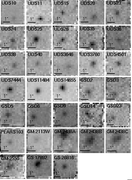
(a) UDSandGOODS-Sfields

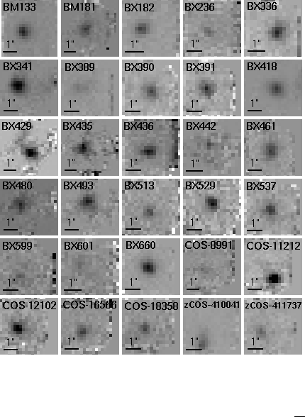
(b) Q2343andCOSMOSfields

Figure 1: Emission line images built from KMOS IFU H band data cubes for the UDS, GOODS-S, Q2343 and COSMOS fields. The images represent the [$\mathrm{O\ III}$]$\lambda$5007 line for objects at z $\sim$ 2.3 and H$\alpha$ for those at z $\sim$ 1.5. The number of wavelength slices used to construct the images depends on the intensity and width of the observed emission. The KMOS data cube for GMASS-2438 presents emission at three different positions inside the IFU FoV.

2 KMOS observations

Large databases, mostly cosmological fields, containing HIIG at high redshifts already exist in the literature so we have the possibility of selecting appropriate candidates with the specific requirements that we need for follow-up observations. The high number density of HIIG at high redshift allows the use of multi-object spectrographs reducing notably the amount of time required to build up a significant sample. The last column in Table LABEL:tab:table1, where we list the objects observed, gives the source for the selected candidates.

High spectral resolution near-IR spectra of 96 HIIG candidates were obtained using 55 hours of total observing time (PI R. Terlevich. Programmes 097.A-0039 and 098.A-0323) with the K-band Multi Object Spectrograph (KMOS; Sharples2013), a second-generation instrument at the Nasmyth focal plane of the VLT at ESO, which is able to perform simultaneous near-infrared Integral Field Spectroscopy for 24 targets.

2.1 Data description

The sample of 96 star-forming galaxies was selected from Erb2006a; Erb2006b; ForsterSchreiber2009; Mancini2011; van_der_Wel2011; Xia2012; Maseda2013; Maseda2014 following the criteria described in detail in GonzalezMoran2019. The candidates have high rest-frame equivalent width (EW) in their emission lines in a range of $1.2<$ z $<1.7$ and $1.9<$ z $<2.6$ in order to observe either H$\alpha$ or H$\beta$ and [$\mathrm{O\ III}$]$\lambda$5007Å lines in the H band and with the objects being in dense enough fields so that at least 10 of them would fit in the field of view (FoV) of the spectrograph.

KMOS is equipped with 24 integral field units (IFUs) that can be deployed by robotic arms to positions within the patrol field of 7.2′ in diameter. Each IFU has a square FoV of 2.8″ x 2.8″ sampled spatially at 0.2″ whilst maintaining Nyquist sampling ($\sim$ 2 pixel) of the spectral resolution element at the detector.

It provides a wavelength coverage of 1.456 - 1.846 $\mu$m in the H band at the FoV centre and achieves a spectral resolution of R = 4,000 in the atmospheric band. Due to spectral curvature, the IFUs at the edges of the array have a slightly different wavelength coverage than those at the centre.

We allocated the pick-off arms to specific targets in the patrol field using the KMOS Arm Allocator (KARMA; Wegner2008), an automated tool that optimises the assignments taking into account target priorities and mechanical constraints for the arms reach.

The data were obtained in service mode from June 2016 to July 2017 for period 97A with a total of 16 Observing Blocks (OBs) distributed in 2 fields on the cosmological field Q2343 (Steidel2004; Erb2006a; Erb2006b) and from December 2016 to October 2017 for the 98A period, distributed in 5 FoV on 3 cosmological fields: the Ultra Deep Survey (UDS; Lawrence2007; Cirasuolo2007), GOODS-South Deep (GSD; Giavalisco2004) and the Cosmic Evolution Survey (COSMOS; Scoville2007; Koekemoer2007), each OB with $\sim$ 40 minutes exposure time.

The observing mode adopted was ‘nod to sky’. Here, the 24 targets are observed in every pair of pointings with most of the arms on targets at the first position and the remainder on targets during the second exposure after a nod. In this case, the sky background is removed simply by subtracting alternate exposures for each arm. The data for each IFU are processed independently.

The observed sample is presented in Table LABEL:tab:table1. The target name is given in the first column, the coordinates in the second and third columns, the cosmological field that each object belongs to in column 4, the seeing in arcseconds corrected by airmass during the field observations in column 5, the total exposure time per target in seconds in column 6, and the reference from where the candidates were selected in column 7.

2.2 Data Reduction

The sample from the Q2343 field was observed in two overlapping FoV, 16 OBs for 8 repeated targets and 8 OBs for the rest. Five FoV were observed during the 98A period. Two FoV with 8 OBs each for the UDS field, two FoV with 8 OBs and 7 OBs for the GOODS-S field and one FoV with 8 OBs for the COSMOS field. In total 55 OBs with different position angles and 5 exposures each were observed. The total exposure time per target is shown in Table LABEL:tab:table1.

The data reduction was carried out via the KMOS Reflex workflow software (Freudling2013) developed by ESO and the instrument consortia (Davies2013). The software corrects the frames for their dark level and structure, flat-field, computes a wavelength solution, applies an illumination correction, a standard star flux calibration and telluric correction, and finally creates a cube reconstruction of the science data.

In order to guarantee the same orientation in all exposures for each FoV combination, we used ‘kmo rotate’ inside the ESO Recipe Execution tool, EsoRex for each exposure of the OBs per FoV.

By design, the KMOS workflow combines only the 5 exposures associated to a single OB, so we reduced all the OBs separately and then executed ‘kmo combine’ inside EsoRex.

The 1D spectrum extraction was made using the fits file viewer QFitsView (Ott2012) developed at the Max Planck Institute for Extraterrestrial Physics (MPE) and included in ESO’s SciSoft releases. This software allows to see in real time integrated spectra from different groups of spaxels of the KMOS data cube on the displayed image of the spatial FoV.

Table 1: Description of the analysed sample.

Sample	Description	N
S1	Observed KMOS sample	96
S2	S1 with emission lines detection	61
S3	S2 with enough S/N	54
S4	S3 with $\log\sigma-\epsilon_{\log\sigma}\leq$1.83	41
S5	S4 joint with linking data (see §3.3)	29

Figure 2: H$\alpha$ line for Q2343-BM133. The grey line is the spectrum, the dashed dark line is the Gaussian fit to the emission line and the box underneath shows the residuals. The inset at the upper right corner is the Monte Carlo analysis performed to the line where the standard deviation of the resulting distribution is taken as the uncertainty of the measured FWHM of the Gaussian fit.

3 Analysis

Emission lines were detected in 61 (sample S2; see Table 1) of the 96 HIIG candidates (sample S1) observed. Emission line images of the S2 objects are shown in Fig. 1, where there are 63 images instead of 61 because the data cube for GMASS-2438 presents emission at three different positions inside the IFU FoV. The images were built from the combination of slices within the particular wavelength range where the emission line was detected in the data cube. Note that most of them have sub arcsecond diameters and appear to be single.

One possible reason for the non detections is that the redshift range of the candidates, selected from their photometric redshift and with high [$\mathrm{O\ III}$] equivalent width, is wider than the KMOS line detection window. We adopted the strategy that if no emission lines were detected in a single exposure, then even if emission was detected in the complete exposure time the S/N would not be sufficient to determine the line width with the needed accuracy. So, we proceeded to inspect all single exposure spectra to identify those with a clear emission detection. The seven objects with the lowest S/N were removed from the S2 sample, the remaining 54 objects form the sample S3.

As in our group’s previous work, we have selected only those HIIG that have a logarithmic velocity dispersion ($\log\sigma-\epsilon_{\log\sigma}\leq$1.83), which minimises the probability of including rotationally supported systems, leaving 41 objects, sample S4 (see §3.1 for the velocity dispersion measurements). Finally, joining KMOS data with previous ones (obtained with MOSFIRE@Keck and XShooter@VLT, see §3.3), we ended up with 29 new HIIG (S5) that are added to the total sample for the cosmological analysis (see §4 and Table LABEL:tab:redshift,sigma_and_fluxes).

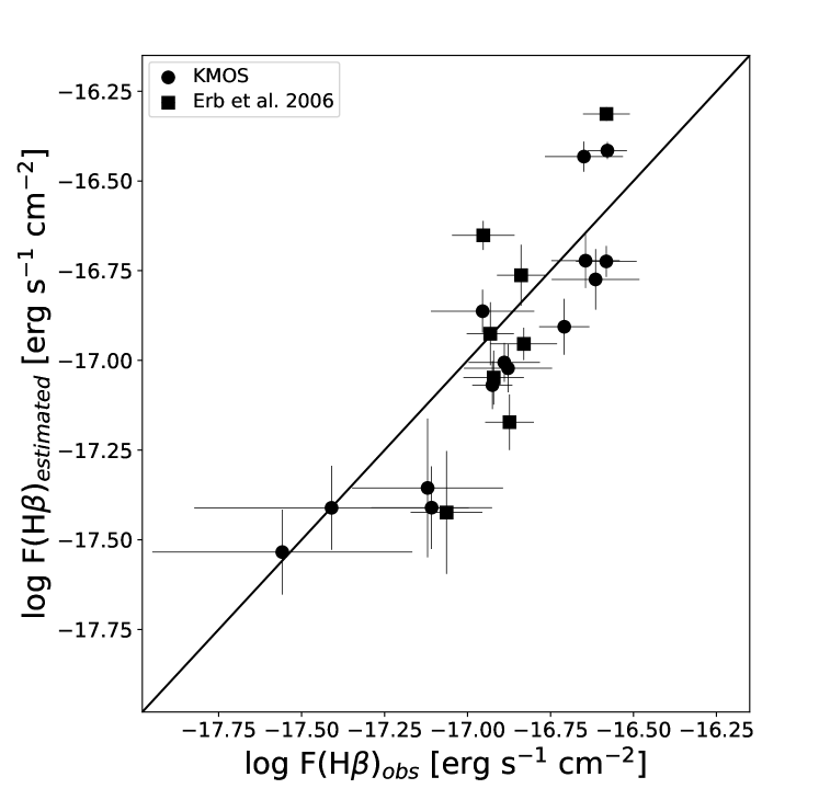
Figure 3: F(H$\beta$) estimated (from F([$\mathrm{O\ III}$]), see text) versus measured. The line represents the one-to-one relation.

3.1 Emission line widths

We determine the 1D velocity dispersion ($\sigma$) by fitting a Gaussian profile to each emission line ($\sigma_{obs}$) and subtracting in quadrature the thermal ($\sigma_{th}$), instrumental ($\sigma_{i}$) and fine structure broadening ($\sigma_{fs}$) components as:

$$\sigma^{2}=\sqrt{\sigma^{2}_{obs}-\sigma_{th}^{2}-\sigma_{i}^{2}-\sigma_{fs}^{2}}.$$ (1)

The uncertainty in $\sigma$ was estimated using the standard procedure for error propagation with independent errors (see e.g. Wall2012). The uncertainty in $\sigma_{obs}$ was estimated using a Monte Carlo analysis where a set of random realisations of each spectrum was generated using the r.m.s. intensity of the continuum adjacent to the emission line. The full width at half-maximum of the emission line (FWHM) 1$\sigma$ uncertainty was estimated from the standard deviation of the distribution of FWHM measurements.

Fig. 2 shows an example of the fit to the observed H$\alpha$ line and the distribution of FWHM obtained from the Monte Carlo simulations (in the inset) for the target Q2343-BM133. The residuals are shown in the bottom panel.

For the thermal broadening and the fine structure width we adopted the same values as in GonzalezMoran2019. The thermal broadening was calculated assuming a Maxwellian velocity distribution of the hydrogen and oxygen ions for which a reasonable value for the electron temperature ($T_{e}$) is $T_{e}=10,000$ K. The instrumental broadening was measured from the width of unsaturated and unblended sky lines.

Due to differences of instrumental resolution in each IFU and along the wavelength axis (Davies2013), there is a variation of the spectral resolution across all 24 IFUs. A unique value for the resolution is derived for each object depending on which IFU and at which wavelength the lines are observed.

We chose to perform the measurements inside the science IFU (instead of the sky one) because our targets are point-like sources (FWHM $<$ 1″) compared to the IFU FoV (2.8″$\times$ 2.8″). Hence the instrumental resolution is derived from the mean FWHM of OH sky emissions surrounding the line of interest. The instrumental resolution uncertainty was calculated using [max(FWHM)$-$min(FWHM)]$/2\sqrt{N}$, where max(FWHM) and min(FWHM) are the maximum and minimum FWHM of the set of measured sky lines and $N$ is the number of measurements. The instrumental resolution derived for each object is listed in column 6 of Table LABEL:tab:Observational_data.

Line widths are measured from either H$\alpha$ or H$\beta$ for the sample at z $<$ 2, and from [$\mathrm{O\ III}$]$\lambda$5007Å for the objects at z $>$ 2. Several groups (e.g. Hippelein1986; Bordalo_Telles2011; Bresolin2020) have found that the Balmer lines in HIIG and GHIIR are systematically broader than the [$\mathrm{O\ III}$]$\lambda$5007 Å. In order to bring both measurements into a single system, we corrected the [$\mathrm{O\ III}$]$\lambda$5007Å velocity dispersion measurements using the relation $\sigma$(H$\alpha$) = $\sigma$[$\mathrm{O\ III}$] + (2.91 $\pm$ 0.31) km s${}^{-1}$ determined for the local sample of HIIG from Chavez2014.

3.2 Fluxes

The emission line fluxes and EW were measured using the IRAF task splot and their uncertainties were estimated from the usual expressions (see e.g. Tresse1999) as in GonzalezMoran2019. Due to sky variations in the H band, a slightly negative residual background can appear after sky subtraction in the final spectra which needs to be corrected for. The correction consists of a constant offset to set to zero the residual background levels in the final 1D spectra. The background levels are estimated from the r.m.s continuum taken from windows that are clean of sky lines. The difference in flux with and without this correction is added as an uncertainty to the estimated flux as:

$$\epsilon_{Flux}=\sqrt{\epsilon^{2}_{F}+\epsilon^{2}_{backF}},$$ (2)

where $\epsilon_{F}$ was calculated following Tresse1999 and $\epsilon_{backF}$ is the uncertainty due to the residual background level.

Thirteen objects show only [$\mathrm{O\ III}$]$\lambda$5007Å  in the observed spectrum. For 9 of these Erb2006a published the value of F(H$\alpha$) and we calculated F(H$\beta$) from the theoretical F(H$\alpha$)/F(H$\beta$) ratio (2.86) expected for Case B recombination (Osterbrock1989) with $T_{e}=10,000$ K and low densities (N${}_{e}<100$ cm${}^{-3}$) and assuming the mean extinction that will be discussed in §3.4. For the remaining 4 objects, the F([$\mathrm{O\ III}$]) was transformed to F(H$\beta$) using the mean ratio F([$\mathrm{O\ III}$])/F(H$\beta$) obtained for our local sample of HIIG (Chavez2014).

In order to check the reliability of this method, we compared the measured F(H$\beta$) with F([$\mathrm{O\ III}$]) for those objects with both measurements, and the comparison is shown in Fig. 3. Based on this comparison, we kept the four objects for which we have only F([$\mathrm{O\ III}$]) in the analysis.

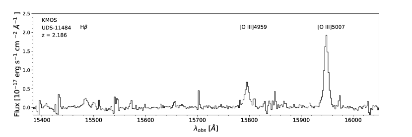
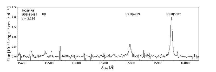
Figure 4: UDS-11484 1D spectra. Top panel: KMOS observations with a total exposure time of 9,400 seconds. Bottom panel: MOSFIRE observations with a total exposure time of 7,200 seconds. Both spectra have similar S/N per unit time and unit wavelength.

3.3 Repeated observations: KMOS, MOSFIRE, XShooter

With the intention of linking data obtained at different sites, with different instruments and telescopes, we observed with KMOS some objects from our previous samples. Twelve objects had previously been observed with MOSFIRE@Keck and XShooter@VLT with higher spectral resolution in the H band [R(MOSFIRE) $\sim$ 5400 and R(XShooter) $\sim$ 8000 against R(KMOS) $\sim$ 4000]. We chose to use the velocity dispersion for these objects from the higher dispersion data published in Terlevich2015 and GonzalezMoran2019.

The nine objects in common with MOSFIRE are UDS23, UDS25, UDS40, UDS-11484, UDS-14655, UDS-4501, COSMOS-16566, COSMOS-18358 and zCOSMOS-411737. In Fig. 4 we show an example of the spectra obtained for the same object (UDS-11484 at z=2.186) with KMOS and MOSFIRE in the region covering [$\mathrm{O\ III}$]$\lambda\lambda$4959, 5007Å and H$\beta$. Both spectra have similar S/N per unit time and unit wavelength. The three targets previously observed with XShooter are Q2343-BM133, Q2343-BX418 and Q2343-BX660.

Fig. 5 shows the comparison between the velocity dispersion determined from either H$\alpha$, H$\beta$ or [O III]$\lambda$5007Å for the targets with repeated observations in KMOS and XShooter (blue circles) or in KMOS and MOSFIRE (black circles). The target UDS-11484 at z=2.2 appears twice (black squares) as its $\sigma$ was measured from both H$\beta$ and [$\mathrm{O\ III}$].

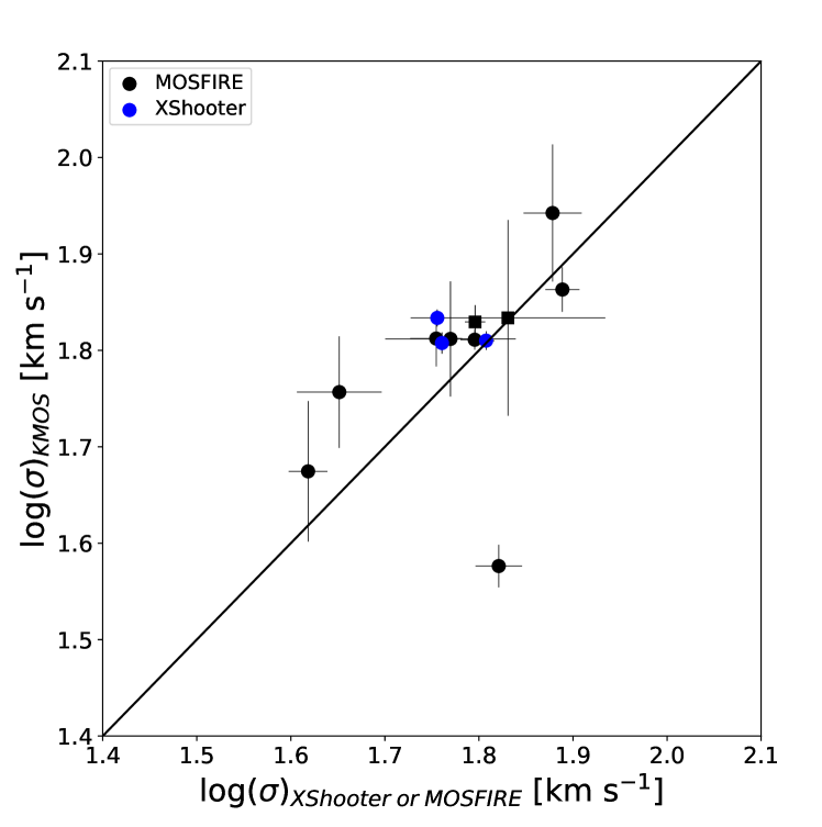
Figure 5: Comparison between the velocity dispersion from MOSFIRE or XShooter and KMOS data. The solid line represents the one to one relation. The two squares correspond to UDS-11484 for the velocity dispersion determined from either H$\beta$ or [O III]$\lambda$5007Å. The largest error bars correspond to the H$\beta$ value. The outlier is COSMOS-18358.

We can see from Fig. 5 that the measurements are in agreement within 1$\sigma$ except for the outlier source COSMOS-18358. In order to understand this discrepancy, we compare its KMOS and MOSFIRE 1D and 2D spectra (see Fig. 6). To extract the 2D KMOS spectrum, a pseudo-longslit from the data cube was created using the function longslit in QFitsView. It is clear from the figure that for this object, the sky subtraction for the MOSFIRE spectrum is better than for the KMOS one for which a sky emission line coincides with H$\alpha$. From the redshifts measured in both spectra, we find that z${}_{MOSFIRE}$ is slightly lower than z${}_{KMOS}$ (1.6492 vs 1.6494) which confirms that the blue side of H$\alpha$ in the KMOS spectrum is affected by a bad subtraction of a sky emission line. In consequence, considering also the better spectral resolution of the MOSFIRE data, we use in what follows the velocity dispersion calculated from the MOSFIRE spectra whenever possible.

Fig. 7 shows the redshift difference $\Delta$z for the targets with either MOSFIRE or XShooter previous observations. The mean of $\Delta$z is 4$\times$10${}^{-4}$ and as individual redshift uncertainties given by the Gaussian fit to the emission lines are of the order of 10${}^{-5}$, we set the redshift uncertainty for the KMOS and MOSFIRE data to 4$\times$10${}^{-4}$ for a more realistic value.

$\begin{array}[]{cc}\vspace{-1cm}{\includegraphics[width=260.17464pt]{fig/COSMOS18358_KMOS_v2_f.pdf}}&{\includegraphics[width=261.47147pt]{fig/COSMOS18358_MOSFIRE_v2_f.pdf}}\end{array}$

Figure 6: COSMOS-18358 2D (top) and 1D (bottom) spectra. Left panel: KMOS data with a total exposure time of 9 800 seconds. Right panel: MOSFIRE data with a total exposure time of 10 080 seconds.

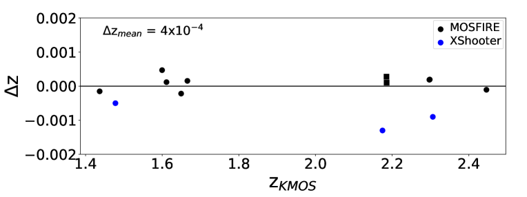
Figure 7: $\Delta$z: redshift difference for the targets observed with MOSFIRE or XShooter and with KMOS compared to the value obtained from KMOS data.

The KMOS IFU FoV (2.8″$\times$ 2.8″) ensures that there is virtually no flux loss for the high redshift HIIG (which are smaller than 1″, see Fig. 1). This was not the case for the MOSFIRE observations (GonzalezMoran2019) where a slit width of 0.48″was used. A comparison of the flux for the 9 targets observed with both instruments provides an estimate of the slit loss which is henceforth used to correct the fluxes measured from the MOSFIRE data. This is shown in Fig. 8 where the continuous line is the linear fit obtained using the mpfit routine. Note that, as in Fig. 5, there are 10 points instead of 9 in the figure for the two velocity dispersion values obtained using H$\beta$ and [$\mathrm{O\ III}$]$\lambda$5007Å in UDS-11484. Even though there is not much difference between MOSFIRE and KMOS fluxes, we corrected the MOSFIRE sample fluxes for slit loss. The results are shown in Table LABEL:tab:redshift,sigma_and_fluxes.

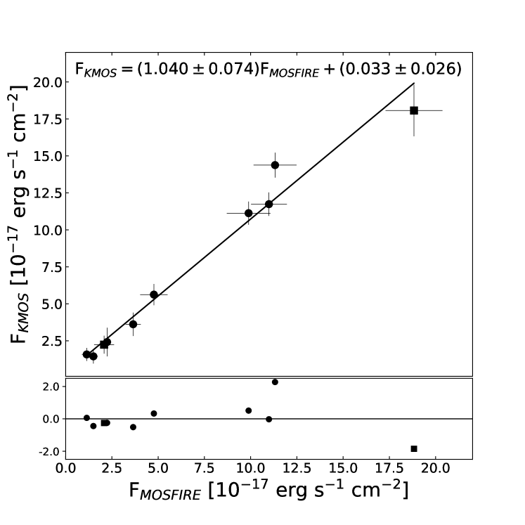
Figure 8: Fluxes measured in repeated observations with MOSFIRE vs. KMOS. The black line is the fit and the box underneath shows the residuals.

3.4 Extinction correction

Extinction correction was determined using the Gordon2003 extinction law chosen because the dust attenuation curves derived from analogs of high redshift star forming galaxies by Salim2018 and from star forming galaxies at z $\sim$ 2 by Reddy2015 are in good agreement with the LMC and SMC curves given by Gordon2003 (see Fig. 3 from GonzalezMoran2019).

The extinction corrected fluxes were determined as usual from the expression:

$$F(\lambda)=F_{obs}(\lambda)10^{0.4\textsc{Av}k(\lambda)/\textsc{Rv}},$$ (3)

where $k(\lambda)=A(\lambda)/E(B-V)$ is given by the extinction law used. We adopt $k(H\beta)=3.33$ and $k(H\alpha)=2.22$ and Rv = 2.77 (Gordon2003).

Given the objects redshift, we cannot measure the Balmer decrement from the H band data. We adopted instead the mean extinction (Av=0.71$\pm$0.13) derived for our local sample (Chavez2014).

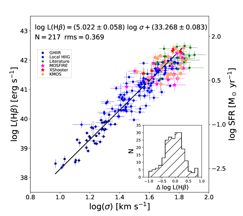
Figure 9: $L-\sigma$ relation for the Global sample (see Table 2) using the Gordon2003 extinction curve. The right axis shows the SFR estimated from the L(H$\beta$) using SFR$=1.54\times 10^{41}$L(H$\beta$). The black line is the fit, obtained only from the local samples, shown at the top and the lower right corner box shows the residuals.

4 Results

For cosmological parameter analysis we include both our new KMOS data and previously published samples of low- and high-z targets. This is summarised in Table 2, where the first column gives the reference name of the sample, the second lists its description and the third gives the number of objects in each subsample.

The $L-\sigma$ relation shown in Fig. 9 includes the new data for high-z objects presented in §2, in addition to the sample in GonzalezMoran2019, giving a total of 74 high-z HIIG. The intercept ($\alpha$) and slope ($\beta$) of the relation, shown in the figure inset, are estimated for the sample of 107 local ($0.01\leq z\leq 0.15$) HIIG published in Chavez2014 and 36 GHIIR at z $\leq 0.01$ described in Fernandez2018 using the Gordon2003 extinction curve. We use the values of $\alpha$ and $\beta$ so obtained as the nuisance parameters of the $L-\sigma$ relation unless stated otherwise. Fig. 10 shows the Hubble diagram for the Global sample of 217 objects at $0.01\leq z\leq 2.6$ (see Table 2) where the redshift range covered by our data can be clearly appreciated.

Table 2: Samples used in the cosmological analysis.

Sample	Description	N
KMOS	S5 sample	29
MOSFIRE	MOSFIRE sample corrected by slit loss flux	15
XShooter	XShooter sample corrected by slit loss flux	6
Literature	Literature sample${}^{a}$	24
High-z	KMOS + MOSFIRE + XShooter + Literature	74
Local	Local HIIG sample	107
Full	High-z + Local	181
Our data	Full excluding Literature	157
GHIIR	GHIIR sample	36
Global	Full + GHIIR	217
${}^{a}$ Erb2006a; Masters2014 and Maseda2014.

4.1 Cosmological parameters constraints

To constrain cosmological parameters in a way that is independent of $h$, we follow the methodology from our previous work (Chavez2016; GonzalezMoran2019) which we summarise in what follows.

The likelihood function for HIIG and GHIIR is given as:

$$\mathcal{L}_{HII}\propto\exp{(-\frac{1}{2}\chi^{2}_{HII})},$$ (4)

where:

$$\chi^{2}_{HII}=\sum_{n}\frac{(\mu_{o}(\log f,\log\sigma|\alpha,\beta)-\mu_{\theta}(z|\theta))^{2}}{\epsilon^{2}},$$ (5)

and $\mu_{o}$ is the distance modulus calculated from the observables, $\mu_{\theta}$ is the theoretical distance modulus, $\alpha$ and $\beta$ are the $L-\sigma$ relation’s intercept and slope respectively; $\sigma$ is the broadening corrected velocity dispersion and $f$ is the extinction corrected flux.

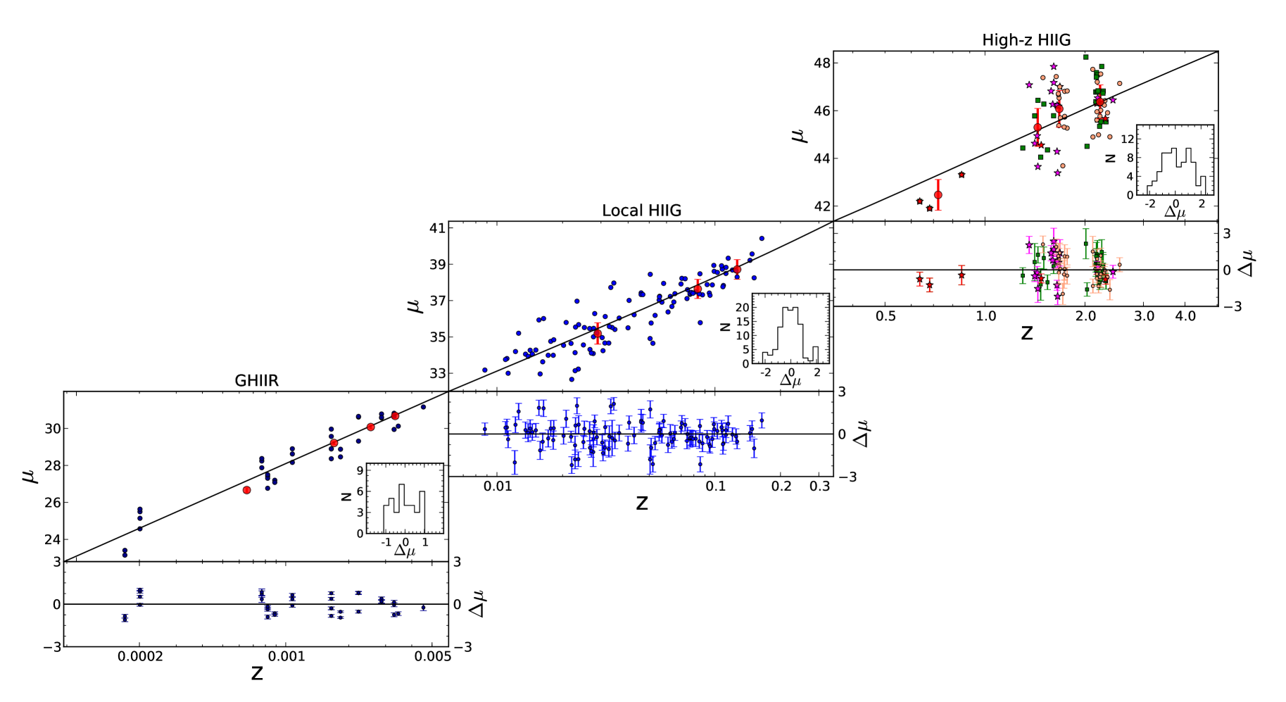
Figure 10: Hubble diagram connecting our local and high redshift samples up to z $\sim$ 2.6. Red circles represent averages of the distance moduli in redshift bins; the rest of the symbols are as in Fig. 9. The continuous line corresponds to $\Omega_{m}=0.249$ and $w_{0}=-1.18$ (our best cosmological model using only HIIG, see §4.1.2). The insets show the distribution of the residuals of the fit that are plotted in the bottom panels.

The theoretical distance modulus $\mu_{\theta}$ in Eq. 5 depends on a set of cosmological parameters, in the most general case considered here given as $\theta=\{h,\Omega_{m},w_{0},w_{a}\}$, and the redshift ($z$). The parameters $w_{0}$ and $w_{a}$ refer to the DE EoS, the general form of which is:

$$p_{w}=w(z)\rho_{w}c^{2}\;,$$ (6)

with $p_{w}$ the pressure and $\rho_{w}$ the density of DE, while $w(z)$ is an evolving DE EoS parameter. There are different DE models, many are parametrized using a Taylor expansion around the present epoch like the CPL model (Chevallier2001; Linder2003; Peebles2003; Dicus2004; Wang2006) in which:

$$w(z)=w_{0}+w_{a}\frac{z}{1+z}\;,$$ (7)

The cosmological constant is just a special case of DE, given for $(w_{0},w_{a})=(-1,0)$, while the so called wCDM models are such that $w_{a}=0$ but $w_{0}$ can take values $\neq-1$.

Finally $\epsilon^{2}$, the weights in the likelihood function, can be given as:

$$\epsilon^{2}=\epsilon^{2}_{\mu_{o},stat}+\epsilon^{2}_{\mu_{\theta},stat}+\epsilon^{2}_{sys},$$ (8)

where $\epsilon_{\mu_{o},stat}$ are the statistical uncertainties given as:

$$\epsilon^{2}_{\mu_{0},stat}=6.25(\epsilon_{\log f}^{2}+\beta^{2}\epsilon_{\log\sigma}^{2}+\epsilon_{\beta}^{2}\log\sigma^{2}+\epsilon_{\alpha}^{2}).$$ (9)

$\epsilon_{\log f}$, $\epsilon_{\log\sigma}$, $\epsilon_{\alpha}$ and $\epsilon_{\beta}$ are the uncertainties associated with the logarithm of the flux, the logarithm of the velocity dispersion and the intercept and slope of the $L-\sigma$ relation respectively, while $\epsilon_{\mu_{\theta},stat}$ in Eq. 8 is the uncertainty associated with the distance modulus as propagated from the redshift uncertainty in the case of HIIG and as given by the primary distance indicator measurement uncertainty for the case of GHIIR. $\epsilon_{sys}$ are the systematic uncertainties that will be briefly discussed in §4.2 and in more detail in a forthcoming paper (Chávez et al., in prep).

It is convenient to define also an $h$-free likelihood function (cf. Nesseris2005) through a rescaling of the luminosity distance ($d_{L}$) given by:

$$D_{L}(z,\theta)=(1+z)\int_{0}^{z}{\frac{dz^{{}^{\prime}}}{E(z^{{}^{\prime}},\theta)}}\;,$$ (10)

i.e., $d_{L}=cD_{L}/H_{0}$. We use this rescaling to constrain cosmological parameters in an $h$ independent way as fully described in GonzalezMoran2019.

The $L-\sigma$ relation has been used in the local Universe to constrain the value of $h$ (Chavez2012; Fernandez2018). The main objective of this work is to constrain the parameters $\theta=\{\Omega_{m},w_{0},w_{a}\}$ in a way that is independent of $h$. However, we will also constrain $h$ in some cases, using the full likelihood function as given in Eq. 4 in order to compare our results with the literature. For each result we will specify whether or not it is independent of $h$ and which parameters have been left fixed.

Unless otherwise stated, we use the MultiNest Bayesian inference algorithm (cf. Feroz2008; Feroz2009; Feroz2013), to maximise the likelihood function and get constraints to the different combinations of nuisance and cosmological parameters. In all the cases we use the priors given in Table 3 (Chavez2016).

Table 3: Priors for Constrained Parameters.

Parameter	Prior
Cosmological Parameters
$h$	Uniform [0.5, 1.0]
$\Omega_{m}$	Uniform [0.0, 1.0]
$w_{0}$	Uniform [$-$2.0, 0.0]
$w_{a}$	Uniform [$-$4.0, 2.0]
$w_{b}$	Uniform [0.0, 0.05]
HIIG Nuisance Parameters
$\alpha$	Uniform [32.5, 34.5]
$\beta$	Uniform [4.5, 5.5]

4.1.1 Constraining $\Omega_{m}$

Applying the $h$ independent method described above to the joint local and high-$z$ sample of 181 HIIG (dubbed the Full sample in Table 2), and assuming the standard $\Lambda$CDM model with $w_{0}=-1$, we find $\Omega_{m}=0.236^{+0.047}_{-0.041}$ (stat) and $\Omega_{m}=0.244^{+0.040}_{-0.049}$ (stat) for the $\chi^{2}$-minimisation procedure and the MultiNest MCMC, respectively. The last result is also shown in Table 4. If we restrict the sample to the 157 HIIG observed by our group (i.e excluding the data taken from the literature, Our data in Table 2), we obtain $\Omega_{m}=0.243^{+0.047}_{-0.057}$ (stat); the posterior for this case is shown in Table 5.

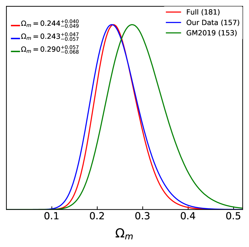
Figure 11: Comparison between the $\Omega_{m}$ posterior for our current HIIG sample with and without data from the literature (Full and Our Data, respectively) and that of GonzalezMoran2019. The number of objects in each sample is shown between parentheses.

For the purpose of comparing our current constraints with other determinations, we adopt the definition of figure of merit ($FoM$) given by Wang2008:

$$FoM=\frac{1}{\sqrt{det\ Cov(\theta_{0},\theta_{1},\theta_{2},...)}}\,$$ (11)

where $Cov(\theta_{0},\theta_{1},\theta_{2},...)$ is the covariance matrix of a set of parameters $\{\theta_{i}\}$.

Our current constraints can be compared with the value of $\Omega_{m}=0.290^{+0.056}_{-0.069}$ (stat) ($FoM=16.01$) for the sample of 153 objects (GonzalezMoran2019), which includes the Literature sample. We find an improvement of the cosmological parameter constraints by 21% using Our data sample ($FoM=19.38$) or by 37% when considering the Full sample ($FoM=22.0$). We also compare the posteriors for these three different cases in Fig. 11.

The comparison of our value for $\Omega_{m}$ with other results from the literature is summarised in Fig. 12 where dashed error bars denote statistical and systematic uncertainties and continuous error bars, only statistical. The shaded region (given as a visual aid) represents the uncertainties of our current $\Omega_{m}$ value.

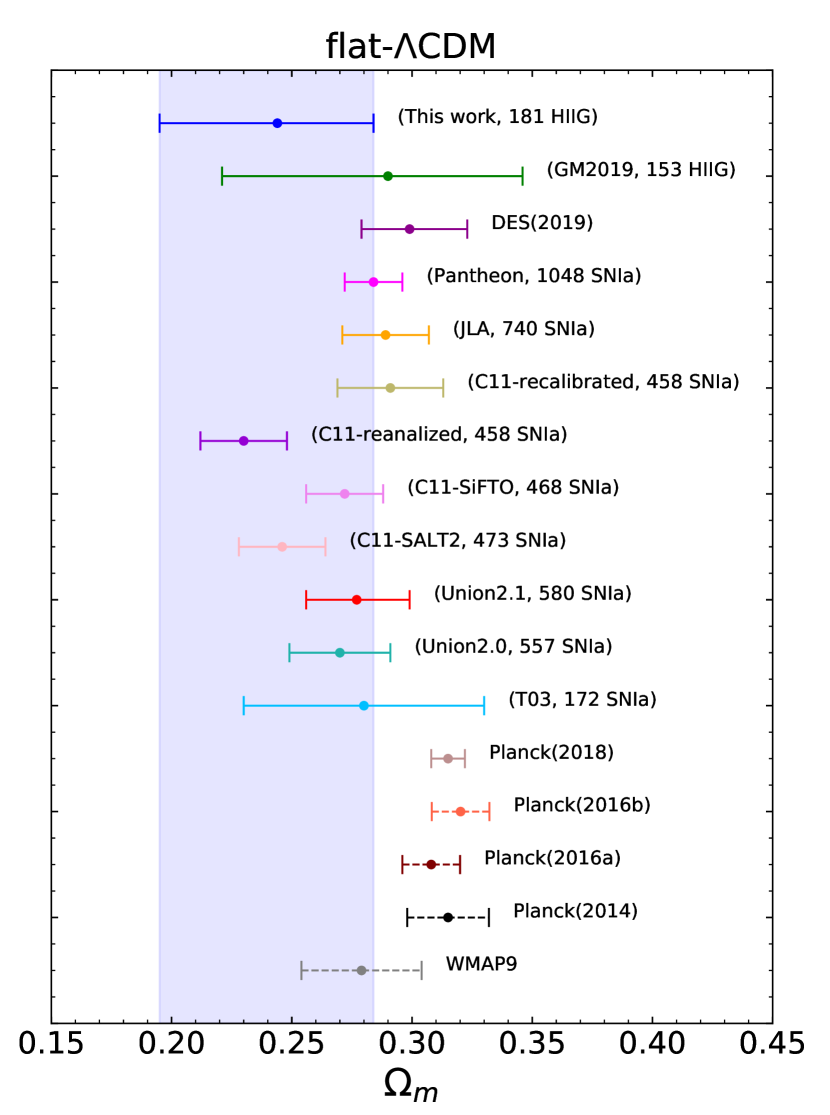
Figure 12: Comparison of our $\Omega_{m}$ value for the Full sample with literature results. The number of objects and the distance estimator in each sample are shown in parentheses. The continuous error bars are the statistical uncertainties; dashed ones represent both statistical plus systematic uncertainties. The shaded region represents the uncertainties of our current $\Omega_{m}$ value.

Our result is in agreement with the CMB determination from WMAP9 (Bennett2013) of $\Omega_{m}=0.279\pm 0.025$ at a $<1\sigma$ level. It is in disagreement with those found by PlanckCollaboration2016a; PlanckCollaboration2016b; PlanckCollaboration2018 of $\Omega_{m}=0.308\pm 0.012$, $\Omega_{m}=0.320\pm 0.009$ (stat) and $\Omega_{m}=0.315\pm 0.007$ (stat + sys) by 1.4, 1.7 and 1.6$\sigma$, respectively, although we are only considering random errors and the Planck collaboration included systematics.

Our determination of $\Omega_{m}$ is also in agreement with the result from the Dark Energy Survey (DES) collaboration of $\Omega_{m}=0.299^{+0.024}_{-0.020}$ (Abbott2019) which results from the joint analysis of BAO, SNIa, weak lensing and galaxy clustering.

As systematic uncertainties for the HIIG sample are not included in the present analysis, it is interesting to compare with the results presented by Betoule2014, who analyse the drift on the value of $\Omega_{m}$ (and SNIa analysis nuisance parameters) with respect to the results presented by Conley2011, considering statistical uncertainties only. They found $\Omega_{m}=0.246\pm 0.018$ (stat) and $\Omega_{m}=0.272\pm 0.016$ (stat), for the C11 sample analysis using the SALT2 (Guy2007) and SiFTO (Conley2008) light-curve models respectively. Betoule2014 recalibrated the C11 sample and found $\Omega_{m}=0.291\pm 0.022$ (stat) for 458 SNIa which is in agreement with their value of $\Omega_{m}=0.289\pm 0.018$ (stat) for the JLA sample of 740 SNIa. Our determination is compatible with both results.

As can be seen in Fig. 12, the size of the error bars for the SNIa based $\Omega_{m}$ largely depends on the number of targets used. For example, the High-z Supernova Search Team with 172 SNIa (Tonry2003) found $\Omega_{m}=0.28\pm 0.05$ (stat). From this result, we can conclude that for a comparable size of the sample used, our uncertainties are similar to those from SNIa. The two samples however span a different redshift range: up to 1.2 for Tonry2003 and up to 2.6 for ours. We aim at filling the gap seen between 0.2 $<$ z $<$ 1.2 in our Hubble diagram (Fig. 10) with forthcoming ground based observations.

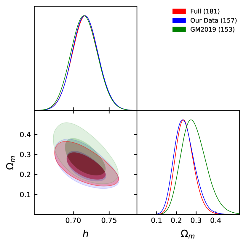
Figure 13: Confidence levels in the $\{h,\Omega_{m}\}$ plane for our current Full sample (Full), our sample excluding data from the literature (Our Data), and GonzalezMoran2019 sample (GM2019). The number of objects for each sample is shown in parentheses.

Using the full likelihood function as stated in Eq. 4, it is possible to constrain the $\{h,\Omega_{m}\}$ plane; in this case for our Full sample we obtain:

$h=0.717\pm 0.018$ (stat) and $\Omega_{m}=0.243^{+0.039}_{-0.050}$ (stat)

as reported in Table 4.

While using Our Data sample we obtain:

$h=0.717\pm 0.018$ (stat) and $\Omega_{m}=0.242^{+0.042}_{-0.057}$ (stat),

as reported in Table 5.

If we use the 153 HIIG from GonzalezMoran2019 to constrain the same model, we get:

$h=0.715\pm 0.018$ (stat) and $\Omega_{m}=0.290^{+0.052}_{-0.070}$ (stat),

comparing the $FoM$ of these last results with that one from the Full sample the relative improvement of the cosmological parameters constraints is $\sim 46\%$. In Fig. 13 we show a comparison for the three cases discussed above.

Reanalysing our sample from GonzalezMoran2019, Cao2020 also constrain the $\{h,\Omega_{m}\}$ plane for the $\Lambda$CDM model and they obtain:

$h=0.717\pm 0.018$(stat) and $\Omega_{m}=0.289^{+0.053}_{-0.071}$ (stat), which is consistent with our determination for the Full sample.

4.1.2 Constraining the dark energy equation of state

For comparison with previous works (e.g. GonzalezMoran2019), we get constraints in the $\{\Omega_{m},w_{0}\}$ plane using the classical $\chi^{2}$-minimisation and our results are: $\Omega_{m}=0.24^{+0.07}_{-0.06}$ (stat) and $w_{0}=-1.02^{+0.26}_{-0.37}$ (stat). Fig. 14 shows the $\chi^{2}$ likelihood contours corresponding to the 1$\sigma$ confidence level together with that from GonzalezMoran2019 (for 181 vs. 153 objects in the same wavelength range).

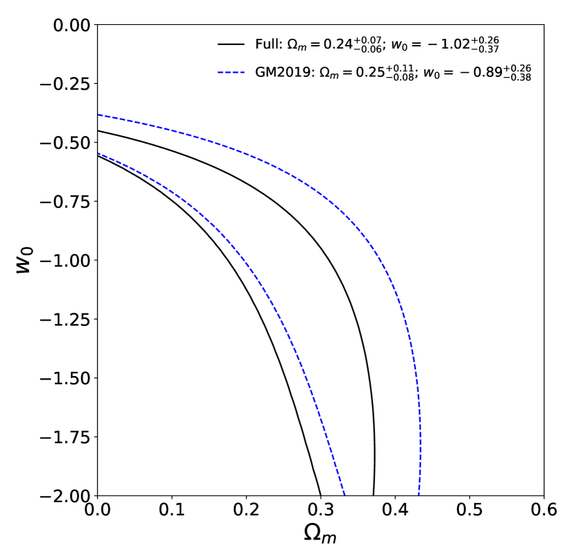
Figure 14: $\chi^{2}$ likelihood contours for $\Delta\chi^{2}=\chi^{2}_{tot}-\chi^{2}_{tot,min}$ equal to 2.30 corresponding to the 1$\sigma$ confidence level in the $\{\Omega_{m},w_{0}\}$ plane. The solid black line is for the Full sample and the dashed blue line is for the GM2019 one.

Applying the $h$-free likelihood trough the MultiNest Bayesian sampler, as described above, to constrain the parameters of the $w$CDM model, we obtain the marginalised best-fit parameter values and $1\sigma$ uncertainties in the $\{\Omega_{m},w_{0}\}$ plane for the Full sample. Our constraints are:

$\Omega_{m}=0.249^{+0.11}_{-0.065}$ (stat) and $w_{0}=-1.18^{+0.45}_{-0.41}$ (stat).

This result is presented also in Table 4 and the likelihood contours corresponding to the 1 and 2$\sigma$ confidence levels are shown in Fig. 15.

Following the same methodology for Our Data sample the results are:

$\Omega_{m}=0.246^{+0.11}_{-0.076}$ (stat) and $w_{0}=-1.16^{+0.46}_{-0.40}$ (stat),

which are also reported in Table 5. Comparing this determination with the results obtained in GonzalezMoran2019 and the $FoM$ as described above, the improvements on the cosmological parameters constraints are $\sim 31\%$ and $\sim 40\%$ for the Full sample.

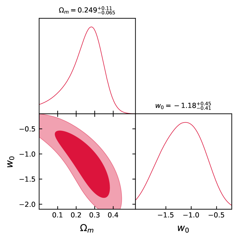
Figure 15: Likelihood contours corresponding to 1$\sigma$ and 2$\sigma$ confidence levels in the $\{\Omega_{m},w_{0}\}$ space for the Full sample.

Fig. 16 shows our constraints for the Full sample with other recent determinations for the $\{\Omega_{m},w_{0}\}$ plane. It is clear that our determination is fully consistent with the other results from local Universe probes, specifically SNIa. The best agreement is with the results from the JLA sample (Betoule2014), $\Omega_{m}=0.247^{+0.11}_{-0.064}$ (stat) and $w_{0}=-0.94^{+0.23}_{-0.16}$ (stat), and with the Union2.1 sample (Suzuki2012), $\Omega_{m}=0.281^{+0.067}_{-0.092}$ (stat) and $w_{0}=-1.011^{+0.208}_{-0.231}$ (stat). The results from the most recent Pantheon sample (Scolnic2018), $\Omega_{m}=0.350\pm 0.035$ (stat) and $w_{0}=-1.251\pm 0.144$ (stat), produce a considerably larger value for $\Omega_{m}$ than both previous SNIa samples and our own determination. Even so, we are still marginally consistent due partially to our large error bars. One point of interest is the big drift on the values for the $\{\Omega_{m},w_{0}\}$ plane from the JLA to the Pantheon SNIa samples, which may be interesting to explore.

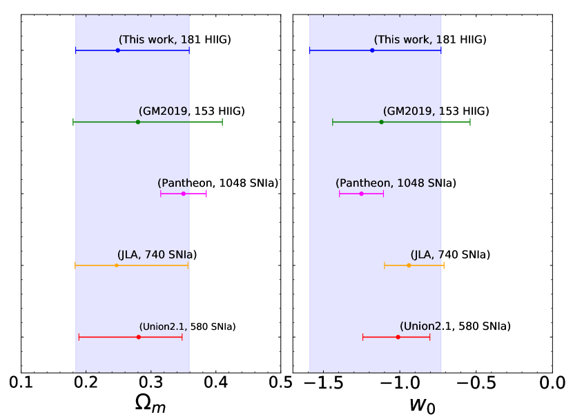
Figure 16: Comparison of our results for $\{\Omega_{m},w_{0}\}$ plane (Full HIIG sample) with the literature. Only statistical uncertainties are considered. As in Fig. 12, the shaded region represents the uncertainties of our current values.

As in the previous section, we also analyse the results from the full likelihood to constrain the $\{h,\Omega_{m},w_{0}\}$ plane. When we use the Full sample, our determination is $\{h,\Omega_{m},w_{0}\}=\{0.719\pm 0.020,0.250^{+0.10}_{-0.061},-1.19^{+0.46}_{-0.38}\}$ (stat) (Fig. 17 and in Table 4). Using Our Data sample, the result is $\{h,\Omega_{m},w_{0}\}=\{0.718\pm 0.020,0.245^{+0.11}_{-0.071},-1.16^{+0.50}_{-0.35}\}$ (stat).

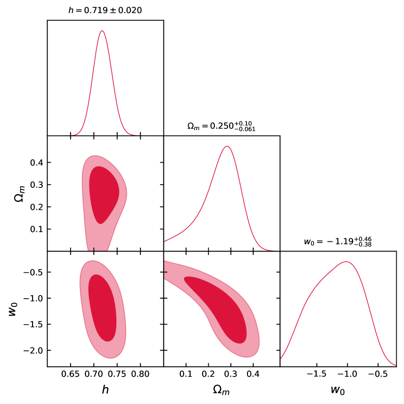
Figure 17: Likelihood contours corresponding to the 1$\sigma$ and 2$\sigma$ confidence levels in the $\{h,\Omega_{m},w_{0}\}$ space for the Full sample.

4.1.3 Nuisance and cosmological parameters simultaneous determination

A global fit of all the free parameters, nuisance and cosmological, applying the full likelihood to our Global sample (Table 2) provides the following results:

$\alpha$ = 33.24 $\pm$ 0.14, $\beta$ = 5.03 $\pm$ 0.12,

$h$ = 0.720 $\pm$ 0.040,

$\Omega_{m}=0.274^{+0.14}_{-0.079}$ , $w_{0}=-1.00^{+0.53}_{-0.26}$,

as reported in Table 4. In Fig. 18 we plot the 1 and 2$\sigma$ likelihood contours in the various parameter planes. From this result, it is clear that our determination of the global set of parameters is fully consistent with the previous determinations cited above and with other recent determinations. Comparing the $FoM$ of these results with those obtained in GonzalezMoran2019 the improvement is $\sim 52\%$.

Following the same methodology, we also present in Table 5 the results of excluding the Literature sample from the Global sample, i.e., for 193 objects.

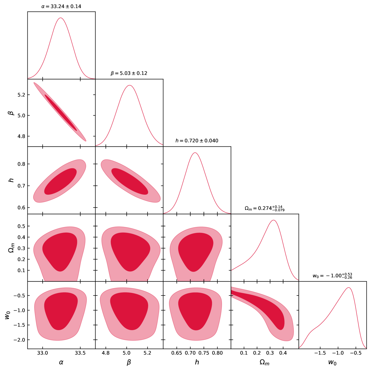
Figure 18: Likelihood contours corresponding to the 1$\sigma$ and 2$\sigma$ confidence levels in the $\{\alpha,\beta,h,\Omega_{m}\,w_{0}\}$ space for the Global sample.

Table 4: Marginalised best-fit parameter values and $1\sigma$ uncertainties for the HIIG sample, including data taken from the literature, and its combination with other samples. In parenthesis the fixed values.

Data Set	$\alpha$	$\beta$	$\omega_{b}$	$h$	$\Omega_{m}$	$w_{0}$	$w_{a}$	N	$\chi^{2}$
HIIG	—	($5.022\pm 0.058$)	—	—	$0.244^{+0.040}_{-0.049}$	(-1.0)	(0.0)	181	258.11
HIIG	—	($5.022\pm 0.058$)	—	—	$0.249^{+0.11}_{-0.065}$	$-1.18^{+0.45}_{-0.41}$	(0.0)	181	258.33
HIIG	($33.268\pm 0.083$)	($5.022\pm 0.058$)	—	$0.717\pm 0.018$	$0.243^{+0.039}_{-0.050}$	(-1.0)	(0.0)	181	258.10
HIIG	($33.268\pm 0.083$)	($5.022\pm 0.058$)	—	$0.719\pm 0.020$	$0.250^{+0.10}_{-0.061}$	$-1.19^{+0.46}_{-0.38}$	(0.0)	181	258.55
HIIG	$33.23\pm 0.14$	$5.04\pm 0.12$	—	$0.719\pm 0.040$	$0.313^{+0.046}_{-0.057}$	(-1.0)	(0.0)	217	785.12
HIIG	$33.24\pm 0.14$	$5.03\pm 0.12$	—	$0.720\pm 0.040$	$0.274^{+0.14}_{-0.079}$	$-1.00^{+0.53}_{-0.26}$	(0.0)	217	786.41
SNIa	—	—	—	—	$0.349^{+0.038}_{-0.029}$	$-1.25^{+0.15}_{-0.13}$	(0.0)	1048	1032.56
BAO	—	—	(0.02225)	(0.6774)	$0.306^{+0.035}_{-0.041}$	$-0.96^{+0.11}_{-0.14}$	(0.0)	6	1.76
CMB	—	—	$0.02225\pm 0.00016$	(0.6774)	$0.3107\pm 0.0029$	$-0.954\pm 0.020$	(0.0)	3	0.025
HIIG+CMB+BAO	—	($5.022\pm 0.058$)	(0.02225)	$0.693\pm 0.01$	$0.298\pm 0.012$	$-1.005\pm 0.051$	(0.0)	190	262.37
HIIG+CMB+BAO	—	($5.022\pm 0.058$)	(0.02225)	$0.698\pm 0.023$	$0.294^{+0.018}_{-0.021}$	$-1.07^{+0.23}_{-0.32}$	$0.16^{+0.96}_{-0.55}$	190	262.14
SNIa+CMB+BAO	—	—	(0.02225)	$0.6977\pm 0.0060$	$0.2940\pm 0.0057$	$-1.024\pm 0.022$	(0.0)	1057	1037.80
SNIa+CMB+BAO	—	—	(0.02225)	$0.6885\pm 0.0099$	$0.3011\pm 0.0085$	$-1.062\pm 0.040$	$0.25^{+0.22}_{-0.19}$	1057	1036.37

Table 5: Marginalised best-fit parameter values and $1\sigma$ uncertainties for our own HIIG sample. Fixed values in parenthesis.

Data Set	$\alpha$	$\beta$	$h$	$\Omega_{m}$	$w_{0}$	$w_{a}$	N	$\chi^{2}$
HIIG	—	($5.022\pm 0.058$)	—	$0.243^{+0.047}_{-0.057}$	(-1.0)	(0.0)	157	231.09
HIIG	—	($5.022\pm 0.058$)	—	$0.246^{+0.11}_{-0.076}$	$-1.16^{+0.46}_{-0.40}$	(0.0)	157	231.25
HIIG	($33.268\pm 0.083$)	($5.022\pm 0.058$)	$0.717\pm 0.018$	$0.242^{+0.042}_{-0.057}$	(-1.0)	(0.0)	157	231.10
HIIG	($33.268\pm 0.083$)	($5.022\pm 0.058$)	$0.718\pm 0.020$	$0.245^{+0.11}_{-0.071}$	$-1.16^{+0.50}_{-0.35}$	(0.0)	157	231.43
HIIG	$33.25\pm 0.14$	$5.02\pm 0.12$	$0.723\pm 0.041$	$0.322^{+0.049}_{-0.061}$	(-1.0)	(0.0)	193	733.41
HIIG	$33.25\pm 0.14$	$5.02\pm 0.12$	$0.723\pm 0.040$	$0.276^{+0.14}_{-0.091}$	$-0.98^{+0.55}_{-0.21}$	(0.0)	193	734.42

4.2 Systematic errors

In previous sections we have discussed the statistical uncertainties associated with our methodology. However, the scatter found in the $L-\sigma$ relation for HIIG suggests the presence of a second parameter probably associated with the line profile shape (Bordalo_Telles2011; Chavez2014) or/and systematic errors. Systematic uncertainties are difficult to estimate and in this section we will briefly discuss part of the systematic errors that can be included in the likelihood function (Eq. 8).

Not knowing the shape of the extinction law for HIIG and its possible variation with redshift is an important source of uncertainty. We have found GonzalezMoran2019 that when applying to the data a correction based on the Calzetti2000 law, we obtain a smaller reduced $\chi^{2}$ (1.1) than when we apply the Gordon2003 correction (1.7). However, Calzetti’s law was derived from a sample of eight heterogeneous starburst galaxies where only two, Tol 1924-416 and UGCS410 are bonafide HIIG and the rest are evolved high metallicity starburst galaxies, while Gordon2003 extinction curve corresponds to the LMC supershell near the 30 Doradus star forming region, the prototypical GHIIR. Besides, as already mentioned in §3.4, the dust attenuation curve derived from analogues of high-redshift star-forming galaxies agrees quite well with Gordon2003. Therefore, we prefer the results using Gordon’s extinction curve.

A related source of uncertainty is associated with the fact that we do not have extinction estimates for individual HIIG with $z\geq 1$ and for these systems we have adopted the average extinction of the low-z HIIG assuming that there is no systematic variation associated with redshift. A welcome improvement would be to obtain the Balmer decrement for the high-z sample.

In Chavez2016 we presented a systematic error budget on the distance moduli of 0.257. This includes the typical uncertainty contribution from the size and age of the burst, abundances and extinction. Adding in quadrature this systematic error budget in Eq. 8, we obtain a reduced $\chi^{2}$ close to 1 and an estimate of a systematic uncertainty of 0.02 in the $\Omega_{m}$ parameter.

The origin of the small difference between Balmer and [$\mathrm{O\ III}$]$\lambda$5007Å lines velocity dispersion (presented in 3.1) is still unknown (e.g. Hippelein1986; Bordalo_Telles2011; Bresolin2020) and induces a systematic error that needs to be analysed. Constraining only the $\Omega_{m}$ parameter and the $\{\Omega_{m},w_{0}\}$ plane without applying the transformation $\sigma$([OIII])/$\sigma$(H$\beta$) yields $\Omega_{m}=0.256^{+0.042}_{-0.052}$ and $\{\Omega_{m},w_{0}\}=\{0.258^{+0.11}_{-0.066},-1.17^{+0.46}_{-0.41}\}$, respectively. Comparing these values with those given in Table 4, the results are in agreement at better than 1$\sigma$ level and give us an estimate of a systematic uncertainty of 0.01 in both the $\Omega_{m}$ parameter and the $\{\Omega_{m},w_{0}\}$ plane.

A full discussion of the complex analysis of systematic errors in the $L-\sigma$ method will be the subject of a forthcoming paper (Chávez et al. in prep.).

4.3 Joint analysis

A joint-likelihood analysis with the CMB and BAO probes is performed on the Full sample using the $h$-free likelihood method. We also compare our results with the combination of SNIa, CMB and BAO (as in GonzalezMoran2019) except that we use here the Pantheon sample instead of the JLA one.

The joint analysis in the $\{\Omega_{m},w_{0}\}$ plane is shown in Fig. LABEL:fig:JOmW0 for HIIG, CMB and BAO in panel (a) and for SNIa, CMB and BAO in panel (b). The figure shows similar inclinations for HIIG and SNIa, perhaps due to the fact that both distance estimators restrict the solutions space in a comparable redshift range.

Combining HIIG, CMB and BAO yields:

$\Omega_{m}=0.298\pm 0.012$ and $w_{0}=-1.005\pm 0.051$,

fully consistent with the $\Lambda$CDM model. From Fig. LABEL:fig:JOmW0 and Table 4 it is clear that the solution space of HIIG/CMB/BAO, although less constrained, is certainly compatible with the solution space of SNIa/CMB/BAO.

We have explored the possibility of constraining the evolution of the DE with time for the CPL parametrisations, using a joint analysis of the HIIG, CMB and BAO measurements, which leaves the relevant parameters mostly unconstrained. However if we marginalise one over the other, we obtain:

$w_{0}=-1.07^{+0.23}_{-0.32}$, $w_{a}=0.16^{+0.96}_{-0.55}$,

which –although with large uncertainties– are consistent with no evolution. The joint likelihood contours for the probes HIIG/BAO/CMB and SNIa/BAO/CMB are shown in Fig. LABEL:fig:j2 and reported in Table 4 for wCDM and CPL DE EoS parameterisations. It is clear that the HIIG/BAO/CMB and SNIa/BAO/CMB joint probes agree with each other for both parameterisations although the latter produces better constraints, which is to be expected given the much larger number of SNIa (1048) than HIIG (181) used.

In a forthcoming paper (Tsiapi et al. in prep.), we will compare the HIIG results against the full CMB spectrum as provided by PlanckCollaboration2018, in order to place constraints on the whole set of cosmological parameters including those of the angular size of the sound horizon at recombination ($\theta_{MC}$), the amplitude of the primordial power spectrum ($A_{s}$), the spectral index ($n_{s}$) and the optical depth at reionisation ($\tau$).

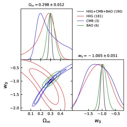
$\begin{array}{c}\end{array}$

(a) HIIG+CMB+