DiagSet: a dataset for prostate cancer histopathological image classification

Abstract

Cancer diseases constitute one of the most significant societal challenges. In this paper we introduce a novel histopathological dataset for prostate cancer detection. The proposed dataset, consisting of over 2.6 million tissue patches extracted from 430 fully annotated scans, 4675 scans with assigned binary diagnosis, and 46 scans with diagnosis given independently by a group of histopathologists, can be found at https://ai-econsilio.diag.pl. Furthermore, we propose a machine learning framework for detection of cancerous tissue regions and prediction of scan-level diagnosis, utilizing thresholding and statistical analysis to abstain from the decision in uncertain cases. During the experimental evaluation we identify several factors negatively affecting the performance of considered models, such as presence of label noise, data imbalance, and quantity of data, that can serve as a basis for further research. The proposed approach, composed of ensembles of deep neural networks operating on the histopathological scans at different scales, achieves 94.6% accuracy in patch-level recognition, and is compared in a scan-level diagnosis with 9 human histopathologists.

1 Introduction

In highly developed countries, prostate cancer is the second most common cause of death in men after lung cancer. Prostate cancer is one of the most common malignant neoplasms in men. The choice of treatment method depends mainly on the clinical stage and malignancy of the cancer defined according to the Gleason scale (Albelda, 1993; Konig et al., 2004; Gleason, 1966) and the ISUP classification 2014 by the ISUP grade group (Epstein et al., 2016). Such diagnoses are made by histopathologists. However, the number of professional doctors is very limited and continues to decline compared to social needs. There are many reasons for this, such as long training time or the increasing number of diagnoses required in a short time. A solution to this situation is the use of modern classification systems based on deep learning technologies. Nevertheless, the construction of such systems requires participation of the professional histopathologists, for example in the process of preparing and annotating samples of healthy and cancer affected tissues.

In this paper, we present and share a new set of histopathological data, called DiagSet, containing the annotated regions of prostate tissues in the whole slide imaging (WSI) scans characterized by different Gleason degrees. We also present the structure and the results of operation of the individual as well as an ensemble of the convolutional neural networks appropriately trained for the classification of histopathological images of the prostate WSI. First, AlexNet, VGG16, VGG19, ResNet50 and Inception V3 networks were trained and their performance analysed. Second, these networks were used again but this time cooperating in an ensemble, wherein each classifier was trained with images of a different magnification factor, after which the individual probabilities returned by each network were combined to produce the final result. Then few rules has been developed and used to produce the binary diagnosis. For this purpose a discrimination rule has been devised, underpinned with the rules operating with the parametric and non-parametric statistical hypothesis testing methods for further response verification. The best binary classification ratio obtained with the ensemble architecture is 94.58%. An experiment was then conducted in which nine volunteer professional histopathology doctors participated, making individual diagnosis on a set of forty six anonymous WSI scans. Then the correlations of their responses were computed, as well as correlations of their responses in respect to the machine given diagnosis by the proposed method. The obtained measurements showed that, except one WSI scan, examination correlation of the machine response is within the correlation range obtained between the participating doctors.

The main contributions of this paper can be summarized as follows:

• Introduction of a novel prostate cancer histopathological image dataset, consisting of 430 fully annotated scans, 4675 scans with assigned binary diagnosis, and 46 scans with diagnosis given independently by a group of 9 histopathologists.

• Identification and experimental evaluation of several factors negatively influencing the performance of machine learning models trained on the proposed dataset, with the aim of outlining future research directions.

• Proposal of a machine learning framework for detection of cancerous tissue regions and prediction of scan-level diagnosis, utilizing thresholding and statistical analysis to abstain from the decision in uncertain cases.

• Experimental comparison of the proposed framework with a group of human histopathologists.

The rest of the paper is organized as follows. An overview of related works is presented in Section 2. In Section 3 the properties and structure of the DiagSet are described. Our classification methodology, based on the deep neural architectures, is presented in Section 4. After that, in Section 5 the statistical hypothesis testing methods, used for verification of the diagnosis based on the probability distributions of the image patches, are described. In Section 6 the results are presented and discussed. The paper ends with conclusions in Section 7.

2 Related work

The main deep neural models applied in computational histopathology fall into one of the following groups:

• Supervised learning.

• Weekly supervised learning.

• Unsupervised learning.

• Transfer learning.

The above schemes can be realized by different neural architectures, such as various types of convolutional (CNN) or recurrent neural networks (RNN), as well as autoencoders (AE) and generative adversarial networks (GAN), or a more complex system composed of these, respectively. Also, different histopathological features can be applied, such as entire cells, nuclei, glands, tissue texture or a combination of these (Spanhol et al., 2016)(Wan et al., 2017)(Pan et al., 2017). Hence, the potential space of solutions is ample. Recent overviews of deep neural models in cancer diagnosis histopathology are presented e.g. in the papers by Chetan et al. (Srinidhi et al., 2019), Litjens et al. (Litjens et al., 2017), as well as Janowczyk & Madabhushi (Janowczyk and Madabhushi, 2016). It was shown that the modern data-oriented approaches with deep neural networks outperform the previously developed methods based on expert proposed hand crafted features and models. The patch-based cancer classification of the WSI scans was employed by many researchers; for example Litjens et al. proposed the CNN for the prostate and breast cancer diagnosis from the H&E scans (Litjens et al., 2016), while Vandenberghe et al. for the breast cancer (Vandenberghe et al., 2017). In all such systems the vital part is preparation of the training datasets with proper patch labelling. In the case of the prostate cancer, which we are concerned mostly in this paper, a degree or the prostatic carcinoma is described with the well established Gleason scale (Epstein et al., 2005). The name of the scale comes from the name of an American pathologist - Dr. Donald Gleason, working at the Minneapolis Veterans Affairs Hospital. His publication appeared in 1966 (Gleason, 1966). Therefore in the case of the supervised classification of the prostate cancer the most natural labeling is just based on the Gleason scores. This strategy has been undertaken by many researchers and also in our research. For example Bulten et al. propose grading and prostate cancer detection based on the UNet segmentation with respect to the growth of the Gleason patterns which are followed by the subsequent cancer grading (Bulten et al., 2020). Campanella et al. also proposed a system for prostate cancer detection in WSI (Campanella et al., 2018). Arvaniti et al. discuss the problem of the deep multiple instance learning for classification and localization of the prostate cancer (Arvaniti et al., 2018). On the other hand, classification of the prostate tissues into tumor vs. non-tumor based on convolutional adversarial autoencoders was proposed by Bulten and Litjens (Bulten and Litjens, 2018). For this the WSI dataset from the Radboud University Medical Center has been used, which scans are hematoxylin and eosin (H&E) stained. Interestingly, Ren et al. proposed unsupervised training of the Siamese neural network for the prostate WSI patch based classification (Ren et al., 2018).

A research on development and validation of a deep learning algorithm for improving Gleason scoring of prostate cancer has been performed by Nagpal et al. (Nagpal et al., 2019). Because the Gleason scoring among the pathologists is highly subjective and suffers from inter and intra-observer variability, with the discordance ratio reported to be in the range 30%-50%, Nagpal et al. in investigate performance of the deep neural network, for providing an automatic and reproducible method for feature extraction.

Nir et al. conducted an extensive research into the automatic grading of prostate cancer in digitized histopathology images (Nir et al., 2018). Extensive experiments with various classifiers, such as linear discriminant analysis (LDA), support vector machines (SVM), logistic regression (LR), and random forests (RF), operating with a broad set of hand crafted features, as well as deep neural networks, were carried on. Interestingly, the best results in terms of accuracy and overall agreement were obtained by LR with the hand crafted features, whereas the worst were observed with SVM. Also, interestingly DNN performed well, but not the best, due to insufficient number of training data and probably not sufficiently deep architecture, as concluded by the authors.

3 Dataset

For preparation of the dataset randomly selected microscopic specimens of biopsy specimens, i.e. sections from prostate tumors of patients diagnosed with adenocarcinoma of the prostate, were subjected to research and experiments. Microscopic slides were made in the classical formalin-paraffin technique in the histopathology laboratory. Prostate biopsies, after fixation in 10% formalin (10% buffered formalin, 4% formaldehyde content, manufacturer: ALPINUS CHEMIA Ska z o.o.), were embedded in paraffin blocks. Subsequently, in the course of cutting (MICROM HM355S microtome) preparations with a thickness of 5-7 micrometers were obtained, which were stained with hematoxylin and eosin (H&E). The diagnostic assessment was performed by doctors pathomorphologists employed at Diagnostyka Consilio. According to the current procedure, each preparation was assessed independently by two pathologists.

The basis for the analysis was the binding classification Gleason system (Gleason, 1966). The classic Gleason system includes five grades (scale from 1 to 5), where the subsequent grades indicate the higher malignancy of the assessed cancer zone. The assessment result (diagnosis) of the test is reported by the pathologist as the sum of the points (Gleason score; GS) allocated to the most diverse zones within the cancer area in the tissue/specimen tested. First, the score for the dominant feature in the examined tissue is given, and then the score for the second largest feature. The final score / diagnosis is given as the sum of the points (on a scale of 1 to 5), which means that the assigned Gleason score can have a score of 2 (1 + 1) up to 10 (5 + 5).

On this basis, a simple cancer grading system in the peraparate was defined: Gleason sum 2-4 - low grade I tumor malignancy / aggression, Gleason sum 5-7 - moderate II degree of tumor aggression, Gleason sum 8-10 - very high III degree of tumor aggression.

In 2014, new guidelines were published, developed within the international organization ISUP (Epstein et al., 2016). ISUP grade group - introduced five mischief groups that combine different grades of Glaeason score according to the scheme: group 1 according to ISUP is Gleason score 3 + 3 = 6 group 2 is 3 + 4 = 7 group 3 is 4 + 3 = 7 group 4 are all GS combinations giving a score of 8 group 5 are all GS combinations giving a score of 9. ISUP groups omit Gleason Grades 1 and 2.

In our research the following assumptions were undertaken:

• Three pathologists evaluating scans.

• Scans of original and archival microscopic slides.

• Unknown primary diagnosis.

• Assessment consisted in outlining the fields on a computer scan according to the following encoding (labels):

  • R1, R2, R3, R4, R5 - Gleason adenocarcinoma fields,

  • T - background field (any area outside the cancer tissue),

  • A - artifacts.

A total of over five thousand scans were included in the pathomorphological assessment. The dataset can be be found at https://ai-econsilio.diag.pl.

3.1 Data acquisition

All scans where acquired with the Hamamatsu C12000-22 digital slide scanner. The scanner uses time delay integration (TDI) scanning method. The magnification (objective lens) was $40\times$. All slides where scanned in one $z$-stack layer with dynamic pre-focus and pre-focus map. Before scanning slides where inspected for overhanging labels and traces of the felt tip pen then where wiped with soft cloth to remove loose debris, water spots, or fingerprints from the upper and lower surface. For difficult slides alcohol solution where used. Often when tissue of prostate needle biopsy was narrower than 0.5 mm it was omitted in the scanning area. It happened once in every 300 cases of the prostate needle biopsy slides. Sometimes, if parts of the slides where blurry it was caused by the folded or rugged surface of a tissue.

The slides where scanned in unattended mode using the feeder for 320 slides. The area of scan, as well as the focal points, where set automatically. The median scan time per slide at $40\times$ equivalent resolution (0.25 µm/pixel) was 3 minutes. The average file size was 1.2 gigabytes (GB). To recognize the tissue type we use barcode recognition and then query to external slide database. All images where stored on the disk array in the NDP format. We used the Slide distribution and management software NDP.server3. The NDP.Server software API was used to access the slide images, annotations, detailed slide data (magnification, scan info, barcode label, etc.) The JPG slide images where acquired by means of the NDP tiles server API.

3.2 DiagSet-A

First part of the proposed dataset, DiagSet-A, consists of small image patches extracted from the underlying WSI scans, with labels assigned based on the annotation made by human histopathologists. Patches with a size of $256\times 256$ were extracted from the scans with a stride of 128, at 4 different magnification levels: $40\times$, $20\times$, $10\times$ and $5\times$. Each patch was assigned a single label out of 9 possible classes: scan background (BG), tissue background (T), normal, healthy tissue (N), acquisition artifact (A), or one of the 1-5 Gleason grades (R1-R5). Samples for each class and magnification level are presented in Figure 1.

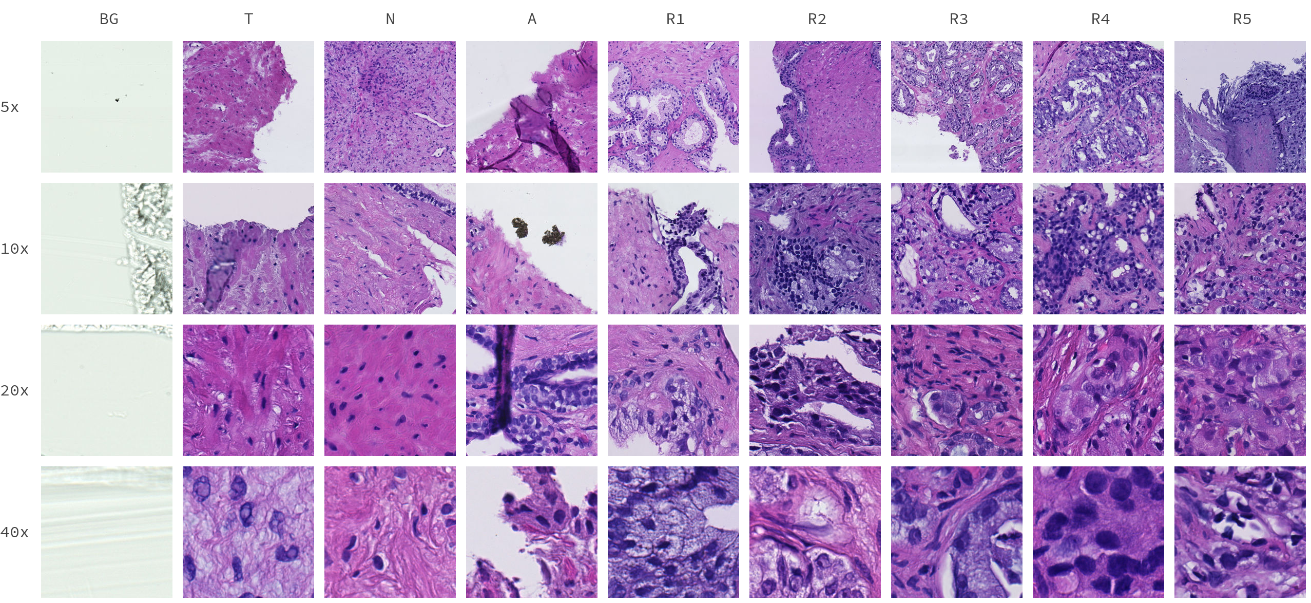
Figure 1: Randomly selected samples of image patches from DiagSet-A, extracted at different magnifications (rows) and containing different classes of tissue (columns).

During the labeling process a histopathologist annotated larger WSI regions as belonging to one of the defined classes. Due to the nature of the labeling process some patches can be covered by annotations only partially, or contain multiple overlapping annotations. To translate these annotations to labels on the patch level the following procedure was used: on the highest magnification level, that is $40\times$, a label was assigned if and only if only a single class annotation with overlap ratio equal to or higher than 0.75 was present. In this case that annotation label was assigned as a class associated with a given patch. If either none of the classes overlapped the patch at a specified ratio, or multiple contradictory labels were present, the patch was not assigned any class. Secondly, on lower magnification levels, that is $20\times$, $10\times$, or $5\times$, a patch was first divided into smaller $40\times$ patches (4 in case of $20\times$ magnification, 16 in case of $10\times$, and 64 in case of $5\times$). Each $40\times$-level patch was assigned a label according to the previously described procedure. Finally, the most severe of the $40\times$-level labels were assigned as a final label for the lower magnification patch. For instance, if given $20\times$-level patch could be divided into one $40\times$-level patch with a label N, two $40\times$-level patches with R3 label, and one $40\times$-level patch with R4 label, the R4 label would be assigned to the $20\times$-level patch.

Due to the length of the annotation process, as well as the time required to train described machine learning models on a large quantities of data, and for the sake of the experimental study described in later part of this paper, DiagSet-A was divided into two parts. First, DiagSet-A.1, consists of 238 WSI scans annotated by the histopathologists. DiagSet-A.1 was used in the majority of the preliminary experiments described in Section 6. Secondly, DiagSet-A.2, which compared to the DiagSet-A.1 consists of 190 additional training scans, as well as a single additional validation and test scan. Importantly, DiagSet-A.2 also introduced additional class, BG, which was not originally present in the dataset. DiagSet-A.2 was used during the final evaluation of the proposed approach, and can be treated as a final version of the dataset. Detailed number of scans and patches extracted for both version of the dataset are presented in Table 2, whereas their class distribution is presented in Table 1.

Table 1: Class distribution of the DiagSet-A.1 (initial dataset, used in the preliminary experiments) and DiagSet-A.2 (final dataset).

Version	BG	T	N	A	R1	R2	R3	R4	R5
DiagSet-A.1	0.0%	24.8%	44.6%	2.0%	0.6%	0.8%	6.6%	17.1%	3.4%
DiagSet-A.2	6.6%	23.8%	35.3%	8.3%	0.7%	0.7%	6.1%	15.4%	3.0%

Table 2: Detailed number of scans and extracted patches in the specific data partitions.

Version	Partition	# of scans	Magnification	# of patches
DiagSet-A.1	train	156	$40\times$	850,860
			$20\times$	273,321
			$10\times$	90,746
			$5\times$	32,981
	validation	41	$40\times$	215,071
			$20\times$	70,013
			$10\times$	23,189
			$5\times$	8,374
	test	41	$40\times$	267,691
			$20\times$	86,888
			$10\times$	28,945
			$5\times$	10,507
		238		1,958,586
DiagSet-A.2	train	346	$40\times$	1,250,661
			$20\times$	398,201
			$10\times$	132,882
			$5\times$	48,782
	validation	42	$40\times$	245,441
			$20\times$	77,889
			$10\times$	25,294
			$5\times$	8,977
	test	42	$40\times$	284,032
			$20\times$	91,125
			$10\times$	30,086
			$5\times$	10,836
		430		2,604,206

3.3 DiagSet-B

Second part of the presented dataset, DiagSet-B, consists of 4675 WSI scans with a singly binary diagnosis denoting either a presence of cancerous tissue on the scan (C) or lack thereof (NC), with 2090 scans belonging to the C class, and 2585 belonging to the NC class, respectively. These scans were extracted from the archive of patient treatments, with labels assigned based on the text of diagnosis given by a human histopathologist. Label assignment based on the text of diagnosis was conducted manually. It should be noted that compared to the DiagSet-A, which was annotated solely based on the underlying WSI scan, the diagnoses used in DiagSet-B were given in a normal course of patient treatment and were potentially based on additional medical data, such as the results of the immunohistochemistry examination (IHC).

3.4 DiagSet-C

Third part of the presented dataset, DiagSet-C, consists of 46 WSI scans with a global diagnosis given independently by a larger number of 9 human histopathologists. Unlike DiagSet-B, while labeling scans in DiagSet-C, histopathologists were asked to assign each scan one of the three possible labels: containing cancerous tissue (C), not containing cancerous tissue (NC), or uncertain and requiring further medical examination (IHC). Compared to DiagSet-B, including IHC in the set of possible labels more closely resembles actual process of the histopathological diagnosis, in which WSI scan is often insufficient to make a decision. Furthermore, aggregating the diagnoses of several medical practitioners allows us to evaluate the agreement within the population of histopathologists, as will be discussed.

3.5 SegSet

Finally, in the process of constructing a production model another dataset named SegSet was created. SegSet consists of 30 downsampled WSI scans containing prostate, breast and colon cancer tissue together with binary segmentation mask denoting the presence of valid tissue. A sample image from SegSet, together with the associated mask, is presented in Figure 2. In the conducted experiments SegSet was used to train a preprocessing segmentation model that, on a lower magnification, excluded scan background (BG) and data acquisition artifacts, in order to reduce the computational overhead of further patch-level classification. The preprocessing step is further discussed in Section 4.

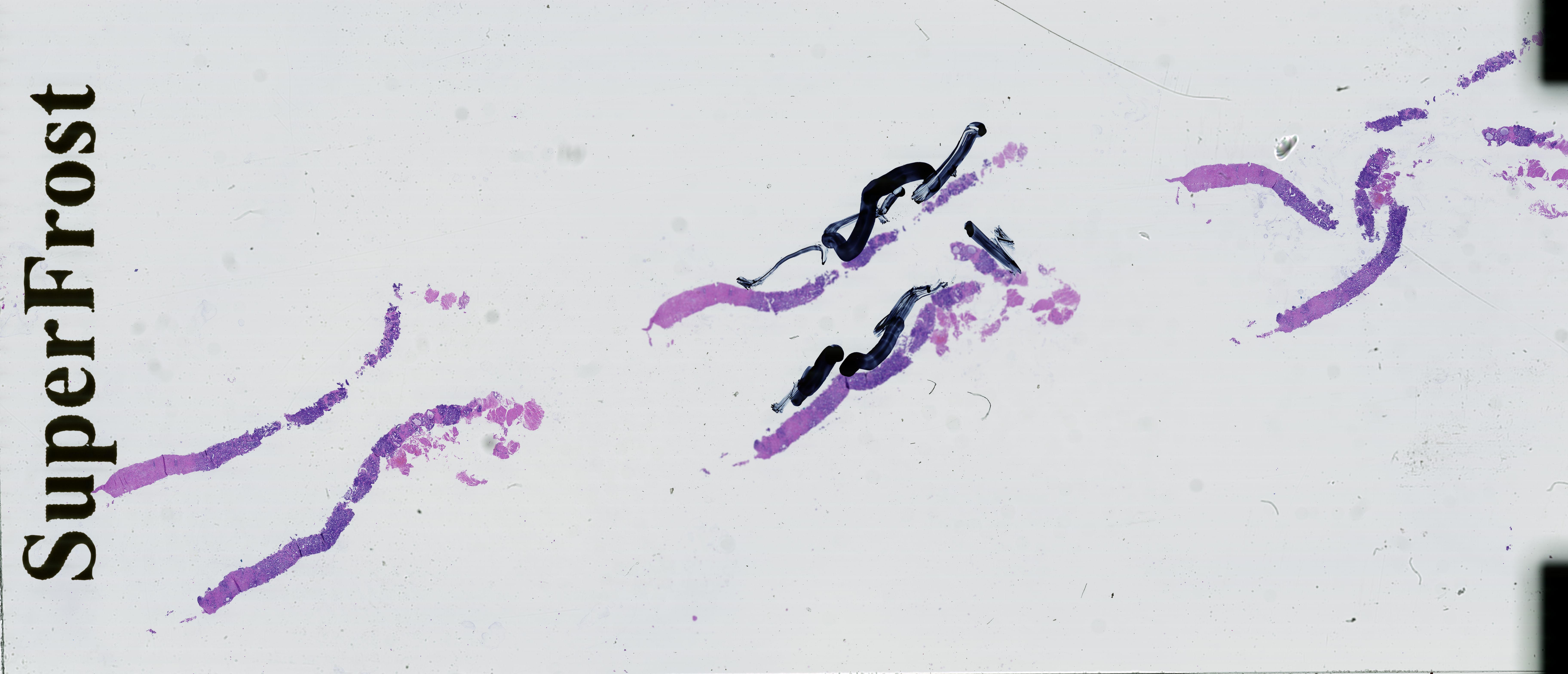
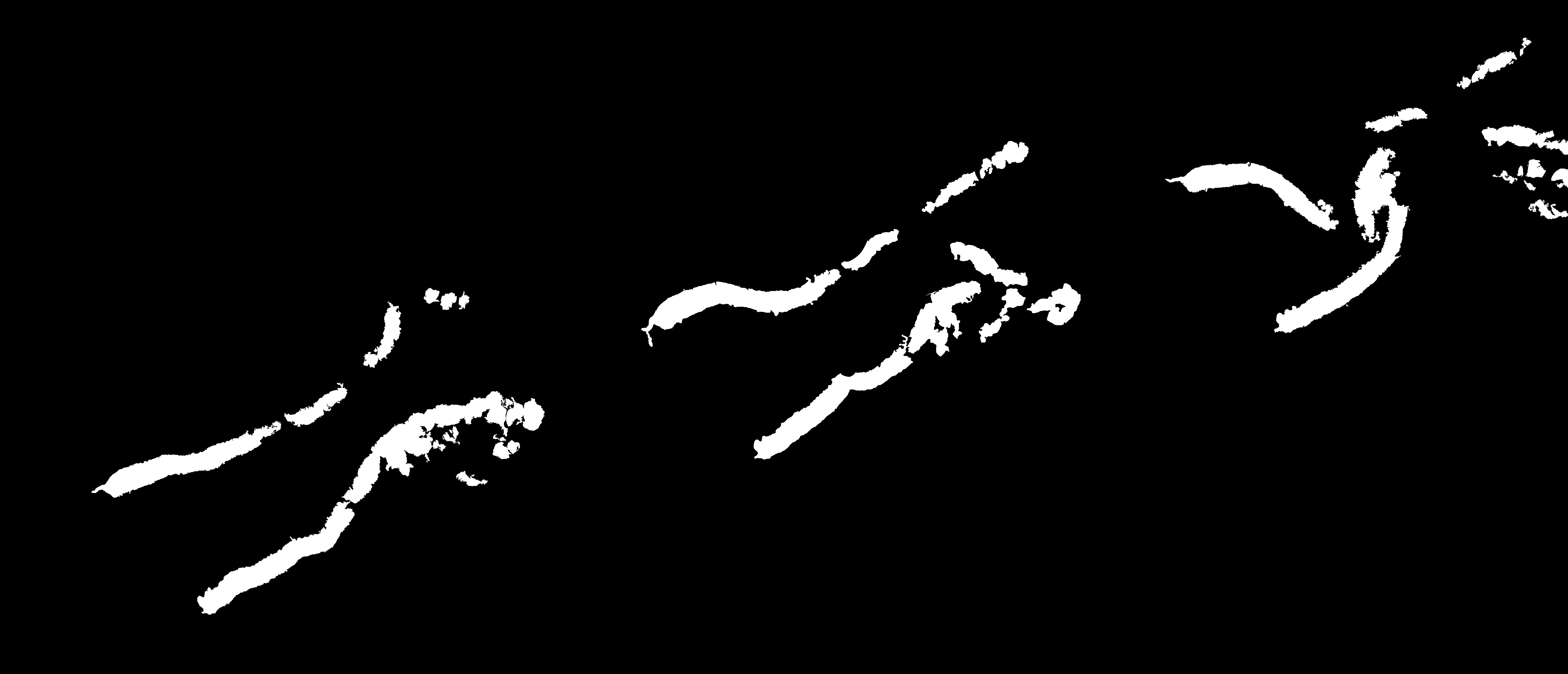
Figure 2: Randomly selected sample of an image from SegSet dataset (left) and corresponding binary mask, denoting the presence of a valid tissue (right). Note the presence of artifacts on the underlying image, such as slide brand name and markings made on the slide around selected tissue fragments.

4 Methodology

When dealing with histopathological image recognition models, operating on WSI scans, two main tasks can be distinguished. First of all, recognition of scan regions containing cancerous tissue, either on a binary cancerous/non-cancerous level, or a more fine-grained recognition of cancer types, such as the Gleason grades. Secondly, prediction of an overall diagnosis for the whole scan, possibly based on the previously recognized cancerous regions. In this paper we consider a methodology dealing with both of these steps, and relying on fragmentation of whole WSI scan into small image patches, that can be then treated as individual images in the image classification task. The proposed methodology consists of the following steps:

Valid tissue segmentation: in the initial step of the proposed machine learning pipeline we conducted a preprocessing in form of valid tissue segmentation, with the aim of reducing the computational overhead associated with classification of a large number of individual patches. To these end we extract an image of a whole WSI scan downsampled with the factor of 8 and, using a fully convolutional neural network, perform a supervised image segmentation, with the goal of predicting a binary mask containing an information on whether any given pixel contains valid tissue (that is, not scan background or acquisition artifact, as discussed in the description of SegSet dataset). Since typically a majority of WSI scan consists of the scan background, this operation can have a substantial impact on the computational overhead. In this step we used a variant of fully-convolutional VDSR network (Kim et al., 2016), which consisted of 10 convolutional layers with 64 $3\times 3$ filters each, trained on $21\times 21$ image patches for 600 epochs using Adam optimizer with learning rate equal to 0.0001 and weight decay equal to 0.0001.

Single-model patch recognition: in the second step of the proposed pipeline we performed image classification using small scan patches, extracted from the original WSI scan. The goal of this step was to produce probability maps for a given scan, indicating the likelihood that a tissue at a given spatial position belongs to one of the predefined classes. To this end we divided the scan into $224\times 224$ patches and independently classified every one of them using a previously trained convolutional neural network. Importantly, we conducted this procedure for a number of neural architectures, as well as several magnification factors, to compute a collection of probability maps for each of the model/magnification combinations.

It is worth noting that such classification of small WSI patches is equivalent to rough image segmentation, with a number of notable approaches for this problem already existing, such as U-Net networks. Nevertheless, in this paper we decided to formulate the problem as a patch classification task due to two reasons: 1) we suspected that data imbalance can pose a significant challenge given the dataset characteristic; mainly the class distribution, and a larger body of methods for dealing with class imbalance within the classification framework already exists, and 2) we decided that prediction granularity with sufficiently small patches, such as $224\times 224$, will be sufficient for our purposes.

Throughout the conducted experimental study we considered several notable architectures of the convolutional neural networks proposed in the recent years: AlexNet (Krizhevsky et al., 2012), VGG16 and VGG19 (Simonyan and Zisserman, 2014), ResNet50 (He et al., 2016) and InceptionV3 (Szegedy et al., 2016). All of the models were trained for 50 epochs using the SGD optimizer with initial learning rate equal to 0.0001, decayed after each 20 epochs with a rate of 0.1, and batch size equal to 32. All of the models were regularized using weight decay equal to 0.0005. Additionally, AlexNet and both VGG models used dropout equal to 0.5. To augment the data, during training we cropped random $224\times 224$ patches from the original $256\times 256$ images, and afterwards applied random horizontal flip and rotation by a random multiple of a 90 degree angle. During the evaluation we instead used a central cropping to obtain the same patch size. In both cases input images were preprocessed by subtracting the ImageNet (Deng et al., 2009) image mean, that is a tuple (123.680, 116.779, 103.939). Unless otherwise specified, the weights of all of the models were transferred from a model trained on the ImageNet dataset.

Model ensembling: in the third step of the proposed pipeline we combined probability maps generated by individual models using ensembling. Specifically, several probability maps were combined by averaging the probabilities returned by the individual models. While using ensembling to improve performance is a common practice, in the histopathological image recognition task in addition to combining the predictions made by different architectures of neural networks we also propose combining models trained on different tissue magnifications. We take advantage of the fact that, while the model trained on a higher magnification will have to make predictions for a larger number of patches to encompass the same region as the model trained on a lower magnification, spatially they correspond to the same scan region. As a result, we simply rescale probability maps generated by higher magnification models to a common dimensionality, after which we can once again combine their predictions by map averaging.

Scan-level diagnosis: finally, to translate the patch-level probability maps generated in previous steps into a single scan-level diagnosis we considered an approach of thresholding the ratio of scans patches that were classified as cancerous to the overall number of valid tissue patches. Specifically, we used a simple decision-making rule based on two parameters, lower threshold $T_{L}$, and upper threshold $T_{U}$, that based on the percentage of valid tissue patches (that is, all patches excluding BG class and scan background excluded during the initial segmentation step) of a given scan $p_{c}$, gave a diagnosis ’non-cancerous’ if $p_{c}\leq T_{L}$, ’cancerous’ if $p_{c}\geq T_{U}$, and abstained from making the decision if $T_{L}<p_{c}<T_{U}$. Such decision rule can be interpreted as a simple abstaining classification algorithm, which optimizes a multi-objective criterion: on the one hand we wish to achieve as high diagnosis accuracy as possible, while on the other we wish to abstain from giving the diagnosis in the least possible number of cases. Both criteria are clearly opposing, since by reducing the width of the range in which we abstain from making the prediction we decrease the chance of error, and vice versa. It is also not clear what cost should be assigned to an incorrect diagnosis and to abstaining from making the decision, making the problem ambiguous. Because of that, instead of presenting a single result of a chosen model, we examined the trade-off associated with choosing different values of $T_{L}$ and $T_{U}$. However, this decision-making rule, called DCNN, has been backed up with the statistical hypothesis testing framework described in the next section.

5 Statistical analysis of the patch distributions

Statistical hypothesis testing framework. In the process of the whole slide classification the neural networks output probabilities for each of the processed slide patches. Low probability values correspond to the patches containing healthy tissues, whereas cancer affected ones are attributed higher probabilities. In this scheme only two cases are considered: the healthy (normal, no-cancer) NC and the cancer C samples, respectively, as annotated by the histopathology experts. The low probability patches are common to the two populations, whereas high probability patches can be encountered only in the C population. This feature gives rise to the statistical hypothesis testing framework. Namely, we wish to construct a statistical test that will be able to provide the answer if a given statistics of an unknown WSI follows the statistics of the NC or C populations. The first step is to analyze types of the two distributions, whose histograms are shown in Fig. 11.

The C histogram reveals high tails which correspond to the high concentration of the patches not affected by the cancer changes, as well as also visible but smaller right tail corresponding to the highly affected ones. As expected, the NC histogram contains high left tail corresponding to the patches whose cancer probabilities are close to zero.

In the investigated method we wish to answer the question if the set of patch probabilities from the unknown WSI follows the population of the C or NC patches, cumulatively obtained from many human annotated WSI examinations performed by the pathologists. Hence, we come with the two-sample testing problem. More precisely, we will investigate two null hypothesis: if the $X_{1}$ sample comes from the $X_{C}$ population or if $X_{1}$ comes from the $X_{NC}$ population. The statistically satisfactory tests should be strong enough to either reject the two hypothesis or accept the only one. However, the statistical test have also to be chosen in accordance with its assumptions. For example, the well established group of the parametric t-tests assume normal distributions (Sheskin, 2007). On the other hand, the nonparametric tests, such as the Wilcoxon-Mann-Whitney (WMW) or the permutation tests, do not superimpose any special assumptions upon the data distributions but in many cases they are not strong enough to provide meaningful answers. Therefore, in our research we decided to test performance with each of the aforementioned two-sample tests. Below we provide a short characteristic of each of them, as well as we state the precise assumptions of their usage in the cancer diagnosis based on the set of patch responses from the deep neural network. Each different hypothesis test with its chosen statistical decision rule is called a statistical perspective. Finally, results of each tested statistical perspective are presented and discussed.

• The Welch parametric t-test

For the samples of different variances, the Welch’s modification of the t-test should be used. Under the Behrens-Fisher statistical perspective, for the two samples

$${X_{1}=\{x_{11},x_{12},...,x_{1N_{1}}\},X_{2}=\{x_{21},x_{22},...,x_{2N_{2}}\}}$$ (1)

each containing $N_{1}$ and $N_{2}$ values, respectively, it reads as follows

$$T_{BF}(X_{1},X_{2})=\frac{\bar{X}_{1}-\bar{X}_{2}}{\sqrt{(}s_{1}^{2}/N_{1}+s_{2}^{2}/N_{2})}$$ (2)

where $\bar{X}_{i}$ denotes a mean and $s_{i}^{2}$ a standard deviation of an i-th sample, respectively. Welch’s decision rule (a critical function) is computed based on the the predetermined significance level $\alpha$, and the q-th quantile of the t-distribution with $\eta$ degrees of freedom. The latter is given by the Welch–Satterthwaite equation, as follows

$$\eta=\frac{\left(\frac{s_{1}^{2}}{N_{1}}+\frac{s_{2}^{2}}{N_{2}}\right)^{2}}{\frac{s_{1}^{4}}{N_{1}^{2}(N_{1}-1)}+\frac{s_{2}^{4}}{N_{2}^{2}(N_{2}-1)}}$$ (3)

Some further properties of the Welch test are provided in the work by Derrick et al. (Derrick and White, 2016). They showed that the Welch test is more robust to the type I errors in respect to the t-test. An important issue is the underlying assumption of the data normality which at the first sight excludes a direct usage of this type of test, also for the cancer detection problem analyzed in our work. A first attempt to remedy this is to apply a transformation which converts the underlying distribution into the normal one. This idea is based on the Central Limit Theorem, which shows that if independent random samples of a given size are repetitively taken from the underlying population, then the distribution of the samples’ means approaches the normal distribution, assuming sufficiently large samples and the large number of drawings. As indicated by Choi (Choi, 2016), many real life distributions are highly non-normal and even their transformations by the sample means drawing will not approach a clearly normal distribution. This would suggest rather nonparametric tests, such as the WMW. However, many researchers advocate using t-tests, rather than the nonparametric ones, even for not normally distributed data. For example Fagerland (Fagerland, 2012) showed on the gamma and lognormal distribution poor behavior of the WMW test, contrasted with the t-test. The finding is that the WMW test is most suitable for the ordinal data and smaller studies. However, for the larger studies, when the purpose is to compare the means the t-test is recommended as being robust even for the highly skewed distributions. Based on the above analysis we decided to use the Welch version of the t-tests in our experiemnts and compare their results with the WMW and permutation based nonparametric approaches.

• The nonparametric Wilcoxon-Mann-Whitney (WMW) rank-sum test

The WMW is a nonparametric test with the null hypothesis reading that it is equally likely that a random sample $X_{1}$, selected from one population, is less than (or greater than) a random sample $X_{2}$, selected from the second population. The WMW test is two-sample rank sum test. In our experiments the nominal patch probabilities of the $X_{1}$ and $X_{2}$ samples can be directly used as the rank values, i.e. each observed probabilities can be ordered. Under the null hypothesis $H_{0}$ the distribution of the two tested populations are equal, whereas $H_{1}$ is the alternative, i.e. that these distributions are not equal. Computation of the WMW test is based on computation of the $U$ statistics whose distribution under the $H_{0}$ is assumed to be known. The procedure of calculating the $U$ statistics from the two samples $X_{1}$ and $X_{2}$ is as follows:

1. The two sets $X_{1}$ and $X_{2}$ defined in Eq. (1) are joined into one set

   $${Y=\{X_{1},X_{2}\}}$$ (4)

2. The ranks $R_{ij}$ of each $x_{ij}$ in the above set $Y$, i.e. their relative positions, are calculated.

3. The $U_{1}$ and $U_{2}$ values are computed as follows:

   $${U_{1}=N_{1}N_{2}+\frac{N_{1}(N_{1}+1)}{2}-\sum_{n=1}^{N_{1}}R_{1n}}$$ (5)

   and

   $${U_{2}=N_{1}N_{2}-U_{1}}$$ (6)

4. Under the assumption that the null hypothesis is true, the following statistics

   $${Z_{WMW}(X_{1},X_{2})=\frac{U-E(U\rvert H_{0})}{\sqrt{(Var(U\rvert H_{0})}}}$$ (7)

   approximates the normal distribution, where for the two-tailed test considered in our experiments,

   $${U=min\{U_{1},U_{2}\}}$$ (8)

   $${E(U\rvert H_{0})=\frac{N_{1}N_{2}}{2}}$$ (9)

   and

   $${Var(U\rvert H_{0})=\frac{N_{1}N_{2}(N_{1}+N_{2}+1)}{12}}$$ (10)

   (assuming no tie groups are present).

Based on the above procedure, the WMW decision rule follows the q-th quantile of the normal distribution under the $\alpha$ significance level.

We should also note a difference in the statistical perspective between the WMW and the Welch tests, since the former is concentrated around giving an answer how likely is the $X_{1}$ sample less (or greater) than a random sample $X_{2}$, whereas the latter is concerned about providing an answer on equality of the means of $X_{1}$ and $X_{2}$. Although, these two perspectives may have some common points – for example if $X_{1}$ is much less than the $X_{2}$ then probably their means are also different – they are different perspectives. Therefore, for the third the nonparametric permutation test is chosen whose perspective is equality of the means (or, in general case, other chosen statistics). As shown by Fay and Proschan (Fay and Proschan, 2010), the WMW test can be used for the statistical perspectives concerning differences in means, as well as differences of the distributions. They also argue that, although converting the numerical to the rank values lowers power of the WMW tests, in the cases of extremely heavy tailed or skewed distributions WMW can get better power that the t-test. However, for less heavily tailed distributions the t-test is recommended. Moreover, when coming to the choice between the t-test (Welch) and the WMW, Fay and Proschan recommend not to base on the normality test, since under general condition the t-test decision rules are asymptotical even when the normality assumption is rejected. This stays in concordance with the finding provided by Fagerland (Fagerland, 2012). Also Fagerland and Sandvik showed poor performance of the WMW test for comparing means or medians of two populations which deviate from the same shape or equal scales (Fagerland and Sandvik, 2009). For the mean comparison of the equal size samples the parametric Welch test is superior to the rank based tets. In the result, all these researches recommend choice of the t-test family over the nonparametric WMW tests, even for testing of highly not normal distributions and especially if the difference in the means is investigated. On the other hand, WMW may be asymptotically more powerful for data contaminated with gross errors, since the ranks are more robust to outliers than the numerical values in the t-test (Fay and Proschan, 2010). Because of these, in our method all the tests are performed on the samples of equal size, with the Welch test being the preferable one.

• The nonparametric permutation test

The permutation test can be used to compare various statistics of the two samples without any assumption on the underlying distribution. Hence, it can be used to test if the distributions of the two samples are identical or if their means are identical, and so on. Foundations of the permutation methods were laid by Fisher in 1935. It is based on the assumption that if the two samples really come from the same (usually unknown) distribution, then the statistics computed on these samples, as well as on their permutations, should be statistically the same over a sufficiently large number of permutations (Ernst, 2004). First, let us define the observable test statistics between the general samples $U$ and $V$, as follows:

$${s(U,V)=|\bar{U}-\bar{V}|}$$ (11)

where $\bar{U}$ and $\bar{V}$ denote the mean values of $U$ and $V$, respectively. Now, for the samples $X_{1}$ and $X_{2}$, defined in Eq. (1), the permutation test is computed as follows.

1. From Eq. (11) compute the reference test statistics of the initial samples $X_{1}$ and $X_{2}$:

   $${s_{0}(X_{1},X_{2})=s(X_{1},X_{2})}$$ (12)

2. Join the samples $X_{1}$ and $X_{2}$ into $Y$, as in Eq. (4).

3. For each i-th permutation $Y_{i}$ of $Y$ split it with the ratio $N_{1}:N_{2}$ into two new samples $X_{1i}=\{y_{i1},...,y_{i{N_{1}}}\}$ and $X_{2i}\{y_{i{N_{1+1}}},...,y_{i_{N_{2}}}\}$.

   Compute the one-sided p Monte Carlo value for a test of rejecting the null hypothesis based on a large number of computed values of the statistics $s_{i}$, as follows

   $${p=P(s>s_{0}\rvert H_{0})=\frac{1+\sum_{i=1}^{M}I(s_{i}>s_{0})}{M+1}}$$ (13)

   where

   $${s_{i}=s(X_{1i},X_{2i})}$$ (14)

   and

   $${M\leq\binom{N}{N_{1}}=\binom{N_{1}+N_{2}}{N_{1}}=\frac{(N_{1}+N_{2})!}{N_{1}!N_{2}!}}$$ (15)

   denotes the number of randomly sampled permutations, and I is the indicator function.

The decision rule for the permutation test is p>$\alpha,$ where the latter denotes the significance level. The drawback of the permutation test is the long computation time. That is, in practice it is almost never possible to verify all of the data permutations, while even their subset – which if not large enough may jeopardize the statistical property of this test – usually requires much longer computations than the Welch or WMW tests.

Classification based on statistical hypothesis. The above described three statistical tests are separately used to answer a question if a given population of probabilities, corresponding to the patches of a test WSI, follows distribution of the grand population of patches of all WSI classified by the histopathologists as belonging either to the C or NC classes, respectively. For this purpose the following algorithm is proposed.

1. Input: A sample $X$ from the test WSI, collected populations of $X_{C}$ and $X_{NC}$ patch probabilities; $n$ the number of iterations (Parameters defined in Table 13)

2. Output: A label $D\in\{C,NC,IHS\}$ of the sample $X$

3. $i=0$

4. while $i<n$

5. From $X_{C}$, $X_{NC}$ and $X$ draw random samples

   $X_{Cs}$, $X_{NCs}$, and $X_{s}$ of size $s$ each

6. Perform and store results of the statistical tests

   $H(X_{Cs},X_{s})$ and $H(X_{NCs},X_{s})$

7. $i=i+1$

8. if $X_{CH}$ has passed at least by the factor $r$, then $D_{C}$ is true

9. if $X_{NC}$ H has passed at least by the factor $r$, then $D_{NC}$ is true

10. if $D_{C}$ xor $D_{NC}$ is false, then $D=IHS$

11. else if $D_{C}$ is true, then $D=C$

12. else $D=NC$

The above classification rule with the three statistical tests are used as a supplementary or verification measurs to the main classification decision rule DCNN, as will be discussed in Section 6.6.

Moreover, since each of the statistical tests relies on different assumptions and statistics, they can be also used concurrently to form an ensemble response. An unanimity of their responses can be used as a verification factor. In the conducted experiments a high correlation between their responses has been observed, as discussed in the experimental section.

6 Experimental study

To empirically evaluate the usefulness of the proposed methodology we conducted a series of experiments, the aim of which was to answer the following research questions:

• What are the design choices that affect the predictive capabilities of the underlying image recognition models in the patch recognition task?

• How suitable is the complete system for the task of giving a diagnosis for the whole scan?

• How does the performance of the proposed system compare to a human histopathologist?

In the remainder of this section we describe the conducted experiments, present the observed results and state our conclusions.

6.1 Comparison of different convolutional neural networks in the patch recognition task

In the first stage of the conducted experimental study we evaluated the impact of the choice of a convolutional neural network architecture on the performance in the patch recognition task. During this comparison we used DiagSet-A.1, that is the initial patch recognition dataset prior to adding the data acquired in the weakly supervised manner. We considered three different classification scenarios. First of all, a binary setting, in which data was divided into two classes based on the associated label: either a non-cancerous, containing tissue background (T), healthy tissue (N) or artifacts (A), or cancerous, which was labeled with any of the Gleason scores (R1-5) by the histopathologist. In the second setting we considered the Gleason scores equal or higher to 3 separately, treating them as individual classes, and merged the remaining labels (T, N, A, R1 and R2) into a single class; this partitioning resulted in a total of 4 classes. Finally, in the third setting all of the labels were considered separately, producing a classification task consisting of 8 classes. From a practical standpoint the main consideration is whether we intend to predict a specific Gleason score or are satisfied with a simple binary (cancerous or non-cancerous) diagnosis; differentiation between the remaining classes, that is tissue background, healthy tissue and artifacts is, however, informative from the point of view of understanding the systems behavior and its inter-class errors. The choice of treating the lowest Gleason scores, equal to 1 or 2, as either cancerous or non-cancerous is also debatable due to the fact that, because of high similarity to the healthy tissue, they are not recommended for usage by the medical practitioners. Finally, it is worth noting that during the conducted experiments we did not observe a difference between the performance of models trained to discriminate all of the available classes, with predictions merged after the fact by summation of the individual class probabilities, and the performance of a model trained from a get-go on a merged set of classes. This suggests that training the classification network in a multi-class fashion is a suitable approach regardless of whether we intend to perform a more detailed discrimination than the binary variant.

The results observed in the binary setting were presented in Table 3. As can be seen, the best performance was achieved by the VGG19 architecture, which was able to obtain an above 90-percent classification accuracy for all tissue magnifications. Interestingly, VGG architectures outperformed some of the more recent models know to achieve a better classification accuracy in a natural image recognition task, namely ResNet and Inception: this behavior is discussed in more detail in Section 6.2. Based on the results achieved in the binary setting two neural architectures, namely VGG19 and ResNet50, were selected for a comparison in the multi-class setting, with the results presented in Table 4 for the four-class setting and Table 5 for the eight-class setting. Due to the fact that class imbalance becomes more significant outside the binary variant, in addition to the traditional classification accuracy we present also the average accuracy (AvAcc), defined as

$$AvAcc=\frac{\sum_{i=1}^{M}TPR_{i}}{M},$$ (16)

with $TPR_{i}$ denoting the true possitive ratio for $i$-th class and $M$ denoting the number of classes. As can be seen, in both multi-class variants VGG19 achieved better classification accuracy, with disproportion between the results increasing with the number of classes. However, ResNet50 achieved better performance with respect to AvAcc for all of the magnifications in the four-class setting, and for a single magnification in the eight-class setting, indicating lower bias of the network toward the majority class. This was further illustrated in Figure 3, in which a confusion matrix of the predictions for both networks was presented: as can be seen, while VGG19 achieved best performance on the most represented classes, that is T, N and R4, ResNet50 scored better on less represented classes, such as A and Gleason scores other than 4. This indicates a diversity of predictions made by different neural architectures, suggesting the suitability of using ensembling techniques.

Table 3: Classification accuracy obtained using the specific architectures of the convolutional neural networks in the binary setting.

Magnification	AlexNet	VGG16	VGG19	ResNet50	InceptionV3
$40\times$	89.72	92.53	92.89	89.34	86.07
$20\times$	90.19	91.95	92.39	85.54	88.56
$10\times$	88.67	91.58	91.86	86.92	85.61
$5\times$	84.32	90.03	90.24	86.19	86.01

Table 4: Accuracy and average accuracy obtained using the specific architectures of the convolutional neural networks in the four-class setting, with Gleason scores 3-5 treated as individual classes.

Metric	Magnification	VGG19	ResNet50
Acc	$40\times$	85.81	78.52
	$20\times$	85.26	73.54
	$10\times$	83.89	72.05
	$5\times$	81.62	73.56
AvAcc	$40\times$	51.47	51.62
	$20\times$	55.06	57.87
	$10\times$	55.96	58.36
	$5\times$	55.36	59.20

Table 5: Accuracy and average accuracy obtained using the specific architectures of the convolutional neural networks in the multi-class setting, with all classes being considered separately (no class merging).

Metric	Magnification	VGG19	ResNet50
Acc	$40\times$	62.89	39.60
	$20\times$	62.51	42.97
	$10\times$	63.21	42.40
	$5\times$	63.44	43.94
AvAcc	$40\times$	39.16	35.02
	$20\times$	38.89	36.95
	$10\times$	37.60	35.40
	$5\times$	35.15	37.28

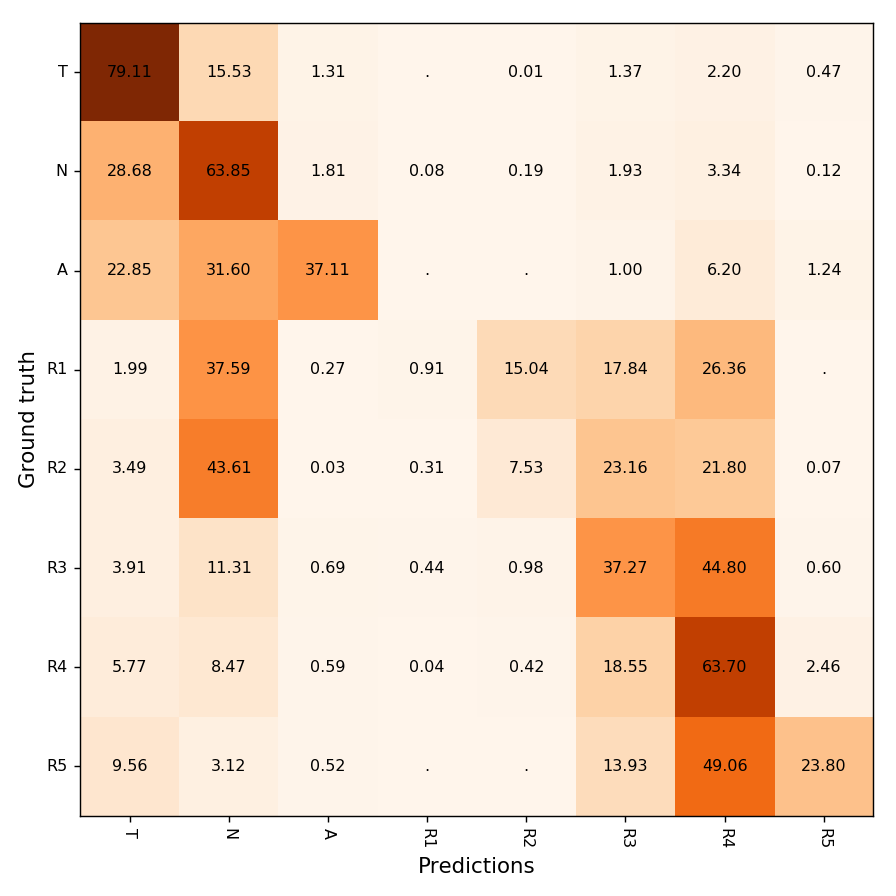
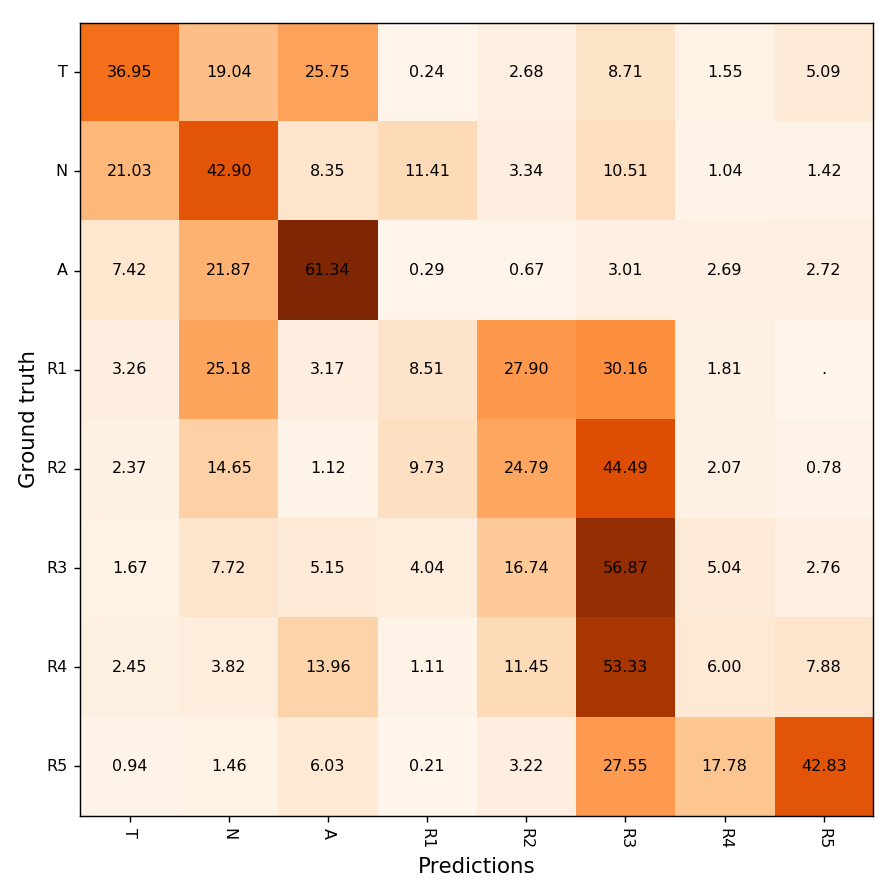
Figure 3: Confusion matrices for the VGG19 (left) and ResNet50 (right) architectures in the multi-class setting. Models trained on the $40\times$ magnification.

6.2 Examination of factors limiting the performance of the convolutional neural networks

In the second stage of the conducted experimental study we analysed some of the factors that might have limited the performance achieved by convolutional neural networks in the patch recognition task. Once again due to the computational constraints we focused on two architectures: VGG19, the model that achieved the best performance in the binary setting in the previous stage of experiments, and ResNet50, as an representative of a more recent architecture that underperformed in the conducted tests. We distinguished three factors that might have affected the performance of a specific neural networks: availability of data, presence of label noise, and data imbalance.

Availability of data. A known difficulty with using machine learning algorithms in the histopathology is high cost associated with data acquisition, which requires a tedious and time-consuming labeling by an experienced medical practitioner. As a result, the availability of the labeled scans is limited. Despite the fact that due to their high resolution the number of image patches extracted from a single scan can be relatively high, an argument can be made that the patches extracted from a single scan are likely to be roughly similar. At the same time, there is a great variation in the appearance of cancer tissue, which makes the process of generalizing from a limited amount of data difficult.

To experimentally evaluate the impact of the amount of available data on the performance of a network trained in the patch recognition task we artificially decreased the number of training observations and retrained the model from scratch, afterwards evaluating its performance on a fixed validation set in the binary class setting. Specifically, we considered the number of scans in $\{6,21,36,51,...,156\}$, incrementally adding 15 training scans to the pool at each evaluation stage. We examined both VGG19 and ResNet50 architectures, and the data was extracted at two different magnifications: $40\times$ and $10\times$. It is worth noting that despite the same pool of scans used for both magnifications, due to the used patch extraction procedure, the total number of patches was approximately 10 times higher at the $40\times$ magnification.

The results of this experiment were presented in Figure 4. Several observations can be made based on the obtained results. First of all, VGG19 network outperformed ResNet50 architecture regardless of the amount of supplied data, scan magnification or chosen performance metric, which is consistent with the results from the previous experiments. Secondly, while the performance of VGG19 network increased monotonically (with the exception of AvAcc at $40\times$ magnification, for which a slight oscillations were present), a much higher variance was observed for ResNet50: this suggests a higher susceptibility of this model to not only quantity but also the quality of data, causing the training to be less stable. This is pronounced even further when considering the AvAcc metric, indicating that in particular the performance on the minority classes is affected. Finally, while the performance of VGG19 to a large extent saturates at the higher number of training scans, in particular at the $40\times$ magnification, for which more patches are available, the performance of ResNet50 kept improving, albeit with large oscillations. It is unclear whether further increase in the number of training scans would decrease the gap in performance between the two architectures.

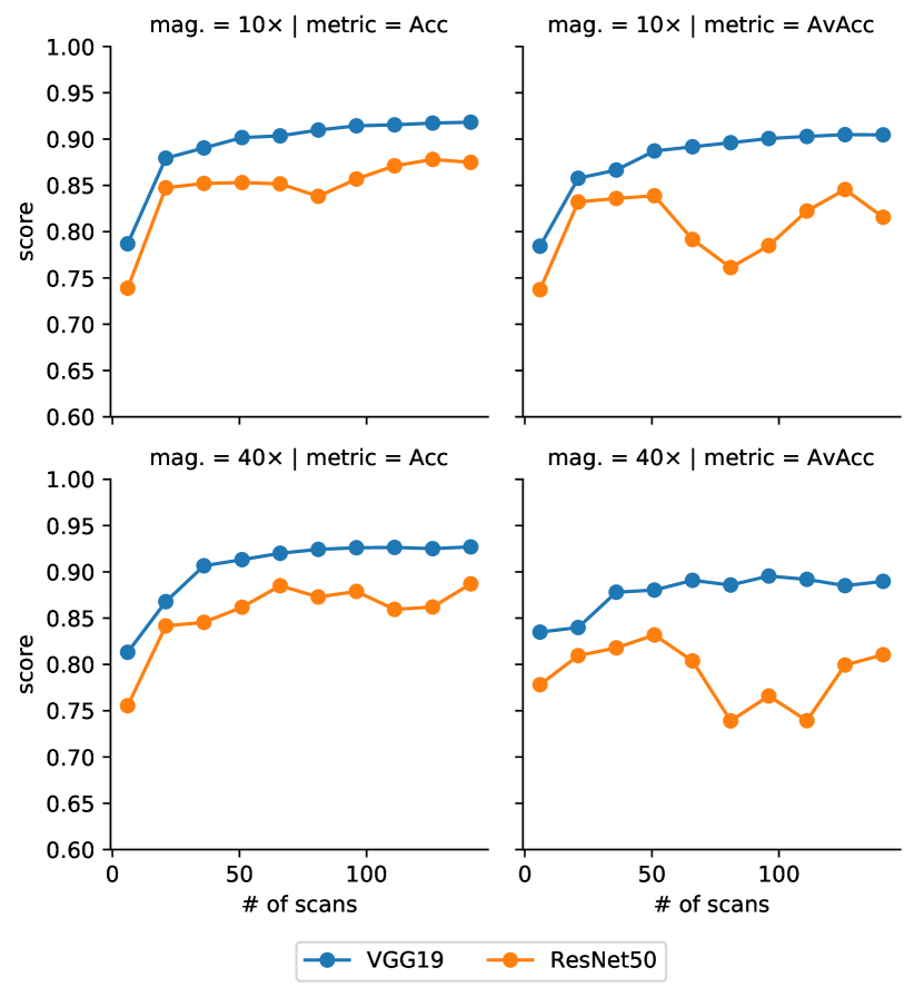
Figure 4: Visualization of the impact of increasing amount of training data (measured as the number of scans from which the patches were extracted) on the classification performance.

A common strategy for reducing the negative impact of low quantity of the available data is using transfer learning, in particular weight transfer from a model trained on another task. However, it is not clear to what extent weight transfer is suitable with a significantly different problem domains of the source and target models, which is the case for an original model trained on a natural image dataset, such as ImageNet, later transferred to the histopathological image recognition task. To experimentally evaluate the usefulness of weight transfer in such scenario we compared the final performance of models either trained from scratch, or initialized with the weights transferred from a model trained on the ImageNet dataset. We examined all possible magnifications, once again using VGG19 and ResNet50 as underlying models in the binary class setting. The observed results were presented in Figure 5. As can be seen, in every single case model trained using weight transfer achieved better performance than the same model trained from scratch, both with respect to accuracy and average accuracy of the predictions. This indicates the suitability of transfer learning, even when the original model was trained on a vastly different problem domain.

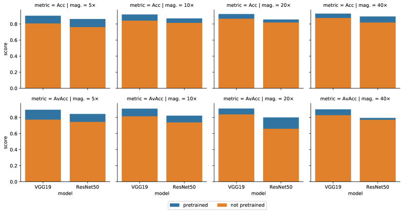
Figure 5: Visualization of the impact of applying weight transfer, with the weights extracted from a model trained on the ImageNet dataset.

Presence of label noise. Another data difficulty factor likely to affect the performance of models in the histopathological image recognition task is presence of label noise. Gleason grading can be a highly subjective task, even at the level of the whole slide. But even more difficulty is associated with the labeling of a specific regions: a number of cases in which medical practitioners labeled different regions as containing cancerous tissue, despite achieving the same diagnosis on the level of the whole scan, was observed during the data acquisition process. Yet another factor contributing to the presence of label noise is the difficulty associated with the exact labeling of intertwining cancerous and non-cancerous tissue: medical practitioners tend to operate on lower magnifications levels than those considered by the proposed patch recognition system, which leads to labeling cancerous regions as a whole, without exclusion of small tissue patches that by itself might not be categorized as cancerous.

As a result of the aforementioned factors, presence of label noise is very likely in the considered data, but both its degree and its impact on the models’ performance remain unknown. However, in an attempt at evaluating said impact we conducted an experiment, in which we artificially introduced label noise to the original data. Specifically, we considered the binary classification setting at several noise levels, and introduced the label noise by randomly changing the label of a given observation to another class with a probability equal to noise level $\in\{0.02,0.04,...,0.20\}$. It is worth noting that due to the inherent data imbalance, with more than twice patches being originally labeled as non-cancerous, described procedure actually decreased the degree of imbalance proportionally to the noise level. The observed results were presented in Figure 6. As can be seen, presence of label noise has a significantly higher impact on the performance for ResNet50 architecture than it does for VGG19. Furthermore, for both of the considered models the negative impact was higher with respect to the AvAcc than the standard accuracy, indicating that even though the proportion of majority observations in the dataset decreased, model became more heavily biased towards the majority class.

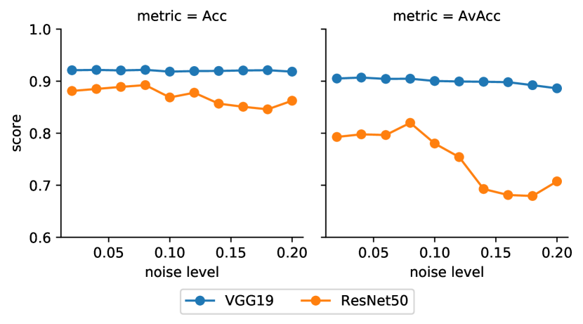
Figure 6: Visualization of the impact of label noise level on the classification performance.

Data imbalance. Finally, yet another data difficulty factor affecting the presented dataset is presence of data imbalance: a disproportion between the number of observations belonging to individual classes. Data imbalance is known to negatively affect the performance of various classification algorithms, including convolutional neural networks (Buda et al., 2018). Several studies (Koziarski et al., 2018; Kwolek et al., 2019; Koziarski, 2019) considered the subject of data imbalance in small-scale histopathological image recognition, with smaller benchmark datasets used as a basis for evaluation. It is however worth noting that data imbalance poses a particular challenge for smaller datasets, in which the number of observations from the minority class might be insufficient to enable successful learning. To evaluate to what extent data imbalance affects the dataset proposed in this paper, and in particular whether the traditional methods for dealing with data imbalance are suitable for reducing its negative impact, we conducted two experiments. First of all, we compared a traditional training strategy of convolutional neural network with batch balancing, an approach in which at each training iteration batch of images is sampled randomly, with artificially introduced even class distribution. Batch balancing is conceptually very similar to random oversampling (ROS) in the mini-batch training mode, with the only difference between the two being the fact that ROS freezes the minority observations that will be over-represented during the initial oversampling, whereas batch balancing over-represents each observation at an equal rate. Both methods were applied in the multi-class Gleason setting, in which every Gleason grade was considered separately, and the remaining classes (T, N and A) were merged into a single non-cancerous class. The results of this experiment were presented in Table 6. As can be seen, by using the batch balancing strategy we were able to improve the performance of a network with respect to AvAcc at 3 out of 4 magnifications. However, in every case applying batch balancing also led to a worst classification accuracy, indicating that the performance in recognition of minority classes was increased at the expense of majority classes. The improvement of performance for minority classes was also not substantial, which was further illustrated with a comparison of confusion matrices of predictions of the network trained in both modes at $40\times$ magnification.

Table 6: Comparison of the performance of a VGG19 network trained with an imbalanced data distribution with a network trained using batch balancing strategy.

Metric	Magnification	Imbalanced	Balanced
Acc	$40\times$	84.56	81.78
	$20\times$	83.97	80.31
	$10\times$	82.73	77.93
	$5\times$	79.80	75.45
AvAcc	$40\times$	35.57	37.10
	$20\times$	38.89	39.26
	$10\times$	39.76	39.54
	$5\times$	38.93	39.80

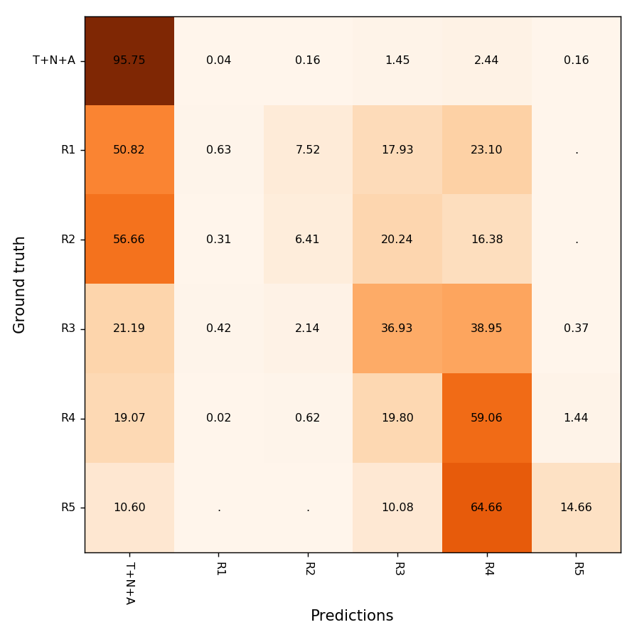
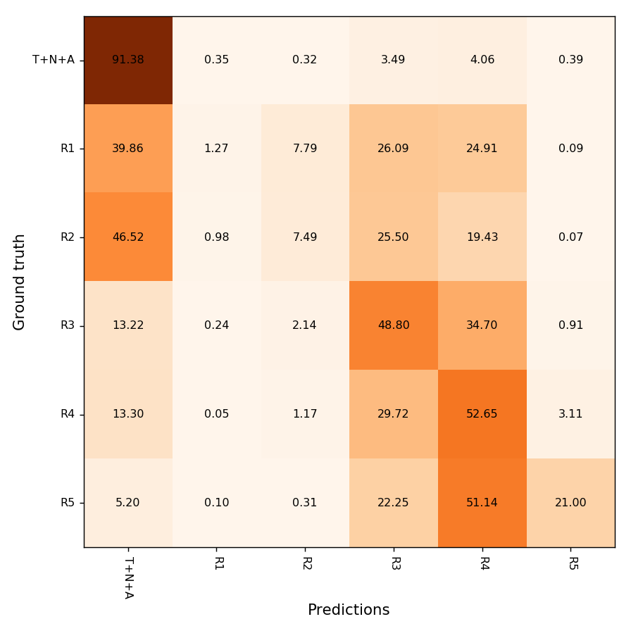
Figure 7: Confusion matrices of predictions made by a network trained in a default training mode (left) and a network trained using batch balancing strategy (right).

Secondly, we evaluated various data-level approaches for handling data imbalance. Specifically, we considered the case in which high-level image features were extracted from the last fully-connected layer of a previously trained VGG19 network, training data was resampled in the feature space, and finally the oversampled, high-level features were classified using a separate SVM classifier with the RBF kernel. High-level features were used instead of the original image representation due to the fact that image data is ill-suited for traditional interpolation-based techniques, such as SMOTE (Chawla et al., 2002). In this stage of experiments we considered several oversampling algorithms: random oversampling (ROS), previously mentioned SMOTE, SMOTE combined with Tomek links (SMOTE+TL) (Tomek, 1976), Borderline SMOTE (Bord) (Han et al., 2005) and CCR (Koziarski et al., 2020). As a reference, we also included the case in which no oversampling was performed (None). In every case, oversampling was performed on a 4096-dimensional feature vector extracted from a previously trained convolutional neural network. Due do the computational limitations, in this stage of the experiments we only considered $10\times$ and $5\times$ magnifications. At this stage we used a complete multi-class setting, that is every class was considered separately. Results were presented in Table 7. As can be seen, using this approach we were able to achieve a greater improvement in performance with respect to AvAcc than the one observed when using batch balancing strategy, with CCR achieving the best results. However, this improvement was accompanied by a larger decrease in standard classification accuracy, which in general was greater for the methods that achieved better AvAcc. While this is an expected behavior, this illustrates the point that despite the fact that improvement in performance on minority classes is possible, it is usually accompanied by a decrease in performance on majority classes. This is important in particular in the problem domain of histopathological image classification, where it is not clear what cost is associated with incorrect classification of minority classes, and in particular how the cost changes depending on whether we are interested only in the binary diagnosis, or we need a specific Gleason discrimination.

Table 7: Comparison of different data oversampling strategies applied prior to SVM-based classification.

Metric	Magnification	None	ROS	SMOTE	SMOTE+TL	Bord	CCR
Acc	$10\times$	66.93	64.05	64.19	63.93	61.59	58.38
	$5\times$	65.18	61.19	61.12	60.72	58.72	56.40
AvAcc	$10\times$	42.69	45.71	44.78	44.81	43.61	48.73
	$5\times$	40.42	41.85	41.29	41.23	40.72	43.10

Conclusions. Based on the results of the conducted experiments it can be concluded that lack of data, presence of label noise and data imbalance are all factors that influence the performance of convolutional neural networks in the patch recognition task. Furthermore, some of those factors tended to have a higher negative impact on ResNet50, used as an example of deeper, more recent architecture, than it did on VGG19. This suggests that the resilience of VGG19 to said factors can make it more suitable for this specific problem domain, and highlights the necessity of development of novel architectures and training strategies, less prone to the negative impact of data difficulty factors.

6.3 Building ensembles of convolutional neural networks

A common strategy for improving the performance of machine learning models is building the classifier ensembles, an approach that combines outputs of several underlying models to form a single, combined prediction. An essential requirement for achieving an improvement in performance when using ensembles is ensuring sufficient diversity of predictions of the underlying models: in the context of computer vision and deep learning, this is often achieved by combining several different architectures of convolutional neural networks. Indeed, as previously demonstrated in Section 6.1, different models can achieve a significantly different performance on specific classes. However, in addition to achieving diversity by combining different neural architectures, histopathological tissue classification in principle enables ensembling of models trained on different tissue magnification. To empirically test the practical usefulness of such approach we conducted an experiment, in which we combined various convolutional neural networks, differing with respect to both the neural architecture, as well as the considered tissue magnification. Specifically, we once again considered AlexNet, VGG16, VGG19, ResNet50 and InceptionV3 networks, each trained on either $40\times$, $20\times$, $10\times$ or $5\times$ magnification. Afterwards, the probabilities returned by the individual models where combined via averaging, either at the model or magnification level, or both. The task considered was the binary classification, that is a discrimination between the cancerous and non-cancerous patches, and the performance was evaluated using standard classification accuracy. The results were presented in Table 8. As can be seen, both ensembling strategies produced results better than the individual models: for the family of models trained on a single magnification, ensembling all 5 architectures produced the best results in the case of every magnification. Similarly, the performance of specific models was also improved in every case by combining different magnifications: depending on the model either combining all of the available magnifications, or all but $5\times$ magnification (on which models tended to achieve the worst performance), produced the best results. Finally, the best overall performance was achieved by combining both modes of ensembling, that is for an ensemble of all available architectures trained on $40\times$, $20\times$ and $10\times$ magnifications, indicating that ensembling on a magnification and model level are complementary.

Table 8: Results achieved by an ensemble of different neural architectures and/or different magnification factors.

Model	$40\times$	$20\times$	$10\times$	$5\times$	$40{+}20\times$	$40{+}20{+}10\times$	$40{+}20{+}10{+}5\times$	$20{+}10\times$	$20{+}10{+}5\times$
AlexNet	89.66	91.07	89.51	83.98	91.98	92.67	92.28	91.86	90.94
VGG16	92.47	93.14	91.57	88.15	94.03	94.26	93.97	93.49	92.55
VGG19	92.32	93.16	91.67	87.92	94.01	94.15	93.87	93.55	92.58
ResNet50	88.29	87.20	88.14	86.20	90.02	91.86	93.14	91.53	92.00
InceptionV3	86.09	90.50	86.45	87.12	90.60	92.96	93.54	92.42	92.29
5 CNN ensemble	92.99	93.74	92.28	88.48	94.22	94.51	94.31	93.86	93.13

It is also worth mentioning that in the patch recognition task predictions made for spatially nearby patches are not uncorrelated: since cancerous tissue tends to form larger clusters containing multiple tissue patches, the presence of non-cancerous neighbors decreases the probability of a given patch being cancerous itself. Because of that, an alternative to traditional ensembling of predictions produced by multiple models can be correcting the predictions of a single model based on the predictions made for neighboring patches. A conceptually simple implementation of this idea is applying median filtering to post-process the prediction map produced by a given model, an approach aimed specifically at eliminating individual outliers that do not form larger clusters. To empirically evaluate the usefulness of such approach we repeated the previously described ensembling experiment, this time post-processing the prediction maps produced by every individual model or ensemble via median filtering with kernel size $k=3$. The results were presented in Table 9. As can be seen, applying median filtering allowed us to achieve a slightly better performance for the ensemble consisting of all of the considered neural architectures and $40\times$, $20\times$ and $10\times$ magnifications. Furthermore, perhaps more importantly, it allowed us to achieve the same performance for an ensemble consisting of a significantly lower number of models, namely two VGG16 networks trained at $40\times$ and $20\times$ magnifications, significantly reducing the computational overhead associated with training and interference. However, it is worth noting that to enable the use of median filtering the classification problem had to be binarized, and extending it to the multi-class setting would require further extensions. Nevertheless, overall the observed results indicate the usefulness of classifier ensembles in the patch recognition task. In particular, both ensembling models trained on different data magnifications, as well as spatially correcting the predictions of the model, seem to offer a suitable alternative to traditional ensembling across different model architectures.

Table 9: Results achieved by a different ensembling strategies, with median filtering applied after the ensembling.

Model	$40\times$	$20\times$	$10\times$	$5\times$	$40{+}20\times$	$40{+}20{+}10\times$	$40{+}20{+}10{+}5\times$	$20{+}10\times$	$20{+}10{+}5\times$
AlexNet	93.20	92.97	90.02	84.16	93.76	93.68	93.00	92.82	91.50
VGG16	94.26	94.19	91.92	88.25	94.67	94.66	94.19	93.96	92.81
VGG19	94.28	94.18	92.00	88.00	94.66	94.54	94.11	94.00	92.80
ResNet50	89.75	89.08	88.65	86.37	91.09	92.29	93.49	92.35	92.47
InceptionV3	85.69	92.37	87.24	87.28	90.83	93.53	93.91	93.41	92.77
5 CNN ensemble	93.92	94.55	92.58	88.56	94.59	94.67	94.53	94.23	93.34

6.4 Evaluation of the final model in the patch recognition task

To avoid the overfitting all of the results presented up to this point were obtained on the validation partition of the dataset. However, to serve as a reference point for further studies we also evaluated the performance of the final model on the test partition of the data. Additionally, compared to the previous experiments which used the DiagSet-A.1 version of the dataset, final performance was reported after training on the DiagSet-A.2, which contained a total of 346 annotated WSI. We examined the performance of an ensemble consisting of VGG19 models trained separately on $40\times$, $20\times$, $10\times$ and $5\times$ magnifications. We evaluated five different class settings, each with a different level of granularity, summarized in Table 10.

Table 10: Summary of different class combination settings (S1-5). Numbers in a given row indicate to which class group given class belongs in that setting.

	BG	T	N	A	R1	R2	R3	R4	R5
S1	1	1	1	1	2	2	2	2	2
S2	1	1	1	1	1	1	2	2	2
S3	1	1	1	1	1	1	2	3	4
S4	1	1	1	1	2	3	4	5	6
S5	1	2	3	4	5	6	7	8	9

Class settings 1 and 2 correspond to the binary classification, with Gleason grades 1 and 2 treated as either cancerous or non-cancerous tissue. In setting 3 additional discrimination between Gleason grades 3-5 was introduced, and grades 1-2 were added to the non-cancerous class group. In setting 4 every Gleason grade was assigned a separate class. Finally, in setting 5 we also introduced the discrimination between the non-cancerous classes, treating each of them separately.

The summary of the results was presented in Table 11, whereas a detailed confusion matrix of the predictions was presented in Figure 8. As can be seen, in all but the last setting, in which a discrimination between non-cancerous tissue classes was introduced, an above 90 percent classification accuracy was observed, with the best performance observed in the first binary setting, for which 94.58 accuracy and 94.70 AvAcc were achieved. The differences between settings 1 and 2 were generally negligible due to a low percentage of scans containing Gleason grades 1 and 2. It is worth noting that the majority of inter-errors was observed between the healthy tissue (N) and tissue background (T), likely due to the fact that non-cancerous regions were labeled in less detail, introducing the largest degree of label noise between those two classes; and Gleason grades 3-5, the discrimination between which was in general more subjective than the discrimination between cancerous and non-cancerous tissue. It is also worth noting that the model in almost no case was able to recognize Gleason grades 1 and 2, labeling them as either healthy tissue or Gleason 3-4 instead. A similar behavior was also displayed for the artifacts, which in most classes were categorized as a healthy tissue.

Table 11: Final performance of the selected model on test partition in patch recognition task, in one of the 5 class settings.

Metric	S1	S2	S3	S4	S5
Acc	94.58	94.53	92.70	92.00	69.36
AvAcc	94.70	94.41	62.91	42.17	44.92

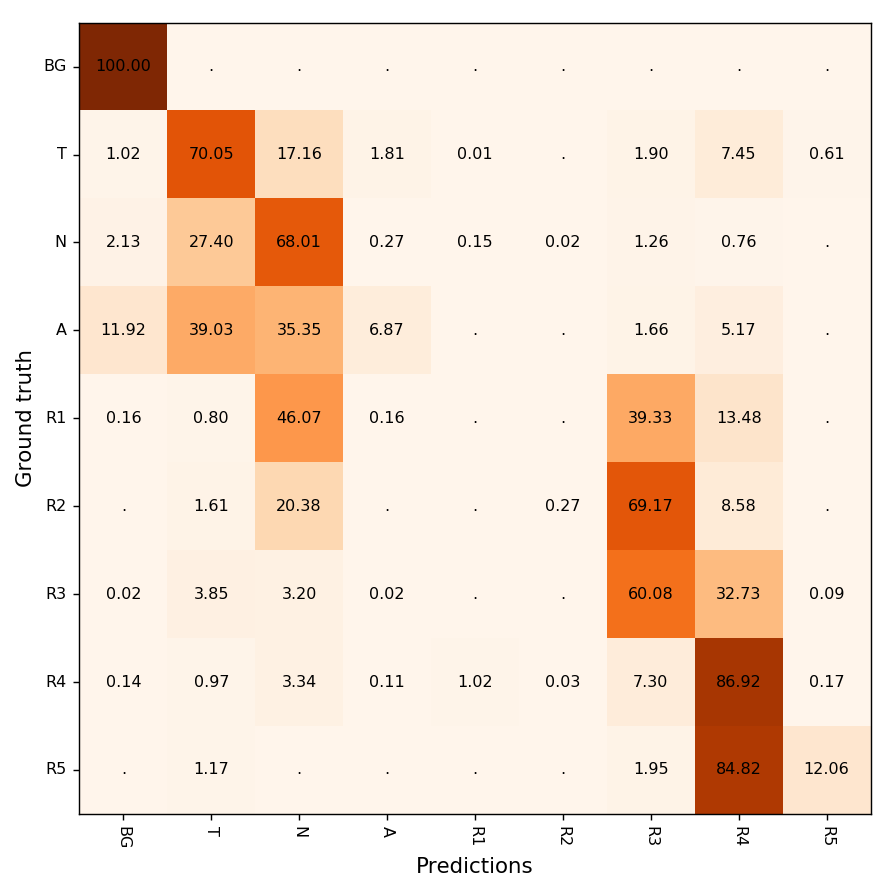
Figure 8: Confusion matrix of the final model in patch recognition task, calculated on the test partition.

6.5 Evaluation of the capabilities of a complete system in the scan-level diagnosis

In addition to evaluating the performance of the proposed methodology in the patch recognition task, we also considered the problem of predicting a final diagnosis for a complete WSI scan. We focused on the binary diagnosis, that is classifying the scan as either cancerous or non-cancerous, with the possibility of abstaining from making the decision in uncertain cases, implying that either further confirmation by human histopathologist or scheduling IHC is necessary. We conducted our analysis on the DiagSet-B dataset, which consisted of 4,675 WSI scans with an associated binarized diagnosis made by a human histopathologist. We began by examining the distribution of percentage of tissue patches classified as cancerous by the ensemble of convolutional neural networks described in Section 6.4. This distribution was presented in Figure 9. As can be seen, there is a clear percentage cut-off, after which every scan in the considered dataset was diagnosed as cancerous by a human histopathologist, and it lies at about 13% of tissue classified as cancerous by the considered ensemble. However, such unambiguousness was not observed in the lower range of the detected cancerous tissue percentage. Still, regions in which one of the diagnosis dominated can be distinguished at around $(0,2)$ and $(5,13)$, indicating some discriminatory capabilities. Finally, neither of the diagnosis dominated in the $(2,5)$ region, clearly indicating the need of abstaining from the diagnosis.

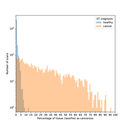
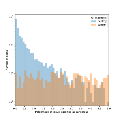
Figure 9: Relation between the percentage of tissue classified as cancerous and ground truth diagnosis given by the histopathologist: in the full range (left) and magnified in the 0-5% range (right). Note that the logarithmic scale was used.

Based on the observed distribution we considered an approach for scan-level diagnosis described in Section 4, which relied on the statistical distribution of predictions made for a given scan in the patch recognition task. To reiterate, the proposed approach was based on a simple decision-making rule using two parameters, lower threshold $T_{L}$, and upper threshold $T_{U}$, that based on the percentage of valid tissue patches (that is, all patches excluding BG class and scan background excluded during the initial segmentation step) of a given scan $p_{c}$, gave a diagnosis ’non-cancerous’ if $p_{c}\leq T_{L}$, ’cancerous’ if $p_{c}\geq T_{U}$, and abstained from making the decision if $T_{L}<p_{c}<T_{U}$

Two matrices, containing the impact of the parameters on both the accuracy and the proportion of scans for which a diagnosis was given, are presented in Figure 10. As can be seen, by properly setting the threshold values we are able to achieve a desired trade-off between the quality and the quantity of the predictions. For example, setting the lower threshold at 0.5% and the upper threshold at 7%, which corresponds to the case in which we diagnose a scan as cancerous if the percentage of patches classified as cancerous is lower than 0.5%, as non-cancerous if it is higher than 7%, and we abstain from making the decision in the remaining cases, we achieve a 99.04% diagnosis accuracy, at the same time processing 73.16% of scans, or in other words abstaining from making the decision for 26.84% of the scans. On the other hand, in the extremes we are able to achieve either a perfect diagnosis accuracy on the considered dataset, in which case, however, we only process 31.59% of the scans, or process almost all of the scans, that is 98.59% of them, at the same time achieving a lower diagnosis accuracy of 93.92%. The observed results indicate that while using a simple decision rule, in which we base the diagnosis on the percentage of tissue classified as cancerous, is not sufficient to achieve a perfect performance for all of the cases, by properly setting the range in which we abstain from giving the diagnosis we can significantly improve the performance at the cost of the number of processed scans. In particular, the scans for which a high percentage of tissue was classified as cancerous led to a high certainty of correct diagnosis, whereas more ambiguity was present at the opposite end of the spectrum, at which even a very small number of cancerous patches could have indicated the actual presence of cancer. As a result, this suggests the suitability of the system for the initial screening, during which we give the diagnosis only for the scans we deem least ambiguous.

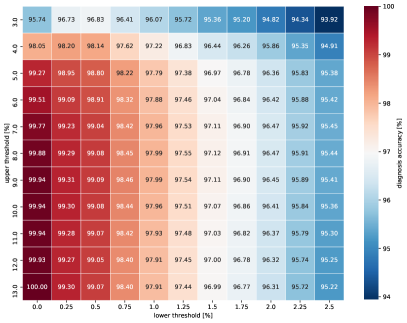
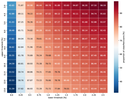
Figure 10: The impact of setting the lower and upper threshold used to give a final diagnosis on the diagnosis accuracy (left) and the proportion of classified scans (right).

6.6 Evaluation based on the statistical hypothesis testing

As mentioned before, the series of patch probabilities returned by the neural networks operating over an WSI can be treated as a random variable following a certain probabilistic distribution. Therefore, the problem of WSI classification can be interpreted as verification of a statistical hypothesis. For this purpose in our work one parametric and two non-parametric statistical hypothesis tests were investigated, as described in Section 5. However, results of a direct classification with this approach, although concordant between the three statistical hypothesis methods, were worse than the ones presented with the threshold based decision method described in Section 6.5. Nevertheless, we noticed that these statistical test can be used to accompany the threshold based decision method as a kind of a post-hoc assessment. In other words, after the threshold based response is given, this strategy allows to further verify a hypothesis if a statistical sample of a given test WSI does agree, or does not agree, with the distribution of the entire population of the samples obtained by grouping all patch probabilities from the WSI scans which have been assigned the cancer (C) or no-cancer (NC) label by the histopathologists. Such statistical tests can allow to distinguish statistically deviating cases and indicate e.g. a necessity of additional examinations.

In the experiments 418 WSI scans for C (cancer), and 517 for NC (no-cancer), were used, respectively. From these 80% were used to build the reference patch populations, whereas the remaining 20% were used for the method assessment ("Train %" in Table 13). For the former group the patch probabilities returned by the ensemble of the convolutional neural networks described in Section 6.5 have been gathered into the two populations. Histograms of this way obtained populations C and NC are shown in Figure 11, respectively. It is well visible that these are highly tailed distributions, both with the prevailing left tail, and the smaller but observable right tail in the case of the C population. The larger left tail in both distributions corresponds to the high number of healthy tissue patches, which can be encountered in both C, as well as NC, scans. This left tail is common to the two populations since even NC scans contain usually a large amount of healthy tissues. The right tail, on the other hand, corresponds to a significant amount of the cancerous patches, prevailing in the C population. Hence, since we wish to well distinguish the two groups we decided to cut off the common left tail by taking only the 2nd quantile of each of the populations. Their histograms are shown in Figure 12. Detailed values of the number of the WSI scans used in these experiments, as well as the patches that form the C and NC populations are included in Table 12. For the diagnosis, the algorithm described in Section 5 has been used with the parameters shown in Table 13.

Results for the three statistical tests performed for these two groups are shown in Table 14. We can conclude that 27-30% of the C test samples did not have enough statistical support for the hypothesis that they belong to the C population. This factor within the group of NC test samples is in the range 2-3%. On the other hand, there are no errors of type II, i.e. misclassifications. This can indicate that the proposed post hoc statistical verification of the diagnosis can be used to select the cases that significantly differ from the population and which may require further examination, such as the IHC.

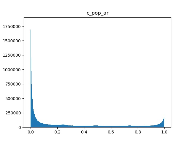
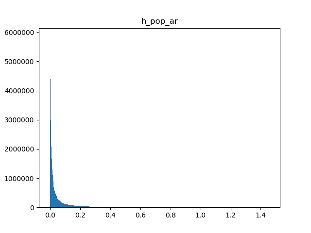
Figure 11: Histograms of the patch probabilities of the cancer (left) and healthy (right) tissues.

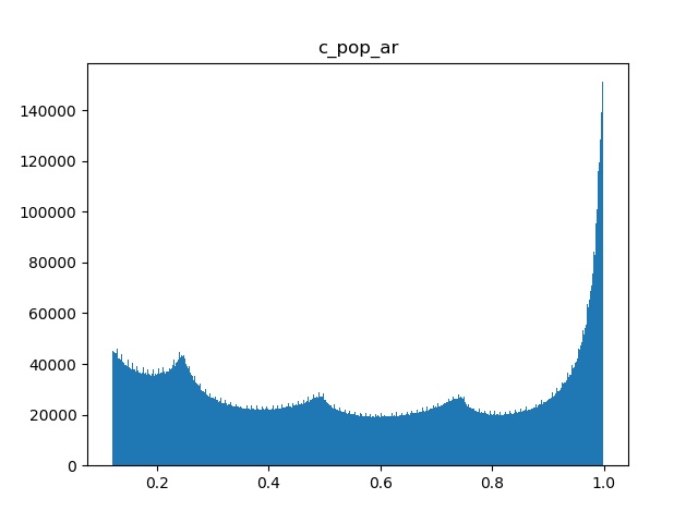
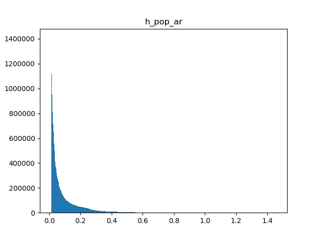
Figure 12: Histograms of the patch probabilities of the 2nd quantile of the cancer (left) and healthy (right) tissues.

Table 12: Parameters of the experimental database.

Parameter	#C	#NC
No. WSI	2090	2585
No. patch	26.320.040	29.524.239
No. patch above $q$	13.160.481	14.803.454

Table 13: Parameters used in the statistical hypothesis test experiment.

Parameter	Description	Value
Train %	Patch population size expressed as a percentage of all available annotated patch probabilities	80%
Repetitions	A number of repetitions of the entire experiment	10
Cut-off quant	Population cut-off value	$q$=0.5
Single sample size	Size of the drawn sample at each test	s=20
No of draws for a test	No of repetitions of each test on a randomly drawn sample	$n$=1000
Pass overhead	Provides an overhead of passed vs. failed statistical test within a group of repetitions ns.	$r$=5%

Table 14: Results of the post-hoc statistical tests performed on 418 of the test cancer and 517 test healthy WSI.

Test / Parameter	C-I	C-II	NC-I	NC-II
Welch t-test	124 (30%)	0	9 (2%)	0
WMW	112 (27%)	0	10 (2%)	0
Permutation	113 (27%)	0	14 (3%)	0

6.7 Comparison with human histopathologists

To assess coherence of the medical diagnosis of the prostate cancer an experiment with 9 volunteered physicians, experts in histopathology, has been conducted. They have been presented with the 46 WSI of prostate tissue, some containing canerous changes. The same has been tried with the DCNN diagnosis rule presented in Section 6.5. Results of this experiment are presented in the Table 15. Each Di column contains responses of the i-th expert, whereas DCNN corresponds to the responses of the proposed system. The "C Tissue %" column reflects the percentage of the cancerous tissues in each WSI scan as returned by the ensemble of deep classifiers. The last three columns of Table 15 contain classification results obtained with the statistical hypothesis tests: the Welch parametric t-test, as well the nonparametric WMW and the permutation test, as described in Section 5. In this case, each of the statistical hypothesis tests was performed independently from each other and the DCNN (i.e. this is not the post hoc procedure described in the previous section), and the diagnosis was given based on the algorithm described in Section 5.

At least two interesting observations can be made. First, that the three statistical tests are concordant on a vast majority of the scans with the only one difference for the WSI no. 27, which is the only one for which all machine decisions are different from the decisions made by the experts. The second observation is a difference between the statistical tests and the DCNN. In this case the answers are also highly concordant except for the few cases, wherein only differences between the IHC and NC or IHC and C, but never between C and NC, can be observed, however. This comes from differences in the abstaining rules of each of these methods.

The list of the WSI IDs used in the experiment shown in Table 15 is contained in the additional materials accompanying this paper.

Table 15: Results of the experiment of the prostate cancer diagnosis experiment performed by the nine histopathology experts Di, DCNN and the three statistical hypothesis tests. "C Tissue %" contains a percentage of cancerous tissues detected by the ensemble of deep classifiers.

WSI No.	D1	D2	D3	D4	D5	D6	D7	D8	D9	C Tissue %	DCNN	Welch	WMW	Permut
1	C	C	C	C	C	C	C	C	C	13.35	C	C	C	C
2	C	C	C	IHC	C	C	C	C	C	21.77	C	C	C	C
3	C	C	C	C	C	C	C	C	C	13.78	C	C	C	C
4	C	C	C	C	C	IHC	C	C	C	10.90	C	C	C	C
5	C	C	C	C	C	C	C	C	C	35.16	C	C	C	C
6	C	C	C	C	C	C	C	C	C	34.80	C	C	C	C
7	C	C	C	C	C	C	C	C	C	46.16	C	C	C	C
8	C	C	C	C	C	C	C	C	C	46.78	C	C	C	C
9	C	C	C	C	C	C	C	C	C	24.83	C	C	C	C
10	C	IHC	NC	C	NC	NC	NC	IHC	IHC	1.87	IHC	NC	NC	NC
11	C	C	C	C	C	C	C	C	C	33.22	C	C	C	C
12	C	C	C	C	C	C	C	C	C	3.90	IHC	NC	NC	NC
13	C	C	IHC	IHC	NC	IHC	IHC	C	C	0.33	NC	NC	NC	NC
14	NC	NC	NC	NC	NC	NC	NC	IHC	NC	0.00	NC	IHC	IHC	IHC
15	C	NC	IHC	IHC	IHC	NC	IHC	IHC	IHC	0.15	NC	NC	NC	NC
16	NC	NC	NC	NC	NC	NC	NC	NC	NC	0.06	NC	NC	NC	NC
17	C	C	C	C	C	C	C	C	C	25.04	C	C	C	C
18	C	C	C	C	C	C	C	C	C	46.00	C	C	C	C
19	IHC	IHC	NC	IHC	NC	IHC	NC	IHC	IHC	2.16	IHC	NC	NC	NC
20	IHC	IHC	NC	IHC	NC	NC	NC	NC	IHC	0.09	NC	NC	NC	NC
21	IHC	IHC	NC	IHC	NC	IHC	IHC	IHC	IHC	1.33	IHC	NC	NC	NC
22	C	C	C	C	C	C	C	C	C	8.51	C	C	C	C
23	C	C	C	C	C	C	C	C	C	69.31	C	C	C	C
24	IHC	C	C	C	C	C	C	C	C	2.55	IHC	NC	NC	NC
25	IHC	C	C	IHC	C	C	C	C	C	2.46	IHC	NC	NC	NC
26	IHC	C	C	C	C	C	C	C	C	3.49	IHC	IHC	IHC	IHC
27	C	C	C	C	C	C	C	C	C	5.87	IHC	IHC	IHC	NC
28	C	C	C	C	C	C	C	IHC	C	69.49	C	C	C	C
29	C	C	C	C	C	C	C	C	C	54.05	C	C	C	C
30	IHC	C	IHC	C	C	C	C	C	C	8.76	C	IHC	IHC	IHC
31	C	C	C	C	C	C	C	C	C	13.38	C	C	C	C
32	C	C	C	C	C	C	C	C	C	10.02	C	C	C	C
33	IHC	IHC	NC	IHC	NC	NC	NC	IHC	NC	6.42	IHC	IHC	IHC	IHC
34	C	C	C	C	C	C	C	C	C	29.68	C	C	C	C
35	C	C	C	C	C	C	C	C	C	55.96	C	C	C	C
36	C	C	C	C	C	C	C	C	C	37.92	C	C	C	C
37	C	C	C	C	C	C	C	C	C	10.21	C	C	C	C
38	C	C	C	C	C	C	C	C	C	27.60	C	C	C	C
39	C	C	C	C	C	C	C	C	C	14.54	C	C	C	C
40	C	C	C	C	C	C	C	C	C	32.48	C	C	C	C
41	NC	NC	NC	NC	NC	NC	NC	NC	NC	0.39	NC	NC	NC	NC
42	NC	NC	NC	IHC	NC	NC	NC	IHC	IHC	5.13	IHC	IHC	IHC	IHC
43	C	C	C	C	C	C	C	C	C	21.11	C	C	C	C
44	IHC	NC	IHC	NC	IHC	IHC	NC	IHC	IHC	0.13	NC	NC	NC	NC
45	NC	NC	NC	NC	NC	NC	NC	NC	NC	0.49	NC	NC	NC	NC
46	NC	NC	NC	NC	NC	NC	NC	NC	IHC	0.40	NC	NC	NC	NC

Finally, correlations of the answers shown in Table 15 have been statistically verified with the help of the Spearman non parametric test (Sheskin, 2007). Each pair of responses has been verified, including the responses of a human vs. human, as well as human vs. the proposed DCNN rule. Results of these tests are presented in Table 16. The correlation between DCNN method and expert histopatologists is in the range from 0.75 up to 0.83. These results do not significantly differ from the correlations obtained in the group of the human experts, in which the lowest correlation was 0.64.

Table 16: Non parametric Spearman correlation coefficients between the 9 histopathologists and DCNN on examination of 47 WSI with various stadia of the prostate cancer.

	D1	D2	D3	D4	D5	D6	D7	D8	D9	DCNN
D1	1.00	0.73	0.74	0.78	0.68	0.64	0.70	0.70	0.73	0.75
D2	0.73	1.00	0.92	0.82	0.92	0.93	0.95	0.94	0.98	0.79
D3	0.74	0.92	1.00	0.79	0.97	0.93	0.96	0.89	0.93	0.78
D4	0.78	0.82	0.79	1.00	0.82	0.79	0.83	0.77	0.81	0.83
D5	0.68	0.92	0.97	0.82	1.00	0.95	0.99	0.89	0.93	0.82
D6	0.64	0.93	0.93	0.79	0.95	1.00	0.96	0.89	0.93	0.79
D7	0.70	0.95	0.96	0.83	0.99	0.96	1.00	0.92	0.96	0.82
D8	0.70	0.94	0.89	0.77	0.89	0.89	0.92	1.00	0.94	0.74
D9	0.73	0.98	0.93	0.81	0.93	0.93	0.96	0.94	1.00	0.78
DCNN	0.75	0.79	0.78	0.83	0.82	0.79	0.82	0.74	0.78	1.00

7 Conclusions

In this paper we present the DiagSet dataset containing whole slide images of the prostate cancer tissues annotated and labeled by the professional histopathology doctors in accordance with the Gleason scale. This dataset made possible training and testing of a number of deep convolutional neural network architectures, such as AlexNet, VGG16, VGG19, ResNet50, and InceptionV3 in various configurations, data imbalance settings, and different image magnifications. From these the best performing configurations were selected to form an ensemble of deep neural classifiers, for which the obtained best average accuracy is 94.67% in the binary cancer vs. no-cancer classification setup. Apart, the statistical hypothesis testing framework, containing one parametric and two non-parametric methods, has been proposed as the additional diagnosis verification methods. The obtained results of machine based diagnosis have been verified in the experiment involving histopathology doctors, showing high statistical agreement. The DiagSet is available at https://ai-econsilio.diag.pl.

References

- Albelda (1993) Albelda, S.M., 1993. Role of integrins and other cell adhesion molecules in tumor progression and metastasis. Lab. Invest. 68, 4–17.
- Arvaniti et al. (2018) Arvaniti, E., Fricker, K.S., Moret, M., Rupp, N., Hermanns, T., Fankhauser, C., Wey, N., Wild, P.J., Rüschoff, J.H., Claassen, M., 2018. Automated gleason grading of prostate cancer tissue microarrays via deep learning. Scientific Reports 8, 12054. URL: https://doi.org/10.1038/s41598-018-30535-1, doi:10.1038/s41598-018-30535-1.
- Buda et al. (2018) Buda, M., Maki, A., Mazurowski, M.A., 2018. A systematic study of the class imbalance problem in convolutional neural networks. Neural Networks 106, 249–259.
- Bulten and Litjens (2018) Bulten, W., Litjens, G., 2018. Unsupervised prostate cancer detection on H&E using convolutional adversarial autoencoders. arXiv:1804.07098.
- Bulten et al. (2020) Bulten, W., Pinckaers, H., van Boven, H., Vink, R., de Bel, T., van Ginneken, B., van der Laak, J., Hulsbergen-van de Kaa, C., Litjens, G., 2020. Automated deep-learning system for Gleason grading of prostate cancer using biopsies: a diagnostic study. The Lancet Oncology 21, 233–241. URL: http://dx.doi.org/10.1016/S1470-2045(19)30739-9, doi:10.1016/s1470-2045(19)30739-9.
- Campanella et al. (2018) Campanella, G., Silva, V.W.K., Fuchs, T.J., 2018. Terabyte-scale deep multiple instance learning for classification and localization in pathology. arXiv:1805.06983.
- Chawla et al. (2002) Chawla, N.V., Bowyer, K.W., Hall, L.O., Kegelmeyer, W.P., 2002. SMOTE: synthetic minority over-sampling technique. Journal of Artificial Intelligence Research 16, 321--357.
- Choi (2016) Choi, S.W., 2016. Life is lognormal! what to do when your data does not follow a normal distribution. Anaesthesia 71, 1363--1366. URL: https://onlinelibrary.wiley.com/doi/abs/10.1111/anae.13666, doi:10.1111/anae.13666, arXiv:https://onlinelibrary.wiley.com/doi/pdf/10.1111/anae.13666.
- Deng et al. (2009) Deng, J., Dong, W., Socher, R., Li, L.J., Li, K., Fei-Fei, L., 2009. ImageNet: A large-scale hierarchical image database, in: 2009 IEEE conference on computer vision and pattern recognition, IEEE. pp. 248--255.
- Derrick and White (2016) Derrick, B., White, P., 2016. Why welch’s test is type i error robust. The Quantitative Methods for Psychology 12, 30--38. URL: http://www.tqmp.org/RegularArticles/vol12-1/p030/p030.pdf, doi:10.20982/tqmp.12.1.p030.
- Epstein et al. (2005) Epstein, J.I., Allsbrook Jr., W.C., Amin, M.B., Egevad, L.L., , the ISUP Grading Committee, 2005. The 2005 international society of urological pathology (isup) consensus conference on gleason grading of prostatic carcinoma. The American Journal of Surgical Pathology 29. URL: https://journals.lww.com/ajsp/Fulltext/2005/09000/The_2005_International_Society_of_Urological.15.aspx.
- Epstein et al. (2016) Epstein, J.I., Egevad, L., Amin, M.B., Delahunt, B., Srigley, J.R., Humphrey, P.A., Al-Hussain, T., Algaba, F., Aron, M., Berman, D., Berney, D., Brimo, F., Cao, D., Cheville, J., Clouston, D., Colecchia, M., Comperat, E., da Cunha, I.W., De Marzo, A., Ertoy, D., Fine, S., Foster, C., Grignon, D., Gupta, N., Gupta, R., Kench, J., Kristiansen, G., Kunju, L., Leite, K.R., Loda, M., Lopez-Beltran, A., Lotan, T., Lucia, M., Magi-Galluzzi, C., Montironi, R., McKenney, J., Merrimen, J., Netto, G., Orozco, R., Paner, G., Parwani, A., Pizov, G., Reuter, V., Ro, J., Samaratunga, H., Schultz, L., Shanks, J., Sesterhenn, I., Shen, S., Simko, J., Suzigan, S., Suryavanshi, M., Tan, P.H., Takahashi, H., Tomlins, S., Trpkov, K., Troncoso, P., True, L., Tsuzuki, T., van der Kwast, T., Varma, M., Warren, A., Wheeler, T., Yang, X., Zhou, M., Kantoff, P., Eisenberger, M., Stadler, W., Andriole, G., Klein, E., Benson, M., Montorsi, F., Crawford, D., Loeb, S., Catto, J., Schaeffer, E., Nacey, J.N., DeWeese, T., Sandler, H., Zietman, A., Pollack, A., Rodrigues, G., 2016. The 2014 International Society of Urological Pathology (ISUP) Consensus Conference on Gleason Grading of Prostatic Carcinoma: Definition of Grading Patterns and Proposal for a New Grading System. Am. J. Surg. Pathol. 40, 244--252.
- Ernst (2004) Ernst, M.D., 2004. Permutation methods: A basis for exact inference. Statist. Sci. 19, 676--685. URL: https://doi.org/10.1214/088342304000000396, doi:10.1214/088342304000000396.
- Fagerland (2012) Fagerland, M.W., 2012. t-tests, non-parametric tests, and large studies--a paradox of statistical practice? BMC medical research methodology 12, 78--78. URL: https://pubmed.ncbi.nlm.nih.gov/22697476, doi:10.1186/1471-2288-12-78. 22697476[pmid].
- Fagerland and Sandvik (2009) Fagerland, M.W., Sandvik, L., 2009. The wilcoxon–mann–whitney test under scrutiny. Statistics in Medicine 28, 1487--1497. URL: https://onlinelibrary.wiley.com/doi/abs/10.1002/sim.3561, doi:10.1002/sim.3561, arXiv:https://onlinelibrary.wiley.com/doi/pdf/10.1002/sim.3561.
- Fay and Proschan (2010) Fay, M.P., Proschan, M.A., 2010. Wilcoxon-mann-whitney or t-test? on assumptions for hypothesis tests and multiple interpretations of decision rules. Statist. Surv. 4, 1--39. URL: https://doi.org/10.1214/09-SS051, doi:10.1214/09-SS051.
- Gleason (1966) Gleason, D.F., 1966. Classification of prostatic carcinomas. Cancer Chemother Rep 50, 125--128.
- Han et al. (2005) Han, H., Wang, W.Y., Mao, B.H., 2005. Borderline-SMOTE: a new over-sampling method in imbalanced data sets learning, in: International Conference on Intelligent Computing, Springer. pp. 878--887.
- He et al. (2016) He, K., Zhang, X., Ren, S., Sun, J., 2016. Deep residual learning for image recognition, in: Proceedings of the IEEE conference on computer vision and pattern recognition, pp. 770--778.
- Janowczyk and Madabhushi (2016) Janowczyk, A., Madabhushi, A., 2016. Deep learning for digital pathology image analysis: A comprehensive tutorial with selected use cases , 7:29.
- Kim et al. (2016) Kim, J., Kwon Lee, J., Mu Lee, K., 2016. Accurate image super-resolution using very deep convolutional networks, in: Proceedings of the IEEE conference on computer vision and pattern recognition, pp. 1646--1654.
- Konig et al. (2004) Konig, J.E., Senge, T., Allhoff, E.P., K?nig, W., 2004. Analysis of the inflammatory network in benign prostate hyperplasia and prostate cancer. Prostate 58, 121--129.
- Koziarski (2019) Koziarski, M., 2019. Radial-Based Undersampling algorithm for classification of breast cancer histopathological images affected by data imbalance, in: 2019 12th International Congress on Image and Signal Processing, BioMedical Engineering and Informatics (CISP-BMEI), IEEE. pp. 1--5.
- Koziarski et al. (2018) Koziarski, M., Kwolek, B., Cyganek, B., 2018. Convolutional neural network-based classification of histopathological images affected by data imbalance, in: Video Analytics. Face and Facial Expression Recognition. Springer, pp. 1--11.
- Koziarski et al. (2020) Koziarski, M., Woźniak, M., Krawczyk, B., 2020. Combined Cleaning and Resampling algorithm for multi-class imbalanced data with label noise. Knowledge-Based Systems 204, 106223. URL: http://www.sciencedirect.com/science/article/pii/S0950705120304330, doi:https://doi.org/10.1016/j.knosys.2020.106223.
- Krizhevsky et al. (2012) Krizhevsky, A., Sutskever, I., Hinton, G.E., 2012. ImageNet classification with deep convolutional neural networks, in: Advances in neural information processing systems, pp. 1097--1105.
- Kwolek et al. (2019) Kwolek, B., Koziarski, M., Bukała, A., Antosz, Z., Olborski, B., Wąsowicz, P., Swadźba, J., Cyganek, B., 2019. Breast cancer classification on histopathological images affected by data imbalance using active learning and deep convolutional neural network, in: International Conference on Artificial Neural Networks, Springer. pp. 299--312.
- Litjens et al. (2017) Litjens, G., Kooi, T., Bejnordi, B.E., Setio, A.A.A., Ciompi, F., Ghafoorian, M., van der Laak, J.A., van Ginneken, B., Sánchez, C.I., 2017. A survey on deep learning in medical image analysis. Medical Image Analysis 42, 60 -- 88. URL: http://www.sciencedirect.com/science/article/pii/S1361841517301135, doi:https://doi.org/10.1016/j.media.2017.07.005.
- Litjens et al. (2016) Litjens, G., Sánchez, C., Timofeeva, N., Hermsen, M., Nagtegaal, I., Kovacs, I., Hulsbergen-van de Kaa, C., Bult, P., Ginneken, B., van der Laak, J., 2016. Deep learning as a tool for increased accuracy and efficiency of histopathological diagnosis. Scientific Reports 6, 26286. doi:10.1038/srep26286.
- Nagpal et al. (2019) Nagpal, K., Foote, D., Liu, Y., Chen, P.H., Wulczyn, E., Tan, F., Olson, N., Smith, J., Mohtashamian, A., Wren, J., Corrado, G., MacDonald, R., Peng, L., Amin, M., Evans, A., Sangoi, A., Mermel, C., Hipp, J., Stumpe, M., 2019. Development and validation of a deep learning algorithm for improving Gleason scoring of prostate cancer. npj Digital Medicine 2, 48. doi:10.1038/s41746-019-0112-2.
- Nir et al. (2018) Nir, G., Hor, S., Karimi, D., Fazli, L., Skinnider, B., Tavassoli, P., Turbin, D., Villamil, C., Wang, G., Wilson, R., Iczkowski, K., Lucia, M., Black, P., Abolmaesumi, P., Goldenberg, L., Salcudean, S., 2018. Automatic grading of prostate cancer in digitized histopathology images: Learning from multiple experts. Medical Image Analysis 50. doi:10.1016/j.media.2018.09.005.
- Pan et al. (2017) Pan, X., Li, L., Yang, H.H., Liu, Z., Yang, J., Zhao, L., Fan, Y., 2017. Accurate segmentation of nuclei in pathological images via sparse reconstruction and deep convolutional networks. Neurocomputing 229, 88--99.
- Ren et al. (2018) Ren, J., Hacihaliloglu, I., Singer, E.A., Foran, D.J., Qi, X., 2018. Adversarial domain adaptation for classification of prostate histopathology whole-slide images. arXiv:1806.01357.
- Sheskin (2007) Sheskin, D.J., 2007. Handbook of Parametric and Nonparametric Statistical Procedures. 4 ed., Chapman & Hall/CRC.
- Simonyan and Zisserman (2014) Simonyan, K., Zisserman, A., 2014. Very deep convolutional networks for large-scale image recognition. arXiv preprint arXiv:1409.1556 .
- Spanhol et al. (2016) Spanhol, F.A., Oliveira, L.S., Petitjean, C., Heutte, L., 2016. A dataset for breast cancer histopathological image classification. IEEE Transactions on Biomedical Engineering 63, 1455--1462. doi:10.1109/TBME.2015.2496264.
- Srinidhi et al. (2019) Srinidhi, C.L., Ciga, O., Martel, A.L., 2019. Deep neural network models for computational histopathology: A survey. arXiv:1912.12378.
- Szegedy et al. (2016) Szegedy, C., Vanhoucke, V., Ioffe, S., Shlens, J., Wojna, Z., 2016. Rethinking the Inception architecture for computer vision, in: Proceedings of the IEEE conference on computer vision and pattern recognition, pp. 2818--2826.
- Tomek (1976) Tomek, I., 1976. Two modifications of CNN. IEEE Transactions on Systems, Man, and Cybernetics 6, 769--772.
- Vandenberghe et al. (2017) Vandenberghe, M., Scott, M., Scorer, P., Soderberg, M., Balcerzak, D., Barker, C., 2017. Relevance of deep learning to facilitate the diagnosis of her2 status in breast cancer open. Scientific Reports 7. doi:10.1038/srep45938.
- Wan et al. (2017) Wan, T., Cao, J., Chen, J., Qin, Z., 2017. Automated grading of breast cancer histopathology using cascaded ensemble with combination of multi-level image features. Neurocomputing 229, 34 -- 44. URL: http://www.sciencedirect.com/science/article/pii/S0925231216305471, doi:https://doi.org/10.1016/j.neucom.2016.05.084. advances in computing techniques for big medical image data.