Bayesian Kernelised Test of (In)dependence with Mixed-type Variables

Abstract

A fundamental task in AI is to assess (in)dependence between mixed-type variables (text, image, sound). We propose a Bayesian kernelised correlation test of (in)dependence using a Dirichlet process model. The new measure of (in)dependence allows us to answer some fundamental questions: Based on data, are (mixed-type) variables independent? How likely is dependence/independence to hold? How high is the probability that two mixed-type variables are more than just weakly dependent? We theoretically show the properties of the approach, as well as algorithms for fast computation with it. We empirically demonstrate the effectiveness of the proposed method by analysing its performance and by comparing it with other frequentist and Bayesian approaches on a range of datasets and tasks with mixed-type variables.

1 Introduction

Most traditional data analysis approaches are hindered by handling either continuous or categorical variables but not both. The digital era has led to a rapid increase in data diversity and volume. This requires techniques that can effectively deal with mixed-type data (images, text, sound), and that are able to extract useful information from data and to communicate meaningful insights. We focus on a particular aspect of data analysis through the following Question: Given mixed-type variables, are they dependent or are they independent?

Distance correlation (dCor) [19, 20] is a measure of dependence that generalises Pearson correlation defined for paired variables of arbitrary (and not necessarily equal) type. dCor takes values in $[0,1]$ and equals zero if and only if independence holds. It detects both linear and nonlinear associations. Moreover, it has been shown [17] that its statistics can be defined via the squared Hilbert-Schmidt norm of the cross-covariance operator (HSIC) of the kernel embedding of the distribution into Reproducing Kernel Hilbert Spaces (RKHSs) [6, 7, 9, 11, 12]. Therefore, dCor can be easily generalised to any type of data by using kernel embedding. Using dCor statistics, a Null-Hypothesis Significance Test (NHST) of independence can be derived. dCor is potentially a very powerful and interpretative tool to answer our Question but it has two major drawbacks: (i) It has a bias towards dependence that increases with the dimension of the variables being compared (to remove this bias, only an ad-hoc solution has been proposed [21]); (ii) The p-value-based NHST derived from dCor cannot really answer our Question about independence. In NHST, dependence is “declared” whenever the p-value is below a certain significance threshold. P-value is the probability that any dCor generated from the null hypothesis, according to the intended sampling process, has magnitude greater than or equal to that of the observed $\text{dCor}_{obs}$, that is, $\text{p-value}=p(\text{any }\text{dCor}_{null}\geq\text{dCor}_{obs})$. Since a p-value is evaluated only under the null hypothesis, it cannot say anything directly about the comparison between the null and alternative hypotheses. Using a NHST we can never declare that the two variables are independent. Thus, such test is not able to distinguish between statistical and practical significance (that is, the difference between weak and strong dependence).

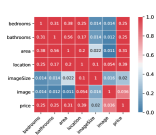
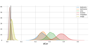
(a)	(b)	(c)

Figure 1: BKR applied to the House dataset. (a) An example of entry; (b) heatmap of BdCor among attributes; (c) Posterior of attributes’ relation with price (ROPI is the region at the left of the black vertical line).

Questions such as those in the abstract are questions about posterior probabilities, which can be naturally provided by the Bayesian methods. We propose a Bayesian Kernelised Correlation (BKR) test of (in)dependence based on dCor. First, we derive a nonparametric posterior distribution over HSIC by employing a Dirichlet process (DP) prior, and then we derive BdCor, the Bayesian dCor. Second, we propose a new approach to remove the bias of BdCor consisting on estimating its distribution under independence by means of an invariant DP. In particular, we consider invariance to exchangeability. Third, to make the approach scalable to high dimensions, we provide a Bayesian extension of the low-rank kernel approximation developed for HSIC [22].

In hypothesis testing, we often need to perform multiple comparisons between variables. The NHST analysis controls the family-wise Type I error (FWER), namely the probability of finding at least one Type I error (the error we incur by rejecting the null hypothesis when it is true) among the null hypotheses which are rejected when performing the multiple comparisons. Bonferroni-like corrections for multiple comparisons can be used to control FWER [5]. Such corrections simplistically treat the multiple comparisons as independent from each other. However, when comparing variables $\{A,B,C\}$, the outcome of the comparisons (A,B), (A,C), (B,C) are usually not independent. Our contribution in this regard is to extend the approach proposed in [3] to develop a joint procedure for the analysis of the multiple comparisons which accounts for their dependences. We analyse the posterior probability computed through DP, identifying statements of joint association which have high posterior probability. This new test can answer our Question in an interpretative manner, and can solve the several drawbacks of NHST. It allows us to quantify the strength of a relationship and so to introduce the concept of Region Of Practical Independence (ROPI). ROPI indicates a range of BdCor values that are considered to be practically equivalent to the null value representing independence, and can be designed with a particular application in mind. This gives us the possibility of statistically distinguishing between weak and strong dependence, which is important for greater interpretability.

We compare our approach with other methods on both synthetic and real data. For instance, Figure 1 illustrates the application of BKR to the Houses dataset [1] that combines visual (4 images tiled together), numeric (number of bedrooms and bathrooms, area) and textual (location) attributes to be used for housing price estimation. As further attribute, we use the size (in pixels) of the house frontal image as originally uploaded by the real estate agent. An example of one of the 535 entries in this dataset is showed in Figure 1(a). Figure 1(b) reports a summary of the results for all pairwise (potentially mixed-type) comparisons performed using BKR (further details are provided in the Supp. Material); each number in a heatmap cell is the posterior mean of BdCor, and the colour of the cell is the posterior probability of practical dependence $p(\text{BdCor}>0.025|Data)$. A dark red means high probability of dependence, while a dark blue means high probability of independence (that is $p(\text{BdCor}<0.025|Data)\gg 0.5$). Figure 1(c) shows the posterior distribution over BdCor for all the pairwise comparisons of price vs. each of the other 6 variables. We immediately see that number of bedrooms and bathrooms, area and location have strong association with price (the mass of the posterior is concentrated around $\text{BdCor}=0.3$). The association between image and price is weaker, but the mass of the posterior is significantly outside ROPI, meaning that we expect the image to have some predicting power for Price (using both images and the above 4 variables yields a slightly better estimation accuracy compared to not using the images [1, Fig.7]). As expected, Imagesize is instead practically independent to Price (mass largely inside ROPI) and so we could ignore it. On the other hand, the NHST based on HSIC [12] reports p-value 0.0008 for Imagesize vs. Price. This shows that NHSTs may detect many spurious relationships due to their inability of assessing independence. BKR can explain this weak dependence from the heatmap: image size and location are dependent, which is understandable since real estate agents work by zone.

2 Kernel embeddings of measures

Let $\mathcal{Z}$ be a Borel measurable space. By $\mathcal{M}^{+}(\mathcal{Z})$ we denote the set of all probability measures (Borel) on $\mathcal{Z}$.

Definition 1.

Let $\mathcal{H}$ be a real Hilbert space (HS) on $\mathcal{Z}$. A function $k:\mathcal{Z}\times\mathcal{Z}\rightarrow\mathbb{R}$ is called a reproducing kernel of $\mathcal{H}$ if:

1. $\forall z\in\mathcal{Z},k(\cdot,z)\in\mathcal{H}$;

2. $\forall z\in\mathcal{Z},\forall f\in\mathcal{H},\langle f,k(\cdot,z)\rangle=f(z)$.

If $\mathcal{H}$ has a reproducing kernel, then it is called a Reproducing Kernel HS [2].

Therefore, $k(\cdot,z)$ is the evaluation map in $\mathcal{H}$. For any $x,y\in\mathcal{Z}$, $k(x,y)=\langle k(\cdot,x),k(\cdot,y)\rangle$ is a symmetric positive definite function. The Moore-Aronszajn theorem [2] states that for any symmetric positive definite function $k:\mathcal{Z}\times\mathcal{Z}\rightarrow\mathbb{R}$, there exists a unique HS of functions $\mathcal{H}$ defined on $\mathcal{Z}$ such that $k$ is the reproducing kernel of $\mathcal{H}$. Since $k$ defines uniquely the RKHS $\mathcal{H}$, the latter is denoted as $\mathcal{H}_{k}$. For $x,y\in\mathbb{R}^{p}$, an example of reproducing kernel is the square exponential kernel $k(x,y)=\exp(-\tfrac{\|x-y\|^{2}}{2\ell^{2}})$, $\ell>0$.

In non-parametric testing, we may represent probability measures $\nu\in\mathcal{M}^{+}(\mathcal{Z})$ with elements of a RKHS [4, 18].

Definition 2.

Let $k$ be a kernel on $\mathcal{Z}$, and $\nu\in\mathcal{M}(\mathcal{Z})$. The embedding of measure $\nu$ into RKHS $\mathcal{H}_{k}$ is $\mu_{k}(\nu)\in\mathcal{H}_{k}$ such that $\int f(z)d\nu(z)=\ \langle f,\mu_{k}(\nu)\rangle_{\mathcal{H}_{k}},~{}\forall f\in\mathcal{H}_{k}.$

Embeddings allow the definition of distance measures between probability distributions. For any kernels $k_{\mathcal{X}}$ and $k_{\mathcal{Y}}$ on the domains $\mathcal{X}$ and $\mathcal{Y}$, we have that $k=k_{\mathcal{X}}\otimes k_{\mathcal{Y}}$ given by $k\left(\left(x,y\right),\left(x^{\prime},y^{\prime}\right)\right)=k_{\mathcal{X}}(x,x^{\prime})k_{\mathcal{Y}}(y,y^{\prime})$ is a valid kernel on the product domain $\mathcal{X}\times\mathcal{Y}$. The RKHS of $k=k_{\mathcal{X}}\otimes k_{\mathcal{Y}}$ is isometric to $\mathcal{H}_{k_{\mathcal{X}}}\otimes\mathcal{H}_{k_{\mathcal{Y}}}$, which can be viewed as the space of Hilbert-Schmidt operators between $\mathcal{H}_{k_{\mathcal{Y}}}$ and $\mathcal{H}_{k_{\mathcal{X}}}$. This allows us to define a RKHS-based measure of dependence between variables $X$ and $Y$.

Definition 3.

Let $X$ and $Y$ be random variables on domains $\mathcal{X}$ and $\mathcal{Y}$ (non-empty topological spaces). Let $k_{\mathcal{X}}$ and $k_{\mathcal{Y}}$ be kernels on $\mathcal{X}$ and $\mathcal{Y}$, respectively. The Hilbert-Schmidt Independence Criterion (HSIC) $\Xi_{k_{\mathcal{X}},k_{\mathcal{Y}}}(X,Y)$ of $X$ and $Y$ is the maximum mean discrepancy between the joint measure $P_{XY}$ and the product of marginals $P_{X}P_{Y}$, computed with the kernel $k=k_{\mathcal{X}}\otimes k_{\mathcal{Y}}$:

$$\Xi_{k_{\mathcal{X}},k_{\mathcal{Y}}}(X,Y)=\Big{\|}E_{XY}[k_{\mathcal{X}}(.,X)\otimes k_{\mathcal{Y}}(.,Y)]$$ (1)

$$-E_{X}[k_{\mathcal{X}}(.,X)]\otimes E_{Y}[k_{\mathcal{Y}}(.,Y)]\Big{\|}^{2}_{\mathcal{H}_{k_{\mathcal{X}}\otimes k_{\mathcal{Y}}}}\,.$$

The argument of the norm in (1) can be identified as a cross-covariance operator $\mathcal{C}_{XY}$ and, therefore, HSIC is the squared Hilbert-Schmidt norm, $\|\mathcal{C}_{XY}\|_{HS}^{2}$, of $\mathcal{C}_{XY}$. This norm can be normalised

$$\text{dCor}=\frac{\|\mathcal{C}_{XY}\|_{HS}^{2}}{\|\mathcal{C}_{XX}\|_{HS}\|\mathcal{C}_{YY}\|_{HS}}$$

to obtain the distance correlation [17, 19, 20], that can be thought as a kernelised version of the correlation coefficient (its range is $[0,1]$, where $0$ means independence).

The HSIC can be decomposed as follows [12].

Proposition 1.

The HSIC of $X$ and $Y$ can be written as:

$$\text{HSIC}(X,Y) =E_{XX^{\prime}YY^{\prime}}\big{(}k_{\mathcal{X}}(X,X^{\prime})k_{\mathcal{Y}}(Y,Y^{\prime})\big{)}$$ (2)

$$+E_{XX^{\prime}}\big{(}k_{\mathcal{X}}(X,X^{\prime})\big{)}E_{YY^{\prime}}\big{(}k_{\mathcal{Y}}(Y,Y^{\prime})\big{)}$$

$$-2E_{XY}\big{(}E_{X^{\prime}}(k_{\mathcal{X}}(X,X^{\prime}))E_{Y^{\prime}}(k_{\mathcal{Y}}(Y,Y^{\prime}))\big{)}.$$

Estimators of HSIC have been used as statistics in non-parametric independence testing [12]. An empirical estimate of the HSIC statistics from i.i.d. samples $(x_{1},y_{1}),\dots,(x_{n},y_{n})$ on $\mathcal{X}\times\mathcal{Y}$ can be obtained by replacing expectation operators with the sample mean [12]. Hence, [12] proposed a non-parametric NHST to determine if two variables $X$ and $Y$ are dependent, that is, $X\mathbin{\mathchoice{\hbox to0.0pt{\hbox{\set@color$\displaystyle\perp$}\hss}\kern 3.46875pt{\not}\kern 3.46875pt\hbox{\set@color$\displaystyle\perp$}}{\hbox to0.0pt{\hbox{\set@color$\textstyle\perp$}\hss}\kern 3.46875pt{\not}\kern 3.46875pt\hbox{\set@color$\textstyle\perp$}}{\hbox to0.0pt{\hbox{\set@color$\scriptstyle\perp$}\hss}\kern 2.36812pt{\not}\kern 2.36812pt\hbox{\set@color$\scriptstyle\perp$}}{\hbox to0.0pt{\hbox{\set@color$\scriptscriptstyle\perp$}\hss}\kern 1.63437pt{\not}\kern 1.63437pt\hbox{\set@color$\scriptscriptstyle\perp$}}}Y$ ($H_{1}$), or independent, that is, $X\mathbin{\mathchoice{\hbox to0.0pt{\hbox{\set@color$\displaystyle\perp$}\hss}\kern 3.46875pt{}\kern 3.46875pt\hbox{\set@color$\displaystyle\perp$}}{\hbox to0.0pt{\hbox{\set@color$\textstyle\perp$}\hss}\kern 3.46875pt{}\kern 3.46875pt\hbox{\set@color$\textstyle\perp$}}{\hbox to0.0pt{\hbox{\set@color$\scriptstyle\perp$}\hss}\kern 2.36812pt{}\kern 2.36812pt\hbox{\set@color$\scriptstyle\perp$}}{\hbox to0.0pt{\hbox{\set@color$\scriptscriptstyle\perp$}\hss}\kern 1.63437pt{}\kern 1.63437pt\hbox{\set@color$\scriptscriptstyle\perp$}}}Y$ ($H_{0}$). $H_{0}$ is the so-called null hypothesis and $H_{1}$ is the alternative hypothesis. This test can be carried out by computing the probability that any HSIC generated from the null hypothesis has magnitude greater than or equal to that of the observed $\text{HSIC}_{obs}$, that is, $\text{p-value}=p(\text{any }\text{HSIC}_{null}\geq\text{HSIC}_{obs})$. A very similar approach follows to perform NHST using dCor. Note that the space of all possible $\text{HSIC}_{null}$ that might have been observed depends on how the data were intended to be sampled. If the intention is to collect data for a certain duration of time or if the intention of the practitioner is to perform multiple tests, a different p-value must be computed. For multiple comparisons, this comes from Bonferroni-like corrections to control the FWER. Moreover, such kernel NHST independence test does not provide any measure of evidence for the null hypothesis. While elegant, they are unfortunately affected by the drawbacks which characterise all NHSTs.

3 Dirichlet Process

Let us consider again $\mathcal{M}^{+}(\mathcal{Z})$, the space of probability measures on $(\mathcal{Z},\mathcal{B}_{\mathcal{Z}})$, equipped with the weak topology and the corresponding Borel $\sigma$-field $\mathcal{B}_{M^{+}}$. Let $\mathbb{M}^{+}$ be the set of all probability measures on $(\mathcal{M}^{+},\mathcal{B}_{\mathcal{M}^{+}})$. We call any element $\upsilon\in\mathbb{M}^{+}$ a non-parametric prior. An element of $\mathbb{M}^{+}$ is called a Dirichlet Process (DP) measure $\mathcal{D}(\nu)$ with base measure $\nu$ if for every finite measurable partition $B_{1},\dots,B_{m}$ of $\mathcal{Z}$, the vector $(P(B_{1}),\dots,P(B_{m}))$ has a Dirichlet distribution with parameters $(\nu(B_{1}),\dots,\nu(B_{m}))$, where $\nu(\cdot)$ is a finite positive Borel measure on $\mathcal{Z}$ [8]. As an example, consider the partition $B_{1}=A$ and $B_{2}=A^{c}=\mathcal{Z}\backslash A$ for some measurable set $A\in\mathcal{Z}$; then if $P\sim\mathcal{D}(\nu)$, let $s=\nu(\mathcal{Z})$ stand for the total mass of $\nu(\cdot)$; from the definition of the DP we have that $(P(A),P(A^{c}))\sim Dir(\nu(A),s-\nu(A))$, which is a Beta distribution. By computing the moments of the Beta distribution, we derive:

where we have used the calligraphic letters $\mathcal{E}$ and $\mathcal{V}$ to denote expectation and variance with respect to the DP. This highlights that the normalized measure $\nu^{*}(\cdot)=\nu(\cdot)/s$ of the DP reflects the prior expectation of $P$, while the scaling parameter $s$ controls how much $P$ deviates from its mean. If $P\sim\mathcal{D}(\nu)$, we shall also describe this by saying $P\sim Dp(s,\nu^{*})$. Let $P\sim Dp(s,\nu^{*})$ and $f$ be a real-valued bounded function defined on $(\mathcal{Z},\mathcal{B})$. Then the expectation (with respect to the DP) of $E[f]$ is

$$\mathcal{E}\big{[}E(f)\big{]}=\mathcal{E}\left[\int fdP\right]=\int fd\mathcal{E}[P]=\int fd\nu^{*}.$$ (4)

One of the properties of DP priors is that the posterior distribution of $P$ is again a DP. Let $Z_{1},\dots,Z_{n}$ be an independent and identically distributed sample from $P$ and $P\sim Dp(s,\nu^{*})$. The posterior distribution of $P$ given the observations is

$$P|Z_{1},\dots,Z_{n}\sim Dp\left(s+n,\frac{s\nu^{*}+\sum_{i=1}^{n}\delta_{Z_{i}}}{s+n}\right),$$ (5)

where $\delta_{Z_{i}}$ is an atomic probability measure centered at $Z_{i}$. The DP is therefore a conjugate prior, since the posterior for $P$ is again a DP with updated unnormalized base measure $\nu+\sum_{i=1}^{n}\delta_{Z_{i}}$. From Eqs. (3), (4) and (5), we can derive the posterior mean and variance of $P(A)$ for an event $A$, and the posterior expectation of $f$. A useful property of the DP ([10, Ch.3]) is the following: Let $P$ have distribution $Dp(s+n,\tfrac{s\nu^{*}+\sum_{i=1}^{n}\delta_{Z_{i}}}{s+n})$. We can write

$$P=w_{0}P_{0}+\sum_{i=1}^{n}w_{i}\delta_{Z_{i}},$$ (6)

with $(w_{0},w_{1},\dots,w_{n})\sim Dir(s,1,\dots,1)$, $P_{0}\sim Dp(s,\nu^{*})$.

Since the DP is a measure on probability distribution functions, it can be used to model prior information on probability measures:

$$\mu_{k}(P)=E(k(\cdot,z))\!=\int\!k(\cdot,z)dP(z),~{}P\sim Dp(s,\nu^{*}),$$ (7)

and, therefore, can be used to compute a posterior distribution over HSIC.

In some applications, the underlying probability measure is required to satisfy specific constraints (e.g., symmetries). This leads to invariant DPs. In particular, we consider invariance to exchangeability (that is, permutation invariance). The exchangeable measures on $\mathcal{Z}^{n}$ are invariant measures under the action of the permutation group $\Pi_{n}$ of order $n$ on the order of the coordinates of the vectors. We can build a DP that is invariant under the action of the permutation group. Let $IDp(s,\nu^{*},\Pi_{n})$ denotes such invariant DP prior. Then the posterior distribution of $P$ given the observations is

$$P|Z_{1},\dots,Z_{n}\sim Dp\left(s+n,\dfrac{s\nu^{*}+\frac{1}{n!}\sum\limits_{\pi\in\Pi_{n}}\sum\limits_{i=1}^{n}\delta_{Z_{i\pi}}}{s+n}\right).$$ (8)

To understand the above formula, assume that we focus on the components $X,Y$ of the vectors $Z_{i}$, that is, $Z_{i}=[X_{i}^{T},Y_{i}^{T}]^{T}$ for $i=1,\dots,n$. Then we can define $Z_{i\pi}$ as $([X_{i}^{T},Y_{\pi(1)}^{T}]^{T},[X_{i}^{T},Y_{\pi(2)}^{T}]^{T},\dots,[X_{i}^{T},Y_{\pi(n)}^{T}]^{T})$, where $[\pi(1),\dots,\pi(n)]$ denotes a permutation of $[1,\dots,n]$.

4 Bayesian Kernel Independence Test

To carry out Bayesian analysis, we start by specifying a prior distribution on the unknown quantity of interest, that is, $P_{XY}$. In particular, we consider a non-parametric prior by assuming that the joint distribution $P_{XY}$ is DP distributed: $P_{XY}\sim Dp(s,\nu^{*})$. By introducing the joint variable $Z=[X,Y]^{T}$, from Equation (5) we have that the posterior distribution of $P(Z):=P_{XY}(Z)$ is: $P=w_{0}P_{0}+\sum_{i=1}^{n}w_{i}\delta_{Z_{i}}$, with $(w_{0},w_{1},\dots,w_{n})\sim Dir(s,1,\dots,1)$ and $P_{0}\sim Dp(s,\nu^{*})$. Hence, based on Proposition 1, we derive the following result (proofs are in Supp. Material).

Theorem 1.

Let $Z,Z^{\prime}\sim P$ and $P$ have distribution $w_{0}P_{0}+\sum_{i=1}^{n}w_{i}\delta_{Z_{i}}$, with $W=(w_{0},w_{1},\dots,w_{n})\sim Dir(s,1,\dots,1)$ and $P_{0}\sim Dp(s,\nu^{*})$. Then

$$\widehat{HSIC}(X,Y) =W\mathbb{K}^{XX^{\prime}YY^{\prime}}W^{T}+W\mathbb{K}^{XX}W^{T}W\mathbb{K}^{YY}W^{T}$$

$$-2\,W\left(\mathbb{K}^{XX}W^{T}\circ\mathbb{K}^{YY}W^{T}\right),$$ (9)

where $\circ$ denotes the Schur product, $\mathbb{K}^{XX}$ is a symmetric $(n+1)\times(n+1)$ matrix such that $\mathbb{K}^{XX}_{00}=\int K_{\mathcal{X}}(x,x^{\prime})d(P_{0}(z)P_{0}(z^{\prime}))$, $\mathbb{K}^{XX}_{0i}=\int K_{\mathcal{X}}(x,X_{i})dP_{0}(z)$ for $i>0$ and $\mathbb{K}^{XX}_{ij}=K(X_{i},X_{j})$ for $i=1,\dots,n$ and $j\geq i$; $\mathbb{K}^{YY}$ is similarly defined; $\mathbb{K}^{XX^{\prime}YY^{\prime}}$ is a symmetric $(n+1)\times(n+1)$ matrix such that $\mathbb{K}^{XX^{\prime}YY^{\prime}}_{00}=\int K_{\mathcal{X}}(x,x^{\prime})K_{\mathcal{Y}}(y,y^{\prime})d(P_{0}(z)P_{0}(z^{\prime}))$, $\mathbb{K}^{XX^{\prime}YY^{\prime}}_{0i}=\int K_{\mathcal{X}}(x,X_{i})K_{\mathcal{Y}}(y,Y_{i})dP_{0}(z)$ for $i>0$ and $\mathbb{K}^{XX^{\prime}YY^{\prime}}_{ij}=K_{\mathcal{X}}(X_{i},X_{j})K_{\mathcal{Y}}(Y_{i},Y_{j})$ for $i=1,\dots,n$, $j\geq i$.

$\widehat{HSIC}$ is the $HSIC$ computed with respect to the posterior distribution $P$.

Theorem 2.

The posterior mean of $\widehat{HSIC}(X,Y)$ (given in the Supp. Material) tends to the asymptotic limit of the sample estimate of $HSIC(X,Y)$ (Eq. (1)) for $n\rightarrow\infty$.

This shows the connection between Expressions (2) and $\widehat{HSIC}(X,Y)$ and allows us to consequently derive its asymptotic consistency (see Supp. Material).

The advantage of the Bayesian test is that we can compute the posterior distribution of $\widehat{HSIC}$ by Monte Carlo sampling the weight vector $W$ from the Dirichlet distribution $Dir(s,1,\dots,1)$ and $P_{0}$ from the prior $Dp(s,\alpha^{*})$ (for instance, via stick-breaking). This posterior distribution represents the credibility across possible HSIC values that takes into account both prior knowledge and collected data. By querying the posterior distribution, we can evaluate the probability of the hypotheses. First, we define

$$\overline{HSIC}(X,Y)=\frac{\widehat{HSIC}(X,Y)}{\sqrt{\widehat{HSIC}(X,X)\widehat{HSIC}(Y,Y)}}.$$ (10)

This is the Bayesian equivalent of distance correlation. Provided that the three terms $\widehat{HSIC}(X,Y)$, $\widehat{HSIC}(X,X)$, and $\widehat{HSIC}(Y,Y)$ are computed w.r.t. the same joint distribution $P_{XY}$, then we have $0\leq\overline{HSIC}(X,Y)\leq 1$.

In our case, the hypotheses are $X\mathbin{\mathchoice{\hbox to0.0pt{\hbox{\set@color$\displaystyle\perp$}\hss}\kern 3.46875pt{\not}\kern 3.46875pt\hbox{\set@color$\displaystyle\perp$}}{\hbox to0.0pt{\hbox{\set@color$\textstyle\perp$}\hss}\kern 3.46875pt{\not}\kern 3.46875pt\hbox{\set@color$\textstyle\perp$}}{\hbox to0.0pt{\hbox{\set@color$\scriptstyle\perp$}\hss}\kern 2.36812pt{\not}\kern 2.36812pt\hbox{\set@color$\scriptstyle\perp$}}{\hbox to0.0pt{\hbox{\set@color$\scriptscriptstyle\perp$}\hss}\kern 1.63437pt{\not}\kern 1.63437pt\hbox{\set@color$\scriptscriptstyle\perp$}}}Y$ versus $X\mathbin{\mathchoice{\hbox to0.0pt{\hbox{\set@color$\displaystyle\perp$}\hss}\kern 3.46875pt{}\kern 3.46875pt\hbox{\set@color$\displaystyle\perp$}}{\hbox to0.0pt{\hbox{\set@color$\textstyle\perp$}\hss}\kern 3.46875pt{}\kern 3.46875pt\hbox{\set@color$\textstyle\perp$}}{\hbox to0.0pt{\hbox{\set@color$\scriptstyle\perp$}\hss}\kern 2.36812pt{}\kern 2.36812pt\hbox{\set@color$\scriptstyle\perp$}}{\hbox to0.0pt{\hbox{\set@color$\scriptscriptstyle\perp$}\hss}\kern 1.63437pt{}\kern 1.63437pt\hbox{\set@color$\scriptscriptstyle\perp$}}}Y$, and hypothesis testing can be performed by computing the posterior probability that $\overline{HSIC}(X,Y)$ exceeds a suitable threshold $\tau(X,Y)$:

$$\mathcal{P}\left[\overline{HSIC}(X,Y)-\tau(X,Y)>0\right],$$ (11)

where $\mathcal{P}$ denotes the probability computed with respect to $W\sim Dir(s,1,\dots,1)$ and $P_{0}\sim Dp(s,\alpha^{*})$. This gives us the posterior probability of the two variables being dependent, while $\mathcal{P}\left[\overline{HSIC}(X,Y)-\tau(X,Y)\leq 0\right]=1-\mathcal{P}\left[\overline{HSIC}(X,Y)-\tau(X,Y)>0\right]$ gives us the posterior probability of them being independent. In order to define a meaningful threshold $\tau(X,Y)$, we simply shift $\overline{HSIC}$ to have zero mean whenever $X,Y$ are independent. To do so, we must compute the posterior mean of $\overline{HSIC}$ under independence, which is obtained by observing that, under independence, the sequence of observations $(X_{1},Y_{\pi(1)}),\dots,(X_{n},Y_{\pi(n)})$ is exchangeable, for any permutation $[\pi(1),\dots,\pi(n)]$ of $[1,\dots,n]$. The posterior DP is given by Eq.(8) and, therefore, $\tau(X,Y)=\frac{1}{n!}\sum_{\pi\in\Pi_{n}}\widehat{HSIC}(X,Y_{\pi})/\sqrt{\widehat{HSIC}(X,X)\widehat{HSIC}(Y,Y)}$. The exact expression of the posterior mean requires the computation of $\widehat{HSIC}(X,Y_{\pi})$ for all possible permutations, which is infeasible for large $n$. In spite of that, we approximate this sum by Monte Carlo sampling (see Supp. Material). Hence, we define a Bayesian corrected dCor as follows: $\text{BdCor}(X,Y)=$

$$=\left(\tfrac{\widehat{HSIC}(X,Y)}{\sqrt{\widehat{HSIC}(X,X)\widehat{HSIC}(Y,Y)}}-\mathcal{E}(\tau(X,Y))\right)\tfrac{1}{1-\mathcal{E}(\tau(X,Y))},$$ (12)

$$W=(w_{0},\dots,w_{n})\sim Dir(s,1,\dots,1),~{}P_{0}\sim Dp(s,\nu^{*}).$$

This ensures $\text{BdCor}(X,Y)$ is centred at the origin whenever $X,Y$ are independent. Similarly to the approach proposed in [21], the Eq.(12) allows us to remove the bias of $\overline{HSIC}(X,Y)$ towards dependence that increases with the dimension of the variables being compared. The normalization $1-\mathcal{E}(\tau(X,Y))$ guarantees that $\text{BdCor}(X,Y)$ can still span the whole interval $[0,1]$, which allows us to introduce a Region Of Practical Independence (ROPI). ROPI indicates a small range of $\text{BdCor}(X,Y)$ values that are considered to be practically equivalent to the null value (the origin, representing independence) for purposes of the particular application.

For example, in feature selection, it is common practice to decrease the significance level $\alpha$ of the independence test (for instance to $0.001$ or $0.0001$) in order to (indirectly) induce sparsity and so to improve accuracy in high dimensional data. This is necessary because NHSTs do not allow one to accept the null hypothesis or to assess whether two variables are only weakly dependent. Instead, the proposed test gives us the flexibility of accepting the null hypothesis and assessing weak dependence through a suitable choice of the ROPI and, therefore, it naturally induces sparsity while retaining dependent features. Once a ROPI is chosen, we take a decision to reject a null value according to the rule: Independence is declared to be not credible, or rejected, if the posterior probability that $\text{BdCor}>ROPI$ is greater than a suitable threshold.

The use of a ROPI around the null value implies that if the null value really is true, we will eventually “accept” the null value as the sample size becomes larger. In fact, as the sample size increases, as the posterior tends to get concentrated and closer to the true value. When the sample size becomes suitably large, the high-density interval of the posterior is almost certain to be narrow enough and close enough to the true value, and hence to fall (almost) completely within the ROPI. Hence, a natural way to define a ROPI is to declare independence when BdCor is small enough, that is, $\text{BdCor}\leq ROPI$ for some $ROPI\in[0,1]$. The pseudo-code to perform the Bayesian non-parametric kernel test of independence is reported in the Supp. Material.

4.1 Priors, fast computation and large-scale approximation

In order to completely specify the DP prior on $P_{XY}(Z)$, we need to choose the prior probability measure $\nu^{*}(Z)$ and the scale parameter $s$. Here we consider the limiting DP obtained for $s\rightarrow 0$ [8]. In this way, the DP posterior does not depend on $\nu^{*}(Z)$. Thus, we can more efficiently compute $\widehat{HSIC}$ as follows:

Corollary 1.

$\widehat{HSIC}=Tr(K^{XX}RK^{YY}R)$ with $R=\text{diag}(W)-W^{T}W$ and $K_{ij}^{XX}=K(X_{i},X_{j}),K_{ij}^{YY}=K(Y_{i},Y_{j})$.

Note that each matrix in the above expression is $n\times n$ and, therefore, the computational cost and memory storage to determine a sample of $\widehat{HSIC}$ becomes prohibitive for large $n$. A way to address this issue is to use the so called low-rank approximations of the kernel matrix. The most common approaches are the Nyström method and the random features. We have extended the approach in [22] to derive a low-rank approximation of the posterior distribution of BdCor based on the Nyström method.

Theorem 3.

$\widehat{HSIC}(X,Y)$ can be approximated as

$$\widehat{HSIC}(X,Y)=Tr(K^{XX}RK^{YY}R)\approx||\tilde{\phi}_{X}^{T}R\tilde{\phi}_{Y}||_{F}^{2},\\$$

where $||\cdot||_{F}$ is the Frobenius norm and $\tilde{\phi}_{X},\tilde{\phi}_{Y}\in\mathbb{R}^{m}$ are the feature representation of the kernel (Nyström method) for the chosen approximating dimension $m$.

The computational complexity is now $O(nm^{2})$. BdCor is a pairwise method, however in many applications we must assess the association of more than one pair of variables at a time and then return joint statements of dependence/independence. For this, we follow the approach described in [3] that starts from the pair of variables having the highest posterior probability of being dependent/independent and accepts as many statements as possible stopping when the joint posterior probability of all being true is less than $\gamma$ (e.g. using $\gamma=0.85$ or $0.9$). The multiple comparison proceeds as follows.

• For each pair $i,j$, perform a BKR test and derive the posterior probability $\mathcal{P}(\text{BdCor}_{ij}>ROPI)$ and $\mathcal{P}(\text{BdCor}_{ij}\leq ROPI)$ . Select the direction with highest posterior probability for each pair $i,j$.

• Sort the posterior probabilities obtained in the previous step for the various pairwise comparisons in decreasing order. Let $\mathcal{P}_{1},\dots,\mathcal{P}_{k}$ be the sorted posterior probabilities and $S_{1},\dots,S_{k}$ the corresponding statements $\text{BdCor}_{ij}\lesseqgtr ROPI$.

• Accept all the statements $S_{i}$ with $i\leq\ell$, where $\ell$ is the greatest integer s.t. $\mathcal{P}(S_{1}\wedge S_{2}\wedge\dots\wedge S_{\ell})>\gamma$.

If none of the hypotheses has at least $\gamma$ posterior probability of being true, then we reach no statements. The joint posterior probability of multiple statements $\mathcal{P}(S_{1}\wedge S_{2}\wedge\dots\wedge S_{\ell})$ can be computed numerically by Monte Carlo sampling the vector $W$ from the same Dirichlet distribution as for each comparison $S_{i}$. This way we ensure that the posterior probability $1-\mathcal{P}(S_{1}\wedge S_{2}\wedge\dots\wedge S_{\ell})$ that there is an error in the list of accepted statements is lower than $1-\gamma$. Hence, this Bayesian approach does not assume independence between the different hypotheses, such as the NHST does; instead, it considers their joint distribution at once.

5 Numerical experiments

5.1 Synthetic data

Two synthetic datasets named D1 and D2 were created in order to assess the decision accuracy, that is, the fraction of independent and dependent relationships that were recovered at a given credible level. D1 includes $6$ variables generated as follows:

$$X \sim N(0,1),\quad Y\sim\text{B}^{-1}(\Phi(T)),\quad T\sim\mathcal{N}(0,1),$$

$$C_{X}^{\rho} =\rho X+(1-\rho^{2})^{0.5}W_{1},~{}W_{1}\sim\mathcal{N}(0,1),$$

$$D_{X}^{\rho} =\text{B}^{-1}(\Phi(Z)),~{}Z=\rho X\!+(1\!-\rho^{2})^{0.5}W_{2},~{}W_{2}\sim\mathcal{N}(0,1),$$

$$D_{Y}^{\rho} =\text{B}^{-1}(\Phi(Z)),~{}Z=\rho T\!+(1\!-\rho^{2})^{0.5}W_{3},~{}W_{3}\sim\mathcal{N}(0,1),$$

$$\mathbb{C}_{X}^{\rho} =U^{-1}(\Phi(Z)),~{}Z=\rho X\!+(1\!-\rho^{2})^{0.5}\mathbb{W},~{}\mathbb{W}\sim\mathcal{N}(0,I_{1024}),$$

where $\text{B}^{-1},U^{-1},\Phi$, are the inverse cumulative distribution function (CDF) of the Bernoulli distribution (with probability $0.5$), the inverse CDF of the Uniform distribution in $[0,1]$, and the CDF of the Normal distribution, respectively. The variables $X,C_{X}^{\rho},\mathbb{C}_{X}^{\rho}$ are continuous, while $Y,D_{X}^{\rho},D_{Y}^{\rho}$ are binary. $\mathbb{C}_{X}^{\rho}$ has dimension 1024 from a $32\times 32$ image. This synthetic data resembles the House dataset discussed in Section 1. By increasing $|\rho|\in[0,1]$ we increase the dependence among variables and, therefore, we evaluate the effectiveness of BKR. From the above relationships, we immediately see that $X$ and $Y,D_{Y}^{\rho}$, as well as $Y$ and $C_{X}^{\rho},D_{X}^{\rho},\mathbb{C}_{X}^{\rho}$, are pairwise independent. Therefore, for $\rho>0$, there are 7/15 independent variable pairs and 8/15 dependent variable pairs. Table 1 in the Supp. Material shows an instance of D1 including $n=5$ observations generated with $\rho=0.9999$.

We compare BKR with the NHST based on HSIC [12] on 100 different Monte Carlo generated instances of D1. For BKR, we make a decision of dependence when the posterior probability of $\text{dCor}>ROPI$ is greater than $0.85$ and a decision of independence when the posterior probability of $\text{dCor}<ROPI$ is greater than $0.85$. ROPI has been fixed to $0.025$ in the simulations. Note that joint decisions for the 15 pairwise comparisons are made according to the methodology described in Section 4.1. For the HSIC test, we reject the independence hypothesis when the p-value is less than $\alpha=0.05/15$ (Bonferroni correction). However, the HSIC test cannot ever make a decision of independence. For BKR and HSIC, we use a square exponential kernel with length-scale set to the median distance between points in input space (for continuous variables) and the indicator function (for binary variables). With this choice, HSIC/BKR can detect any dependence in D1.

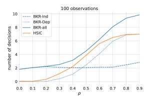
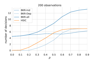
Figure 2: Synthetic dataset D1. Overall, BKR always makes more decisions than HSIC.

Figure 2(top) shows results of the comparison for a dataset D1 of $100$ observations. We have reported the number of decisions of (i) independence for BKR (BKR-Ind); (ii) dependence for BKR (BKR-Dep); (iii) overall dependence/independence for BKR (BKR-all); (iv) dependence for HSIC. BKR makes overall more decisions than HSIC for all values of the simulated correlation $\rho$. For instance for $\rho=0.9$, BKR makes $\sim 10$ decisions and HSIC only $7$. The reason is that HSIC can never declare independence. It can also be observed that BKR is calibrated under the null hypothesis (number of dependence decisions is zero when $\rho=0$) and moreover it can detect two independences. Dataset D2 is generated in a similar way but simulating a nonlinear dependence using a Clayton Copula (instead of a Gaussian Copula). Similar results were obtained for the Clayton Copula which are reported in the Supp. Material.

MIC.

We compare BKR against the Maximal Information Coefficient (MIC) [14]. The MIC statistic measures (in a non-parametric way) the strength of the association between two continuous variables; in principle it can detect any functional dependence between two variables. A MIC-based NHST of independence is obtained as described in [14]. For comparison, we consider the performance statistics from the 2008 Major League Baseball (MLB) season [14] (131 variables).

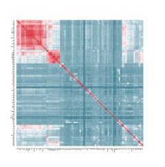
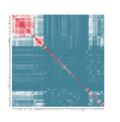
Figure 3: MLB dataset overview heatmap: red shows dependences and blue shows independences. In the left, MIC statistics. In the right, $\mathcal{E}(\text{BdCor})$. (Details of the graphs are not visible – they are intended to provide an overview picture only.)

Figure 3 shows the values of the MIC statistics and the posterior mean $\mathcal{E}(\text{BdCor})$ as a heatmap for all the $8515$ pairwise comparisons. In both cases, red denotes large values of the statistics (a sign of dependence) and blue small values (a sign of independence). The two measures provide a similar evaluation of the strength of the pairwise associations: this shows that our proposed BdCor measure is commensurable.

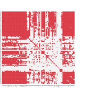
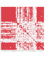
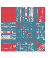
HSIC	MIC	BKR

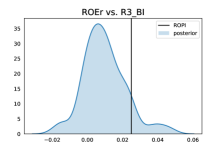
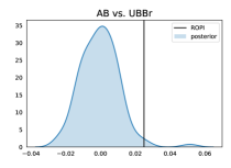
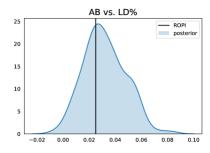
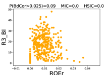
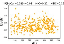
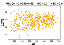
Figure 4: Left: MLB heatmap overviews showing cases where HSIC and MIC cannot discriminate statistical and practical significance. Right: Scatter and density plots for three illustrative comparisons: (i) for ROEr vs. R3BI: BKR correctly declares practical independence, while both MIC and HSIC reject independence (from the scatter plot it is evident that the dependence is overall weak); (ii) for AB vs. UBBr, MIC and HSIC cannot make any decision, while BKR declares practical independence; (iii) AB vs. LD% MIC and BKR are undecided, while HSIC rejects dependence (scatter plot shows that variables are only weakly dependent).

The NHST based on MIC cannot convert association strength analysis in assessments of independence/weak dependence. Therefore, it is not able to distinguish between statistical and practical significance. This is illustrated in Figure 4’s heatmaps where we compare the decisions of three methods. NHSTs based on HSIC and MIC detect a large set of dependencies (red), but some of them are spurious. The white colour corresponds to statistically insignificant relationships ($\alpha=0.05/8515$ with Bonferroni correction), which include relationships of independence that a NHST cannot detect. BKR is able to assess both dependence (red) and independence (blue). The scatter and density plots show the limits of NHSTs in three comparisons.

Gapminder.

The Gapminder dataset includes 319 global developmental indicators (such as education, health, trade, poverty, population growth, and mortality rates) for 200 countries spanning over 5 centuries [15]. We only consider the year 2002 and we compare three dependence detection techniques: BKR, HSIC (with Bonferroni correction), and another Bayesian approach called MI-Crosscat (the mutual information computed using Crosscat). Cross-Categorization (CrossCat) is a general Bayesian non-parametric method for learning the joint distribution over all variables in a mixed-type, high-dimensional population. In particular, the learned joint distribution can be used to perform a pairwise dependence/independence test based on the mutual information [16]. The CrossCat prior induces sparsity over the dependencies; in BKR we can induce sparsity by increasing the width of the ROPI.

Figure 5 shows the heatmap of the posterior mean $\mathcal{E}(\text{BdCor})$ computed using BKR.

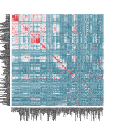
Figure 5: $\mathcal{E}(\text{BdCor})$.

This allows us to immediately capture the strength of pairwise association (red means strong, blue means weak) and to select a value for ROPI to induce sparsity. We select ROPI $0.15$ and plot the heatmap for the posterior probability of dependence (red) and independence (blue) in Figure 6(top-row).

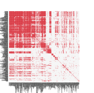
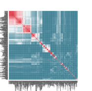
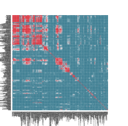
HSIC	MI-Crosscat	BKR

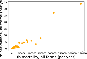
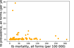
Figure 6: Gapminder dataset results.

Figure 6(top-row) shows the pairwise probability that the mutual information (MI), computed using Crosscat, exceeds zero, that is, $P[MI(X_{i},X_{j})>0]$. Note that the metric $P[MI(X_{i},X_{j})>0]$ only indicates the existence of a predictive relationship between $X_{i}$ and $X_{j}$, but it does not quantify the strength of such relationship [16]. By comparing MI-Crosscat and BKR it is evident that both Bayesian methods provide a closer insight while HSIC can only reject independence. There are also evident differences: Crosscat is not able to detect some dependences due to outliers. Consider for instance the variables A=’tb mortality, all forms (per 100 000 population)’, B=’tb prevalence, all forms (per year)’ and C=’tb mortality, all forms (per year)’: the scatter plots for (A,B) and (B,C) are showed in Figure 6. Variables are pairwise dependent and BKR assigns probability $1$ to both the comparisons, while Crosscat assigns probability $1$ for (B,C) and probability $0.04$ for (A,B) due to outliers. More examples are reported in the Supp. Material. Crosscat is a more complex and so more computationally costly model than the one used to derive BKR, but BKR offers an effective and fast way to compute dependence/independence for mixed-type variables.

Predicting classifier performance.

We have shown that BdCor is a commensurable measure of association by comparing it with MIC and MI-Crosscat. In machine learning, dependence measures are often used to assess what features are relevant for a certain prediction task. Here we use BdCor to quantify the association between all features of a dataset together ($X$) and the class variable $Y$ in 84 datasets (details in the Supp. Material) from the Penn Machine Learning Benchmarks [13]. We have used the Nyström low-rank approximation with a RBF kernel for $X$ and a indicator kernel for $Y$. For each dataset, we have also trained a logistic classifier and computed the averaged 10-fold cross-validation log-loss. Figure 7 shows the regression plot of BdCor vs. averaged log-loss: larger values for $\mathcal{E}(\text{BdCor})$ correspond to lower values for log-loss. This again confirms that $\mathcal{E}(\text{BdCor})$ is an effective measure of association.

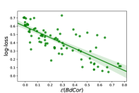
Figure 7: Predicting classifiers performance

DGT-Translation Memory.

DGT-TM is a translation memory (sentences and their manually produced translations) in 24 languages. It contains segments of all the treaties, regulations, and directives adopted by the European Union. The documents in different languages are aligned in accordance with well-defined segmentation rules. Figure 8 shows an example of the English and Italian versions of Document 52015BP0930; the rectangles bound the segments.

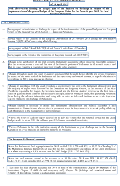
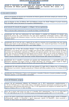
EN	IT

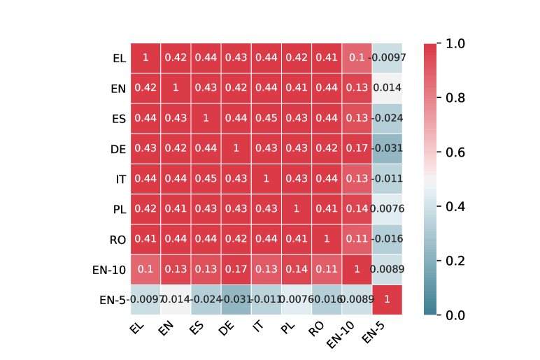
Figure 8: DGT-Translation Memory results. Two document examples (on top) and heatmap among languages.

We apply BKR to test the association between 7 different translations (’EL’,’EN’,’ES’,’DE’,’IT’,’PL’,’RO’) of the above document by considering the 18 segments in Figure 8. We have also generated two additional documents in English obtained by randomly selecting 10 (’EN-10’) and 5 (’EN-5’) words in each segment. We have used the Edit-distance-based RBF kernel. Figure 8(bottom) reports a summary of the results for all pairwise comparisons performed using BKR; each number in the heatmap cell is the posterior mean of BdCor, and the color of the cell is the posterior probability of practical dependence $p(\text{BdCor}>0.025|Data)$. BKR is able to detect the strong association among the documents. Note that Spanish (’ES’) and Italian (’IT’) have the largest value of BdCor (as expected, because of their similarity). BKR can detect dependence even using only 10 words per segment (’EN-10’). With 5 words per segment, BKR (understandably) declares weak dependence with higher probability.

6 Conclusions

We proposed a novel Bayesian kernelised association measure by using a kernel embedding of probability measures based on a Dirichlet Process prior. By using this setting, we derived a new Bayesian kernel test of independence/dependence. This test overcomes the limitations of null hypothesis significance testing (NHST) and, in particular, allows the data analyst to “accept” the null hypothesis and not only to reject it. We illustrated the effectiveness of our approach by first comparing this new test with the kernel independence test developed by [12], with a test based on the maximal information coefficient, and with a Bayesian test of independence based on the Crosscat model. We showed that our test is able to declare dependence and independence and that, for this reason, it takes more decisions than NHSTs do. An important advantage of kernel tests is that they can be applied on any (un)structured data, being for instance able to detect the dependence of passages of text and their translation or the dependence between images and text. Such flexibility opens doors for many possible usages.

Appendix A Supplementary Material

A.1 Experimental method for the House dataset

In this section we outline the methodology used to produce the pairwise heatmaps shown in Figure 1. The location counts for the House dataset are quite unbalanced (some locations have only 1 or 2 houses), so we removed all locations with less than 10 houses per location. For the remaining 462 entries, we resized the four images (frontal, kitchen, bathroom, bedroom) to $32\times 32$ pixels, converted the figures in gray-scale and tiled the four images together so that the first image goes in the top-right corner, the second image in the top-left corner, the third image in the bottom-right corner, and the final image in the bottom-left corner (we used an alphabetical order based on the filename). The final image is $64\times 64$. For BKR, we used a square exponential kernel with kernel length-scale set to the median distance between points in input space for the variables number of bedrooms, number of bathrooms, area, image and image-size, and we used the indicator function for the categorical variable location. We selected ROPI=0.025 and we sampled 1000 samples from the posterior in order to compute the quantities of interest and to plot the posterior densities.

A.2 Proofs

We briefly sketch the proofs of our results. We start by proving this lemma.

Lemma 1.

Let $X,X^{\prime}\sim P$ and $P$ have distribution $w_{0}P_{0}+\sum_{i=1}^{n}w_{i}\delta_{X_{i}}$ with $W=[w_{0},w_{1},\dots,w_{n}]^{T}\sim Dir(s,1,\dots,1)$ and $P_{0}\sim Dp(s,\nu^{*})$, then

$$E_{X,X^{\prime}}(K(X,X^{\prime}))=w_{0}^{2}\int K(x,x^{\prime})d\left(P_{0}(x)P_{0}(x^{\prime})\right)$$

$$+2\sum_{i=1}^{n}w_{0}w_{i}\int K(x,X_{i})dP_{0}(x)+\sum_{i=1}^{n}\sum_{j=1}^{n}w_{i}w_{j}K(X_{i},X_{j})$$ (13)

$$=W\mathbb{K}^{XX}W^{T}$$ (14)

where $\mathbb{K}^{XX}$ is a symmetric $(n+1)\times(n+1)$ matrix such that $\mathbb{K}^{XX}_{00}=\int K(x,x^{\prime})d(P_{0}(x)P_{0}(x^{\prime}))$, $\mathbb{K}^{XX}_{0i}=\int K(x,X_{i})dP_{0}(x)$ for $i>0$ and $\mathbb{K}^{XX}_{ij}=K(X_{i},X_{j})$ for $i=1,\dots,n$ and $j\geq i$.

Proof.

Since we have assumed that $X,X^{\prime}\sim P$, then we have that

$$E_{X,X^{\prime}}(K(X,X^{\prime}))=\int K(x,x^{\prime})d\left(P(x)P(x^{\prime})\right).$$

By exploiting $P=w_{0}P_{0}+\sum_{i=1}^{n}w_{i}\delta_{X_{i}}$, we obtain (13). The last equality (14) follows from vector algebra. ∎

Proof of Theorem 1

Theorem 1 can be obtained by Proposition 1 and Lemma 1, by noticing that, in this case, the observations are paired $Z=[X,Y]$. Under the hypothesis $X\mathbin{\mathchoice{\hbox to0.0pt{\hbox{\set@color$\displaystyle\perp$}\hss}\kern 3.46875pt{\not}\kern 3.46875pt\hbox{\set@color$\displaystyle\perp$}}{\hbox to0.0pt{\hbox{\set@color$\textstyle\perp$}\hss}\kern 3.46875pt{\not}\kern 3.46875pt\hbox{\set@color$\textstyle\perp$}}{\hbox to0.0pt{\hbox{\set@color$\scriptstyle\perp$}\hss}\kern 2.36812pt{\not}\kern 2.36812pt\hbox{\set@color$\scriptstyle\perp$}}{\hbox to0.0pt{\hbox{\set@color$\scriptscriptstyle\perp$}\hss}\kern 1.63437pt{\not}\kern 1.63437pt\hbox{\set@color$\scriptscriptstyle\perp$}}}Y$, we assume that $X,Y$ are jointly distributed with posterior distribution $w_{0}P_{0}+\sum_{i=1}^{n}w_{i}\delta_{Z_{i}}$, with $W=(w_{0},w_{1},\dots,w_{n})\sim Dir(s,1,\dots,1)$ and $P_{0}\sim Dp(s,\nu^{*})$ ∎.

An empirical estimate of the HSIC statistics from i.i.d. samples $(x_{1},y_{1}),\dots,(x_{n},y_{n})$ on $\mathcal{X}\times\mathcal{Y}$ can be obtained by replacing the expectation operators in (2) with the sample mean [12] and it is given by

$$\text{HSIC}_{obs}(X,Y) =\frac{1}{n^{2}}\sum_{i,j=1}^{n}k_{\mathcal{X}}(X_{i},X_{j})k_{\mathcal{Y}}(Y_{i},Y_{j})$$

$$+\frac{1}{n^{4}}\sum_{i,j,q,r=1}^{n}k_{\mathcal{X}}(X_{i},X_{j})k_{\mathcal{Y}}(Y_{q},Y_{r})$$

$$-\frac{2}{n^{3}}\sum_{i,j,q=1}^{n}k_{\mathcal{X}}(X_{i},X_{j})k_{\mathcal{Y}}(Y_{i},Y_{q}).$$ (15)

We now establish a connection of that with our Bayesian estimator for HSIC.

Proof of Theorem 2

We exploit the fact that for large $n$, we have that $P\approx\sum_{i=1}^{n}w_{i}\delta_{Z_{i}}$. The effect of the prior measure vanishes at the increase of $n$. Hence, we have that

$$\widehat{\text{HSIC}}(X,Y) =\sum_{i,j=1}^{n}k_{\mathcal{X}}(X_{i},X_{j})k_{\mathcal{Y}}(Y_{i},Y_{j})w_{i}w_{j}$$

$$+\sum_{i,j,q,r=1}^{n}k_{\mathcal{X}}(X_{i},X_{j})k_{\mathcal{Y}}(Y_{q},Y_{r})w_{i}w_{j}w_{q}w_{r}$$

$$-2\sum_{i,j,q=1}^{n}k_{\mathcal{X}}(X_{i},X_{j})k_{\mathcal{Y}}(Y_{i},Y_{q})w_{i}w_{j}w_{q}.$$ (16)

The moments of the Dirichlet distributions are

$$\mathcal{E}\left(w_{i}w_{j}\right)=\dfrac{1+I_{i=j}}{n(n+1)},$$

$$\mathcal{E}\left(w_{i}w_{j}w_{q}\right)=\dfrac{1+I_{i=j\vee i=q\vee j=q}+4I_{i=j=q}}{n(n+1)(n+2)},$$

$$\mathcal{E}\left(w_{i}w_{j}w_{r}w_{q}\right)=\dfrac{1+I_{i=j\vee i=q\vee j=r\vee j=r\vee j=q\vee r=q}}{n(n+1)(n+2)(n+3)}$$

$$+\dfrac{4I_{i=j=r\vee i=j=q\vee i=r=q\vee j=r=q}+18I_{i=j=r=q}}{n(n+1)(n+2)(n+3)}.$$ (17)

For large $n$, (16) converges to (15). We can recover a similar result for the variance of $\widehat{\text{HSIC}}(X,Y)$ and then use [12, Th.1 and Th.2] to prove asymptotic consistency.∎

Proof of Corollary 1

We exploit the following property of the Schur product:

$$W(K^{XX}W^{T}\circ K^{YY}W^{T})=Tr(\text{diag}(W)K^{XX}W^{T}WK^{YY}).$$

Hence, note that for $R=\text{diag}(W)-W^{T}W$,

$$Tr(K^{XX}RK^{YY}R) =Tr(K^{XX}\text{diag}(W)K^{YY}\text{diag}(W))$$

$$-2Tr(K^{XX}\text{diag}(W)K^{YY}W^{T}W)$$

$$+Tr(K^{XX}W^{T}WK^{YY}W^{T}W)$$

$$=W(K^{XX}\circ K^{YY})W^{T}$$

$$-2Tr(K^{XX}\text{diag}(W)K^{YY}W^{T}W)$$

$$+WK^{XX}W^{T}WK^{YY}W^{T}$$

$$=W(K^{XX}\circ K^{YY})W^{T}$$

$$-2W(K^{XX}W^{T}\circ K^{YY}W^{T})$$

$$+WK^{XX}W^{T}WK^{YY}W^{T}\,.$$

∎

Proof of Theorem 3

We provide the proof for the Nyström method, while the idea is similar for random Fourier features. The low-rank approximation approach provided by the Nyström method is achieved by randomly sampling $m$ data points (i.e. inducing variables) from the given $n$ samples and computing the approximate kernel matrix $\tilde{K}$:

$$\tilde{K} =K_{n,m}K_{m,m}^{-1}K_{m,n}=(K_{n,m}K_{m,m}^{-0.5})(K_{n,m}K_{m,m}^{-0.5})^{T}$$

$$=\tilde{\phi}\tilde{\phi}^{T}$$

that provides a feature representation for $\tilde{K}$. Hence, we have that

$$Tr(K^{XX}RK^{YY}R) \approx Tr(\tilde{K}^{XX}R\tilde{K}^{YY}R)$$

$$=Tr(\tilde{\phi}_{X}\tilde{\phi}_{X}^{T}R\tilde{\phi}_{Y}\tilde{\phi}_{Y}^{T}R)$$

$$=||\tilde{\phi}_{X}^{T}R\tilde{\phi}_{Y}||_{F}^{2}.$$

A.3 Pseudo-code for BKR

We provide an algorithm to perform the Bayesian non-parametric kernel test of independence ($N_{mc}$ denotes the number of Monte Carlos samples):

1. Initialise the counter $\tau$ to $0$ and the array $V$ to empty;

2. For $i=1,\dots,N_{mc}$

   1. Sample $(\omega_{0},\omega_{1},\dots,\omega_{n})\sim Dir(s,1,\dots,1)$ and $P_{0}$ from the prior Dirichlet process $Dp(s,\nu^{*})$ (via stick-breaking);

   2. Compute $\widehat{HSIC}(X,Y)$, $\widehat{HSIC}(X,X)$, and $\widehat{HSIC}(Y,Y)$ as in Equation (9);

   3. Sample a permutation $\pi$ of the list $[1,2,\dots,n]$ and compute $\tau=\tau+\widehat{HSIC}(X,Y_{\pi})/n$;

   4. Compute

      $$\widehat{HSIC}(X,Y)/\sqrt{\widehat{HSIC}(X,X)\widehat{HSIC}(Y,Y)}$$

      and store the result in $V$;

3. Compute the histogram of the elements in $\tilde{V}=(V-\tau)/(1-\tau)$ (this gives us the plot of the posterior of BdCor).

4. Compute the posterior probability that BdCor is greater than ROPI as $\mathcal{P}(\text{BdCor}>ROPI)\approx\frac{\#(\tilde{V}>ROPI)}{N_{mc}}$.

A.4 Synthetic data

Table 1 shows an instance of D1 including $n=5$ observations generated with $\rho=0.9999$.

$X$	$Y$	$C_{X}^{\rho}$	$D_{X}^{\rho}$	$D_{Y}^{\rho}$	$\mathbb{C}_{X}^{\rho}$
-0.99784	1.0	-0.99827	0.0	1.0	[0.15922, 0.15967, 0.159..]
1.25424	0.0	1.25572	1.0	0.0	[0.89481, 0.89531, 0.895…]
-0.65891	1.0	-0.65962	0.0	1.0	[0.25504, 0.25559, 0.255…]
0.08530	0.0	0.08667	1.0	0.0	[0.53422, 0.53310, 0.533…]
1.27031	0.0	1.26787	1.0	0.0	[0.89805, 0.89818, 0.898…]

Table 1: An instance of D1 for $n=5$ and $\rho=0.9999$.

Figure 9 shows the results for the simulations with Gaussian Copula with ROPI=0.05 (top) and Clayton Copula with ROPI=0.025 as discussed in Section 5.1 of the paper.

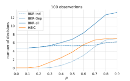
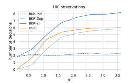
Figure 9: Synthetic dataset D1 with ROPI=0.05 and synthetic dataset D2 with ROPI=0.025

A.5 Experimental method for the MIC dataset

For BKR, we used a square exponential kernel with kernel length-scale set to the median distance between points in input space. For MIC, we have approximated the null distribution by randomly permuting one of the variables in the comparison, repeating $500$ times, and then used the approximated null distribution to compute p-values. We have used a similar approach for HSIC.

A.6 Experimental method for the Gapminder dataset

In this section we outline the methodology used to produce the pairwise heatmaps shown in Figures 5 and 6. For BKR and HSIC, for each pairwise comparison, all records in which at least one of the variables is missing were dropped. If the total number of remaining observations was less than three, the returned decision was “undecided” (p-value=0.5 and posterior probability equal to 0.5).

Figure 10 shows the scatter plots of 8 pairwise comparisons for the Gapminder datasets. The title of each plot reports the posterior probability of dependence computed by BKR (left) and Crosscat (right). Both tests agree for most of the comparisons, even though there are differences in the presence of outliers. For instance, BKR is able to detect the dependence in the last two plots, while the Crosscat probability is close to indicate independence.

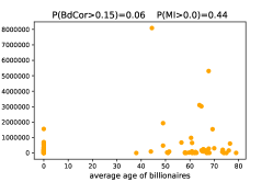
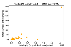
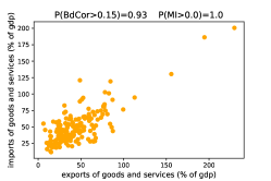
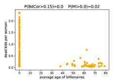
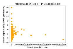
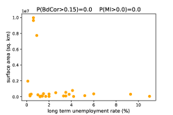
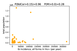
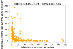
Figure 10: Gapminder dataset

	name	#instances	#features	#classes	$\mathcal{E}(BdCor)$	log-loss
0	GAM_Epi_2-Way_20atts_0.1H_EDM-1_1	1600	20	2	-0.008035	0.702575
1	GAM_Epi_2-Way_20atts_0.4H_EDM-1_1	1600	20	2	-0.007973	0.705753
2	GAM_Epi_3-Way_20atts_0.2H_EDM-1_1	1600	20	2	-0.006651	0.703142
3	GAM_Het_20atts_1600_Het_0.4_0.2_…	1600	20	2	-0.007961	0.705855
4	GAM_Het_20atts_1600_Het_0.4_0.2_…	1600	20	2	-0.007268	0.705941
5	Hill_Valley_with_noise	1212	100	2	-0.000064	0.609377
6	Hill_Valley_without_noise	1212	100	2	-0.002888	0.616655
7	analcatdata_authorship	841	70	4	0.671466	0.046860
8	australian	690	14	2	0.292128	0.329723
9	backache	180	32	2	0.049330	0.482633
10	balance-scale	625	4	3	0.309459	0.365887
11	banana	5300	2	2	0.042040	0.685723
12	biomed	209	8	2	0.271644	0.269282
13	breast	699	10	2	0.759781	0.117858
14	breast-cancer	286	9	2	0.071111	0.566539
15	breast-cancer-wisconsin	569	30	2	0.554668	0.076874
16	breast-w	699	9	2	0.769333	0.116817
17	buggyCrx	690	15	2	0.236791	0.333144
18	bupa	345	6	2	0.021190	0.620984
19	car	1728	6	4	0.070974	0.698769
20	cars	392	8	3	0.281463	0.507757
21	cars1	392	7	3	0.261504	0.561553
22	churn	5000	20	2	0.046255	0.320298
23	cleve	303	13	2	0.236671	0.445662
24	colic	368	22	2	0.133850	0.495178
25	corral	160	6	2	0.296792	0.262120
26	credit-a	690	15	2	0.237597	0.340254
27	credit-g	1000	20	2	0.028159	0.535588
28	crx	690	15	2	0.235325	0.341087
29	dermatology	366	34	6	0.749185	0.148374
30	diabetes	768	8	2	0.138120	0.480159
31	dna	3186	180	3	0.209221	0.185771
32	ecoli	327	7	5	0.642567	0.461982
33	flare	1066	10	2	0.037990	0.403444
34	german	1000	20	2	0.034654	0.530094
35	glass2	163	9	2	0.080849	0.574155
36	haberman	306	3	2	0.037010	0.559296
37	heart-c	303	13	2	0.272453	0.416660
38	heart-h	294	13	2	0.246680	0.458117
39	heart-statlog	270	13	2	0.301055	0.396709
40	hepatitis	155	19	2	0.158631	0.432231
41	horse-colic	368	22	2	0.125779	0.486803
42	house-votes-84	435	16	2	0.555361	0.141234
43	hungarian	294	13	2	0.259716	0.441491
44	ionosphere	351	34	2	0.234897	0.345410
45	irish	500	5	2	0.203002	0.488340
46	liver-disorder	345	6	2	0.021365	0.616264
47	mfeat-factors	2000	216	10	0.557608	0.148499
48	mfeat-fourier	2000	76	10	0.388237	0.560296
49	mfeat-karhunen	2000	64	10	0.448040	0.296411
50	mfeat-pixel	2000	240	10	0.525751	0.297728
51	mfeat-zernike	2000	47	10	0.409329	0.499941
52	monk1	556	6	2	0.004813	0.693910
53	monk2	601	6	2	-0.002324	0.648324
54	monk3	554	6	2	0.178117	0.391921
55	new-thyroid	215	5	3	0.521382	0.210466
56	optdigits	5620	64	10	0.530505	0.161148
57	parity5+5	1124	10	2	-0.013396	0.703223
58	phoneme	5404	5	2	0.158538	0.471846
59	pima	768	8	2	0.139403	0.494266
60	prnn_synth	250	2	2	0.335151	0.333982
61	profb	672	9	2	0.004817	0.608035
62	ring	7400	20	2	0.500697	0.521947
63	saheart	462	9	2	0.093666	0.540378
64	satimage	6435	36	6	0.580559	0.491798
65	segmentation	2310	19	7	0.571308	0.341357
66	solar-flare_2	1066	12	6	0.295000	0.729483
67	soybean	675	35	18	0.439609	0.479234
68	spect	267	22	2	0.164834	0.391502
69	spectf	349	44	2	0.161740	0.367843
70	splice	3188	60	3	0.110142	0.453967
71	texture	5500	40	11	0.461275	0.106539
72	threeOf9	512	9	2	0.127778	0.406353
73	tic-tac-toe	958	9	2	0.014250	0.628244
74	titanic	2201	3	2	0.162253	0.525138
75	tokyo1	959	44	2	0.452755	0.198396
76	twonorm	7400	20	2	0.622287	0.059936
77	vehicle	846	18	4	0.147601	0.549114
78	vote	435	16	2	0.586648	0.109903
79	waveform-21	5000	21	3	0.431121	0.311201
80	waveform-40	5000	40	3	0.382859	0.306393
81	wdbc	569	30	2	0.554726	0.075543
82	wine-recognition	178	13	3	0.660826	0.104399
83	xd6	973	9	2	0.114803	0.412084

Table 2: Predicting classifier performance using 84 datasets from the Penn Machine Learning Benchmarks repository. Last column is the log-loss of the logistic regression classifier with $L_{2}$ penalty and fixed reguralisation constant ($C=1$).

References

- [1] Eman Ahmed and Mohamed Moustafa. House price estimation from visual and textual features. arXiv preprint arXiv:1609.08399, 2016.
- [2] Nachman Aronszajn. Theory of reproducing kernels. Transactions of the American mathematical society, 68(3):337–404, 1950.
- [3] Alessio Benavoli, Giorgio Corani, Francesca Mangili, and Marco Zaffalon. A bayesian nonparametric procedure for comparing algorithms. In Proceedings of the 31th International Conference on Machine Learning (ICML 2015), pages 1–9, 2015.
- [4] Alain Berlinet and Christine Thomas-Agnan. Reproducing kernel Hilbert spaces in probability and statistics. Springer Science & Business Media, 2011.
- [5] Janez Demšar. Statistical comparisons of classifiers over multiple data sets. The Journal of Machine Learning Research, 7:1–30, 2006.
- [6] Gary Doran, Krikamol Muandet, Kun Zhang, and Bernhard Scholkopf. A permutation-based kernel conditional independence test. In the 29th Conference on Uncertainty in Artificial Intelligence (UAI), pages 132–141, 2014.
- [7] Moulines Eric, Francis R Bach, and Zaïd Harchaoui. Testing for homogeneity with kernel fisher discriminant analysis. In Advances in Neural Information Processing Systems, pages 609–616, 2008.
- [8] Thomas S. Ferguson. A Bayesian Analysis of Some Nonparametric Problems. The Annals of Statistics, 1(2):pp. 209–230, 1973.
- [9] Kenji Fukumizu, Arthur Gretton, Xiaohai Sun, and Bernhard Schölkopf. Kernel measures of conditional dependence. In Advances in neural information processing systems, pages 489–496, 2008.
- [10] Jayanta K Ghosh and RV Ramamoorthi. Bayesian nonparametrics. Springer, New York, 2003.
- [11] Arthur Gretton, Karsten M Borgwardt, Malte J Rasch, Bernhard Schölkopf, and Alexander Smola. A kernel two-sample test. Journal of Machine Learning Research, 13(Mar):723–773, 2012.
- [12] Arthur Gretton, Kenji Fukumizu, Choon H Teo, Le Song, Bernhard Schölkopf, and Alex J Smola. A kernel statistical test of independence. In Advances in neural information processing systems, pages 585–592, 2008.
- [13] Randal S. Olson, William La Cava, Patryk Orzechowski, Ryan J. Urbanowicz, and Jason H. Moore. PMLB: a large benchmark suite for machine learning evaluation and comparison. BioData Mining, 10(1):36, Dec 2017.
- [14] David N Reshef, Yakir A Reshef, Hilary K Finucane, Sharon R Grossman, Gilean McVean, Peter J Turnbaugh, Eric S Lander, Michael Mitzenmacher, and Pardis C Sabeti. Detecting novel associations in large data sets. Science, 334(6062):1518–1524, 2011.
- [15] Hans Rosling, A Rosling Ronnlund, and H Rosling. Gapminder: unveiling the beauty of statistics for a fact based world view. URL https://www. gapminder. org/data, 126, 2010.
- [16] Feras Saad and Vikash Mansinghka. Detecting Dependencies in Sparse, Multivariate Databases Using Probabilistic Programming and Non-parametric Bayes. In Aarti Singh and Jerry Zhu, editors, Proceedings of the 20th International Conference on Artificial Intelligence and Statistics, volume 54, pages 632–641. PMLR, 2017.
- [17] Dino Sejdinovic, Bharath Sriperumbudur, Arthur Gretton, and Kenji Fukumizu. Equivalence of distance-based and rkhs-based statistics in hypothesis testing. The Annals of Statistics, pages 2263–2291, 2013.
- [18] Alex Smola, Arthur Gretton, Le Song, and Bernhard Schölkopf. A hilbert space embedding for distributions. In International Conference on Algorithmic Learning Theory, pages 13–31. Springer, 2007.
- [19] Gábor J Székely and Maria L Rizzo. Brownian distance covariance. The annals of applied statistics, pages 1236–1265, 2009.
- [20] Gábor J Székely, Maria L Rizzo, Nail K Bakirov, et al. Measuring and testing dependence by correlation of distances. The annals of statistics, 35(6):2769–2794, 2007.
- [21] Gábor J. Székely and Maria L. Rizzo. The distance correlation t-test of independence in high dimension. Journal of Multivariate Analysis, 117:193 – 213, 2013.
- [22] Qinyi Zhang, Sarah Filippi, Arthur Gretton, and Dino Sejdinovic. Large-scale kernel methods for independence testing. Statistics and Computing, 28(1):113–130, 2018.