Estimating the Local Air Pollution Impacts of Maritime Traffic: A Principled Approach for Observational Data

Léo Zabrocki
Marion Leroutier
Marie-Abèle Bind

We propose a new approach to estimate the causal effects of maritime traffic when natural or policy experiments are not available. We apply this method to the case of Marseille, a large Mediterranean port city, where air pollution emitted by cruise vessels is a growing concern. Using a recent matching algorithm designed for time series data, we create hypothetical randomized experiments to estimate the change in local air pollution caused by a short-term increase in cruise traffic. We then rely on randomization inference to compute nonparametric 95% uncertainty intervals. We find that cruise vessels’ arrivals have large impacts on city-level hourly concentrations of nitrogen dioxide, particulate matter, and sulfur dioxide. At the daily level, road traffic seems however to have a much larger impact than cruise traffic. Our procedure also helps assess in a transparent manner the identification challenges specific to this type of high-frequency time series data.

Website: https://lzabrocki.github.io/cruise_air_pollution/
Replication Data: https://osf.io/v8aps/

Introduction

Maritime traffic generates economic benefits but also comes with environmental and health costs. Particulate matter pollution induced by maritime traffic was estimated to cause 60,000 premature deaths worldwide in 2007, the highest burden being born by the Mediterranean area (Corbett et al. 2007). In that region, local environmental organizations and media have recently raised increasing concerns over the potential health impacts due to air pollution emitted by cruise vessels (Friedrich 2017, Chrisafis 2018). Estimating the impact of maritime traffic on local air pollutant concentrations is however empirically challenging. Complex meteorological patterns prevail along coastal sites and influence the dispersion of air pollutants. Besides, ports are often located near major roads, making it difficult to disentangle the specific contribution of vessels to local air pollution. While atmospheric scientists can evaluate the proportion of an air pollutant concentration originating from vessel traffic, their methods are difficult to combine with counterfactual analysis preferred by economists. At the same time, in the absence of natural experiments or regulatory changes, quasi-experimental research designs are of little help to assess the effects of maritime traffic on city-level air pollution.

In this study, we propose a new approach to measure the causal effects of vessel traffic on air pollution by creating hypothetical experiments from high-frequency time series data. To illustrate our method, we focus on cruise vessel traffic in Marseille, France, which is the fourth largest Mediterranean port for cruise vessels in 2019, and a relatively polluted city by European standards. We start by combining time series data on cruise traffic, weather parameters, and air pollutant concentrations over the 2008-2018 period. By leveraging on variation in vessel traffic, we try to emulate hypothetical randomized experiments targeted for estimating the impact of a short-term increase in cruise traffic on air pollutants. To better capture the temporal chemistry of air pollutants reaction, we carry out two analyses: one at the hourly level and one at the daily level. We define treatment as hours or days with cruise vessels entering the port. Using a recent constrained pair-matching algorithm designed for time series data (Sommer et al. 2018), we construct similar pairs of treated and control time series. Contrary to propensity score matching, the algorithm we use is particularly suited to balance the lags of covariates within matched pairs, which is essential when working with time series. Once pairs are matched, we assume that the increase in cruise traffic is as-if randomized conditional on a set of observed weather parameters and calendar indicators.

Compared to an approach based on a multivariate regression model, matching has several advantages in our setting. First, it adjusts nonparametrically for observed covariates known to affect pollution in a non-linear way, such as weather parameters. Second, it helps better evaluate the initial imbalance across treated and control units: as cruise traffic has a strong seasonality, it is important to prune control units which do not belong to the common support of the data to avoid model extrapolation (King and Zeng 2006, Ho et al. 2007, Stuart 2010, Imbens 2015). Third, matching is more transparent than a regression approach to understand which observations are used as counterfactuals for treated units (Rosenbaum et al. 2010, Rosenbaum 2018).

Since our matching procedure drastically reduces the initial sample size, our preferred inference approach relies on randomization-based inference. It does not rely on large-sample approximation nor makes assumptions on the distribution of the test statistic of interest (Fisher et al. 1937, Rubin 1991, Ho and Imai 2006, Rosenbaum et al. 2010, Imbens and Rubin 2015, Dasgupta and Rubin 2021). Concretely, to quantify the uncertainty around our estimates, we build 95% Fisherian intervals that give the range of constant effects supported by the data. This mode of inference relies on the assumption of a constant unit-level treatment effect, which may not hold in our context. We therefore also quantify uncertainty using Neyman’s mode of inference (Neyman 1923), which focuses on average treatment effects, and the recent approach developed by Wu and Ding (2021) to make randomization inference asymptotically conservative when effects are heterogeneous.

Our transparent approach highlights the challenge of finding, within the time series, a suitable counterfactual for our treated units. Only 4% of treated units are matched to similar control units at the hourly level, and 8% at the daily level. This is due to fact that cruise vessel is very regular, as shown on Figure 1. Besides, up to 20% of matched pairs are temporally close from each other and might suffer from spillover effects. Despite these limits, our matching procedure is successful in creating well-balanced pairs of treated and control units.

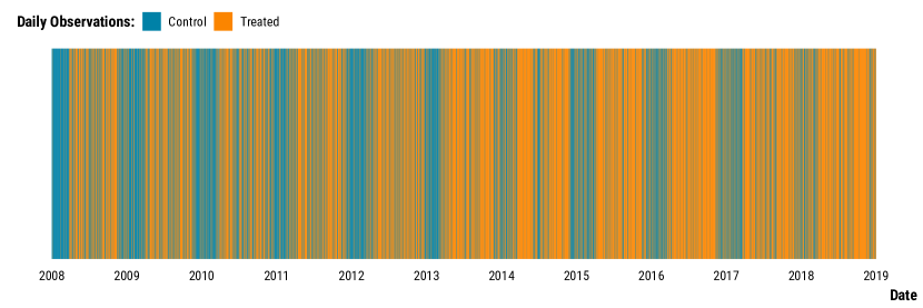
Figure 1: Regularity in Daily Cruise Vessel Traffic over the 2008-2018 Period.

Notes: Each blue line is a day without cruise traffic and each orange line is a day with cruise traffic.

At the hourly level, we find that the arrival of cruise vessel could increase nitrogen dioxide (NO₂) concentrations between 5% and 25%, coarse particulate matter (PM₁₀) between 3% and 27%, and sulfur dioxide (SO₂) between 4% and 109%. Ozone concentrations (O₃) simultaneously could decrease up to 14%, which could be consistent with the titration of this air pollutant due to an increase in nitrogen oxide (Diesch et al. 2013, Eckhardt et al. 2013, Merico et al. 2016). Contrary to hourly level results, we do not observe any clear impacts of cruise traffic on air pollution at the daily level: point estimates are null but imprecise. This lack of signal at the daily level is however consistent with a measurement campaign carried out by the local air quality monitoring agency in Marseille (Atmosud 2019). Besides, the influence of road traffic on air pollutants emitted to a large extent by cars—such as NO₂—is more discernible in the data. The higher salience of plumes emitted by cruise vessels and the potential larger concerns over this source of air pollution is an interesting area for future research. We complete our main results with an extensive set of robustness checks on issues related to unmeasured confounding, outliers, missing data and low statistical power.

Our paper contributes to the literature in several ways. First, our method is an alternative to atmospheric science methods examining contribution to air pollution by sectors. Atmospheric scientists have relied on two complementary approaches to estimate the contribution of vessel traffic to city-level pollution (Mueller et al. 2011, Piga et al. 2013, Viana et al. 2014, Liu et al. 2016, Merico et al. 2016, AtmoSud 2018, Murena et al. 2018, Liu et al. 2019, Sorte et al. 2020). The first approach is model-based. It starts by establishing an emission inventory based on vessels’ characteristics and activities. It then infers how emissions turn into concentrations using a dispersion model. The validity of this approach depends on the quality of the emission inventory and the validity of the dispersion model. The second approach is based on source apportionment methods, which require dedicated measurement campaigns with sensors deployed in the city at different seasons. The samples are then analyzed in the laboratory to detect chemical signatures and trace back the likely origin of the particles. The main limits of this second approach is that it cannot be used for gaseous pollutants and the measurement campaigns are conducted over a short period of time. Compared to these two approaches, our method tries to directly relate—without any modeling or need to analyze samples—the variation in maritime traffic to changes in the air pollutant concentrations observed at monitoring stations.

Second, our study also participates to recent works in economics examining the impact of vessel traffic on air pollution and its subsequent adverse health effects with observational data (Moretti and Neidell 2011, Zhu and Wang 2021, Hansen-Lewis and Marcus 2022, Klotz and Berazneva 2022). Several of these studies analyze the effects of fuel content regulation on air pollution, which is a convincing source of identification that can be analyzed with time-series regression discontinuity and a difference-in-difference strategies. However, many port cities around the world do not belong to emission control areas and such research designs cannot be implemented to inform future regulation policies. We instead exploit the available variation in vessels traffic to emulate hypothetical experiments. Our approach should be widely applicable to other contexts because observational data on weather, air pollution, and port call statistics are easy to access in several port cities and over a long period of time.

Third, our approach could be used as a template to help strengthen the design and analysis stages of the growing literature exploiting exogenous transport shocks to estimate the acute health effects of air pollution (Moretti and Neidell 2011, Schlenker and Walker 2016, Knittel et al. 2016, Bauernschuster et al. 2017, Zhong et al. 2017, Simeonova et al. 2021, Godzinski et al. 2019, Giaccherini et al. 2021). Matching and randomization inference have already proven to be beneficial in air pollution studies on health outcomes that do not rely on natural experiments (Baccini et al. 2017, Forastiere et al. 2020, Sommer et al. 2021, Lee et al. 2021). Even when we exploit credible source of identification, revealing the common support of the data and laying out the mode of inference is recommended in the statistics literature (Rubin 1991, Gutman et al. 2012, Zigler and Dominici 2014, Bind and Rubin 2019, Bind 2019). We clearly show in this study how matching helps evaluate the part of the data for which we can draw our inference upon since covariates balance is achieved without a parametric model. Once similar treated and control units are matched, we find more intuitive to exploit the hypothetical treatment allocation as the source of variation rather than assuming, as it is often the case, that observations have been sampled from a larger population (Abadie et al. 2020). If randomization inference has recently been the subject of a renewed interest in social sciences (Ho and Imai 2006, Cohen and Dupas 2010, Bowers and Panagopoulos 2011, Gerber and Green 2012, Athey and Imbens 2017, Heß 2017, Bowers and Leavitt 2020) and statistics (Cattaneo et al. 2015, Ding et al. 2016, Keele and Miratrix 2019, MacKinnon and Webb 2020, Caughey et al. 2021, Wu and Ding 2021, Zhao and Ding 2021), it is comparatively rather underused in environmental economics. We make great efforts to clearly explain the advantages and drawbacks of this mode of inference but also how to concretely implement it. Annotated codes and supplementary materials are available on this website. Our data are archived on a Open Science Framework repository.

The rest of our paper is organized as follows. In sections 2 and 3, we present our data and describe the research design we rely on. In section 4, we present the results and their robustness checks. In section 5, we discuss the advantages but also the limits of our approach and reflect on promising paths for future research.

Data

Figure 2: Map of Marseille’s Port surrounding Area and Hourly Vessel Traffic Variation.

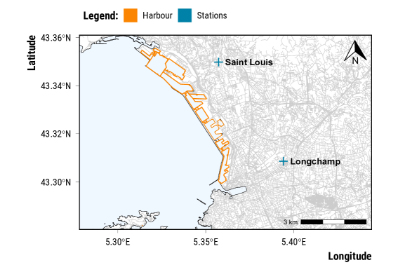
A

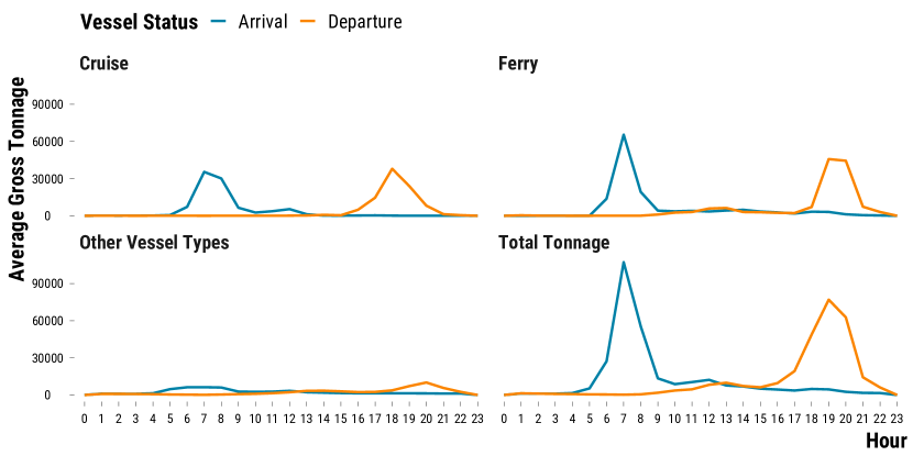
B

Notes: Panel A displays a map of Marseille city with its port and the two air quality monitoring stations located in Lonchamp and Saint-Louis neighborhoods. Grey lines represent the road network of the city. Panel B shows the average hourly variation in the gross tonnage of vessel arriving and departing the port. Gross tonnage is a unitless measure of the volume of a ship.

We built two datasets for the 2008-2018 period, one at the hourly level with 96,432 observations, and one at the daily level with 4,018 observations. Below we detail the data sources and variables used. In the Data section of our website, we report additional information on the data wrangling procedure and carry out a full exploratory data analysis (Tukey et al. 1977, Tufte 1985, Cleveland 1993).

Vessel Traffic Data

Most of the maritime passenger traffic occurs in the part of the port located in the city centre of Marseille. This means that a large fraction of the city’s residents is potentially exposed to vessels’ emissions. This is not an unusual setting as many Mediterranean cities have a port located in the city centre due the development of their economic activities over the centuries. Furthermore, in the absence, until recently, of stringent standards on the pollution content of maritime fuels, cruise vessels entering Marseille port were only subject to the standards imposed to passengers vessels in the European Union. These standards impose a sulfur content of fuels that remains fifteen times higher than the standard in Emission Control Areas existing in Northern Europe and North America.

We obtained data on 41,015 port calls from the Marseille Port authority. They represent the universe of all port calls between 2008 and 2018. For each vessel docking at the port, we know the exact date and hour of arrival and departure, as well as its name, its type, and its gross tonnage, which is a nonlinear and unitless measure of a vessel’s overall internal volume. This measure of a vessel’s volume can be related to its emissions of air pollutants and has been used in other studies as a proxy for the intensity of vessel traffic (Contini et al. 2011, Moretti and Neidell 2011). Using information on vessel characteristics, we defined three broad categories: cruise, ferry, and other types of ships. We then calculated, for each vessel type, the total number of vessels and the sum of gross tonnage entering and leaving the port at the hourly and daily levels. As shown in the Panel B of Figure 2B, vessel traffic is regular: most vessels dock in the port in the morning and leave in the evening.

Air Pollution and Weather Data

We retrieved air pollution data from the two background monitoring stations managed by AtmoSud, the local air quality agency. The first station, Saint-Louis, is the closest to the cruise terminal. It is located two kilometers away from the cruise terminal (North-Western extremity of the port) and six kilometers away from the ferry terminal (South-Eastern extremity of the port) (See Panel A of Figure 2B). It only monitors NO₂ and PM₁₀. The second station, Longchamp, is located six kilometers away from the cruise terminal and three kilometers away from the ferry terminal (See Panel A of Figure 2B). The Longchamp station monitors NO₂, SO₂, ozone (O₃), PM_2.5 and PM₁₀. Sulphur oxides (SOx), nitrogen oxides (NOx), and fine particulate matter are emitted to the atmosphere as a direct result of the combustion of maritime fuel (Sorte et al. 2020). SOx and NOx emissions directly produce NO₂ and SO₂, and contribute to the formation of secondary pollutants such as particulate matter of a larger size (i.e., PM_2.5 and PM₁₀), and O₃ (Viana et al. 2014).

Weather data come from Météo-France, the French national meteorological service. We obtained data from the closest weather station, located 25 kilometers away from the city center, at Marseille airport. We calculated hourly and daily values for weather variables: rainfall height (mm), average temperature (°C), humidity (%), wind speed (m/s), and wind direction measured on a 360 degrees compass rose where 0° is North.

To avoid losing statistical power, we imputed missing values of cruise gross tonnage, air pollutant concentration and weather parameters. We relied on the chained random forest algorithm provided by the R package missRanger (Mayer 2019). There were no clear missingness patterns for these variables and we checked with simulation exercises that this algorithm had a relatively good performance for imputing missing values, even if it could sometimes result in large discrepancies.

Road Traffic Data

We obtained hourly data on the average flow of vehicles and road occupancy rates over the 2011-2016 period from the Direction Interdépartementale des Routes, a decentralized state administration in charge of managing, maintaining, and operating roads. We selected hourly data for the six traffic monitoring stations with the best available recordings, two located North and four located East of the city. As measures of road traffic, we focus on the hourly flow of vehicles (number of vehicles) and the occupation rate of the road (%).

Research Design

We conceptualize plausible but hypothetical randomized experiments to estimate the short-term effects of an increase in vessel traffic on air pollutant concentrations in Marseille. We follow a causal inference pipeline conceived to analyze observational data in a rigorous and transparent manner (Rubin 2008, Rosenbaum et al. 2010, Bind and Rubin 2019, Sommer et al. 2021).

Stage 1: Formulating Plausible Interventions on Vessel Traffic

We are interested in the following causal question: Does cruise vessel traffic contribute to background air pollutant concentrations in Marseille? The “ideal" experiment would randomly allocate hours or days to high versus low cruise vessel traffic. We could then confidently attribute the resulting differences in pollutant concentrations to vessel emissions. In the absence of such randomized experiment in Marseille, we try to approximate an experimental setting by comparing pairs of short time series that are as similar as possible on a set of observed covariates but differ in their level of vessel traffic. We define below our hypothetical randomized experiments using the framework of the Neyman-Rubin Causal Model (Rubin 1974, Holland 1986, Rubin 2005). We conceive two hypothetical experiments: one experiment at the hourly level to test if an increase in cruise traffic affects hourly air pollutant concentrations in the very short-run; and one experiment at the daily level to examine if an increase in cruise traffic affects daily average concentrations.

The units, which we index by t (t = 1, …, T), are either hours or days spanning over the 2008-2018 period, depending on the time scale of the experiment considered. At the hourly level, $V_{t}$ is the sum of the gross tonnage of cruise vessels docking in the port during hour t. We focus on the pollution impact of cruise vessels arriving in the port rather than aggregating arrivals and departures, because the pollution impact of traffic is likely to depend on the direction of the flow. For example, cruise vessels entering the port may take time to finish maneuvering and generate emissions while they are docked. In contrast, cruise vessels leaving the port may start running their engines a few hours before effectively leaving, and therefore generate pollution over a long period of time. Here, we focus on cruise vessels’ arrivals. Our treatment indicator is $W_{t}$ and takes two values:

$$W_{t}=\begin{cases}1&\text{if $V_{t}>0$}\\ 0&\text{if $V_{t}$=0}\end{cases}$$ (1)

Hourly units with $W_{t}$ equal to one are considered as “treated" while units with $W_{t}$ equal to zero belong to the control group. A treated hour is an hour with some cruise vessel arrivals—in practice, no more than two vessels enter the port at a given hour, and more often there is only one. A control hour is an hour with no cruise vessel arriving.

At the daily level, we create a hypothetical randomized experiment easily understandable from a policy point of view. We define $N_{t}$ as the number of cruise vessels entering Marseille port on day t. Our treatment indicator is $W_{t}$ and takes two values:

$$W_{t}=\begin{cases}1&\text{if N${}_{t}=1$}\\ 0&\text{if N${}_{t}$=0}\end{cases}$$ (2)

Daily units with W_t equal to one are considered as “treated" while units with W_t equal to zero belong to the control group. A treated day is a day with one cruise vessel arriving at the port. A control day is a day without any cruise vessel arriving. On average, there is around one cruise vessel entering the port each day in the initial sample. Therefore, the results of this hypothetical experiment can be interpreted as reflecting the contribution of cruise vessel traffic on an average day of the year.

Both experiments should be seen as independent from each other, as they aim at testing the pollution impact of cruise traffic at two different time frames. Whether the impact should be stronger for specific air pollutants at the hourly or daily level is ambiguous: a measurement campaign conducted near Marseille port detected an increase in hourly concentrations of pollution consistent with maritime traffic – although they do not use vessel traffic data – but failed to detect an effect at the daily level (Atmosud 2019). It could still be argued that cruise traffic may also impact daily concentrations due to secondary pollutants taking time to form.

In our setting, each hourly and daily unit has two continuous potential outcomes whose values range in the set of plausible pollutant concentrations in $\mathrm{\SIUnitSymbolMicro g}\text{/}{\mathrm{m}}^{3}$, Y_t(0) if W_t=0 and Y_t(1) if W_t=1. As explained in the following section, our matching algorithm approximates a pairwise randomized experiment by finding similar pairs of short-time series. To properly identify a causal effect with time series data, several assumptions are required. First, we should check that pairs are well-balanced in terms of interventions occurring in the pre-treatment period. Second, we should make the Stable Unit Treatment Value Assumption (STUVA) plausible (Rubin 1974, Imbens 2015, Baccini et al. 2017, Forastiere et al. 2020). In the context of our hypothetical experiments, there must be no spillovers effects within and across matched pairs. Within a matched pair, a treated unit should be temporally far away from a control unit. Across pairs, the first lead outcome of a treated unit in one pair should not be used a control in another pair. This assumption could be harder to make for the hourly experiment since we do not have clear priors on when the treatment would actually occur. For instance, during the maneuvering phase, cruise vessels could already impact air pollutant concentrations before being docked. Once they are docked, they keep their engines on and could emit air pollution in the following hours. In the time series of the treated unit, it is therefore difficult to precisely define which lags and leads of the concentration of an air pollutant is not affected by vessel emission.

Stage 2: Designing the Hypothetical Randomized Experiments

At the design stage, our goal is to obtain a sample of similar units for which the assignment to the treatment and control groups can be assumed to be unconfounded (Rubin 1991). Formally, this unconfoundedness assumption states that the assignment to treatment is independent from the potential outcomes given a set of observed confounders. Instead of adjusting for confounding variables with a multivariate regression model, we use a novel pair-matching algorithm to obtain treated and control units with similar values for observed covariates (Sommer et al. 2021). Matching is a nonparametric method which prunes the observations to limit the imbalance between treated and control units (Ho et al. 2007, Rubin 2006, Stuart 2010, Imbens 2015). By revealing the common support available in the data, matching avoids the statistical model to extrapolate to units without empirical counterfactual.

Concretely, let X_t be the vector of observed covariates for each unit, with t the time indicator and X${}^{(k)}_{t}$ the k^th covariate. Our algorithm matches a treated unit to a control unit only if the component-wise distances between their covariate vectors (X${}^{(1)}_{t}$, X${}^{(2)}_{t}$, …, X${}^{(K)}_{t}$) are lower than pre-defined thresholds ($\delta_{1}$, $\delta_{2}$, …, $\delta_{K}$). For a pair of covariate vectors X_t and X${}_{t^{\prime}}$, we use the following distance:

$$\Delta_{\textbf{X}_{t},\textbf{X}_{t^{\prime}}}=\begin{cases}0&\text{if $\lvert X^{(k)}_{t}-X^{(k)}_{t^{\prime}}\lvert<\delta_{k}$ for all k}\\ +\infty&\text{otherwise}\end{cases}$$ (3)

Compared to a propensity score approach, we can make sure with this algorithm that observed confounders and their lags are balanced within pairs (Greifer and Stuart 2021). To limit confounding, we select two sets of covariates. First, calendar variables (i.e., hour of the day, day of the week, bank day, holidays, month, and year) are related to both vessel traffic and air pollution. Second, weather covariates (i.e., average temperature, rainfall indicator, average humidity, wind direction blowing either from the East or West, and wind speed) could also influence both vessel traffic and air pollution. We use lags of these variables to ensure that treated and control units are as similar as possible before the treatment occurs. We define matching thresholds noting that they should be strict enough to make treated and control units comparable with each other, but not too strict to avoid reducing the sample size too much. Given this trade-off, the thresholds are stricter for the hourly experiment for which the sample size is 24 times larger. Table 1 displays all threshold values used in our matching procedure.

At the hourly level, we match exactly on calendar variables (hour of the day, day of the week, bank days, holidays) over the current and two previous hours before the treatment occurred (i.e., 0, 1, 2 lags) and allow a maximum distance of 30 days between treated and control units. For weather parameters, we carried out an iterative process, for which we tried different discrepancy values and kept the ones that led to balanced treated and control groups while resulting in enough matched pairs. We found that a maximum discrepancy of around half a standard deviation often yields a good balance. We match exactly for the East and West wind directions because they play an important role in the dispersion of air pollutants.

At the daily level, we create similar pairs of treated and control units over the current and previous day before the treatment occurred (i.e., 0 and 1 lags). We relax some of the constraints from the hourly level to have enough matched pairs. We strictly match on the day of the week, bank days, and holidays over the two days of the series. We allow treated and control units to have up to three years of difference, but they should belong to the same month. For weather parameters, we match exactly on the rainfall indicator and the wind direction on days t and t-1, and we allow a small discrepancy threshold for temperature and wind speed on t and t-1.

Based on these thresholds, each treated unit is matched to its closest control unit using a maximum bipartite matching algorithm (Micali and Vazirani 1980). If no control unit is available to match a treated unit, it is discarded. We thus approximate the design of a pairwise randomized experiment where the assignment mechanism is a Bernoulli trial with a treatment probability of 0.5. Given this design, for each hypothetical experiment, the number of possible permutations is 2^P, with $P$ being the number of matched pairs.

Table 1: Maximum Discrepancies allowed for each Covariate between Treated and Control Units, Hourly and Daily Experiments.

	Hourly Experiment	Daily Experiment
Calendar Indicators
Distance in days	30	1095
Hour of the day in t	0
Weekday, Bank Days and Holidays in t	0	0
Weekday, Bank Days and Holidays in t-1	0	0
Weekday, Bank Days and Holidays in t-2	0
Month in t		0
Weather Parameters
Average Temperature (°C) in t	4	4
Average Temperature (°C) in t-1	4	4
Average Temperature (°C) in t-2	4
Rainfall Dummy in t	0	0
Rainfall Dummy in t-1	0	0
Rainfall Dummy in t-2	0
Average Humidity (%) in t	9
Average Humidy (%) in t-1	9
Average Humidity (%) in t-2	9
Wind direction in 2 categories (East/West) t	0	0
Wind direction in 2 categories (East/West) t-1	0	0
Wind direction in 2 categories (East/West) t-2	0
Wind speed (m/s) in t	1.8	2
Wind speed (m/s) in t-1	1.8	2
Wind speed (m/s) in t-2	1.8

• Notes: This table displays the maximum distance allowed for each covariate in the pair matching algorithm, for each experiment. For example, it means that, for each matched pair, treated and control units must have the same values for weekday, bank days and holidays indicators in t. If a discrepancy value is missing in one of the two column, it means that the associated covariate was not used for matching for the corresponding experiment.

Stage 3: Analyzing the Experiments using Randomization-based Inference

Once we obtain a balance sample of matched pairs, we implement a randomization-based inference procedure to analyze the effects of cruise vessels on air pollutant concentrations. Given that we have a low number of matched pairs, we rely on this particular mode of inference since it avoids large-sample approximation and is distribution-free. The hypothetical random allocation of the treatment in the matched samples is the only source of uncertainty for inference.

Point estimate for the unit-level treatment effect size.

We assume a constant additive unit-level treatment effect $\tau$:

$$Y_{t}(1)=Y_{t}(0)+\tau\text{ }\forall t=1,\ldots,\textit{T}$$ (4)

Under such assumption, the average pair difference in pollutant concentrations across treated and control units is an unbiased estimator for $\tau$ (Keele et al. 2012). Thus, for an experiment with $I_{\mathrm{Pairs}}$ matched pairs, where $Y_{1,i}^{\mathrm{obs}}$ is the observed pollutant concentration for the treated unit of pair $i$ and $Y_{0,i}^{\mathrm{obs}}$ is the observed pollutant concentration for the control unit of pair $i$, we take as a point estimate the observed value of the average pair differences:

$$\hat{\tau}=\frac{1}{I_{\mathrm{Pairs}}}\sum_{i=1}^{N_{\mathrm{Pairs}}}(Y_{1,i}^{\mathrm{obs}}-Y_{0,i}^{\mathrm{obs}})$$ (5)

Randomization-based quantification of uncertainty.

We carry out a test-inversion procedure to build 95% Fisherian (also called “Fiducial") Intervals (FI) for the constant unit-level treatment effect. We closely follow the procedure detailed by T. Dasgupta and D.B. Rubin in their forthcoming book (Dasgupta and Rubin 2021). On our website, we provide a detailed toy example to explain this mode of inference. Instead of gauging a null effect for all units, we test J sharp null hypotheses $H_{0}^{j}$: Y_t(1) = Y_t(0) + $\tau_{j}$ for j =1,$\ldots$, J, where $\tau_{j}$ represents a constant unit-level treatment effect size. We test a sequence of sharp null hypotheses of constant treatment effects ranging from -10 $\mathrm{\SIUnitSymbolMicro g}\text{/}{\mathrm{m}}^{3}$ to +10 $\mathrm{\SIUnitSymbolMicro g}\text{/}{\mathrm{m}}^{3}$ with an increment of 0.1 $\mathrm{\SIUnitSymbolMicro g}\text{/}{\mathrm{m}}^{3}$. As a test-statistic, we use the sample average of pair differences, which is commonly used in randomization-based inference (Keele et al. 2012, Imbens and Rubin 2015). For each constant treatment effect j, we calculate the upper p-value associated with the hypothesis $H_{0}^{j}$: Y_t(1) - Y_t(0) $>$ $\tau_{j}$ and the lower p-value for $H_{0}^{j}$: Y_t(1) - Y_t(0) $<$ $\tau_{j}$. We run 10,000 permutations for each hypothesis to approximate the null distribution of the test statistic. Running the exact number of possible allocations is computationally too intensive given the number of matched pairs we found. The results of testing the sequence of J hypotheses $H_{0}^{j}$: Y_t(1) - Y_t(0) $>$ $\tau_{j}$ forms an upper p-value function of $\tau$, $p^{+}(\tau)$, while the sequence of alternative hypotheses $H_{0}^{j}$: Y_t(1) - Y_t(0) $<$ $\tau_{j}$ makes a lower p-value function of $\tau$, $p^{-}(\tau)$. To calculate the bounds of the 100(1-$\alpha$)% Fisherian interval, we solve $p^{+}(\tau)=\frac{\alpha}{2}$ for $\tau$ to get the lower limit and $p^{-}(\tau)=\frac{\alpha}{2}$ for the upper limit. We set our $\alpha$ significance level to 0.05, and thus calculate two-sided 95% Fisherian intervals. This procedure allows us to get the range of constant treatment effects consistent with our data and with the hypothetical assignment mechanism we posit (Rosenbaum et al. 2010, Dasgupta and Rubin Fall 2015).

One limit of randomization inference is that it assumes a constant treatment effect across units. In our study, this is probably an unrealistic assumption: for example, we expect weather conditions to affect the relationship between cruise traffic and pollution concentration. To overcome this limit, we implement two other inference procedures that are designed for heterogeneous treatment effects. First, we can compare the results of the randomization inference procedure with the ones we would obtain with Neyman’s approach (Neyman 1923). In that case, the inference procedure is built to target the average causal effect and the source of inference is both the randomization of the treatment and the sampling from a population. We can estimate the finite sample average effect, $\tau_{\text{fs}}$, with the average of observed pair differences $\hat{\tau}$, defined as:

$$\hat{\tau}=\frac{1}{I}\sum_{i=1}^{I}(Y^{\text{obs}}_{\text{t},i}-Y^{\text{obs}}_{\text{c},i})=\overline{Y}^{\text{obs}}_{\text{t}}-\overline{Y}^{\text{obs}}_{\text{c}}$$

Here, the subscripts $t$ and $c$ respectively indicate if the unit in a given pair is treated or control. $I$ is the number of pairs. Since there are only one treated and one control unit within each pair, the standard estimate for the sampling variance of the average of pair differences is not defined. We can however compute a conservative estimate of the variance, as explained in chapter 10 of Imbens and Rubin (2015):

$$\hat{\mathbb{V}}(\hat{\tau})=\frac{1}{I(I-1)}\sum_{I=1}^{I}(Y^{\text{obs}}_{\text{t},i}-Y^{\text{obs}}_{\text{c},i}-\hat{\tau})^{2}$$

We finally compute an asymptotic 95% confidence interval using a Gaussian distribution approximation:

$$\text{CI}_{0.95}(\tau_{\text{fs}})=\Big{(}\hat{\tau}-1.96\times\sqrt{\hat{\mathbb{V}}(\hat{\tau})},\;\hat{\tau}+1.96\times\sqrt{\hat{\mathbb{V}}(\hat{\tau})}\Big{)}$$

Second, we implement the randomized inference approach recently developed by Wu and Ding (2021) that is asymptotically conservative heterogeneous effects. The procedure follows exactly the same steps previously described but is based on a studentized test statistic that is equal to the observed average of pair differences divided by Neyman’s standard error of a pairwise experiment.

Results

In this section, we first present covariate balance diagnostics on the performance of our matching procedure. We then display and interpret the results for the effects of hourly and daily cruise vessel traffic on air pollutant concentrations. We end the section with a set of robustness checks.

Matching Results

Table 2: Number of Matched Pairs by Experiment.

	Hourly Cruise Experiment	Daily Cruise Experiment
NTotal	96,432	4,018
NTreated	4,034	2,485
NControl	92,396	1,532
NPairs	138	189

• Notes: This table displays the total number of observations, N_Total for each experiment, the number of potential treated and controls units before matching, N_Treated and N_Control, and the number of matched pairs, N_Pairs.

Hourly matching diagnostics.

As shown in Table 2, our matching procedure at the hourly level results in few matched treated units, with less than 4% of treated units matched to similar control units. Two main reasons explain this result. First, cruise vessel traffic is regular over time, so that it is hard to find similar control and treated hours which are not temporally too far away from each other. Second, even if we relax our matching constraints, it is difficult to find treated and control units with similar weather covariates. We check that within pairs spillovers are not likely to occur since within a pair, treated and control units are at least 7 days away. However, there could be spillovers across pairs. For instance, for 16% of treated units, the minimum distance with a control unit in another pair is inferior or equal to 5 hours. Dropping these pairs or modifying the matching algorithm to avoid having pairs too close temporally of each others would be required to avoid spillover effects.

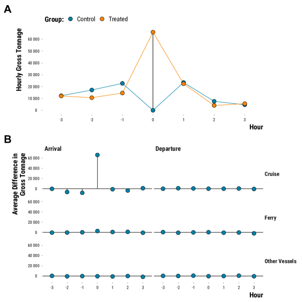
Figure 3: Intervention Diagnostics for the Hourly Experiment.

Notes: Panel A shows the average hourly total gross tonnage for matched treated and control units. Panel B plots the average difference in total gross tonnage between treated and control units by vessel type and flow.

In Figure 3, Panel A displays the average increase in cruise vessel arrivals at hour 0. The average difference in gross tonnage between treated and control units is about 65,000 for the hourly cruise experiment, which is the average gross tonnage of one cruise vessel. Panel B shows that, on average, treated and control units have similar vessel traffic for other vessel types and flows. The matching procedure at the hourly level improves the overall balance of covariates as shown in Figure 4. Further diagnostics on covariates balance are available at the hourly level on our website.

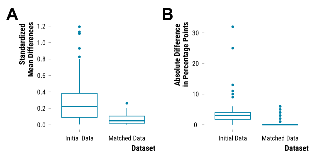
Figure 4: Improvement in Covariates Balance for the Hourly Experiment.

Notes: Panel A shows the boxplot distribution of the absolute standardized mean differences in continuous covariates before and after matching. Panel B shows the boxplot distribution of the absolute mean differences in categorical covariates before and after matching.

Finally, we compare the matched data to the initial data. Matched hours are more likely to fall on spring and summer days, which are hotter on average. They fall disproportionately around 7 am, the time where cruise vessels tend to arrive in Marseille port. All comparisons are available on our website.

Daily matching diagnostics.

At the daily level, we found 189 matched pairs, which means that 8% of the treated units were matched to similar control units. There should not be within pair spillovers since treated and control units are at least 7 days away. However, as in the hourly experiment, there could be spillovers across pairs if cruise vessel emissions impact the first lead of air pollutant concentrations. For 22% of treated units, the minimum distance with a control unit in another pair is equal to one day.

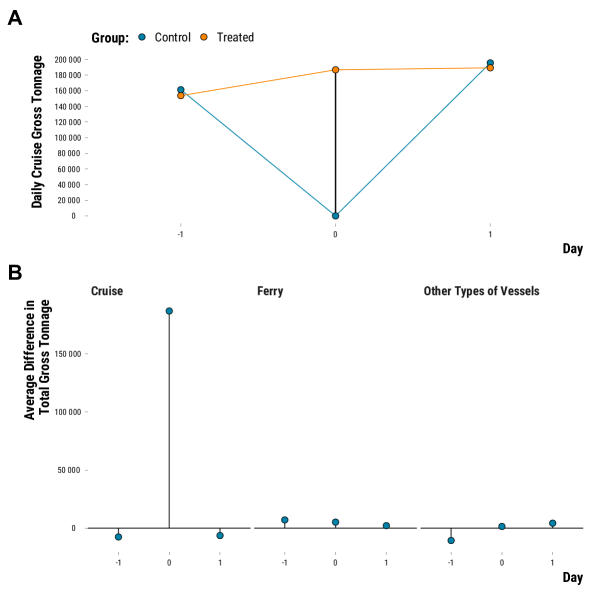
Figure 5: Intervention Diagnostics for the Daily Experiment.

Notes: Panel A shows the average daily total gross tonnage for matched treated and control units. Panel B plots the average difference in total gross tonnage between treated and control units by vessel type and flow.

In Panel A of Figure 5, the average difference in gross tonnage between treated and control units is around 150,000, which corresponds to the tonnage of two vessels. The cruise vessel entering the port in the morning most likely leaves the port in the evening after docking at the port during the day. The variation in gross tonnage for other vessel types is similar across treated and control units, as shown in Panel B of Figure 5. Similarly to the hourly experiment, the matching procedure improved the balance of covariates, as shown in Figure 6. Further diagnostics on covariates balance are available at the daily level on our website.

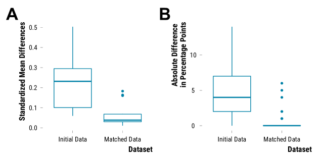
Figure 6: Improvement in Covariates Balance for the Daily Experiment.

Notes: Panel A shows the boxplot distribution of the absolute standardized mean differences in continuous covariates before and after matching. Panel B shows the boxplot distribution of the absolute mean differences in categorical covariates before and after matching.

As for the hourly experiment, days in the matched sample are more often in summer so that they are hotter, less rainy and with a lower wind speed than the average day from the initial sample. All comparisons are available on our website.

The Effects of Cruise Vessel Traffic on Air Pollutants

Hourly Effects.

In Figure 7, we plot the point estimates and the 95% Fisherian intervals of the constant treatment effects on air pollutant concentrations that are consistent with our data. We compute these effects for the three previous hours before the treatment occurs up to the three following hours in order to capture the impacts of emissions during the maneuvering phase of cruise vessels but also while they are docked with their engines on.

For NO₂, we observe an increase in concentration from the second previous hour up to the second following hour. The pattern is clearer for the Longchamp station than the Saint-Louis station where the signal is more noisy. At hour 0, concentrations are higher by 4.7 $\mathrm{\SIUnitSymbolMicro g}\text{/}{\mathrm{m}}^{3}$ (95% FI: [1.4, 8.0]). In relative terms, this represents a 16% increase in the average hourly concentration of NO₂ measured at Longchamp station. The 95% Fisherian are relatively wide since the data are consistent with constant effects ranging from a 5% increase up to a 27% increase in concentration.

For O₃, we see the opposite relationship since there seems to be a decrease in concentration in the three previous hours, followed by an increase in the following hours. In hour 0, there is a constant decrease of O₃ concentrations by 3.8 $\mathrm{\SIUnitSymbolMicro g}\text{/}{\mathrm{m}}^{3}$ (95% FI: [-7.6, 0.0]). This is equivalent to a 7% decrease in the average hourly concentration of the air pollutant. Again, the 95% Fisherian intervals are wide: the data are consistent with null effects up to a 14% decrease.

For SO₂, we observe an increase in concentrations of 1.2 $\mathrm{\SIUnitSymbolMicro g}\text{/}{\mathrm{m}}^{3}$ at hour 0 (95% FI: [-0.1, 2.5]), which persists over the two following hours. The constant increase is equivalent to a very large relative increase in concentration by 52%. The 95% Fisherian interval is also wide since the data are consistent with a relative decrease of 4% up to a relative increase of 109%.

For particulate matter, we observe an increase in PM₁₀ concentrations measured at Saint-Louis that is followed by a decrease. At hour 0, the constant increase is equal to 4.6 $\mathrm{\SIUnitSymbolMicro g}\text{/}{\mathrm{m}}^{3}$ (95% FI: [0.9, 8.3]). This is equivalent to a 15%: the data are consistent with relative increase from 3% up to 27%. There are no very clear patterns for PM₁₀ and PM_2.5 concentrations measured at Longchamp station.

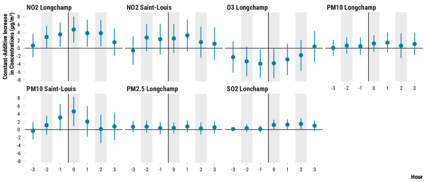
Figure 7: Effects of Cruise Vessel Traffic on Pollutant Concentrations at the Hourly Level.

Notes: The treatment occurs at hour 0. Dots represent the point estimate of the unit-level treatment effect on a pollutant concentration. Lines are 95% Fisherian intervals of constant treatment effects consistent with the data. The effects are plotted from the third lag to the third lead.

Daily Effects.

Figure 8 shows the results for the daily experiment. We can see point estimates are nearly null for all air pollutants. The 95% Fisherian intervals are however however relatively large. For instance, if the point estimate for the constant effect on NO₂ in Longchamp is nearly null, the data are consistent with effects ranging from a 6% decrease up to a 5% increase.

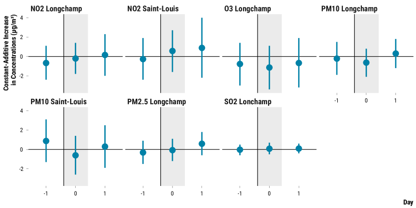
Figure 8: Effects of Cruise Vessel Traffic on Pollutant Concentrations at the Daily Level.

Notes: The treatment occurs at day 0. Dots represent the point estimate of the unit-level treatment effect on a pollutant concentration. Lines are 95% Fisherian intervals of constant treatment effects consistent with the data. The effects are plotted from the first lag to the first lead.

Neyman’s approach and randomization inference for average treatment effects.

For the hourly and daily experiments, the 95% Fisherian intervals for constant treatment effects are very similar to the intervals for the average treatment effects computed with Neyman’s approach (see Figure A.1. They are also very similar to those found with the studentized randomization inference that is conservative for weak null hypotheses (see Figure A.2. With these two alternative mode of inference, we can also confidently interpret the previous 95% Fisherian intervals as the range of average treatment effects consistent with the data.

Heterogeneity Analysis.

We carry out two heterogeneity analyses for the hourly and daily experiments. First, depending on the wind direction, the effects of cruise vessel emissions on air pollutant concentrations are likely to be attenuated or increased. At the hourly level, we observe stronger differences in concentrations for all air pollutant when the wind is blowing from the West, that is to say when vessel emissions are more likely to spread over the city (see Figure A.3). At the daily level, there are no clear patterns. Second, we also visually explore the relationship between pair differences in air pollutant concentrations against the pair differences in gross tonnage. Ideally, we should see a positive relationship since the higher the pair difference in gross tonnage (i.e., the higher the treatment shock is), the larger the pair difference in concentrations should be. We do not see any clear patterns, both for the hourly and daily experiments.

Robustness checks

We carry out several robustness checks to evaluate different aspects of the design and results of our study.

Randomization check for overall balance.

During the matching procedure, we assess the balance with Love plots that display for each covariate the standardized difference in means between treated and control units before and after matching. To better assess the overall balance, we implement the randomization inference method developed by Branson (2021) to evaluate if the treatment indicator is as-if randomized according the pairwise structure in the matched data. As a test statistic, Branson (2021) proposes to use the Mahalanobis distance which summarizes the imbalance in the means of all covariates but also takes into account their joint relationships. The randomization inference procedure consists in permuting the treatment indicator many times, computing the Mahalanobis distance for each iteration and plotting the resulting null distribution of the test statistic. If the observed value of the Mahalanobis distance is far away from the distribution, it means that the treatment is not as-if randomized according to observed covariates. For both the hourly and daily experiments, we find clear evidence that the treatment is randomized according to a pairwise structure.

Sensitivity to hidden bias.

The causal interpretation of our results is based on the plausibility of the hypothetical experiment and the unconfoundedness assumption (Rubin 1991). This is a strong assumption as it states that the treatment assignment probability is not a function of potential outcomes given observed and unobserved counfounding factors (Sekhon 2009). To evaluate the consequence of hidden bias, we rely on the sensitivity analysis framework developed by (Rosenbaum 1987, Rosenbaum et al. 2010). The goal of this method is to quantify how the treatment estimates would be altered by the effect of an unobserved confounder on the treatment odds, denoted by $\Gamma$. In our matched pairwise experiments, we make the assumption that within each pair, control and treated units have the same probability of 0.5 to be treated, that is to say to have a positive shock on cruise traffic. The odds of treatment is such that $\Gamma=(0.5/(1-0.5))/(0.5/(1-0.5))=1$. As explained in Rosenbaum et al. (2010), we can implement a randomization inference procedure to compute the 95% Fisherian intervals obtained for a given value of bias that the unmeasured confounder has on the treatment assignment. For instance, if we assume that an unmeasured confounder has a small effect on the odds of treatment (i.e., for a $\Gamma$ > 1 and close to 1) but the resulting 95% Fisherian interval is consistent with negative, null and positive effects, it would imply that our results are highly sensitive to hidden bias. Conversely, if we assume that an unmeasured confounder has a strong effect on the odds of treatment (i.e., for a large $\Gamma$) and we find that the resulting 95% Fisherian interval remains similar, it would strength our view that our results do not suffer from hidden bias. Again, the method of Rosenbaum et al. (2010) relies on the assumption of constant additive treatment effects, which is unrealistic in our study. To overcome this limit, we implement the new method proposed by Fogarty (2020) which extends the sensitivity analysis for sample average treatment effects. In a complementary evaluation of hidden bias, we also check whether unmeasured biases could be present by using the lags of air pollutant concentrations as placebo/control outcomes (Imbens and Rubin 2015). If our matched pairs are indeed similar in terms of unobserved covariates, the treatment occurring in $t$ should not influence concentration of air pollutants in the first lag at the daily level and concentrations for further lags at the hourly level.

Our sensitivity analysis reveals that the estimated effects of cruise vessels emissions on NO₂ concentrations at Longchamp station and PM₁₀ concentrations at Saint-Louis station could be affected by a relatively weak hidden bias. Concretely, if we fail in our matching procedure to adjust for an unobserved confounder which is 1.5 times more common among treated units, the resulting 95% Fisherian interval for the effects on NO₂ ranges from -1.5 $\mathrm{\SIUnitSymbolMicro g}\text{/}{\mathrm{m}}^{3}$ to 11.4 $\mathrm{\SIUnitSymbolMicro g}\text{/}{\mathrm{m}}^{3}$ and the intervals for the effects on PM₁₀ ranges from -1.9 $\mathrm{\SIUnitSymbolMicro g}\text{/}{\mathrm{m}}^{3}$ to 12.2 $\mathrm{\SIUnitSymbolMicro g}\text{/}{\mathrm{m}}^{3}$. Our data would be still consistent with mostly positive effects of cruise vessel emissions on these two air pollutants but they could be null and even negative. It is however hard to think about an unobserved confounder which would change the odds of treatment by 50%. To complement this sensitivity analysis, we also note that there are no differences in the first lag of air pollutant concentrations for the daily experiment. For the hourly experiment, we also see that for further lags and leads, estimated differences in air pollutant concentration are mostly null.

Sensitivity of results to outliers and missing observations.

In the matched data, the observed concentration of air pollutants are sometimes very high. To make sure that our results are not influenced by outliers, we run again our randomization inference procedure with the Wilcoxon signed-rank statistic. The 95% Fisherian intervals obtained with this test statistic are similar to those obtained with the average of pair differences (see hourly and daily results). Besides, we imputed missing values and we could fear that their imputations affect the results. For instance, at the hourly, up to 25% of the pairs have missing values for an air pollutant. Our simulation exercise also shows that large imputation errors sometimes occur. We therefore run again our randomization inference procedure for pairs with observed air pollutant concentrations: we find similar results with slightly wider 95% Fisherian intervals (see hourly and daily results).

Indirect treatment effect of cruise traffic.

One issue of our design could be the presence of an indirect treatment effect due to the increase in road traffic induced by cruise vessel passengers and its subsequent effects on air pollution. This is part of the causal effect that we want to capture but it is not the proper causal effect of cruise vessel emissions. We therefore check if road traffic measures are balanced before and after the treatment occurs For the hourly and daily experiments, we observe that road traffic flow and road occupancy rate appear relatively balanced across treated and control units in the matched samples of the two experiments (see hourly balance checks and daily balance checks). It is the case before and after the treatment occurs: when we observe an increase in air pollutant concentrations, this is unlikely to be due to an increase in road traffic.

Low statistical power and inflation of statistically significant estimates.

In the hourly and daily experiments, our matching procedure resulted in few matched pairs, which decreases the precision of our treatment effect estimates. Moreover, if our statistical power is low and we obtain a "statistically significant" effect, we have a higher chance that this estimate is of the wrong sign (Type S error) and overestimates the true effect of vessel traffic on air pollutant concentrations (Type M error) (Gelman and Carlin 2014, Gelman et al. 2020). We therefore carry out retrospective power calculations to evaluate the risks of making type-S and type-M errors. While it is impossible to know what the true effect of cruise vessels on an air pollutant is, we can calculate the statistical power and the risks to make type S and M errors under a set of plausible effect sizes using the closed-form expression derived by Lu et al. (2019) and implemented in the retrodesign R package by Timm (2019).

For instance, we observe a 4.7 $\mathrm{\SIUnitSymbolMicro g}\text{/}{\mathrm{m}}^{3}$ increase in NO₂ concentrations in Longchamp due to cruise vessel arrivals. If other researchers think that this effect size is too large, we can retrospectively compute the power of our study according to a range of alternative true effect size. In Figure 9, if we assume that the true effect is equal to half the estimated effect size, that is to say +2.35 $\mathrm{\SIUnitSymbolMicro g}\text{/}{\mathrm{m}}^{3}$ (dashed line), our study would have a power of 30% and "statistically significant" estimates would be on average 1.8 times too large. However, the probability that a "statistically significant" estimate is of the opposite sign is nearly null. For other air pollutants for which 95% Fisherian intervals are wider, this risk could be high. With the few number of matched pairs found in our hypothetical experiments, there is a chance that "statistically significant" estimates could be misleading: as we did, we should rather interpret the width of the 95% Fisherian intervals.

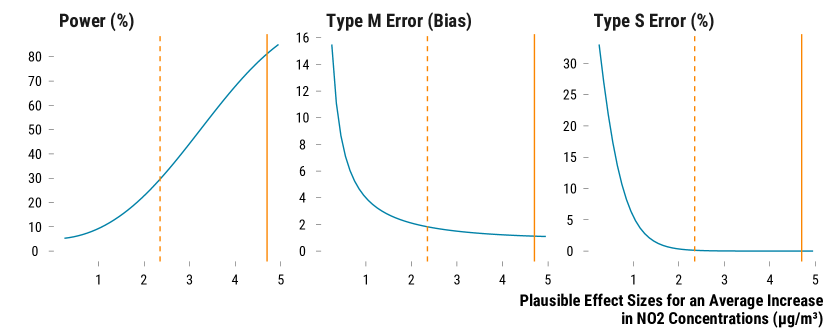
Figure 9: Statistical Power, Type M and S Errors for Hourly Experiment Effect on NO₂.

Notes: In the first left panel, the statistical power of the hourly experiment on the effect of cruise vessel on NO₂ is plotted against hypothetical true effect sizes. In the middle panel, the inflation/exaggeration ratio of statistically significant estimates is plotted against against hypothetical true effect sizes. In the right panel, the probability to get a negative statistically estimate is plotted against against hypothetical true effect sizes. The solid line is the observed estimate of the average treatment effect. The dashed line is half the value of the observed estimate.

Strictness of the matching procedure.

Our matching procedure is strict and result in a small number of matched pairs, both at the hourly and daily levels. This is partly due to the regularity in vessel traffic which makes it hard to find control units that are temporally close to treated units and with similar covariate values. To relax the stringency of our matching procedure, we implement a propensity score matching procedure where each treated unit is matched to its closest control unit if their distance is less than 0.01 of the standard deviation of the propensity score distribution. For instance, at the daily level, 1,846 pairs were matched. The Love plot indicates that covariates balance has increased but the randomization balance check suggests that the treatment is not as-if randomized according to observed covariates in the matched data. While estimates are more precise, they are relatively consistent with those found with our approach. It is very important to remind that when we compare the results of our constrained pair matching procedure with the propensity score approach, we are comparing two different subsamples of the initial dataset.

Comparison with an outcome regression approach.

Finally, we compare our results to estimates found using a simple multivariate regression model on the initial hourly and daily datasets. The matched datsets are selected sub-samples of the initial datasets and have different covariate values. Estimated effects are therefore not directly comparable. For each experiment, we run the following model:

$$p_{t+j}=\alpha+\beta W_{t}+\textbf{X}_{t}\gamma+\textbf{C}_{t}\theta+\epsilon_{t}$$

where $j$ is the index of the lag or lead, t is either the hour (for the two hourly experiment) or the day index (for the daily experiment), $p_{t+j}$ the concentration of an air pollutant $p$ at date $t+j$, $W_{t}$ the binary treatment indicator, $\textbf{X}_{t}$ the vector of weather covariates, which include the average temperature, the squared of the average temperature, an indicator for the occurrence of rainfall, the average humidity, the wind speed, the wind direction divided in the four principal directions (North-East, South-East, South-West, North-West), $\textbf{C}_{t}$ the vector of calendar variables, which are indicators for the hour of the day (for the hourly experiment), the day of the week, bank days, holidays, month, year and the interaction of these last two variables, and $\epsilon_{t}$ an error term. We run this simple model from lag 3 to lead 3 of an air pollutant for the hourly experiment on vessels’ arrivals and from lag 1 to lead 1 for the daily experiment.

At the daily level, estimates found with the regression approach are relatively similar but much more precise to those obtained with our matching procedure. However, at the hourly level, regression estimates are of smaller magnitudes and even of opposite signs for some air pollutants (see Figure 10). This could be due to the fact that we are comparing two different samples. The alternative reason to explain this discrepancy could be due the multivariate regression model failure to correctly adjust for the functional forms of confounders and to its inherent tendency to extrapolate treatment effects outside the support of the data. Hourly results on the impact of vessel emission on air pollution are also more consistent with what has been observed in previous observational studies on the impact of cruise traffic on air pollutant concentrations (Diesch et al. 2013, Eckhardt et al. 2013, Merico et al. 2016).

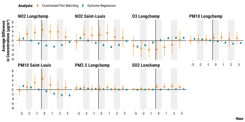
Figure 10: Comparison of Matching and Regression Results for the Hourly Experiment.

Notes: The treatment occurs at hour 0. The orange color represents the results of our matching procedure while the blue color represents results from the regression approach. Orange dots and blue triangles represent the point estimate of the average treatment effect on a pollutant concentration. Lines are 95% confidence intervals of average treatment effects consistent with the data. The effects are plotted from the third lag to the third lead.

Discussion

In this section, we start by discussing our results in view of the environmental science literature. We then reflect on the new statistical methods used for our analyses. Finally, we suggest paths for future research assessing the causal impact of maritime traffic on air pollution when natural or policy experiments are not available.

Putting our Results into Perspective

Our results point to a potential short-term effect of cruise traffic on the concentrations of NO₂, O₃, SO₂, and PM₁₀ at the hourly level. At the daily level, we do not observe an impact of cruise vessel on all air pollutant concentrations. However, for both experiments our 95% Fisherian intervals are often wide, and the implied degree of randomization-based uncertainty can be quite large relative to the average concentration of these air pollutants.

Directly comparing our results to those found in the atmospheric science literature is difficult for several reasons. First, they are based on other methods—either source apportionment techniques or dispersion modeling—and usually only report average effects without comparable measures of uncertainty. Second, they often consider the entire traffic of vessels rather than isolating the impact of a pre-defined treatment, as we do. Third, recent literature reviews have shown that the contribution of vessel emissions to local air pollution depends highly on the port-city considered and the procedure carried out by researchers (Viana et al. 2014, Murena et al. 2018). We can nonetheless assess whether our causal estimates are of the same order of magnitude as estimates from the atmospheric sciences literature.

For gaseous pollutants such as NO₂ and SO₂, the atmospheric science literature has mostly used emissions inventories combined with dispersion modeling (Viana et al. 2014). The few studies on ports from the Mediterranean area find different contributions of maritime traffic to city-level concentrations depending on the size of the city, the location of the monitoring stations, the prevailing wind patterns, the type of boat considered and the assumptions used in the emissions inventory (Murena et al. 2018, Mocerino et al. 2020). These estimates typically take into account all the phases where a vessel may contribute to pollution, in particular the hotelling phase, while we do not have information of the duration of the different phases. For NO₂, estimates range from 1.2-3.5% for the contribution of cruise ships in summer in Naples (Murena et al. 2018) to 32.5% for the contribution of all types of ships in the Italian city of Brindisi (Merico et al. 2017). Our estimated contribution of cruise traffic to NO₂ concentrations at the hourly level is equal to an increase of 16%. The estimates for SO₂ range from 1.5% for Naples in winter (Murena et al. 2018) to 46% for Brindisi in summer (Merico et al. 2017). At the hourly level, we observe an increase of 52% in SO₂ concentrations.

For particulate matter, source apportionment methods are commonly used (Sorte et al. 2020, Viana et al. 2008). Estimates for the contribution of vessels to PM₁₀ concentrations range from 1.1% for Rijeka in Croatia up to 11% for Genoa in Italy (Merico et al. 2016, Bove et al. 2014). We do not observe an effect on particulate matter in our daily experiment. This is however consistent with a measurement campaign carried out by Marseille’s air quality monitoring agency (Atmosud 2019), which relies on a five-month data collection near the port.

The media and non-governmental organizations have insisted on the high contribution of vessel traffic, and in particular cruise vessel traffic, to city-level emissions as measured by emission inventories. Our hourly experiment confirms that cruise traffic can increase air pollutant concentration on relatively short-time scale. Yet, the results of our daily experiment fail to suggest an impact of cruise vessels to air pollution on a longer time scale. We can contrast the results of our daily experiment on NO₂ concentrations with the contribution of road traffic, which can be inferred from a simple comparison between weekdays and weekends (see our simple road traffic analysis). Because they are balanced in terms of weather covariates, the difference in observed concentrations between weekdays and weekends can be attributed to differences in economic activity only, and in particular to differences in road traffic. Road traffic decreases by 20% on average on Saturdays and Sundays. In parallel, NO₂ concentrations decrease by 20% of their average level at the Saint-Louis station. Although other sources of pollution may be less intense on weekends, the road traffic and NO₂ time series follow an extremely similar pattern, suggesting a strong contribution of road traffic to ambient concentrations compared to maritime traffic. Besides, cruise traffic tends to be higher on week-end and this positive flow of vessels does not offset the likely effect of road traffic on NO₂ concentrations. Beyond emission inventories informing on the relative contribution of different sectors to emissions, more systematic assessments based on observational studies are needed to understand the relative contribution of different sources to ambient concentrations. It would help better evaluate the benefits of abatement in each sector and prioritize policies. Besides, the higher salience of plumes emitted by cruise vessels and the potential larger concerns over this source of air pollution is an interesting area for future research.

Reflection on the Methods

The causal inference pipeline we follow helps to clearly distinguish the design stage of our study—where we create hypothetical experiments—from its statistical analysis. Our pair-matching procedure has two notable advantages. First, it prunes treated units for which we cannot find a similar control unit, and thereby avoids extrapolating treatment effects for units without any empirical counterfactuals. In a way, a matching procedure reveals the common support available in the data from which we can draw our statistical inference upon. Second, our approach adjusts for covariates in a nonparametric way and achieves balance between treated and control units on observed covariates. This is another advantage, as it is often hard to guess what functional forms are needed to adjust for confounding factors (Cochran and Rubin 1973, Ho et al. 2007, Imbens 2015).

Yet, matching applied to high-frequency and regular vessel traffic data also poses difficulties. First, finding comparable treated and control units is challenging. At the hourly level, it is difficult to match a treated unit with a control unit because vessel traffic is very regular within different periods of the year. For instance, cruise vessels nearly always dock in the port at particular hours and days of the week—leaving few control hours without any cruise traffic. Second, obtaining days with close weather patterns over several consecutive days is extremely difficult: at the hourly level, it was nearly impossible to find similar pairs over three lags of covariates. Surprisingly, even if we strive to find similar pairs of treated and control units, we observe a wide heterogeneity in pair differences in pollutant concentrations, which makes it difficult to precisely estimate the potential contribution of vessel emissions. In our study, we are therefore confronted with a trade-off between the comparability of units within pairs and the sample size on which we base our statistical analysis.

Regarding the statistical inference procedure, randomization-based inference allows us to avoid large-sample approximations and makes no assumption on the distribution of our test statistic under the sharp null hypothesis (Rosenbaum et al. 2010). Given that we deal with small sample sizes, we believe that our procedure is a relevant alternative to standard quantification of uncertainty. Yet, randomization-based inference procedure relies on the stringent assumption that the treatment is constant. This is arguably an unrealistic assumption. We therefore provide results from a Neymanian inference perspective (Splawa-Neyman et al. 1990, Imbens and Rubin 2015), which considers average treatment effects rather than unit-level treatment effects. Although based on a different interpretation of the data, results from Fisherian and Neymanian inference are very similar. The recent approach proposed by Wu and Ding (2021) to make a randomization inference procedure conservative for average treatment effects also give very similar results. As an alternative to Fisherian and Neyman modes of inference, we could also have implemented a Bayesian model-based approach, which explicitly imputes the missing potential outcomes given the observed data and can target a larger variety of causal estimands (Rubin 1978, Imbens and Rubin 2015, Bind and Rubin 2019).

Finally, in terms of feasibility and data requirement, our approach could in some contexts be less costly to implement than source apportionment or dispersion modeling from the atmospheric sciences: while emission inventories and monitoring campaigns are commonplace in developed countries, they are less common in developing country contexts. In contrast, our method relies on vessel traffic data that is collected by all port authorities as part of their business activities, and can also be accessed via online platform. Pollution data from monitoring stations are often publicly available too, and could be replaced by satellite data in contexts where monitoring stations are sparse.

Potential Paths for Future Research

We see at least three main improvements for future research aiming to estimate the effects of maritime traffic on air pollution. First, it would be useful to exploit data on the duration vessels keep their engines running while docked at the port. Several studies indicate that a large share of air pollutant emissions occur during this phase (CAIMAN 2015, Murena et al. 2018). Second, monitoring stations in Marseille only measure some air pollutants and are located relatively far away from the port. It would be useful to carry out similar analyses as ours in a port city where pollutants such as ultrafine particles are monitored and with receptors located in the port at different heights (Viana et al. 2014, Mocerino et al. 2020). Besides, the weather data we exploit are located 25km away from the city, which adds noise. It would also be useful to have a monitoring station located within the city. Third, we saw that a non-negligible fraction of our matched pairs could be affected by spillover effects. New matching algorithms should be developed to force treated and control units from different pairs to be temporally far away: estimated treatment effects would be then less likely to be contaminated by spillovers.

We provide detailed replication materials in the hope that researchers could implement but also improve our method. Even if there remain challenges with regards to potential spillover effects and the imprecision of estimates, we believe that our study provides a fruitful and principled approach to try to estimate the impacts of maritime traffic on local air pollution.

Appendix A Appendix

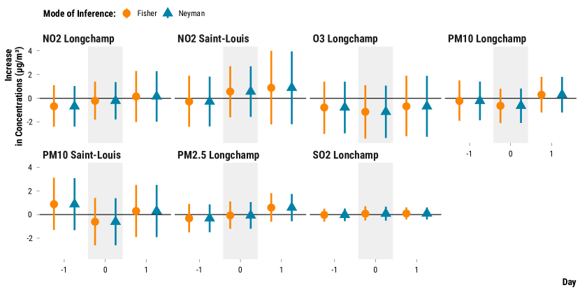
Figure A.1: Effects of Cruise Vessel Traffic on Pollutant Concentrations at the Daily Level: Comparing Fisherian and Neymanian Modes of Inference.

Notes: The treatment occurs at day 0. Dots represent the point estimate effect on a pollutant concentration. Orange lines are 95% Fisherian intervals of constant treatment effects consistent with the data. Blue lines are 95% confidence intervals based on Neyman’s mode of inference: they represent the range of average treatment effects consistent with the data. The effects are plotted from the first lag to the first lead.

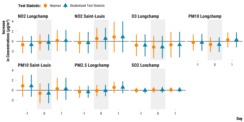
Figure A.2: Effects of Cruise Vessel Traffic on Pollutant Concentrations at the Daily Level: Comparing Neyman’s Mode of Inference to Wu and Ding (2021)’s Randomization Inference Approach for Weak Null Hypotheses.

Notes: The treatment occurs at day 0. Dots represent the point estimate effect on a pollutant concentration. Orange lines are 95% Neymanian intervals of average treatment effects consistent with the data. Blue lines are 95% Fisherian intervals based on Wu and Ding (2021)’s approach to make randomization inference asymptotically conservative for weak null hypotheses. The effects are plotted from the first lag to the first lead.

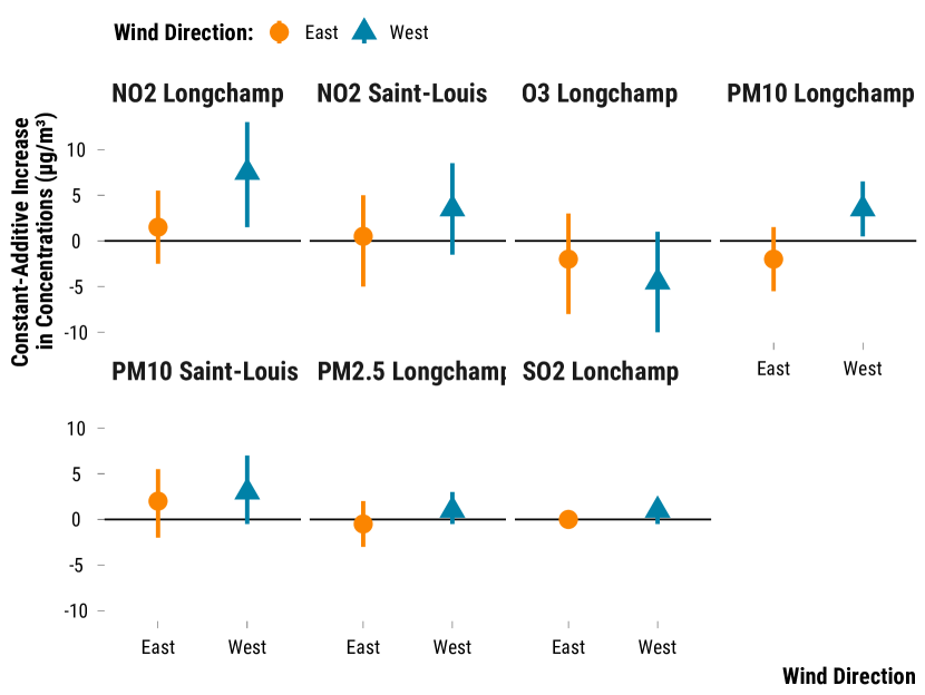
Figure A.3: Effects of Cruise Vessel Traffic on Pollutant Concentrations at the Hourly Level by Wind Directions.

Notes: Dots represent the point estimate for the immediate effect of cruise traffic on hourly pollutant concentration. Lines are 95% Fisherian intervals of constant treatment effects consistent with the data. Orange lines represent the effects for winds blowing from the East while orange lines represent effects for winds blowing from the West.

References

- (1)
- Abadie et al. (2020) Abadie, Alberto, Susan Athey, Guido W Imbens, and Jeffrey M Wooldridge (2020) “Sampling-Based versus Design-Based Uncertainty in Regression Analysis,” Econometrica, 88 (1), 265–296.
- Athey and Imbens (2017) Athey, Susan and Guido W Imbens (2017) “The econometrics of randomized experiments,” in Handbook of economic field experiments, 1, 73–140: Elsevier.
- AtmoSud (2018) AtmoSud (2018) “Quelle qualité de l’air pour les riverains des ports de Nice et Marseille?”Technical report, Technical Report.
- Atmosud (2019) Atmosud (2019) “Quelle qualité de l’air pour les riverains des ports de Nice et Marseille? Campagnes de mesure 2018,”Technical report, Atmosud, https://www.atmosud.org/sites/paca/files/atoms/files/200511_synthese_travaux_ports_2018_0.pdf.
- Baccini et al. (2017) Baccini, Michela, Alessandra Mattei, Fabrizia Mealli, Pier Alberto Bertazzi, and Michele Carugno (2017) “Assessing the short term impact of air pollution on mortality: a matching approach,” Environmental Health, 16 (1), 1–12.
- Bauernschuster et al. (2017) Bauernschuster, Stefan, Timo Hener, and Helmut Rainer (2017) “When labor disputes bring cities to a standstill: The impact of public transit strikes on traffic, accidents, air pollution, and health,” American Economic Journal: Economic Policy, 9 (1), 1–37.
- Bind (2019) Bind, Marie-Abèle (2019) “Causal modeling in environmental health,” Annual review of public health, 40, 23–43.
- Bind and Rubin (2019) Bind, Marie-Abèle C. and Donald B. Rubin (2019) “Bridging observational studies and randomized experiments by embedding the former in the latter,” Statistical Methods in Medical Research, 28 (7), 1958–1978.
- Bove et al. (2014) Bove, MC, P Brotto, F Cassola, E Cuccia, D Massabò, A Mazzino, A Piazzalunga, and P Prati (2014) “An integrated PM2.5 source apportionment study: Positive Matrix Factorisation vs. the chemical transport model CAMx,” Atmospheric Environment, 94, 274–286.
- Bowers and Leavitt (2020) Bowers, Jake and Thomas Leavitt (2020) “Causality and Design-Based Inference,” in The SAGE Handbook of Research Methods in Political Science and International Relations, 769–804: SAGE Publications Ltd.
- Bowers and Panagopoulos (2011) Bowers, Jake and Costas Panagopoulos (2011) “Fisher’s randomizationmode of statistical inference, then and now.,” Working Paper.
- Branson (2021) Branson, Zach (2021) “Randomization Tests to Assess Covariate Balance When Designing and Analyzing Matched Datasets,” Observational Studies, 7 (2), 1–36.
- CAIMAN (2015) CAIMAN (2015) “Air quality impact and greenhouse gases assessment for cruise and passenger ships,”Technical report, Technical Report.
- Cattaneo et al. (2015) Cattaneo, Matias D, Brigham R Frandsen, and Rocio Titiunik (2015) “Randomization inference in the regression discontinuity design: An application to party advantages in the US Senate,” Journal of Causal Inference, 3 (1), 1–24.
- Caughey et al. (2021) Caughey, Devin, Allan Dafoe, Xinran Li, and Luke Miratrix (2021) “Randomization Inference beyond the Sharp Null: Bounded Null Hypotheses and Quantiles of Individual Treatment Effects,” arXiv preprint arXiv:2101.09195.
- Chrisafis (2018) Chrisafis, Angelique (2018) “’I don’t want ships to kill me’: Marseille fights cruise liner pollution,” The Guardian, https://www.theguardian.com/environment/2017/jul/31/heading-to-venice-dont-forget-your-pollution-mask.
- Cleveland (1993) Cleveland, William S (1993) Visualizing data: Hobart press.
- Cochran and Rubin (1973) Cochran, William G. and Donald B. Rubin (1973) “Controlling bias in observational studies: A review,” Sankhyā: The Indian Journal of Statistics, Series A, 417–446.
- Cohen and Dupas (2010) Cohen, Jessica and Pascaline Dupas (2010) “Free distribution or cost-sharing? Evidence from a randomized malaria prevention experiment,” The Quarterly Journal of Economics, 1–45.
- Contini et al. (2011) Contini, D, A Gambaro, F Belosi, S De Pieri, WRL Cairns, A Donateo, E Zanotto, and M Citron (2011) “The direct influence of ship traffic on atmospheric PM2. 5, PM10 and PAH in Venice,” Journal of Environmental Management, 92 (9), 2119–2129.
- Corbett et al. (2007) Corbett, James J., James J. Winebrake, Erin H. Green, Prasad Kasibhatla, Veronika Eyring, and Axel Lauer (2007) “Mortality from ship emissions: a global assessment,” Environmental science & technology, 41 (24), 8512–8518.
- Dasgupta and Rubin (2021) Dasgupta, Tirthankar and Donald B. Rubin (2021) Experimental Design: A Randomization-Based Perspective: Unpublished Textbook.
- Dasgupta and Rubin (Fall 2015) Dasgupta, Tirthankar and Donald B Rubin (Fall 2015) STAT 240: Matched Sampling and Study Design: Harvard university.
- Diesch et al. (2013) Diesch, J-M, F Drewnick, T Klimach, and S Borrmann (2013) “Investigation of gaseous and particulate emissions from various marine vessel types measured on the banks of the Elbe in Northern Germany,” Atmospheric Chemistry and Physics, 13 (7), 3603–3618.
- Ding et al. (2016) Ding, Peng, Avi Feller, and Luke Miratrix (2016) “Randomization inference for treatment effect variation,” Journal of the Royal Statistical Society: Series B (Statistical Methodology), 78 (3), 655–671.
- Eckhardt et al. (2013) Eckhardt, Sabine, Ove Hermansen, Henrik Grythe, Markus Fiebig, Kerstin Stebel, Massimo Cassiani, Are Bäcklund, and Andreas Stohl (2013) “The influence of cruise ship emissions on air pollution in Svalbard–a harbinger of a more polluted Arctic?” Atmospheric Chemistry and Physics, 13 (16), 8401–8409.
- Fisher et al. (1937) Fisher, Ronald Aylmer et al. (1937) “The design of experiments.,” The design of experiments.
- Fogarty (2020) Fogarty, Colin B (2020) “Studentized sensitivity analysis for the sample average treatment effect in paired observational studies,” Journal of the American Statistical Association, 115 (531), 1518–1530.
- Forastiere et al. (2020) Forastiere, Laura, Michele Carugno, and Michela Baccini (2020) “Assessing short-term impact of PM 10 on mortality using a semiparametric generalized propensity score approach,” Environmental Health, 19 (1), 1–13.
- Friedrich (2017) Friedrich, Axel (2017) “Heading to Venice? Don’t forget your pollution mask,” The Guardian, https://www.theguardian.com/environment/2017/jul/31/heading-to-venice-dont-forget-your-pollution-mask.
- Gelman and Carlin (2014) Gelman, Andrew and John Carlin (2014) “Beyond power calculations: Assessing type S (sign) and type M (magnitude) errors,” Perspectives on Psychological Science, 9 (6), 641–651.
- Gelman et al. (2020) Gelman, Andrew, Jennifer Hill, and Aki Vehtari (2020) Regression and other stories: Cambridge University Press.
- Gerber and Green (2012) Gerber, Alan S and Donald P Green (2012) Field experiments: Design, analysis, and interpretation: WW Norton.
- Giaccherini et al. (2021) Giaccherini, Matilde, Joanna Kopinska, and Alessandro Palma (2021) “When particulate matter strikes cities: Social disparities and health costs of air pollution,” Journal of Health Economics, 78, 102478.
- Godzinski et al. (2019) Godzinski, Alexandre, M Suarez Castillo et al. (2019) “Short-term health effects of public transport disruptions: air pollution and viral spread channels,”Technical report, Institut National de la Statistique et des Etudes Economiques.
- Greifer and Stuart (2021) Greifer, Noah and Elizabeth A Stuart (2021) “Matching methods for confounder adjustment: an addition to the epidemiologist’s toolbox,” Epidemiologic reviews, 43 (1), 118–129.
- Gutman et al. (2012) Gutman, R, DB Rubin, and Stijn Vansteelandt (2012) “Analyses that Inform Policy Decisions [with Discussions],” Biometrics, 68 (3), 671–678.
- Hansen-Lewis and Marcus (2022) Hansen-Lewis, Jamie and Michelle M Marcus (2022) “Uncharted Waters: Effects of Maritime Emission Regulation,”Technical report, National Bureau of Economic Research.
- Heß (2017) Heß, Simon (2017) “Randomization inference with Stata: A guide and software,” The Stata Journal, 17 (3), 630–651.
- Ho and Imai (2006) Ho, Daniel E and Kosuke Imai (2006) “Randomization inference with natural experiments: An analysis of ballot effects in the 2003 California recall election,” Journal of the American statistical association, 101 (475), 888–900.
- Ho et al. (2007) Ho, Daniel E, Kosuke Imai, Gary King, and Elizabeth A Stuart (2007) “Matching as nonparametric preprocessing for reducing model dependence in parametric causal inference,” Political analysis, 15 (3), 199–236.
- Holland (1986) Holland, Paul W (1986) “Statistics and causal inference,” Journal of the American statistical Association, 81 (396), 945–960.
- Imbens (2015) Imbens, Guido W (2015) “Matching methods in practice: Three examples,” Journal of Human Resources, 50 (2), 373–419.
- Imbens and Rubin (2015) Imbens, Guido W and Donald B Rubin (2015) Causal inference in statistics, social, and biomedical sciences: Cambridge University Press.
- Keele et al. (2012) Keele, Luke, Corrine McConnaughy, and Ismail White (2012) “Strengthening the experimenter’s toolbox: Statistical estimation of internal validity,” American Journal of Political Science, 56 (2), 484–499.
- Keele and Miratrix (2019) Keele, Luke and Luke Miratrix (2019) “Randomization inference for outcomes with clumping at zero,” The American Statistician, 73 (2), 141–150.
- King and Zeng (2006) King, Gary and Langche Zeng (2006) “The dangers of extreme counterfactuals,” Political analysis, 14 (2), 131–159.
- Klotz and Berazneva (2022) Klotz, Richard and Julia Berazneva (2022) “Local Standards, Behavioral Adjustments, and Welfare: Evaluating California’s Ocean-Going Vessel Fuel Rule,” Journal of the Association of Environmental and Resource Economists, 9 (3), 383–424.
- Knittel et al. (2016) Knittel, Christopher R, Douglas L Miller, and Nicholas J Sanders (2016) “Caution, drivers! Children present: Traffic, pollution, and infant health,” Review of Economics and Statistics, 98 (2), 350–366.
- Lee et al. (2021) Lee, Kwonsang, Dylan S Small, and Francesca Dominici (2021) “Discovering heterogeneous exposure effects using randomization inference in air pollution studies,” Journal of the American Statistical Association, 116 (534), 569–580.
- Liu et al. (2016) Liu, Huan, Mingliang Fu, Xinxin Jin, Yi Shang, Drew Shindell, Greg Faluvegi, Cary Shindell, and Kebin He (2016) “Health and climate impacts of ocean-going vessels in East Asia,” Nature Climate Change, 6 (11), 10.1038/nclimate3083.
- Liu et al. (2019) Liu, Huan, Zhi-Hang Meng, Zhao-Feng Lv et al. (2019) “Emissions and health impacts from global shipping embodied in US–China bilateral trade,” Nature Sustainability, 2 (11), 10.1038/s41893-019-0414-z.
- Lu et al. (2019) Lu, Jiannan, Yixuan Qiu, and Alex Deng (2019) “A note on Type S/M errors in hypothesis testing,” British Journal of Mathematical and Statistical Psychology, 72 (1), 1–17.
- MacKinnon and Webb (2020) MacKinnon, James G and Matthew D Webb (2020) “Randomization inference for difference-in-differences with few treated clusters,” Journal of Econometrics, 218 (2), 435–450.
- Mayer (2019) Mayer, Michael (2019) missRanger: Fast Imputation of Missing Values, https://cran.r-project.org/package=missRanger, R package version 2.1.0.
- Merico et al. (2016) Merico, E, A Donateo, A Gambaro et al. (2016) “Influence of in-port ships emissions to gaseous atmospheric pollutants and to particulate matter of different sizes in a Mediterranean harbour in Italy,” Atmospheric Environment, 139, 1–10.
- Merico et al. (2017) Merico, Eva, Andrea Gambaro, A Argiriou et al. (2017) “Atmospheric impact of ship traffic in four Adriatic-Ionian port-cities: Comparison and harmonization of different approaches,” Transportation Research Part D: Transport and Environment, 50, 431–445.
- Micali and Vazirani (1980) Micali, Silvio and Vijay V Vazirani (1980) “An O (v v c E) algorithm for finding maximum matching in general graphs,” in 21st Annual Symposium on Foundations of Computer Science (sfcs 1980), 17–27, IEEE.
- Mocerino et al. (2020) Mocerino, Luigia, Fabio Murena, Franco Quaranta, and Domenico Toscano (2020) “A methodology for the design of an effective air quality monitoring network in port areas,” Scientific Reports, 10 (1), 1–10.
- Moretti and Neidell (2011) Moretti, Enrico and Matthew Neidell (2011) “Pollution, health, and avoidance behavior evidence from the ports of Los Angeles,” Journal of Human Resources, 46 (1), 154–175.
- Mueller et al. (2011) Mueller, Daniel, Stefanie Uibel, Masaya Takemura, Doris Klingelhoefer, and David A Groneberg (2011) “Ships, ports and particulate air pollution-an analysis of recent studies,” Journal of Occupational Medicine and Toxicology, 6 (1), 1–6.
- Murena et al. (2018) Murena, F, L Mocerino, F Quaranta, and D Toscano (2018) “Impact on air quality of cruise ship emissions in Naples, Italy,” Atmospheric Environment, 187, 70–83.
- Neyman (1923) Neyman, Jerzy (1923) “Sur les applications de la thar des probabilities aux experiences Agaricales: Essay des principle. Excerpts reprinted (1990) in English,” Statistical Science, 5 (463-472), 4.
- Piga et al. (2013) Piga, Damien, Alexandre Armengaud, Magali Devèze, Michael Parra, Nicolas Marchand, Anaïs Detournay, and Salameh Dalia (2013) “Synthèse du projet APICE - Marseille,”Technical report, Technical Report.
- Rosenbaum (2018) Rosenbaum, Paul (2018) Observation and experiment: Harvard University Press.
- Rosenbaum et al. (2010) Rosenbaum, Paul R et al. (2010) Design of observational studies, 10: Springer.
- Rosenbaum (1987) Rosenbaum, Paul R (1987) “Sensitivity analysis for certain permutation inferences in matched observational studies,” Biometrika, 74 (1), 13–26.
- Rubin (1974) Rubin, Donald B (1974) “Estimating causal effects of treatments in randomized and nonrandomized studies.,” Journal of Educational Psychology, 66 (5), 688.
- Rubin (1978) (1978) “Bayesian inference for causal effects: The role of randomization,” The Annals of Statistics, 34–58.
- Rubin (1991) (1991) “Practical implications of modes of statistical inference for causal effects and the critical role of the assignment mechanism,” Biometrics, 1213–1234.
- Rubin (2005) (2005) “Causal inference using potential outcomes: Design, modeling, decisions,” Journal of the American Statistical Association, 100 (469), 322–331.
- Rubin (2006) (2006) Matched sampling for causal effects: Cambridge University Press.
- Rubin (2008) (2008) “For objective causal inference, design trumps analysis,” The annals of applied statistics, 2 (3), 808–840.
- Schlenker and Walker (2016) Schlenker, Wolfram and W Reed Walker (2016) “Airports, air pollution, and contemporaneous health,” The Review of Economic Studies, 83 (2), 768–809.
- Sekhon (2009) Sekhon, Jasjeet S (2009) “Opiates for the matches: Matching methods for causal inference,” Annual Review of Political Science, 12, 487–508.
- Simeonova et al. (2021) Simeonova, Emilia, Janet Currie, Peter Nilsson, and Reed Walker (2021) “Congestion pricing, air pollution, and children’s health,” Journal of Human Resources, 56 (4), 971–996.
- Sommer et al. (2018) Sommer, Alice J, Mihye Lee, and Marie-Abèle C Bind (2018) “Comparing apples to apples: an environmental criminology analysis of the effects of heat and rain on violent crimes in Boston,” Palgrave communications, 4 (1), 1–10.
- Sommer et al. (2021) Sommer, Alice J, Emmanuelle Leray, Young Lee, and Marie-Abèle C Bind (2021) “Assessing environmental epidemiology questions in practice with a causal inference pipeline: An investigation of the air pollution-multiple sclerosis relapses relationship,” Statistics in Medicine, 40 (6), 1321–1335.
- Sorte et al. (2020) Sorte, Sandra, Vera Rodrigues, Carlos Borrego, and Alexandra Monteiro (2020) “Impact of harbour activities on local air quality: A review,” Environmental Pollution, 257, 113542.
- Splawa-Neyman et al. (1990) Splawa-Neyman, Jerzy, Dorota M Dabrowska, and TP Speed (1990) “On the application of probability theory to agricultural experiments. Essay on principles. Section 9.,” Statistical Science, 465–472.
- Stuart (2010) Stuart, Elizabeth A (2010) “Matching methods for causal inference: A review and a look forward,” Statistical science: a review journal of the Institute of Mathematical Statistics, 25 (1), 1.
- Timm (2019) Timm, Andrew (2019) retrodesign: Tools for Type S (Sign) and Type M (Magnitude) Errors, https://CRAN.R-project.org/package=retrodesign, R package version 0.1.0.
- Tufte (1985) Tufte, Edward R (1985) “The visual display of quantitative information,” The Journal for Healthcare Quality (JHQ), 7 (3), 15.
- Tukey et al. (1977) Tukey, John W et al. (1977) Exploratory data analysis, 2: Reading, MA.
- Viana et al. (2014) Viana, Mar, Pieter Hammingh, Augustin Colette, Xavier Querol, Bart Degraeuwe, Ina de Vlieger, and John van Aardenne (2014) “Impact of maritime transport emissions on coastal air quality in Europe,” Atmospheric Environment, 90, 96–105.
- Viana et al. (2008) Viana, Mar, Thomas AJ Kuhlbusch, Xavier Querol et al. (2008) “Source apportionment of particulate matter in Europe: a review of methods and results,” Journal of Aerosol Science, 39 (10), 827–849.
- Wu and Ding (2021) Wu, Jason and Peng Ding (2021) “Randomization tests for weak null hypotheses in randomized experiments,” Journal of the American Statistical Association, 116 (536), 1898–1913.
- Zhao and Ding (2021) Zhao, Anqi and Peng Ding (2021) “Covariate-adjusted Fisher randomization tests for the average treatment effect,” Journal of Econometrics, 225 (2), 278–294.
- Zhong et al. (2017) Zhong, Nan, Jing Cao, and Yuzhu Wang (2017) “Traffic congestion, ambient air pollution, and health: Evidence from driving restrictions in Beijing,” Journal of the Association of Environmental and Resource Economists, 4 (3), 821–856.
- Zhu and Wang (2021) Zhu, Junming and Jiali Wang (2021) “The effects of fuel content regulation at ports on regional pollution and shipping industry,” Journal of Environmental Economics and Management, 106, 102424.
- Zigler and Dominici (2014) Zigler, Corwin Matthew and Francesca Dominici (2014) “Point: clarifying policy evidence with potential-outcomes thinking—beyond exposure-response estimation in air pollution epidemiology,” American journal of epidemiology, 180 (12), 1133–1140.