A Yosida’s parametrix approach to Varadhan’s estimates for a degenerate diffusion under the weak Hörmander condition

Abstract

We adapt and extend Yosida’s parametrix method, originally introduced for the construction of the fundamental solution to a parabolic operator on a Riemannian manifold, to derive Varadhan-type asymptotic estimates for the transition density of a degenerate diffusion under the weak Hörmander condition. This diffusion process, widely studied by Yor in a series of papers, finds direct application in the study of a class of path-dependent financial derivatives known as Asian options. We obtain the Varadhan formula

$$\frac{-2\log p(t,x;T,y)}{\Psi(t,x;T,y)}\to 1,\qquad\text{as }\quad T-t\to 0^{+},$$ (0.1)

where $p$ denotes the transition density and $\Psi$ denotes the optimal cost function of a deterministic control problem associated to the diffusion. We provide a partial proof of this formula, and present numerical evidence to support the validity of an intermediate inequality that is required to complete the proof. We also derive an asymptotic expansion of the cost function $\Psi$, expressed in terms of elementary functions, which is useful in order to design efficient approximation formulas for the transition density.

Keywords: weak Hörmander condition, asymptotic estimates, parametrix, hypoelliptic diffusion, Asian options.

1 Introduction

We consider the system of Itô stochastic differential equations (SDEs)

$$\begin{cases}dX^{1}_{s}={\sigma}X^{1}_{s}dW_{s},\qquad&X^{1}_{t}=x_{1}\\ dX^{2}_{s}=X^{1}_{s}ds,\qquad&X^{2}_{t}=x_{2}\end{cases},$$ (1.1)

where ${\sigma}$ is a positive constant. The study of this equation is motivated by the financial problem of pricing arithmetically averaged Asian options. Indeed, the process $\left(X_{s}^{1}\right)_{s\geq t}$ is a geometric Brownian motion starting from $x_{1}$ at $s=t$, and describes the evolution of the price of some financial asset in the Black-Scholes setting, while $\left(X_{s}^{2}\right)_{s\geq t}$ is the time-integral of $\left(X_{s}^{1}\right)_{s\geq t}$ and appears whenever the payoff of the option depends on the past average of the asset price. We refer to Section 1.3 below for a more detailed discussion of the related applications.

Although the explicit expression of the solution to (1.1) is well known, namely

$$\begin{cases}X^{1}_{s}=x_{1}e^{\sigma(W_{s}-W_{t})-\frac{{\sigma}^{2}}{2}(s-t)}\\ X^{2}_{s}=x_{2}+\int_{t}^{s}X^{1}_{\tau}d\tau\end{cases},\qquad s>t,$$ (1.2)

the analytical study of its density is more involved. We recall that Yor provided us with the following closed-form expression for the joint density of the process $X=(X^{1},X^{2})$ with $\sigma=1$ starting from $(1,0)$ at time $0$:

$$p(s,y_{1},y_{2})=\frac{e^{\frac{\pi^{2}}{2s}}}{\pi y_{2}^{2}\sqrt{2\pi s}}\exp\left(-\frac{1+y_{1}^{2}}{2y_{2}}\right)q\left(s,\frac{{y_{1}}}{y_{2}}\right),$$ (1.3)

for $s,y_{1},y_{2}>0$, where

$$q\left(s,\eta\right)=\int_{0}^{\infty}e^{-\frac{\xi^{2}}{2s}}e^{-\eta\cosh(\xi)}\sinh{(\xi)}\sin\left(\frac{\pi\xi}{s}\right)d\xi.$$ (1.4)

This expression was first obtained in [36]. We also refer to [24, Theorem 4.1] for a more compact statement and a concise proof. Note that the density $p$ is trivially null for non-positive values of $y_{1}$ and $y_{2}$, as the process $X^{1}$ is strictly positive. Furthermore, an elementary change of variable (see (2.8)-(2.9) below) allows to write the transition density $p(t,x_{1},x_{2};s,y_{1},y_{2})$ of the process $X=(X^{1},X^{2})$ for a general $\sigma>0$ starting from $(x_{1},x_{2})$ at time $t$, which is constantly null if $y_{1}\leq 0$ or $y_{2}\leq x_{2}$.

Although (1.3) provides a semi-closed-form expression for the density, the latter is notoriously hard to handle from the numerical and analytical point of view. On the one hand, the numerical integration of the density as written in (1.3) is not accurate when the time $s$ is close to $0$, and this results in relevant errors when computing the price of financial options; we refer to Section 1.3 for more details and appropriate references about this problem. On the other hand, it is difficult to extract relevant analytical information, such as asymptotic properties of the density for extreme values of $(y_{1},y_{2})$ and small values of time $s$. We undertake the study of these issues by following a different approach, namely we study the transition density as the fundamental solution of the associated backward Kolmogorov ultra-parabolic operator

$$\mathscr{L}={\partial_{t}+x_{1}\partial_{x_{2}}}+\frac{{\sigma}^{2}x_{1}^{2}}{2}\partial_{x_{1}x_{1}},\qquad(t,x_{1},x_{2})\in{\mathbb{R}}\times D,$$ (1.5)

where we set $D:={\mathbb{R}}^{+}\times{\mathbb{R}}$, with ${\mathbb{R}}^{+}:=]0,+\infty[$. The operator $\mathscr{L}$ is hypoelliptic in that it can be written in Hörmander form as $\mathscr{L}=Y-\frac{\sigma}{2}Z+\frac{1}{2}Z^{2}$ with the vector fields

$$Y=\partial_{t}+x_{1}\partial_{x_{2}},\qquad Z={\sigma}x_{1}\partial_{x_{1}}$$ (1.6)

satisfying the Hörmander condition (see Section 1.1). Note that the commutator $[Z,Y]$ is necessary in order to span the space ${\mathbb{R}}^{3}$. In the Probability community this is often referred to as weak Hörmander condition.

In [5] the authors showed that the transition density of $(X^{1},X^{2})$ coincides with the fundamental solution $p=p(t,x;T,y)$ for $\mathscr{L}$, and derived upper and lower bounds in terms of the optimal cost function $\Psi$, defined as the solution of the control problem given by:

$$\Psi(t,x;T,y)=\min_{\omega}\int_{t}^{T}|\omega(s)|^{2}ds,$$ (1.7)

where the minimum is taken over all controls $\omega\in L^{2}([t,T])$ such that the problem

$$\begin{cases}\dot{\gamma}_{1}(s)=\sigma\omega(s)\gamma_{1}(s)\\ \dot{\gamma}_{2}(s)=\gamma_{1}(s)\end{cases}t<s<T,\qquad\text{and}\quad\begin{cases}\gamma_{1}(t)=x_{1},\ \gamma_{1}(T)=y_{1}\\ \gamma_{2}(t)={x_{2}},\ \gamma_{2}(T)=y_{2}\end{cases}$$ (1.8)

admits a solution. Such a control exists if and only if $x_{2}<y_{2}$. As usual in control theory, we agree to set $\Psi(z;w):=+\infty$ whenever $x_{2}>y_{2}$, in accordance with the fact that $p(t,x;T,y)$ is null.

Roughly speaking, the main results in [5] are an explicit representation for the cost function $\Psi$ and the following upper-lower bounds:

$$\frac{c}{{\sigma}^{2}y_{1}^{2}(T-t)^{2}}e^{-\frac{C}{2}\Psi(z;w)}\leq p(z;w)\leq\frac{C}{{\sigma}^{2}y_{1}^{2}(T-t)^{2}}e^{-\frac{c}{2}\Psi(z;w)}$$ (1.9)

for some positive constants $C>>1$ and $c<<1$, and for $z=(t,x),w=(T,y)$ such that $t<T$ and $x_{2}<y_{2}$. We improve such bounds by proving that the constants appearing at the exponent in both sides of (1.9) are equal to one, namely

$$\log p(z;w)\sim-\frac{\Psi(z;w)}{2},\qquad\text{as }\quad T-t\to 0^{+},$$ (1.10)

where we agree to let

$$f\sim g\qquad\text{if}\quad\frac{f}{g}\to 1.$$ (1.11)

For clarity we state two separate results for the upper and lower upper bounds, respectively. We anticipate that one step of the proof of such estimates relies on some bounds, precisely the Key Inequalities 4.5 below, which we prove numerically in Section 5. We refer to Section 1.2 for a preliminary discussion about the interpretation of such inequalities.

Theorem 1.1 (Upper bound).

If the Key Inequalities 4.5 hold, then for any $\tau>0$ there exists a positive constant $C>0$, only dependent on $\tau$ and $\sigma$, such that

$$p(z;w)\leq C\,\frac{\sqrt{{\bf h}(z;w)}+{\bf h}(z;w)}{{\sigma}^{2}y_{1}^{2}(T-t)^{2}}e^{-\frac{1}{2}\Psi(z;w)},$$ (1.12)

for any $z=(t,x_{1},x_{2}),w=(T,y_{1},y_{2})\in{\mathbb{R}}\times D$ such that $T-\tau<t<T$ and $x_{2}<y_{2}$, where

$${\bf h}(z;w):=\frac{(T-t)\sqrt{x_{1}y_{1}}}{y_{2}-x_{2}},$$ (1.13)

and $\Psi$ is the cost function defined as the solution of the control problem above, whose explicit representation is given in (2.15).

Theorem 1.2 (Lower bound).

If the Key Inequalities 4.5 hold, then for any ${\varepsilon},\kappa>0$ there exists $\tau>0$, only dependent on ${\varepsilon}$, $\kappa$ and $\sigma$, such that

$$p(z;w)\geq(1-{\varepsilon})\,\frac{{\bf h}(z;w)}{{\sigma}^{2}y_{1}^{2}(T-t)^{2}}e^{-\frac{1}{2}\Psi(z;w)},$$ (1.14)

for any $z=(t,x_{1},x_{2}),w=(T,y_{1},y_{2})\in{\mathbb{R}}\times D$ such that $T-\tau<t<T$, $x_{2}<y_{2}$ and $\frac{1}{\kappa}\leq\frac{\sqrt{x_{1}y_{1}}}{y_{2}-x_{2}}<\kappa$.

The results above are obtained by adapting to the strictly hypoelliptic setting the Yosida’s parametrix method ([37]) for the construction of the fundamental solution to parabolic-type operators. Specifically, we use the cost function $\Psi$ to define a parametrix function. We believe that this method might be of separate interest and we refer to Section 1.2 for further details and related references.

The interest in the results above is duplex. From the theoretical point of view, they provide Varadhan-type estimates for a degenerate operator satisfying a weak Hörmander condition. A detailed discussion about this aspect is deferred to Section 1.1 below. Secondly, knowing the sharp choice of the constant in the exponent paves the way for developing numerically tractable asymptotic expansions of the transition density: we discuss this possible application in Section 1.3.

With regard to the latter point, the computational aspects of the cost function $\Psi$ are also important. In [5] the Authors solved the control problem (1.7)-(1.8) and provided an explicit representation of $\Psi$, which we report in Section 2. Tough exact, such expression involves the inverse of hyperbolic trigonometric functions. In Section 3 we derive an expansion for the the cost function $\Psi$ whose terms only contain elementary functions, namely

$$\Psi(z;\zeta)=\frac{4}{{\sigma}^{2}(T-t)}\bigg{[} {\bf h}(z,w)\bigg{(}\sqrt{\frac{y_{1}}{x_{1}}}+\sqrt{\frac{x_{1}}{y_{1}}}-2\bigg{)}$$ (1.15)

$$+\sum_{n=2}^{\infty}a_{n}{\bf 1}_{[1,\infty[}\big{(}{\bf h}(z,w)\big{)}\frac{\big{(}{\bf h}(z,w)-1\big{)}^{n}}{\big{(}{\bf h}(z,w)\big{)}^{n-1}}+b_{n}{\bf 1}_{]0,1[}\big{(}{\bf h}(z,w)\big{)}\frac{\big{(}-\log{\bf h}(z,w)\big{)}^{n}}{\big{(}1-\log{\bf h}(z,w)\big{)}^{n-2}}\bigg{]},$$ (1.16)

with ${\bf h}(z,w)$ as defined in (1.13), and where the coefficients $a_{n},b_{n}$ can be computed recursively (see Proposition 3.3). A remarkable feature of such expansion is that it seems both point-wise and asymptotically convergent, in the sense that it approximates the asymptotic behavior of $\Psi(z;\zeta)$ as ${\bf h}(z,w)$ approaches $0$ and $+\infty$. In Section 3 we managed to prove point-wise convergence for ${\bf h}(z;\zeta)>0$ and asymptotic convergence as ${\bf h}(z,w)\to+\infty$.

After Sections 1.1, 1.2 and 1.3 below, the remainder of the paper unfolds as follows. Section 2 contains some preliminaries about the cost function $\Psi$ and the fundamental solution of $\mathscr{L}$. In Section 3 we derive the representation (LABEL:eq:rep_Psi_intro) and provide a partial proof of convergence. In Section 4 we prove Theorems 1.1 and 1.2 by extending Yosida’s parametrix method. Section 5 contains the numerical evidence supporting the validity of the Key Inequalities 4.5. Appendices A and B contain, respectively, a topological lemma needed to prove the results of Section 3 and the proof of Lemma 4.1 appearing in Section 4.

1.1 Varadhan-type estimates

In order to firm our results within the existing literature about fundamental solution, and density, estimates, let us consider the non-divergence-form second-order differential operator

$$\mathscr{H}=\frac{1}{2}\sum_{i,j=1}^{n}a_{ij}(t,x)\partial_{x_{i}x_{j}}+\sum_{i=1}^{n}\mu_{i}(t,x)\partial_{x_{i}}+\partial_{t},\qquad(t,x)\in{\mathbb{R}}\times\widetilde{D},$$ (1.18)

with $\widetilde{D}$ being a domain of ${\mathbb{R}}^{n}$. Clearly, the operator $\mathscr{L}$ in (1.5) is a particular instance of (1.18). From the probabilistic stand-point, under suitable assumptions, $\mathscr{H}$ is the extended generator of a solution to the following Itô SDE:

$$dX_{s}=\mu(t,X_{s})ds+{\sigma}(t,X_{s})dW_{s},\qquad X_{t}=x,$$ (1.19)

with $W$ being a $n$-dimensional Brownian motion, and $\sigma$ a $n\times n$ matrix such that $\sigma\sigma^{\top}=a=(a_{i,j})_{i,j=1,\cdots,n}$. Also, the transition density of $X$, hereafter denoted by $p=p(t,x;T,y)$, coincides with the fundamental solution of $\mathscr{H}$.

In the uniformly parabolic case, a fairly general classical result (see [13]) states that

$$\frac{c}{(T-t)^{n/2}}e^{-\frac{C|y-x|^{2}}{2(T-t)}}\leq p(t,x;T,y)\leq\frac{C}{(T-t)^{n/2}}e^{-\frac{c|y-x|^{2}}{2(T-t)}},\qquad t<T,\quad x,y\in{\mathbb{R}}^{n},$$ (1.20)

where $c,C$ are positive constants independent of $(t,x),(T,y)$. These estimates can be proved under boundedness and Hölder regularity assumptions on the coefficients of $\mathscr{H}$, and assuming a uniform ellipticity condition on the second-order coefficients $a_{ij}$. More precisely, the upper-bound above can be obtained by means of the so-called parametrix method. With the same method it is possible to prove the lower bound in (1.20), but only locally in space: the global version can be achieved with the method of the Harnack chains, introduced by Aronson in [1], which is based on the Harnack inequality. Though very general, the bounds in (1.20) are not sharp enough to characterize the asymptotic behavior for small times of the fundamental solution $p$ away from the pole. In the groundbreaking paper [34] Varadhan proved, for $\mu\equiv 0$ and $a(t,x)=a(x)$, that

$$\lim_{T-t\to 0^{+}}2(T-t)\,{\log p(t,x;T,y)}=-d^{2}(x,y),$$ (1.21)

uniformly with respect to $x,y$ over a compact subset of ${\mathbb{R}}^{n}$, where $d$ represents the geodesic distance with respect to the Riemann metric $a^{-1}(x)dx_{i}dx_{j}$, namely

$$d(x,y)=\inf_{\gamma:\gamma(0)=x,\,\gamma(1)=y}\int_{0}^{1}\sqrt{\big{\langle}a^{-1}\big{(}\gamma(s)\big{)}\dot{\gamma}(s),\dot{\gamma}(s)\big{\rangle}}\,ds.$$ (1.22)

The assumptions in [34] are, again, uniform ellipticity and Hölder continuity for the second-order coefficients. Note that (1.21) is more precise than (1.20), in that it yields the exact asymptotic behavior of the logarithm of $p$ for small times. In the subsequent paper [33], building upon (1.21), Varadhan established a large-deviation principle for elliptic diffusions of the form (1.19). The cornerstone contributions [34]-[33] initiated a whole stream of literature, dealing with asymptotic expansions of the transition densities (or heat-kernels in the context of PDEs) of diffusion processes on Riemannian manifolds. Such expansions aim at characterizing the full asymptotic behavior of $p(t,x;T,y)$, under various assumptions on the underlying geometry, by adding up additional terms to the leading one given by (1.21). For instance, following the WKB (Wentzel-Kramers-Brillouin) method, one seeks representations of the type

$$p(t,x;T,y)=\frac{\exp\Big{(}\!-\frac{d^{2}(x,y)}{2(T-t)}\Big{)}}{(T-t)^{n/2}}\Big{(}\alpha_{0}(x,y)+(T-t)\alpha_{1}(x,y)+(T-t)^{2}\alpha_{2}(x,y)+\cdots\Big{)}.$$ (1.23)

We refer, for instance, to [25] and [2] for some relevant contributions to this field, which mainly developed in the years 1970s and 1980s. We also mention the important contribution of Freidlin and Wentzell (e.g. [35]) to the subject of large deviations for diffusion processes. In the last two decades, these asymptotic techniques were employed for the study of volatility models in mathematical finance (see [14] and the references therein).

In the late 1980s these results were generalized to the hypoelliptic setting, under the so-called strong Hörmander condition. To explain these generalizations, it is useful to write the operator $\mathscr{H}$ above (with time-independent coefficients) in Hörmander form, namely

$$\mathscr{H}=\partial_{t}+Z_{0}+\frac{1}{2}\sum_{j=1}^{m}Z_{j}^{2},$$ (1.24)

where $Z=(Z_{0},Z_{1},\dots,Z_{m})$ is a system of vector fields defined on a domain $\widetilde{D}\subset{\mathbb{R}}^{n}$ satisfying the strong Hörmander’s condition

$${\rm Lie}(Z_{1},\ldots,Z_{m})(x)={\mathbb{R}}^{n},\qquad x\in\widetilde{D},$$ (1.25)

where ${\rm Lie}(Z_{1},\ldots,Z_{m})$ is the Lie algebra generated by the vector fields $Z_{1},\ldots,Z_{m}$, namely the vector space spanned by $Z_{1},\ldots,Z_{m}$ and their commutators. Note that, if $\mathscr{H}$ represents the generator of $X$ in (1.19), then the vector field $Z_{j}$, $j=1,\cdots,m$, is exactly identified by the $j$-th column of the diffusion matrix $\sigma$. Under the assumption of smooth vector fields, Leandre ([21], [22]) proved that (1.21) remains valid in this setting, with $d(x,t)$ being the Carnot-Caratheodory sub-Riemannian metric induced by the vector fields $Z_{1},\ldots,Z_{m}$. In [3] also (1.23) was extended to this setting. A contribution in this direction was also given in [6].

In order to discuss extensions to strictly hypoelliptic settings (when (1.25) fails), it is crucial the following

Remark 1.3.

Both in the Riemannian and sub-Riemannian case, (1.21) can also be written in the form of (1.10), where $\Psi$ represents here the solution of the optimal control problem given by (1.7), with the minimum taken over all controls $\omega\in L^{2}([t,T])$ such that the problem

$$\begin{cases}\dot{\gamma}(s)=\omega(s)\sigma\big{(}\gamma(s)\big{)},\quad t<s<T,\\ \gamma(t)=x,\ \gamma(T)=y\end{cases}$$ (1.26)

admits a solution. Indeed, it is a standard result (see for instance [33, Lemma 2.2] for the elliptic case) that

$$\frac{d^{2}(x,y)}{T-t}=\Psi(t,x;T,y).$$ (1.27)

Under the so-called weak Hörmander condition, namely

$${\rm Lie}(\partial_{t}+Z_{0},Z_{1},\ldots,Z_{m})(x)={\mathbb{R}}^{n+1},\qquad x\in\widetilde{D},$$ (1.28)

the hypoellipticity of the operator $\mathscr{H}$ is preserved, but the second-order vector fields $Z_{1},\ldots,Z_{m}$ and their commutators are no longer enough to span the space ${\mathbb{R}}^{n}$. Therefore, there is no sub-Riemannian metric on ${\mathbb{R}}^{n}$ and an estimate in the form of (1.21) can be no longer achieved. The cost function $\Psi$, however, remains well defined as the solution of the same control problem (1.7) where

$$\begin{cases}\dot{\gamma}(s)=\mu\big{(}\gamma(s)\big{)}+\omega(s)\sigma\big{(}\gamma(s)\big{)},\quad t<s<T,\\ \gamma(t)=x,\ \gamma(T)=y\end{cases}$$ (1.29)

replaces (1.26). Therefore, in light of Remark 1.3, (1.10) appears as the natural generalization of (1.21) to strictly hypoelliptic settings. In this sense, Theorems 1.1 and 1.2 above, which lead to (1.10), can be viewed as Varadhan-type estimates for the degenerate parabolic operator $\mathscr{L}$. As already mentioned above, (1.10) sharpens the estimates proved in [5] for the fundamental solution of $\mathscr{L}$. Furthermore, we are not aware of other Varadhan-type formulas in the context of hypoelliptic operators under the weak Hörmander condition.

Note that the drift coefficient $\mu$ in (1.29), which is not controlled, is needed to ensure the existence of a path connecting $x$ and $y$. Also, the fact that (1.27) does not hold in general is evident as $\Psi(t,x;T,y)$ can exhibit different rates of explosion, as $T-t\to 0^{+}$, depending on the choice of $(x,y)$. This is a well-known phenomenom, which reflects the different time-scales of the single components of the underlying diffusion. A stylized example is given by the stochastic Langevin equation

$$\begin{cases}dX^{1}_{s}=\sigma dW_{s},\qquad&X^{1}_{t}=x_{1}\\ dX^{2}_{s}=X^{1}_{s}ds,\qquad&X^{2}_{t}=x_{2}\end{cases}$$ (1.30)

with $\sigma$ positive constant, whose generator is given by

$$\mathscr{H}={\partial_{t}+x_{1}\partial_{x_{2}}}+\frac{a}{2}\partial_{x_{1}x_{1}},\qquad a=\sigma^{2}.$$ (1.31)

Its fundamental solution is given exactly by

$$p_{\sigma}(t,x;T,y) =\frac{1}{2\pi\sqrt{\text{det}\,{\bf C}(\sigma,T-t)}}\exp\bigg{(}{-\frac{1}{2}\Psi_{\sigma}(t,x;T,y)}\bigg{)},$$ (1.32)

$${\bf C}(\sigma,s) :=\sigma^{2}\begin{pmatrix}s&-\frac{s^{2}}{2}\\ -\frac{s^{2}}{2}&\frac{s^{3}}{3}\ \end{pmatrix},$$ (1.33)

where

$$\Psi_{\sigma}(t,x;T,y) =\big{\langle}{\bf C}^{-1}(\sigma,T-t)\big{(}x_{1}-y_{1},x_{2}-y_{2}+(T-t)y_{1}\big{)},\big{(}x_{1}-y_{1},x_{2}-y_{2}+(T-t)y_{1}\big{)}\big{\rangle}$$ (1.34)

$$=\frac{3\big{(}2(y_{2}-x_{2})-(T-t)(x_{1}+y_{1})\big{)}^{2}}{\sigma^{2}(T-t)^{3}}+\frac{(y_{1}-x_{1})^{2}}{\sigma^{2}(T-t)}$$ (1.35)

is the cost function of the associated control problem (see for instance [27, Example 9.53]).

1.2 Yosida’s parametrix

In order to obtain the bounds in Theorems 1.1 and 1.2, we adapt and extend the method introduced by Yosida in his seminal paper [37], where he outlined a geometrical variation of the classical Levi’s parametrix method for the construction of the fundamental solution of a parabolic-type operator $\mathscr{H}$ of type (1.18) on a Riemannian manifold. Such method, which was published 14 years before Varadhan’s paper [34], already contained the idea that an expansion like (1.23) should hold, and in particular that the logarithm of the fundamental solution $p$ should asymptotically behave like in (1.21). In spite of this, Yosida’s method did not become a standard tool in the study of the asymptotic properties of transition densities. We suspect this is partially due the fact that his construction was mainly heuristic: no precise assumptions on the coefficients were given to ensure convergence, nor upper/lower bounds leading to (1.21) were proved in [37]. In [16], Gatheral et al. brought Yosida’s method to the attention of the mathematical finance community emphasizing its versatility from the computational point of view, with a particular focus on its ability to deal with time-dependent coefficients. In this paper, inspired by [16], we push Yosida’s method one step further and adapt it to the strictly hypoelliptic setting. In Section 4 we perform the construction of the fundamental solution $p$ for the operator $\mathscr{L}$ in (1.5), and prove the estimates (1.12)-(1.14) which lead to (1.10). Although we treat here a special case, we claim that the principles of this approach can be employed in general for a wider class of degenerate parabolic operators under the weak Hörmander condition, to establish full expansions analogous to (1.23). The study of general assumptions on the coefficients, possibly time-dependent, under which this method yields rigorous results is subject of ongoing investigation.

Consider the parabolic operator $\mathscr{H}$ in (1.18), and assume for simplicity $\mu\equiv 0$ and $a_{ij}(t,x)=a(x)$. In the Yosida’s parametrix, the key difference with respect to Levi’s original method lies in the choice of the parametrix function (the starting point of the iterative construction), which is dependent on the geodesic distance $d$ induced by the second-order coefficients of the differential operator. Precisely, in Yosida’s method the kernel that defines the parametrix function is set as

$$\frac{(T-t)^{-n/2}}{\sqrt{(2\pi)^{n}\,\text{det}\,a(y)}}\exp\bigg{(}{-\frac{1}{2}\frac{d^{2}(x,y)}{T-t}}\bigg{)},$$ (1.36)

where $d$ is the Riemannian distance (1.22) induced by the coefficients $a_{ij}$. By opposite, in Levi’s method the parametrix function is the fundamental solution of the constant coefficients operator obtained from $\mathscr{H}$ by freezing the coefficients at $y$. In other words, the distance $d$ in (1.36) is replaced by the geodesic distance taken with respect to the constant metric tensor $a^{-1}(y)dx_{i}dx_{j}$, namely the kernel is

$$\frac{(T-t)^{-n/2}}{\sqrt{(2\pi)^{n}\,\text{det}\,a(y)}}\exp\bigg{(}{-\frac{1}{2}\frac{d_{y}^{2}(x,y)}{T-t}}\bigg{)},\qquad\text{where }\ d^{2}_{y}(x,y)=\langle a^{-1}(y)(y-x),y-x\rangle.$$ (1.37)

The idea is that the choice (1.36) provides us with sharp asymptotic estimates of the fundamental solution for small times, while preserving the correct behavior of the kernel near the singularity (the starting point of the stochastic process). As already mentioned in the previous subsection, the second-order coefficients of the operator $\mathscr{L}$ do not induce a distance on ${\mathbb{R}}^{2}$. However, proceeding in analogy with (1.36)-(1.27), our idea is to consider the following kernel for the parametrix function:

$$H_{1}(t,x;T,y):=\frac{1}{2\pi\sqrt{\text{det}\,{\bf C}({\sigma}y_{1},T-t)}}\exp\bigg{(}{-\frac{1}{2}\Psi(t,x;T,y)}\bigg{)},$$ (1.38)

where the matrix ${\bf C}$ is set as in (1.33) in order to yield the right behavior near the singularity. In particular, the choice for ${\bf C}$ can be explained as follows. First note that the integral curve of the vector field $Y$ in (1.6), starting at $z=(t,x)\in{\mathbb{R}}\times D$, is given by

$$e^{\delta Y}z=(t+\delta,x_{1},x_{2}+\delta x_{1}),$$ (1.39)

which yields (just set $\omega\equiv 0$ in (1.8))

$$\Psi\big{(}t,y_{1},y_{2}-(T-t)y_{1};T,y_{1},y_{2}\big{)}=0,\qquad T-t>0,\ y\in D.$$ (1.40)

As it turns out, expanding now $\Psi(t,\cdot;T,y)$ around $(y_{1},y_{2}-(T-t)y_{1})$, at second order, one obtains

$$\Psi(t,x;T,y)=\Psi_{\sigma y_{1}}(t,x;T,y)+o\big{(}|x_{1}-y_{1}|^{2}+|x_{2}-y_{2}+(T-t)y_{1}|^{2}\big{)},\qquad\text{as }(x_{1},x_{2})\to(y_{1},y_{2}-(T-t)y_{1}),$$ (1.41)

where $\Psi_{\sigma y_{1}}(t,\cdot;T,y)$ is the quadratic form in (1.34). Therefore, the term

$$1/\sqrt{\text{det}\,{\bf C}({\sigma}y_{1},T-t)}$$

in (1.38) ensures a Gaussian behavior for $H_{1}$ near the diagonal. In particular, one can show (see Proposition 4.4) that $H(t,x;T,y)\to\delta_{x}$ as $t\to T^{-}$. Note that, replacing $\Psi$ with $\Psi_{\sigma y_{1}}$ in (1.38), the function $H_{1}$ becomes the fundamental solution of the operator $\mathscr{H}$ in (1.31) with $a=\sigma^{2}y^{2}_{1}$. Such a kernel can be seen as the counterpart of Levi’s parametrix kernel for degenerate (1.31)-like operators with variable coefficients, and allows to prove (see [29], [12]) Gaussian bounds for the fundamental solution when $a$ is a positive uniformly Hölder-continuous function, which is bonded and bounded away from zero.

The parametrix method is an iterative procedure to constructs the fundamental solution taking a parametrix function as a leading term, and then representing the remainder as a series whose terms can be recursively determined via successive approximations based on Duhamel’s principle. A key element to prove the convergence of the series consists in estimating the convolution of the parametrix function with itself. In the original Levi’s method for parabolic operators, the parametrix is a Gaussian function and thus one can rely on the Chapman-Kolmogorov equation. In the case of Yosida’s parametrix, again in the parabolic case, a locally isometric change of coordinates can transform the kernel (1.36) into a Gaussian function and thus the convolutions can be estimated once more by means of the Chapman-Kolmogorov identity. In our case, the bounds we need in order to complete the parametrix construction are those in the Key Inequalities 4.5, which are estimates that look roughly like

$$\int_{{\mathbb{R}}^{+}}\int_{x_{2}}^{y_{2}}H_{1}(t,x;s,\xi)H_{1}(s,\xi;T,y)d\xi\leq C_{T-t}H_{1}(t,x;T,y),\qquad s\in]t,T[,$$ (1.42)

uniformly in $x,y\in]0,+\infty[\times{\mathbb{R}}$ with $x_{2}<y_{2}$. The fact that this bound holds locally in $x,y$ is clear as $H_{1}$ tends to a Dirac delta for small times. At the moment we only have numerical evidence (reported in Section 5) for the fact that it holds uniformly. The techniques used in the Riemannian and sub-Riemannian case to prove the Chapman-Kolmogorov identity seem to fail here. Therefore, although the numerical evidence reported in Section 5 strongly supports the validity of such estimates, the problem of providing a rigorous proof remains an open problem.

1.3 Application to arithmetic Asian options

The Itô process in (1.2) finds a direct application in the problem of pricing and hedging of a class of path-dependent financial derivatives known as arithmetic Asian options. The first component $X^{1}$, which is a geometric Brownian motion, denotes the evolution price of a risky asset in the well-known Black-Scholes model under the risk-neutral probability measure. For simplicity, it is assumed here zero risk-free interest rate so that the risk-neutral dynamics of the asset is exactly given by (1.1), namely $X^{1}$ is an exponential Brownian martingale. The process $s\mapsto\frac{1}{s}X^{2}_{s}$ represents instead the continuous arithmetic time-average of the risky asset $X^{1}$. An arithmetic average Asian option is a random variable of the form

$$\varphi\Big{(}X^{1}_{T},\frac{1}{T}X^{2}_{T}\Big{)},$$ (1.43)

where $\varphi$ is a payoff function that determines the value of the financial claim at a given maturity $T>0$. A variety of payoff functions can be considered, some popular choices being for example

$$\varphi(x_{1},x_{2}) =(x_{1}-x_{2})^{+},$$ (floating-strike Call) (1.44)

$$\varphi(x_{1},x_{2}) =(x_{2}-K)^{+},\quad K>0.$$ (fixed-strike Call) (1.45)

Within the theory of continuous-time arbitrage pricing, the no-arbitrage price at time $t<T$ of the such derivatives, given the initial values $x=(x_{1},x_{2})$ for $X=(X^{1},X^{2})$, are given by the risk-neutral evaluation

$$\mathbb{E}_{t,x}\big{[}\varphi\big{(}X^{1}_{T},X^{2}_{T}/T\big{)}\big{]}=\int_{{\mathbb{R}}_{>0}}\int_{x_{2}}^{+\infty}p(t,x_{1},x_{2};T,y_{1},y_{2})\varphi\big{(}y_{1},y_{2}/T\big{)}dy_{2}dy_{1}.$$ (1.46)

While the expected value above determines the price of the claim, its derivatives with respect to the variables $t,x,T$ and the parameter $\sigma$, also known as sensitivities, are related to the hedging strategies of such claim. In the evaluation of (1.46) one encounters computational difficulties due the involved expression of the transition density $p$. Intuitively, this is largely due to the fact that the problem is somehow ill-posed, meaning that $X^{2}$ is an arithmetic average of a geometric Brownian motion. For instance, the integral representation (1.3) given by Yor is of limited practical use in the numerical computation of (1.46).

In the last decades, the pursue of the efficient methods to approximate the integral in (1.46) has challenged many authors, of whom we give here an incomplete account. In [17], Geman and Yor gave an explicit representation of Asian option prices in terms of the Laplace transform of hypergeometric functions. However, several authors (see for instance [15] and [9]) pointed out the difficulty of pricing Asian options with short maturities or small volatilities using the analytical method in [17]. This is also a disadvantage of the Laguerre expansion proposed in [8]. In [30] a contour integral approach was employed to improve the accuracy in the case of low volatilities, though at a higher computational cost. In [23] the problem was tackled using the spectral theory of singular Sturm-Liouville operators, yielding a series formula that gives very accurate results. However, again for low volatilities, the convergence might be slow and the method becomes computationally expensive. We also mention the Monte Carlo approach, which was taken by a number of authors to price efficiently Asian options under the Black-Scholes model (see [19] among others). In the Black-Scholes model and for special homogeneous payoff functions, it is possible to reduce the study of Asian options to a PDE with only one state variable. We refer to this approach as to PDE reduction, which was followed in [20], [7] and [4] among other works.

The results of this paper pave the road for deriving sharp asymptotic expansions for prices and sensitivities through an expansion of the transition density $p$ of the form

$$p(t,x;T,y)=H_{1}(t,x;T,y){\bf u}(t,x;T,y)\Big{(}1+(T-t)\alpha_{1}(t,x;T,y)+(T-t)^{2}\alpha_{2}(t,x;T,y)+\cdots\Big{)},$$ (1.47)

with $H_{1}$ as in (1.38), ${\bf u}$ as determined in Proposition 4.3, and where the further correction terms $\alpha_{1},\alpha_{2},\cdots$ have to be determined through recursive procedure as in [37]. In order to obtain approximations of (1.46) that are computationally tractable, the expansion (LABEL:eq:rep_Psi_intro) of $\Psi$ in terms of elementary functions, which we derive in Section 3, plays an essential role as it allows to avoid the numerical inversion of the hyperbolic trigonometric functions that appear in the closed-form representation (2.15). The expansion (1.47) can be seen as a refinement of the asymptotic expansions derived in [11], [26], which are based on a perturbation procedure that approximates, at leading order, the Black-Scholes dynamics (1.1) with some Langevin dynamics like in (1.30). The result of this procedure is an expansion for $p$ of the form (1.47) whose leading term is a Gaussian transition density as in (1.32). A similar approach was taken in [18] to obtain analytical approximations by means of Malliavin calculus.

In general, analytical approaches based on asymptotic expansions exhibit several advantages in that they provide approximations in closed form, which are fast to compute and display an explicit dependence on the parameters. Other asymptotic methods for Asian options were studied in [31] and [32] by Malliavin calculus techniques. Within this stream of literature we also mention the results in [28], where sharp asymptotic expansions for fixed and floating-strike Asian options are derived. The latter approach is related to ours, as it exploits Varadhan’s principle of large deviation ([33]), together with a contraction principle to deal with the arithmetic average.

2 Preliminaries

Throughout the paper we will use the following

Notation 2.1.

Let $x=(x_{1},x_{2}),y=(y_{1},y_{2})\in D$, we write

$$x\prec y$$ (2.1)

if $x_{2}<y_{2}$. Furthermore, given $z=(t,x),w=(T,y)\in{\mathbb{R}}\times D$, we write

$$z\prec w$$ (2.2)

if $x\prec y$ and $t<T$.

Definition 2.2.

A fundamental solution for the operator $\mathscr{L}$ is a function $p(z,w)$ defined for any $z,w\in{\mathbb{R}}\times D$ with $z\prec w$ such that:

• for any $w\in{\mathbb{R}}\times D$, the function $p(\cdot;w)$ solves

  $$\mathscr{L}u(z)=0,\qquad z\in{\mathbb{R}}\times D,\ z\prec w,$$ (2.3)

  in the sense of classical derivatives;

• for any $z=(T,x)\in{\mathbb{R}}\times D$, we have that $p(t,x;T,\cdot)\to\delta_{z}$ as $t\to T^{-}$ in the following sense:

  $$\lim_{\begin{subarray}{c}(t,x^{\prime})\to z\\ t<T\end{subarray}}\int_{x^{\prime}\prec y}p(t,x^{\prime};T,y)\varphi(y)dy=\varphi(x),\qquad\varphi\in C_{b}(D).$$ (2.4)

Remark 2.3.

Given a fundamental solution $p=p(z,w)$ for $\mathscr{L}$, one can consider its zero extension to the whole space $D\times D$ minus the diagonal $\{z=w\}$. This makes sense if we interpret the function $p(t,x;T,\cdot)$ as the transition density of the process $X_{T}$ starting at time $t$ from the point $x$. Indeed the second component $X^{2}$ of the process is strictly increasing due to the fact that the first component $X^{1}$ is a geometric Brownian motion, and as such it strictly positive.

It is useful to observe that the operator $\mathscr{L}$ is left-invariant with respect to the non-commutative group law

$$z\circ w=(t+T,x_{1}y_{1},x_{2}+y_{2}x_{1}),\qquad z=(t,x),w=(T,y)\in{\mathbb{R}}\times D.$$ (2.5)

Precisely:

$$\mathscr{L}u(z)=0\Leftrightarrow\mathscr{L}u^{w}(z)=0,\qquad\text{with }u^{w}(z):=u(w\circ z).$$ (2.6)

As it turns out, $\mathbb{G}=({\mathbb{R}}\times D,\circ)$ is a Lie Group with identity and inverse given by

$${\bf 1}_{\mathbb{G}}=(0,1,0),\qquad z^{-1}=\big{(}-t,x_{1}^{-1},-x_{2}x_{1}^{-1}\big{)},$$ (2.7)

respectively. By the left-invariance of $\mathscr{L}$, it is straightforward to see that

$$y_{1}^{2}p(z;w)=p(w^{-1}\circ z;{\bf 1}_{\mathbb{G}})=p\Big{(}t-T,\frac{x_{1}}{y_{1}},\frac{x_{2}-y_{2}}{y_{1}};{\bf 1}_{\mathbb{G}}\Big{)},$$ (2.8)

for any $z=(t,x),w=(T,y)\in{\mathbb{R}}\times D$ with $z\prec w$. Also, denoting by $\bar{p}$ the fundamental solution when $\sigma=1$, it is easy to check that

$$p(z;{\bf 1}_{\mathbb{G}})=\sigma^{2}\bar{p}(\sigma^{2}t,x_{1},\sigma^{2}x_{2};{\bf 1}_{\mathbb{G}}),$$ (2.9)

for any $z=(t,x)\in{\mathbb{R}}\times D$ with $z\prec{\bf 1}_{\mathbb{G}}$.

The following result was proved in [5].

Theorem 2.4.

The operator $\mathscr{L}$ has a unique fundamental solution, which is positive, smooth ($C^{\infty}$), and for which the following upper/lower bounds hold: for any arbitrary ${\varepsilon}\in]0,1[$ and $T_{0}>0$, there exist two positive constants $c_{{\varepsilon}}^{-},C_{{\varepsilon}}^{+}$ depending on ${\varepsilon}$ and $T_{0}$, and two positive universal constants $C^{-},c^{+}$ such that

$$\begin{split}\frac{c_{{\varepsilon}}^{-}}{{\sigma}^{2}y_{1}^{2}(T-t)^{2}}\exp&\Big{(}-C^{-}\Psi\big{(}t+{\varepsilon}(T-t),x_{1},x_{2}+y_{1}{\varepsilon}(T-t);T,y_{1},y_{2}\big{)}\Big{)}\leq\\ &\quad\quad\Gamma(t,x_{1},x_{2};T,y_{1},y_{2})\leq\\ &\quad\qquad\qquad\qquad\frac{C_{{\varepsilon}}^{+}}{{\sigma}^{2}y_{1}^{2}(T-t)^{2}}\exp\Big{(}-c^{+}\Psi\big{(}t-{\varepsilon},x_{1},x_{2}-y_{1}{\varepsilon};T,y_{1},y_{2}\big{)}\Big{)},\end{split}$$ (2.10)

for every $(t,x_{1},x_{2}),(T,y_{1},y_{2})\in{\mathbb{R}}^{+}\times D$ such that $(t+{\varepsilon}(T-t),x_{1},x_{2}+y_{1}{\varepsilon}(T-t))\prec(T,y_{1},y_{2})$ and $T-t<T_{0}$.

We recall here the explicit representation for the cost function $\Psi$, as it was computed in [5]. For given $z=(t,x),w=(T,y)\in{\mathbb{R}}\times D$ with $z\prec w$, set

$$E=E_{z,w}: =\frac{4}{(T-t)^{2}}g^{-1}\Big{(}\frac{1}{{\bf h}(z;w)}\Big{)},$$ (2.11)

$$\varsigma=\varsigma_{z,w}: =\text{sgn}\bigg{(}E_{z,w}+\frac{\pi^{2}}{(T-t)^{2}}\bigg{)}=\text{sgn}\bigg{(}4g^{-1}\Big{(}\frac{1}{{\bf h}(z;w)}\Big{)}+\pi^{2}\bigg{)},$$ (2.12)

with

$$g(r)=\frac{\sinh(\sqrt{r})}{\sqrt{r}}=\begin{cases}\frac{\sinh(\sqrt{r})}{\sqrt{r}},&r>0\\ 1,&r=0\\ \frac{\sin(\sqrt{-r})}{\sqrt{-r}},&-\pi^{2}<r<0\end{cases}$$ (2.14)

and ${\bf h}$ as defined in (1.13). Sometimes, here and throughout the paper, the notation $E$ will be preferred to $E_{z,w}$ when the dependence on $(z,w)$ is clear from the context. The optimal cost is then given by

$$\sigma^{2}\Psi(z;w) =E_{z,w}(T-t)+\frac{4(x_{1}+y_{1})}{y_{2}-x_{2}}-4\varsigma_{z,w}\sqrt{E+\frac{4x_{1}y_{1}}{(y_{2}-x_{2})^{2}}},$$ (2.15)

or equivalently

$$\Psi(z;w) =\frac{4}{{\sigma}^{2}(T-t)}\bigg{[}g^{-1}\Big{(}\frac{1}{{\bf h}(z;w)}\Big{)}+{\bf h}(z;w)\bigg{(}\sqrt{\frac{x_{1}}{y_{1}}}+\sqrt{\frac{y_{1}}{x_{1}}}\,\bigg{)}-2\varsigma_{z,w}\sqrt{g^{-1}\Big{(}\frac{1}{{\bf h}(z;w)}\Big{)}+{\bf h}^{2}(z;w)}\bigg{]}.$$ (2.16)

Remark 2.5.

It is straightforward to check that

$${\bf h}(z;w)={\bf h}(w^{-1}\circ z;{\bf 1}_{\mathbb{G}}) ={\bf h}\Big{(}t-T,\frac{x_{1}}{y_{1}},\frac{x_{2}-y_{2}}{y_{1}};0,1,0\Big{)}$$ (2.17)

$$={\bf h}\Big{(}0,1,0;T-t,\frac{y_{1}}{x_{1}},\frac{y_{2}-x_{2}}{x_{1}}\Big{)}={\bf h}({\bf 1}_{\mathbb{G}};z^{-1}\circ w),$$ (2.18)

and thus

$$\Psi(z,w)=\Psi(w^{-1}\circ z;{\bf 1}_{\mathbb{G}}) =\Psi\Big{(}t-T,\frac{x_{1}}{y_{1}},\frac{x_{2}-y_{2}}{y_{1}};0,1,0\Big{)}$$ (2.19)

$$=\Psi\Big{(}0,1,0;T-t,\frac{y_{1}}{x_{1}},\frac{y_{2}-x_{2}}{x_{1}}\Big{)}=\Psi({\bf 1}_{\mathbb{G}};z^{-1}\circ w).$$ (2.20)

This, together with (2.8) and (2.9), implies that the estimates of Theorems 1.1 and 1.2 only need to be proved for $w={\bf 1}_{\mathbb{G}}$ and $\sigma=1$.

3 A novel representation for the cost function

In this section we present a convergent expansion for the cost function $\Psi$, which allows to write the latter in terms of elementary functions, and preserves its asymptotic properties as ${\bf h}(z;w)$ tends to zero and infinity. We start off by re-writing the cost function as

$$\Psi(z,w)=\frac{4}{{\sigma}^{2}(T-t)}\bigg{[}{\bf h}(z,w)\bigg{(}\sqrt{\frac{y_{1}}{x_{1}}}+\sqrt{\frac{x_{1}}{y_{1}}}-2\bigg{)}+G\big{(}{\bf h}(z,w)\big{)}\bigg{]},$$ (3.1)

where we set

$$G(\eta) :=2\eta-2\text{sgn}\big{(}4g^{-1}(\eta^{-1})+\pi^{2}\big{)}\sqrt{\eta^{2}+g^{-1}\left(\eta^{-1}\right)}+g^{-1}\left(\eta^{-1}\right)$$ (3.2)

$$=2\eta-2\Big{(}\eta^{-1}-\frac{2}{\pi}\Big{)}\sqrt{\big{(}\eta^{2}+g^{-1}\left(\eta^{-1}\right)\big{)}\Big{(}\eta^{-1}-\frac{2}{\pi}\Big{)}^{-2}}+g^{-1}\left(\eta^{-1}\right),\qquad\eta>0.$$ (3.3)

The last equality above stems from the following relation

$$\text{sgn}\big{(}4g^{-1}(\eta^{-1})+\pi^{2}\big{)}=\begin{cases}1,\qquad&\text{if }\eta<\frac{\pi}{2}\\ 0,\qquad&\text{if }\eta=\frac{\pi}{2}\\ -1,\qquad&\text{if }\eta>\frac{\pi}{2}\end{cases}.$$ (3.4)

The representation (3.1) for the cost function is particularly meaningful as the function $G$ is strictly convex on ${\mathbb{R}}^{+}$ and has global minimum

$$\min G=G(1)=0.$$ (3.5)

In particular, $G(\eta)$ is strictly increasing for $\eta>1$ and strictly decreasing for $\eta\in]0,1[$ (see Figure 3).

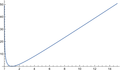
Figure 1: Plot of the function $G$ in (3.2).

Therefore, the function $\Psi$ appears as a strictly increasing function of the non-negative quantities

$${\bf h}(z,w),\qquad\sqrt{\frac{y_{1}}{x_{1}}}+\sqrt{\frac{x_{1}}{y_{1}}}-2,$$ (3.6)

with zero minimum at

$$\bigg{(}{\bf h}(z,w),\sqrt{\frac{y_{1}}{x_{1}}}+\sqrt{\frac{x_{1}}{y_{1}}}-2\bigg{)}=(1,0).$$ (3.7)

Remark 3.1.

Solving (3.7) for $w=(T,y)$, we obtain

$$\begin{cases}y_{1}=x_{1},\\ y_{2}=x_{2}+(T-t)x_{1},\end{cases}$$ (3.8)

which is coherent with the control problem (1.7)-(1.8). Indeed, a solution to (1.8) for $y=(y_{1},y_{2})$ as above is given by $\omega\equiv 0$, which clearly yields $\Psi(t,x;T,y)=0$.

The computation of the function $G$ in (3.2) requires the numerical inversion of trigonometric functions. This makes the use of $\Psi$ numerically challenging, especially in regards to the computation of numerical integrals of the type

$$\int_{x\prec y}e^{-\frac{\Psi(t,x;T,y)}{2}}f(y)dy,$$ (3.9)

which are in turn related to the evaluation of arithmetic Asian options (see (1.46)). For this reason, we look for an expansion of the function $G$ that makes the numerical computation of $\Psi$ more manageable. We would also like such expansion to preserve the asymptotic properties of $G$ as $\eta$ tends to $0^{+}$ and $+\infty$.

We introduce the following

Definition 3.2.

For any $N\in{\mathbb{N}}$ with $N\geq 2$, we define the $N$-th order expansion of $\Psi$ as

$$\Psi_{N}(z,w):=\frac{4}{{\sigma}^{2}(T-t)}\bigg{[}{\bf h}(z,w)\bigg{(}\sqrt{\frac{y_{1}}{x_{1}}}+\sqrt{\frac{x_{1}}{y_{1}}}-2\bigg{)}+\sum_{n=2}^{N}G_{n}\big{(}{\bf h}(z,w)\big{)}\bigg{]},\qquad N\geq 2,$$ (3.10)

where

$$G_{n}(\eta):=a_{n}{\bf 1}_{]1,\infty[}(\eta)\frac{(\eta-1)^{n}}{\eta^{n-1}}+b_{n}{\bf 1}_{]0,1[}(\eta)\frac{(-\log\eta)^{n}}{\big{(}1-\log\eta\big{)}^{n-2}},$$ (3.11)

and where the coefficients $a_{n},b_{n}$ are recursively determined by solving the equations

$$\frac{d^{n}}{d\eta^{n}}G(\eta)\Big{|}_{\eta=1}=\frac{d^{n}}{d\eta^{n}}\sum_{k=2}^{n}G_{k}(\eta)\Big{|}_{\eta=1},\qquad n\geq 1.$$ (3.12)

Before focusing on the convergence results and the asymptotic properties of the approximation $\Psi_{N}$, we discuss some aspects related to its computation. We first point out that the functions $G_{n}$ are written in terms of elementary functions. Therefore, the numerical evaluation of $\Psi_{N}$ is straightforward save computing the coefficients $a_{n},b_{n}$ in (3.11). In regard to this matter, the characterization of the coefficients in Proposition 3.3 below comes in handy. For the sake of completeness, the first $38$ coefficients $a_{n},b_{n}$ are reported in Table 1.

$n$	$a_{n}$	$b_{n}$
2	3	3
3	0.6	-0.6
4	0.205714	-0.444286
5	0.0891429	-0.322
6	0.044144	-0.227237
7	0.0238419	-0.15493
8	0.0136883	-0.100762
9	0.00822413	-0.0610761
10	0.00511786	-0.0328045
11	0.00327527	-0.0133935
12	0.00214449	-0.00074011
13	0.00143104	0.00686845
14	0.0009704	0.0108089
15	0.000667139	0.0121717
16	0.00046414	0.0118058
17	0.000326287	0.0103592
18	0.000231492	0.00831401
19	0.000165581	0.00601859
20	0.000119303	0.00371439
21	0.0000865255	0.00155955
22	0.0000631266	-0.000351322
23	0.0000463045	-0.00197063
24	0.0000341329	-0.00328434
25	0.0000252745	-0.00430119
26	0.000018793	-0.00504427
27	0.0000140273	-0.00554463
28	0.0000105073	-0.0058366
29	$7.89662*10^{-}6$	-0.00595453
30	$5.95282*10^{-}6$	-0.00593069
31	$4.50037*10^{-}6$	-0.00579403
32	$3.41143*10^{-}6$	-0.00556962
33	$2.59248*10^{-}6$	-0.00527856
34	$1.97478*10^{-}6$	-0.00493825
35	$1.5076*10^{-}6$	-0.00456279
36	$1.15335*10^{-}6$	-0.00416351
37	$8.84092*10^{-}7$	-0.00374953
38	$6.78961*10^{-}7$	-0.00332826

Table 1: Values of the coefficients $a_{n},b_{n}$ up to $n=38$.

Proposition 3.3.

For any $n\in{\mathbb{N}}$ with $n\geq 2$, the coefficients $a_{n},b_{n}$ in (3.11) equal to

$$a_{n} =(-1)^{n}\bigg{(}\beta_{n}+\beta_{n-1}-\frac{2}{n!}\sum_{h=0}^{n}\frac{(-1)^{h}(2h)!}{(1-2h)(h!)4^{h}}B_{n,h}\big{(}c_{1},2!c_{2},\cdots,(n-h+1)!c_{n-h+1}\big{)}\bigg{)},$$ (3.13)

$$b_{n} =d_{n-2}-2d_{n-1}+d_{n}+2(e_{n-2}-2e_{n-1}+e_{n}-f_{n-2}+2f_{n-1}-f_{n}),$$ (3.14)

with

$$c_{n} =\beta_{n}+2\beta_{n-1}+\beta_{n-2},$$ (3.15)

$$d_{n} =\frac{1}{n!}\sum_{h=1}^{n}L(n,h)\sum_{k=1}^{h}\beta_{k}k!{h\brace k},$$ (3.16)

$$e_{n} =\frac{1}{n!}\sum_{h=1}^{n}(-1)^{h}L(n,h),\qquad\widetilde{e}_{n}=\frac{1}{n!}\sum_{h=1}^{n}(-2)^{h}L(n,h),$$ (3.17)

$$f_{n} =\frac{1}{n!}\sum_{h=1}^{n}\frac{(-1)^{h}(2h)!}{(1-2h)(h!)4^{h}}B_{n,h}\big{(}d_{1}+\widetilde{e}_{1},2!(d_{2}+\widetilde{e}_{2}),\cdots,(n-h+1)!(d_{n-h+1}+\widetilde{e}_{n-h+1})\big{)},$$ (3.18)

and

$${\beta}_{-1}={\beta}_{0}=0,\qquad{\beta}_{1}=6,\qquad{\beta}_{k}=-\frac{6^{k}}{k!}\sum_{h=1}^{k-1}h!b_{h}B_{k,h}\bigg{(}\frac{1}{3!},\frac{2!}{5!},\cdots,\frac{(k-h+1)!}{[2(k-h+1)+1]!}\bigg{)},\ k\geq 2.$$ (3.20)

Above, the functions $B_{k,h}$ represent the exponential Bell polynomials, $L(n,h)$ denote the Lah numbers, and ${h\brace k}$ the Stirling numbers of the second kind.

Proof.

We first prove (3.13). By the change of variable $\xi:=\frac{\eta-1}{\eta}$, we obtain that (3.12) is equivalent to

$$\frac{1}{n!}\frac{d^{n}}{d\xi^{n}}F(\xi)\Big{|}_{\xi=0}=\frac{1}{n!}\frac{d^{n}}{d\xi^{n}}\sum_{k=2}^{n}a_{k}\xi^{k}\Big{|}_{\xi=0}=a_{n},\qquad n\geq 2,$$ (3.21)

where

$$F(\xi):=(1-\xi)G\Big{(}\frac{1}{1-\xi}\Big{)}=2-2\sqrt{1+(1-\xi)^{2}g^{-1}\left(1-\xi\right)}+(1-\xi)g^{-1}\left(1-\xi\right),\qquad|\xi|<<1.$$ (3.22)

We now go on to compute the power series of $F$ at $\xi=0$. Denoting by $({\beta}_{n})_{n\in\mathbb{N}_{0}}$ the coefficients of the powers series of $g^{-1}$ in $1$, a direct application of Faà di Bruno formula yields

$${\beta}_{0} =0,$$ (3.23)

$${\beta}_{1} =\big{(}{g^{\prime}(0)}\big{)}^{-1},$$ (3.24)

$$n!{\beta}_{n} =-\big{(}{g^{\prime}(0)}\big{)}^{-n}\sum_{h=1}^{n-1}h!{\beta}_{h}B_{n,h}\big{(}g^{\prime}(0),g^{\prime\prime}(0),\cdots,g^{(n-h+1)}(0)\big{)},\qquad n\geq 2,$$ (3.25)

where $B_{n,h}$ represent the exponential Bell polynomials. Note now that, by (3.51), we obtain

$$g^{(n)}(0)=\frac{n!}{(2n+1)!},\qquad n\in{\mathbb{N}}_{0},$$ (3.26)

which yields (3.20). Thus we obtain

$$(1-\xi)g^{-1}(1-\xi) =\sum_{n=1}^{\infty}(-1)^{n}(\beta_{n}+\beta_{n-1})\xi^{n},$$ (3.27)

$$(1-\xi)^{2}g^{-1}(1-\xi) =\sum_{n=1}^{\infty}(\beta_{n}+2\beta_{n-1}+\beta_{n-2})\xi^{n},$$ (3.28)

for any $\xi$ close to $0$. Eventually, applying once more Faà di Bruno formula, together with

$$\sqrt{1+x}=1+\sum_{n=1}^{\infty}\frac{(-1)^{n}(2n)!}{(1-2n)(n!)^{2}4^{n}}x^{n},\qquad|x|<<1,$$ (3.29)

yield (3.21) with $a_{n}$ as given by (3.13).

To prove (3.14) we use an analogous argument. By the change of variable $\xi:=\frac{-\log\eta}{1-\log\eta}$, we obtain that (3.12) is equivalent to

$$\frac{1}{n!}\frac{d^{n}}{d\xi^{n}}F(\xi)\Big{|}_{\xi=0}=\frac{1}{n!}\frac{d^{n}}{d\xi^{n}}\sum_{k=2}^{n}b_{k}\xi^{k}\Big{|}_{\xi=0}=b_{n},\qquad n\geq 2,$$ (3.30)

where

$$F(\xi):=(1-\xi)^{2}G\Big{(}e^{\frac{\xi}{\xi-1}}\Big{)}=(1-\xi)^{2}\Big{(}2e^{\frac{\xi}{\xi-1}}-2\sqrt{e^{\frac{2\xi}{\xi-1}}+g^{-1}\big{(}e^{\frac{\xi}{1-\xi}}\big{)}}+g^{-1}\big{(}e^{\frac{\xi}{1-\xi}}\big{)}\Big{)},\qquad|\xi|<<1.$$ (3.31)

By applying now Faà di Bruno formula we obtain

$$e^{\frac{\xi}{\xi-1}}-1 =\sum_{n=1}^{\infty}\frac{\xi^{n}}{n!}\sum_{h=1}^{n}B_{n,h}\big{(}-1,-2!,\cdots,-(n-h+1)!\big{)}=\sum_{n=1}^{\infty}\frac{\xi^{n}}{n!}\sum_{h=1}^{n}(-1)^{h}\binom{n-1}{h-1}\frac{n!}{h!}=\sum_{n=1}^{\infty}e_{n}{\xi^{n}},$$ (3.32)

$$e^{\frac{2\xi}{\xi-1}}-1 =\sum_{n=1}^{\infty}\frac{\xi^{n}}{n!}\sum_{h=1}^{n}B_{n,h}\big{(}-2,-2\cdot 2!,\cdots,-2\cdot(n-h+1)!\big{)}=\sum_{n=1}^{\infty}\widetilde{e}_{n}{\xi^{n}},$$ (3.33)

$$g^{-1}\big{(}e^{\frac{\xi}{1-\xi}}\big{)} =\sum_{n=1}^{\infty}\frac{\xi^{n}}{n!}\sum_{h=1}^{n}B_{n,h}\big{(}1,2!,\cdots,(n-h+1)!\big{)}\sum_{k=1}^{h}k!\beta_{k}B_{n,k}(1,\cdots,1)=\sum_{n=1}^{\infty}{d}_{n}{\xi^{n}},$$ (3.34)

for any $\xi$ close to $0$, where $d_{n},e_{n},\widetilde{e}_{n}$ are as in (3.16)-(3.17). Eventually, applying again Faà di Bruno formula together with (3.29) yield (3.30) with $b_{n}$ as in (3.14). ∎

We now address both point-wise and asymptotic convergence of $\Psi_{N}$ to $\Psi$. Concerning the former one, the desired result would be

$$\sum_{n=2}^{N}G_{n}(\eta)\to G(\eta)\qquad\text{as }N\to+\infty,$$ (3.35)

for any $\eta>0$, which would in turn imply

$$\Psi_{N}(z,w)\to\Psi(z,w)\qquad\text{as }N\to\infty,$$ (3.36)

for any $z,w\in{\mathbb{R}}\times D$ with $z\prec w$. However, unfortunately, we were able to provide a rigorous proof of (3.35) only for $\eta>1$ (see Theorem 3.4 below). Despite of this, we point out that strong numerical evidence suggests that (3.35) is satisfied also for $\eta\in]0,1[$. To support this claim, in Figure 2 we compare the plot of the truncated series $\sum_{n=2}^{N}G$ with that of $G$, for different values of $N$.

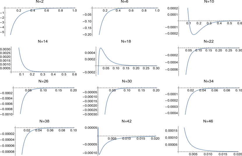
Figure 2: Plot of the difference $G(\eta)-\sum_{n=2}^{N}G_{n}(\eta)$, with $G_{n}$ as in Definition 3.2, for values of $\eta$ close to $0$.

Theorem 3.4.

For any $\eta>1$ the limit (3.35) holds true.

The proof of Theorem 3.4 is deferred until Section 3.1.

We now turn our attention to the asymptotic convergence. By definition of $g$ we can easily obtain

$$g^{-1}(h)\sim\log^{2}h\qquad\text{ as }h\to+\infty,$$ (3.37)

where, as already stated in the introduction, we adopted the notation

$$f\sim g\Leftrightarrow\frac{f}{g}\longrightarrow 1.$$ (3.38)

The definition of $G$ together with (3.37) then yield

$$G(\eta)\sim 4\eta\qquad \text{as }\eta\to+\infty,$$ (3.39)

$$G(\eta)\sim\log^{2}\eta\qquad \text{as }\eta\to 0^{+}.$$ (3.40)

The idea behind the approximation $\Psi_{N}$ is to expand the function $G$ by means of suitable basis functions so as to obtain

$${\sum_{n=2}^{N}G_{n}(\eta)}\sim\eta\sum_{n=2}^{N}a_{n}\qquad \text{as }\eta\to\infty,$$ (3.41)

$${\sum_{n=2}^{N}G_{n}(\eta)}\sim(\log^{2}\eta)\sum_{n=2}^{N}b_{n}\qquad \text{as }\eta\to 0^{+}.$$ (3.42)

Indeed, the latter easily stem from

$$\frac{(\eta-1)^{n}}{\eta^{n-1}} \sim\eta\qquad\text{as }\eta\to+\infty,$$ (3.43)

$$\frac{(-\log\eta)^{n}}{\big{(}1-\log\eta\big{)}^{n-2}} \sim\log^{2}\eta\qquad\text{as }\eta\to 0^{+}.$$ (3.44)

Ideally, we would like to show that

$$\lim_{N\to\infty}\sum_{n=2}^{N}a_{n}= 4,$$ (3.45)

$$\lim_{N\to\infty}\sum_{n=2}^{N}b_{n}= 1,$$ (3.46)

which means the asymptotic behavior of $\sum_{n=2}^{N}G_{n}(\eta)$ converges to the asymptotic behavior of $G(\eta)$ as $\eta$ tends to $0^{+}$ and $+\infty$. Note that this property is in general not granted for convergent expansions. We start by considering the case $\eta>1$. In Corollary 3.5 below, we show that (3.45) is satisfied provided that the coefficients $a_{n}$ are all positive. Unfortunately, we were not able to rigorously prove the positiveness of the coefficients $a_{n}$, thought the numerical values reported in Table 1 strongly support this conjecture.

Corollary 3.5.

Under the assumption that the coefficients $(a_{n})_{n\geq 2}$ are all positive, the limit (3.45) holds true.

Proof.

Let $\bar{a}:=\lim_{N\to\infty}\sum_{n=2}^{N}a_{n}$ and assume $\bar{a}<4$. By definition (3.11), and by (3.39), there exists $\bar{\eta}>1$ such that

$$\sum_{n=2}^{N}G_{n}(\bar{\eta})<\bar{a}\bar{\eta}<\frac{\bar{a}+4}{2}\bar{\eta}<G(\bar{\eta}),\qquad N\geq 2.$$ (3.47)

This violates Theorem 3.4 and yields a contradiction. Therefore, we have $\bar{a}\geq 4$.

Assume now that $\bar{a}>4$. Then there exits $\bar{N}$ such that

$$\sum_{n=2}^{\bar{N}}a_{n}>\frac{\bar{a}+4}{2}.$$ (3.48)

On the other hand, the positiveness of the coefficients $a_{n}$, together with (3.39) and (3.42), implies that there exists $\bar{\eta}>1$ such that

$$\sum_{n=2}^{N}G_{n}(\bar{\eta})>\sum_{n=2}^{\bar{N}}G_{n}(\bar{\eta})>\frac{\bar{a}+4}{2}\bar{\eta}>G(\bar{\eta}),\qquad N>\bar{N},$$ (3.49)

which again violates Theorem 3.4 and yields a contradiction. This proves that $\bar{a}\leq 4$ and concludes the proof.

∎

For $\eta\in]0,1[$ the situation is less clear. On the one hand, the values in Table 1 suggests that the sign of the coefficients $b_{n}$ oscillates as $n$ grows, and thus we cannot rely on the positiveness (or negativeness) of the coefficients $b_{n}$ to infer (3.46). On the other hand, the plot in Figure 3 shows that $\sum_{n=2}^{N}b_{n}$ is close to $1$ for (not too) large values of $N$. Unfortunately, the numerical complexity of the representation (3.14) makes it very difficult to compute the summation above for larger values of $N$. Therefore, the question whether (3.46) is actually true remains open.

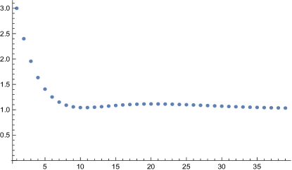
Figure 3: Plot of the sum $\sum_{n=2}^{N}b_{n}$ for $N$ up to $40$.

3.1 Proof of Theorem 3.4

This section is devoted to the proof of Theorem 3.4, which is preceded by some preliminary results. Hereafter, for any $z\in\mathbb{C}$ and $\delta>0$, we denote by $B_{\delta}(z)$ the complex ball centered at $z$ with radius $\delta$.

Lemma 3.6.

The function $g$ defined by (2.14) is holomorphic on $\mathbb{C}$, and

$$g^{\prime}(z)\neq 0,\qquad z\in{B_{\pi^{2}}(0)}.$$ (3.50)

Furthermore, the restriction of $g$ to $\partial B_{\pi^{2}}(0)$ is a homeomorphism, and its image surrounds $B_{1}(1)$.

Proof.

Owing to the Taylor series expansion of $\sinh z$ around $z=0$, we directly obtain

$$g(z)=\sum_{n=0}^{\infty}\frac{z^{n}}{(2n+1)!},\qquad r\in\mathbb{C},$$ (3.51)

which shows that $g$ is holomorphic on $\mathbb{C}$.

We now prove that $g^{\prime}\neq 0$ on $B_{\pi^{2}}(0)$. Differentiating (2.14) we obtain

$$g^{\prime}(z)=\frac{f(\sqrt{z})}{2z^{{3}/{2}}},\qquad z\in\mathbb{C},$$ (3.52)

where

$$f(z):=z\cosh z-\sinh z=\sum_{n=1}^{\infty}\frac{2n}{(2n+1)!}z^{2n+1}.$$ (3.53)

Therefore, owing to the fact that $g^{\prime}(0)=1/6$ (by (3.51)), and to $f(\bar{z})=\overline{f(z)}$, we have that (3.50) is equivalent to

$$f(z)\neq 0,\qquad z\in\widetilde{B}_{\pi}(0)\setminus\{0\},$$ (3.54)

where

$$\widetilde{B}_{\pi}(0):=\{x+iy\in{B}_{\pi}(0):x,y\geq 0\}.$$ (3.55)

We first observe, that

$$f(x)\neq 0,\qquad x\in{\mathbb{R}},\ x\neq 0,$$ (3.56)

which follows directly from the series representation in (3.53). Finally, a direct computation shows that

$$|f(z)|^{2} =\frac{1}{2}\Big{(}\left(x^{2}+y^{2}-1\right)\cos(2y)+\left(x^{2}+y^{2}+1\right)\cosh(2x)-2x\sinh(2x)-2y\sin(2y)\Big{)}$$ (3.57)

$$>|f(x)|^{2}$$ (3.58)

for any $z=x+iy\in\widetilde{B}_{\pi}(0)$ with $y>0$. This, together with (3.56), proves (3.54).

We now prove that $g|_{\partial B_{\pi^{2}}(0)}$ is a homeomorphism: it is enough to show that it is injective. Owing to

$$\overline{g(z)}=g(\overline{z}),\qquad z\in\mathbb{C},$$ (3.59)

the latter property can be proved by checking that the function $\theta\mapsto|\sinh(\pi e^{i\theta})|$ is strictly decreasing on $[0,\pi/2]$, and that the imaginary part of $e^{-i\theta}\sinh(\pi e^{i\theta})$ is strictly positive for $\theta\in]0,\pi/2[$. We omit the details for brevity.

Finally, we prove that the image of $g|_{\partial B_{\pi^{2}}(0)}$ surrounds $B_{1}(1)$. Owing again to (3.59), it is enough to prove that

$$\Big{|}\frac{\sinh(\pi e^{i\theta})}{\pi e^{i\theta}}-1\Big{|}\geq 1,\qquad\theta\in[0,\pi/2].$$ (3.60)

We have

$$\Big{|}\frac{\sinh(\pi e^{i\theta})}{\pi e^{i\theta}}-1\Big{|}=\frac{1}{\pi}\Big{|}\sum_{n=1}^{\infty}\frac{(\pi e^{i\theta})^{2n+1}}{(2n+1)!}\Big{|}\geq\frac{1}{\pi}|I_{1}(\theta)-I_{2}|,$$ (3.61)

with

$$I_{1}(\theta)=\Big{|}\sum_{n=1}^{3}\frac{(\pi e^{i\theta})^{2n+1}}{(2n+1)!}\Big{|},\qquad I_{2}=\sum_{n=4}^{\infty}\frac{\pi^{2n+1}}{(2n+1)!}.$$ (3.62)

Now, it is not difficult to prove that there exists $\varsigma>0$ such that

$$I_{1}(\theta)>\varsigma+\pi>I_{2}+\pi,\qquad\theta\in[0,\pi/2],$$ (3.63)

which proves (3.60). ∎

We are now in the position to prove Theorem 3.4.

Proof of Theorem 3.4.

By the change of variable $\xi:=\frac{\eta-1}{\eta}$, it suffices to prove

$$F(\xi):=(1-\xi)G\Big{(}\frac{1}{1-\xi}\Big{)}=\sum_{n=2}^{\infty}a_{n}\xi^{n},\qquad\xi\in]-1,1[.$$ (3.64)

We prove (3.64) by showing that $F$ is holomorphic on $B_{1}(0)$. Explicitly, we have

$$F(\xi):=(1-\xi)\bigg{(}\frac{2}{1-\xi}-2(1-\xi-2/\pi)\sqrt{\frac{(1-\xi)^{-2}+g^{-1}\left(1-\xi\right)}{(1-\xi-2/\pi)^{2}}}+g^{-1}\left(1-\xi\right)\bigg{)}.$$ (3.65)

Lemma 3.6 combined with Lemma A.1 imply that $g|_{B_{\pi^{2}}(0)}$ is a biholomorphism on its image. In particular, the inverse $g^{-1}$ is well defined and holomorphic on $B_{1}(1)$. Setting now

$$f(z):={z^{-2}+g^{-1}(z)},\qquad z\in B_{1}(1),$$ (3.66)

it is straightforward to check that

$$f\Big{(}\frac{2}{\pi}\Big{)}=0=f^{\prime}\Big{(}\frac{2}{\pi}\Big{)}.$$ (3.67)

The first equality above follows directly from (3.4), whereas the second stems from (3.4) together with

$$f^{\prime}(2/\pi)=-2z^{-3}+\frac{2g^{-1}(z)}{\sqrt{1+zg^{-1}(z)}-z}\bigg{|}_{z=2/\pi},\qquad z\in{\mathbb{R}}.$$ (3.68)

It follows that

$$z\mapsto\frac{f(z)}{(z-2/\pi)^{2}}$$ (3.69)

is holomorphic on $B_{1}(1)$. it is also possible to observe that $f\big{(}B_{1}(1)\big{)}$ does not contain non-negative real numbers, which finally yields holomorphicity of $F$ on $B_{1}(0)$.

∎

4 Yosida’s parametrix construction

For the sake of clarity, before dwelling on the details of our extension of Yosida’s parametrix method, we outline the general parametrix construction of the fundamental solution $p$, for a general choice of the parametrix function.

4.1 General parametrix construction

Consider a given function $H(z;w)$, hereafter referred to as parametrix function, or simply parametrix, which enjoys suitable regularity and boundedness properties, together with the Dirac delta property ii) in Definition 2.2, and such that

$$H(t,x_{1},x_{2};T,y_{1},y_{2})\to 0\qquad\text{as }y_{2}\to x_{2}^{+}.$$ (4.1)

Following the standard approach, we look for $p=p(z;w)$ of the form

$$p(z,w)=H(z,w)+\int_{z\prec\zeta\prec w}H(z;\zeta)\Phi(\zeta;w)d\zeta,\qquad z\prec w.$$ (4.2)

By formally applying Point i) in Definition 2.2, we obtain

$$0=\mathscr{L}p(z,w)=\mathscr{L}H(z,w)+\mathscr{L}\int_{z\prec\zeta\prec w}H(z;\zeta)\Phi(\zeta;w)d\zeta$$ (4.3)

(owing to the Dirac delta property $$H(t,x;t,\xi)=\delta_{x}$$ and to (4.1))

$$=\mathscr{L}H(z,w)+\int_{z\prec\zeta\prec w}\mathscr{L}H(z;\zeta)\,\Phi(\zeta;w)d\zeta-\Phi(z,w),$$ (4.4)

which yields

$$\Phi(z,w)=\mathscr{L}H(z,w)+\int_{z\prec\zeta\prec w}\mathscr{L}H(z;\zeta)\,\Phi(\zeta;w)d\zeta,\qquad z\prec w.$$ (4.5)

Now by Picard iteration we look for a solution to (4.5) of the form

$$\Phi(z;\zeta)=\sum_{n=0}^{\infty}K_{n}(z;\zeta),\qquad z\prec w,$$ (4.6)

where the functions $K_{n}$ are defined through the recursion

$$K_{0}(z;w)=\mathscr{L}H(z;w), K_{n}(z;w)=\int_{z\prec\zeta\prec w}\mathscr{L}H(z;\zeta)K_{n-1}(\zeta,w)d\zeta,\qquad n\geq 1.$$ (4.7)

In order for the construction above to be formalized, one needs to find a parametrix $H$ satisfying suitable estimates so that:

• the series in (4.6) is convergent;

• the properties i) and ii) of Definition 2.2 can be verified.

Furthermore, as a by-product of (4.2) and of the estimates for $H$ and $\Phi$, one can prove bounds for $p$ and its derivatives. In our case, thanks to a specific choice of $H$, we will be able to prove the estimates in Theorem 1.1 and Theorem 1.2.

4.2 Generalized Yosida’s parametrix

Following Yoshida [37], we introduce our parametrix $H$ in two steps. We first define a pre-parametrix $H_{1}$ as a function having the expected asymptotic behavior both away from the pole, and close to the pole. As we will see, the function $H_{1}$ is not suitable to define the integrals appearing in (4.7). Hence, in the second step, we introduce a correction term $\bf{u}$ that makes the functions $K_{n}$’s well defined if we use $H:={\bf u}H_{1}$ as a parametrix.

Hereafter throughout the whole section we will set $\sigma=1$ without loss of generality (see Remark 2.5). For any $z=(t,x),w=(T,y)\in{\mathbb{R}}\times D$ with $z\prec w$, define the pre-parametrix $H_{1}$ as in (1.38). Explicitly,

$$H_{1}(z;w)=\frac{\sqrt{12}}{2\pi(T-t)^{2}y_{1}^{2}}e^{-\frac{1}{2}\Psi(z;w)}.$$ (4.8)

The idea behind this definition is the following. On one hand, the cost function $\Psi$ at the exponential is supposed to provide the exact asymptotic behavior of the fundamental solution away from the pole. On the other hand, the square root of the determinant of ${\bf C}$ in the denominator yields the same singular behavior near the pole as the fundamental solution of the frozen operator

$$\widetilde{\mathscr{L}}_{y}={\partial_{t}+x_{1}\partial_{x_{2}}}+\frac{y_{1}^{2}}{2}\partial_{x_{1}x_{1}},\qquad(t,x_{1},x_{2})\in{\mathbb{R}}^{3}.$$ (4.9)

In practice, this specific choice for the denominator ensures that $H_{1}(z,w)$ enjoys the Dirac Delta property ii) in Definition 2.2. The exact statement for this is in Proposition 4.4 below.

Now, if we were to choose $H_{1}$ as a parametrix, the first step towards proving the convergence of the series (4.6) would be to bound $\mathscr{L}H_{1}$ from above. To do so, one first computes

$$\partial_{t}H_{1} =\bigg{(}\frac{2}{T-t}-\frac{1}{2}\partial_{t}\Psi\bigg{)}H_{1},$$ (4.10)

$$\partial_{x_{1}}H_{1} =-\frac{1}{2}\big{(}\partial_{x_{1}}\Psi\big{)}H_{1},$$ (4.11)

$$\partial_{x_{2}}H_{1} =-\frac{1}{2}\big{(}\partial_{x_{2}}\Psi\big{)}H_{1},$$ (4.12)

$$\partial_{x_{1}x_{1}}H_{1} =\bigg{(}\frac{1}{4}\big{(}\partial_{x_{1}}\Psi\big{)}^{2}-\frac{1}{2}\partial_{x_{1}x_{1}}\Psi\bigg{)}H_{1},$$ (4.13)

and obtains

$$\mathscr{L}H_{1}(z;w)=\bigg{(}\Big{(}\frac{x_{1}}{2}\partial_{x_{1}}\Psi(z;w)\Big{)}^{2}-Y\Psi(z;w)+f(z,w)\bigg{)}H_{1}(z;w),$$ (4.14)

with

$$f(t,x;T,y):=\frac{2}{T-t}-\frac{x_{1}^{2}\partial_{x_{1}x_{1}}\Psi(t,x;T,y)}{4}.$$ (4.15)

At first glance, a twofold problem appears:

• the function $f(z,w)$ is singular of order $\frac{1}{T-t}$;

• the functions

  $$\Big{(}\frac{x_{1}}{2}\partial_{x_{1}}\Psi(z;w)\Big{)}^{2}\quad\text{and}\quad Y\Psi(z;w)$$ (4.16)

  are singular of order $\frac{1}{(T-t)^{2}}$.

In light of the space-time convolutions that define the terms $K_{n}$ in (4.7), the presence of these singular terms seems to undermine the construction using $H_{1}$. However, the next lemma shows that the singular terms of order $\frac{1}{(T-t)^{2}}$ cancel each other out.

Lemma 4.1 (HJB equation).

For any $w=(T,y)\in{\mathbb{R}}\times D$, the function $\Psi(\cdot,\cdot;T,y)$ satisfies

$$Y\Psi(z;w)=\Big{(}\frac{x_{1}}{2}\partial_{x_{1}}\Psi(z;w)\Big{)}^{2},\qquad z=(t,x)\in{\mathbb{R}}\times D,\ z\prec w.$$ (4.17)

Furthermore, the optimal control $\omega$ for the problem (1.7)-(1.8) satisfies

$$\omega(s)=-\frac{\gamma_{1}(s)}{2}\partial_{\gamma_{1}}\Psi\big{(}s,\gamma(s);w\big{)},\qquad s\in[t,T].$$ (4.18)

The proof is deferred until Appendix B.

By applying (4.17) to (4.14) we obtain

$$\mathscr{L}H_{1}(z;w)=f(z,w)H_{1}(z;w).$$ (4.19)

In order to get rid of the singularity of order $\frac{1}{T-t}$, we define the parametrix $H$ as

$$H(z;w):=H_{1}(z;w){\bf u}(z;w),$$ (4.20)

where ${\bf u}$ is a regular function, suitably chosen so as to obtain a uniform bound for $\mathscr{L}H(z,w)$. By (4.19) we obtain

$$\mathscr{L}H(z;w) =\Big{(}{f(z,w){\bf u}(z;w)-g(z,w)\partial_{x_{1}}{\bf u}(z;w)}+\mathscr{L}{\bf u}(z;w)\Big{)}H_{1}(z;w)$$ (4.21)

$$=\Big{(}\big{(}Y-g(z;w)\partial_{x_{1}}+f(z,w)\big{)}{\bf u}(z;w)+\frac{x_{1}^{2}}{2}\partial_{x_{1}x_{1}}{\bf u}(z;w)\Big{)}H_{1}(z;w),$$ (4.22)

with $f$ as given in (4.15) and

$$g(z;w):=\frac{x_{1}^{2}}{2}\partial_{x_{1}}\Psi(z;w).$$ (4.23)

The idea is then to find ${\bf u}$ that verifies

$$\big{(}Y-g(z;w)\partial_{x_{1}}\big{)}{\bf u}(z;w)+f(z;w){\bf u}(z;w)=0,\qquad z\prec w,$$ (4.24)

and such that

$$\frac{x_{1}^{2}}{2}\partial_{x_{1}x_{1}}{\bf u}(z;w)$$ (4.25)

is bounded with respect to $T-t$. We also impose that that the initial condition

$${\bf u}(w;w)=1$$ (4.26)

is verified in some sense. Intuitively, the latter is required in order for the Dirac Delta property, as $(T-t)\to 0^{+}$, to be transferred from $H_{1}$ to $H$. We seek a solution to (4.24)-(4.26) by employing the method of the characteristic curves. We have the following crucial

Lemma 4.2.

For any $w=(T,y)\in{\mathbb{R}}\times D$, the integral curves of the vector field

$$z\mapsto Y-g(z,w)\partial_{x_{1}},\qquad z=(t,x)\in{\mathbb{R}}\times D,\ z\prec w,$$ (4.27)

are the optimal curves $\big{(}s,\gamma(s)\big{)}$ for the optimal control problem (1.7)-(1.8) with $\gamma(T)=y$.

Proof.

By (4.18), we have

$$\begin{cases}\dot{\gamma}_{1}(s)=-g\big{(}s,\gamma(s);w\big{)}\\ \dot{\gamma}_{2}(s)=\gamma_{1}(s)\end{cases},\qquad t<s<T,$$ (4.28)

which completes the proof. ∎

Applying now Lemma 4.2, together with the method of the characteristic curves, we find that the solution to (4.24)-(4.26) has to be

$${\bf u}(z;w) :=\exp\bigg{(}\int_{t}^{T}f\big{(}s,\gamma(s);T,y\big{)}ds\bigg{)}$$ (4.29)

$$=\exp\bigg{(}\int_{t}^{T}\Big{[}\frac{2}{T-s}-\frac{\gamma_{1}^{2}(s)\partial_{\gamma_{1}\gamma_{1}}\Psi\big{(}s,\gamma(s);w\big{)}}{4}\Big{]}ds\bigg{)},\qquad z\prec w,$$ (4.30)

where $\gamma$ denotes the optimal trajectory of the control problem (1.7)-(1.8). In the next section we will prove that such ${\bf u}$ is well defined, and that the iterative construction described in Section 4.1 converges to the fundamental solution $p$ of $\mathscr{L}$, with the parametrix function $H$ given by (4.20)-(4.8)-(4.30).

4.3 Convergence of the Picard series and proofs of Theorems 1.1 and 1.2

We prove Theorems 1.1 and 1.2 by estimating the series (4.6) and the integral in (4.2) with $H$ as defined in the previous section, and by proving that $p$ as defined by (4.2) is indeed the fundamental solution of $\mathscr{L}$.

We start with the following two propositions, whose proofs are deferred until Sections 4.3 and 4.4.

Proposition 4.3.

The function ${\bf u}$ given by (4.30) is well defined and we have

$${\bf u}(z;w)=v\Big{(}{4}\,g^{-1}\Big{(}\frac{1}{{\bf h}(z;w)}\Big{)}\Big{)},$$ (4.31)

with

$$v(\eta)=\begin{cases}\frac{|\eta|}{2\sqrt{3\sqrt{\eta}\sinh(\sqrt{\eta})-6\cosh(\sqrt{\eta})+6}},\quad&\eta\in\,]-4\pi^{2},+\infty[\,\setminus\{0\}\\ 1,\quad&\eta=0\end{cases}.$$ (4.32)

Furthermore, the function ${\bf u}(\cdot;\zeta)$ is smooth and solves (4.24).

Finally there exists a universal constant $\kappa>0$ such that

$$\kappa^{-1}{\bf 1}_{]0,1]}\big{(}{\bf h}(z;w)\big{)}{\bf h}(z;w)\leq|{\bf u}(z;w)|\leq\kappa\big{(}\sqrt{{\bf h}}+{\bf h}\big{)}(z;w),$$ (4.33)

$$\big{|}{x_{1}^{2}}\partial_{x_{1}x_{1}}{\bf u}(z;w)\big{|}\leq\kappa\,\sqrt{{\bf h}(z;w)},$$ (4.34)

for any $z=(t,x),w=(T,y)\in{\mathbb{R}}\times D$ with $z\prec w$.

The next statement is crucial in order to check that parametrix $H$ enjoys the Dirac delta property ii) in Definition 2.2.

Proposition 4.4.

For any function $\widetilde{v}\in C({\mathbb{R}}^{+})$ bounded by a power function, such that $\widetilde{v}(1)=1$, we have

$$\lim_{T\to 0^{+}}\ \int\limits_{(1,0)\prec\xi}\widetilde{v}\big{(}{\bf h}({\bf 1}_{\mathbb{G}};T,\xi)\big{)}H_{1}({\bf 1}_{\mathbb{G}};T,\xi)\varphi(\xi)d\xi=\varphi(1,0),\qquad\varphi\in C_{b}(D).$$ (4.35)

In order to carry on with the convergence analysis it is essential to provide bounds for the integrals in (4.7) and (4.2). In light of estimates (4.34)-(4.33), such bounds are consequences of the following

Key Inequalities 4.5.

Let ${\bf h}$ be as defined in (4.34) and $\widetilde{g}$ be the function

$$\widetilde{g}(h)=\sqrt{h}+h.$$ (4.36)

For any $\tau>0$, there exists a constant $C_{\tau}>0$ such that

$$\int_{x\prec\xi\prec(1,0)}\sqrt{{\bf h}(z;s,\xi)}H_{1}(z;s,\xi)\sqrt{{\bf h}(s,\xi;{\bf 1}_{\mathbb{G}})}H_{1}(s,{\xi};{\bf 1}_{\mathbb{G}})d\xi \leq C_{\tau}\,\sqrt{{\bf h}(z;{\bf 1}_{\mathbb{G}})}H_{1}(z,{\bf 1}_{\mathbb{G}}),\qquad s\in]t,0[,\qquad\qquad$$ (4.37)

$$\int_{x\prec\xi\prec(1,0)}\widetilde{g}\big{(}{{\bf h}(z;s,\xi)}\big{)}H_{1}(z;s,\xi)\widetilde{g}\big{(}{{\bf h}(s,\xi;{\bf 1}_{\mathbb{G}})}\big{)}H_{1}(s,{\xi};{\bf 1}_{\mathbb{G}})d\xi \leq C_{\tau}\,\widetilde{g}\big{(}{{\bf h}(z;{\bf 1}_{\mathbb{G}})}\big{)}H_{1}(z,{\bf 1}_{\mathbb{G}}),\qquad s\in]t,0[,\qquad$$ (4.38)

for any $z=(t,x)\in{\mathbb{R}}\times D$ such that $z\prec{\bf 1}_{\mathbb{G}}$ and $t>-\tau$.

As already pointed out in the introduction, at the current stage we were not able to provide a proof for the bounds in Key Inequalities 4.5. In Section 4.5 we collect a considerable amount of numerical evidence in favor of the claim that these estimates hold true. This makes us comfortable in conjecturing their validity. However, given that a rigorous proof is currently missing, the Key Inequalities 4.5 are part of the hypotheses of Theorems 1.1 and 1.2.

Theorem 4.6.

Assume that Key Inequalities 4.5 hold true. Then the series in (4.6) converges, and for any $\tau>0$ there exists a positive constant $C>0$, only dependent on $\tau$, such that

$$\Big{|}\int_{z\prec\zeta\prec w}H(z;\zeta)\Phi(\zeta;w)d\zeta\Big{|}\leq C(T-t)\big{(}\sqrt{{\bf h}(z;w)}+{\bf h}(z;w)\big{)}H_{1}(z,w),$$ (4.39)

for any $z=(t,x),\zeta=(T,w)\in{\mathbb{R}}\times D$ with $z\prec w$ and $T-t<\tau$.

Furthermore, the function $p$ given by (4.2) is the fundamental solution of $\mathscr{L}$ with $\sigma=1$.

Before proving Theorem 4.6, we prove Theorems 1.1 and 1.2, which are straightforward consequences of Theorem 4.6.

Proof of Theorem 1.1.

In light of Remark 2.5, it is not restrictive to assume $\sigma=1$. Thus the bound (1.12) stems from Theorem 4.6, in particular by applying the estimates (4.33)-(4.39) to (4.2). ∎

Proof of Theorem 1.2.

In light of Remark 2.5, it is not restrictive to assume $\sigma=1$ and $w={\bf 1}_{\mathbb{G}}$. To ease notation we remove the explicit dependence on ${\bf 1}_{\mathbb{G}}$ in the functions below.

All the following inequalities are meant for any $z=(t,x)\in\,]-1,0[\,\times D$ such that

$$\frac{1}{\kappa}\leq\frac{\sqrt{x_{1}}}{-x_{2}}\leq\kappa.$$ (4.40)

By Theorem 4.6 we obtain

$$p(t,x)\geq H(t,x)-\bigg{|}\int_{(t,x)\prec\zeta\prec w}H(t,x;\zeta)\Phi(\zeta)d\zeta\bigg{|}\geq H(t,x)-C(-t)\big{(}\sqrt{{\bf h}}+{\bf h}\big{)}(t,x)H_{1}(t,x),$$ (4.41)

where $C$ is a universal constant independent of any variable. Furthermore, by (4.40), we have

$${\bf h}(t,x)\leq 1,\qquad t\in[-{\kappa}^{-1},0[,$$ (4.42)

and thus (4.41) together with the first equality in (4.33) yield

$$p(t,x) \geq\Big{(}{\bf h}(t,x)-C(-t)\big{(}\sqrt{{\bf h}}+{\bf h}\big{)}(t,x)\Big{)}H_{1}(t,x)$$ (4.43)

$$=\bigg{(}1-C(-t)-C\sqrt{-t}\Big{(}{\frac{-x_{2}}{\sqrt{x_{1}}}}\Big{)}^{1/2}\bigg{)}{\bf h}(t,x)H_{1}(t,x)$$ (4.44)

(by the first inequality in (4.40))

$$\geq\big{(}1-C(-t)-C\sqrt{-t}\sqrt{\kappa}\,\big{)}{\bf h}(t,x)H_{1}(t,x)$$ (4.45)

for any $t\in[-{\kappa}^{-1},0[$. This completes the proof. ∎

We conclude the section with the proof of Theorem 4.6.

Proof of Theorem 4.6.

We first prove convergence of the series in (4.6) and estimate (4.39). In light of (2.17)-(2.19), it is not restrictive to assume $w={\bf 1}_{\mathbb{G}}$. To ease notation we remove the explicit dependence on ${\bf 1}_{\mathbb{G}}$ in the functions below. Furthermore, we will denote by $C_{1},C_{2},\dots$ any positive constant that depends at most on $\tau$.

By Proposition 4.3, in particular by applying (4.24) to (4.22), we obtain

$$\mathscr{L}H(z,\zeta)=\frac{x_{1}^{2}}{2}\partial_{x_{1}x_{1}}{\bf u}(z,\zeta)H_{1}(z,\zeta),\qquad z\prec\zeta.$$ (4.46)

Therefore, by (4.7) and employing (4.34), we obtain

$$|K_{0}(z)|\leq C_{1}\sqrt{{\bf h}(z)}H_{1}(z).$$ (4.47)

In general, by induction we can also prove

$$|K_{n}(z)|\leq C_{2}^{n}C_{1}^{n+1}\frac{(-t)^{n}}{n!}\sqrt{{\bf h}(z)}H_{1}(z)$$ (4.48)

for any $n\in\mathbb{N}_{0}$. Indeed, assuming (4.48) true, we have

$$|K_{n+1}(z)| \leq\frac{C_{2}^{n}C_{1}^{n+1}}{n!}\int_{z\prec\zeta\prec{\bf 1}_{\mathbb{G}}}(-s)^{n}\big{|}\mathscr{L}H(z,\zeta)\big{|}\sqrt{{\bf h}(\zeta)}H_{1}(\zeta)d\zeta$$ (4.49)

(by (4.46)-(4.34))

$$\leq\frac{C_{2}^{n}C_{1}^{n+2}}{n!}\int_{z\prec\zeta\prec{\bf 1}_{\mathbb{G}}}(-s)^{n}\sqrt{{\bf h}(z;\zeta)}H_{1}(z;\zeta)\sqrt{{\bf h}(\zeta)}H_{1}(\zeta)d\zeta$$ (4.50)

(by (4.37))

$$\leq\frac{C_{2}^{n+1}C_{1}^{n+2}}{n!}\int_{t}^{0}(-s)^{n}ds\,\sqrt{{\bf h}(z)}H_{1}(z)$$ (4.51)

$$\leq C_{2}^{n+1}C_{1}^{n+2}\frac{(-t)^{n+1}}{(n+1)!}\sqrt{{\bf h}(z)}H_{1}(z).$$ (4.52)

Summing over $n$, we obtain that the series in (4.6) converges and that

$$|\Phi(z)|\leq C_{1}\,e^{-C_{1}C_{2}t}\sqrt{{\bf h}(z)}H_{1}(z).$$ (4.53)

This, together with (4.33)-(4.38), yields (4.39).

We now go on to prove the second part of the statement, namely that $p$ as defined by (4.2) is the fundamental solution of $\mathscr{L}$ with $\sigma=1$.

For any $x^{\prime}\in D$ and $t<s$, and for any $\varphi\in C_{b}(D)$, we have

$$\int_{x^{\prime}\prec y}H(t,x^{\prime};T,y)\varphi(y)dy =\int_{x^{\prime}\prec y}{\bf u}(t,x^{\prime};T,y)H_{1}(t,x^{\prime};T,y)\varphi(y)dy$$ (4.54)

(by (2.17)-(2.19))

$$=\int_{x^{\prime}\prec y}{\bf u}\big{(}{\bf 1}_{\mathbb{G}};(t,x^{\prime})^{-1}\circ(T,y)\big{)}(x^{\prime}_{1})^{-2}H_{1}\big{(}{\bf 1}_{\mathbb{G}};(t,x^{\prime})^{-1}\circ(T,y)\big{)}\varphi(y)dy$$ (4.55)

$$=\int_{(1,0)\prec\xi}{\bf u}({\bf 1}_{\mathbb{G}};T-t,\xi)H_{1}({\bf 1}_{\mathbb{G}};T-t,\xi)\varphi_{x^{\prime}}(\xi)d\xi,$$ (4.56)

where we used the notation

$$\varphi_{x}(\xi):=\big{(}\xi_{1}x_{1}^{-1},x_{2}+\xi_{2}x_{1}^{-1}\big{)}.$$ (4.57)

Therefore, employing Proposition 4.4, it is straightforward to show that

$$\lim_{\begin{subarray}{c}(t,x^{\prime})\to z\\ t<T\end{subarray}}\int_{x^{\prime}\prec y}H(t,x^{\prime};T,y)\varphi(y)dy=\varphi(x)$$ (4.58)

for any $z=(T,x)\in{\mathbb{R}}\times D$ and $\varphi\in C_{b}(D)$. In analogous way, we can employ estimate (4.39) together with Theorem 4.4, to prove

$$\lim_{\begin{subarray}{c}(t,x^{\prime})\to z\\ t<T\end{subarray}}\int_{x^{\prime}\prec y}\bigg{(}\int_{(t,x^{\prime})\prec\zeta\prec(T,y)}H(t,x^{\prime};\zeta)\Phi(\zeta;T,y)d\zeta\bigg{)}\varphi(y)dy=0$$ (4.59)

for any $z=(T,x)\in{\mathbb{R}}\times D$ and $\varphi\in C_{b}(D)$. This together with (4.58) imply that $p$ satisfies property ii) in Definition 2.2.

We now prove property i) in Definition 2.2, namely that $p(\cdot,w)$ as defined by (4.2) satisfies (2.3). By (2.17)-(2.19) it is easy to show that

$$y_{1}^{2}p(z;w)=p(w^{-1}\circ z;{\bf 1}_{\mathbb{G}}).$$ (4.60)

In light of this, and of the left invariance of $\mathscr{L}$ (see (2.6)), it is not restrictive to set $w={\bf 1}_{\mathbb{G}}$. Once more, to ease notation we remove the explicit dependence on ${\bf 1}_{\mathbb{G}}$ in the functions below. We need to show that

$$\mathscr{L}p(z)=0,\qquad z=(t,x)\in\Omega,$$ (4.61)

with $\Omega:={\mathbb{R}}^{-}\times{\mathbb{R}}^{+}\times{\mathbb{R}}^{-}$. Since the operator $\mathscr{L}$ is hypoelliptic, it is enough to show that $p$ solves (4.61) in the sense of distributions, namely

$$\int_{\Omega}p(z)\widetilde{\mathscr{L}}\phi(z)dz=0,\qquad\phi\in C_{0}^{\infty}(\Omega),$$ (4.62)

where the operator $\widetilde{\mathscr{L}}$ denotes the formal adjoint of $\mathscr{L}$, i.e.

$$\widetilde{\mathscr{L}}\phi(z)=-\partial_{t}\phi(z)-x_{1}\partial_{x_{2}}\phi(z)+\frac{1}{2}\partial_{x_{1}x_{1}}\big{(}x_{1}^{2}\phi(z)\big{)}.$$ (4.63)

We first prove that, for any $\zeta=(s,\xi)\in\Omega$, we have

$$\int_{z\prec\zeta}H(z;\zeta)\widetilde{\mathscr{L}}\phi(z)dz=\int_{z\prec\zeta}\phi(z)\mathscr{L}H(z;\zeta)dz-\phi(\zeta),\qquad\phi\in C_{0}^{\infty}(\Omega).$$ (4.64)

Note that, proceeding like we did above to prove (4.58) (we skip the details for brevity), we obtain

$$\lim_{t\to s^{-}}\int_{x\prec\eta}H(t,x;\zeta)\varphi(x)dx=\varphi(\eta),\qquad\varphi\in C_{b}(D).$$ (4.65)

Furthermore, since ${\bf h}(t,x_{1},x_{2};\zeta)\to+\infty$ as $x_{2}\to\xi_{2}^{-}$, (3.1)-(3.39) together with (4.33) simply yield

$$H(t,x_{1},x_{2};\zeta)\to 0\quad\text{as }x_{2}\to\xi_{2}^{-},\qquad t<s,\,x_{1}\in{\mathbb{R}}^{+}.$$ (4.66)

For any $\delta>0$ we obtain

$$\int_{-\infty}^{s-\delta}\int_{x\prec\xi}H(t,x;s,\xi)\widetilde{\mathscr{L}}\phi(t,x) dxdt$$ (4.67)

(integrating by parts w.r.t. $$x$$ and using the boundary condition (4.66))

$$=\int_{-\infty}^{s-\delta}\int_{x\prec\xi}\mathscr{L}H(t,x;s,\xi)\phi(t,x)dxdt+\int_{x\prec\xi}H(s-\delta,x;s,\xi)\phi(s-\delta,x)dx.$$ (4.68)

Passing to the limit as $\delta\to 0^{+}$, together with (4.65), yields (4.64).

We now go on to prove (4.62). Integrating by parts, we clearly obtain

$$\int_{\Omega}H(z;{\bf 1}_{\mathbb{G}})\widetilde{\mathscr{L}}\phi(z)dz=\int_{\Omega}\phi(z)\mathscr{L}H(z;{\bf 1}_{\mathbb{G}})dz,\qquad\phi\in C_{0}^{\infty}(\Omega).$$ (4.69)

Furthermore,

$$\int_{\Omega}\bigg{(}\int_{z\prec\zeta\prec{\bf 1}_{\mathbb{G}}}H(z;\zeta)\Phi(\zeta;{\bf 1}_{\mathbb{G}})d\zeta\bigg{)}\widetilde{\mathscr{L}}\phi(z)dz$$ (4.70)

(by Fubini’s Theorem)

$$=\int_{\Omega}\bigg{(}\int_{z\prec\zeta}H(z;\zeta)\widetilde{\mathscr{L}}\phi(z)dz\bigg{)}\Phi(\zeta;{\bf 1}_{\mathbb{G}})d\zeta$$ (4.71)

(by (4.64))

$$=\int_{\Omega}\bigg{(}\int_{z\prec\zeta}\phi(z)\mathscr{L}H(z;\zeta)dz-\phi(\zeta)\bigg{)}\Phi(\zeta;{\bf 1}_{\mathbb{G}})d\zeta$$ (4.72)

(again by Fubini’s Theorem)

$$=\int_{\Omega}\bigg{(}\int_{z\prec\zeta\prec{\bf 1}_{\mathbb{G}}}\mathscr{L}H(z;\zeta)\,\Phi(\zeta;{\bf 1}_{\mathbb{G}})d\zeta\bigg{)}\phi(z)dz-\int_{\Omega}\phi(\zeta)\Phi(\zeta;{\bf 1}_{\mathbb{G}})d\zeta$$ (4.73)

(by construction $$\Phi$$ solves (4.5))

$$=-\int_{\Omega}\phi(z)\mathscr{L}H(z;{\bf 1}_{\mathbb{G}})dz$$ (4.74)

for any $\phi\in C_{0}^{\infty}(\Omega)$.

This, together with (4.69) and (4.2), proves (4.62) and completes the proof.

∎

4.4 Proof of Proposition 4.3

We start with the following

Lemma 4.7.

For any $z=(t,x),w=(T,y)\in{\mathbb{R}}\times D$ with $z\prec\zeta$, denoting by $\gamma=\gamma(s)=\big{(}\gamma_{1}(s),\gamma_{2}(s)\big{)}$ the optimal trajectory of the control problem (1.7)-(1.8), we have

$$\gamma_{1}^{2}(s)\partial_{\gamma_{1}\gamma_{1}}\Psi\big{(}s,\gamma(s);T,y\big{)}=\frac{h\Big{(}\frac{(T-s)^{2}}{(T-t)^{2}}\,g^{-1}\big{(}\frac{1}{{\bf h}(z;w)}\big{)}\Big{)}}{T-s},\qquad s\in[t,T[,$$ (4.75)

with

$$h(\eta)=\begin{cases}2\sqrt{\eta}\coth(\sqrt{\eta})-\frac{2\eta}{1-\sqrt{\eta}\coth(\sqrt{\eta})},&\quad\eta\in\,]-\pi^{2},+\infty[\,\setminus\{0\}\\ 8,&\quad z=0\end{cases}.$$ (4.76)

Proof.

In [5] it was shown that the optimal curve $\gamma$ is given by

$$\gamma(s)=\begin{cases}\Big{(}\frac{4y_{1}}{(k(T-s)+2)^{2}},y_{2}-\frac{2(T-s)y_{1}}{k(T-s)+2}\Big{)},&\text{if }E=0\vspace{5pt}\\ \bigg{(}\frac{Ey_{1}}{\big{(}\sqrt{E}\cosh\big{(}\frac{T-s}{2}\sqrt{E}\big{)}+k\sinh\big{(}\frac{T-s}{2}\sqrt{E}\big{)}\big{)}^{2}},y_{2}-\frac{2\sinh\big{(}\frac{T-s}{2}\sqrt{E}\big{)}y_{1}}{\sqrt{E}\cosh\big{(}\frac{T-s}{2}\sqrt{E}\big{)}+k\sinh\big{(}\frac{T-s}{2}\sqrt{E}\big{)}}\bigg{)},&\text{if }E>0\vspace{5pt}\\ \bigg{(}\frac{-Ey_{1}}{\big{(}\sqrt{-E}\cos\big{(}\frac{T-s}{2}\sqrt{-E}\big{)}+k\sin\big{(}\frac{T-s}{2}\sqrt{-E}\big{)}\big{)}^{2}},y_{2}-\frac{2\sin\big{(}\frac{T-s}{2}\sqrt{-E}\big{)}y_{1}}{\sqrt{-E}\cos\big{(}\frac{T-s}{2}\sqrt{-E}\big{)}+k\sin\big{(}\frac{T-s}{2}\sqrt{-E}\big{)}}\bigg{)},&\text{if }E<0\end{cases}$$ (4.77)

where $E=E_{z,w}$ is as defined in (2.11)-(2.14), and where

$$k=k_{z,w}:=\begin{cases}\frac{2y_{1}}{y_{2}-x_{2}}-\sqrt{E+\frac{4x_{1}y_{1}}{(y_{2}-x_{2})^{2}}},&\text{if }E\geq-\frac{\pi^{2}}{(T-t)^{2}}\\ -\frac{2y_{1}}{y_{2}-x_{2}}-\sqrt{E+\frac{4x_{1}y_{1}}{(y_{2}-x_{2})^{2}}},&\text{if }-\frac{4\pi^{2}}{(T-t)^{2}}<E<-\frac{\pi^{2}}{(T-t)^{2}}\end{cases}.$$ (4.78)

We also have

$$\frac{y_{2}-\gamma_{2}(s)}{(T-s)\sqrt{\gamma_{1}(s)y_{1}}}=\frac{2\sinh\Big{(}\frac{(T-s)\sqrt{E}}{2}\Big{)}}{(T-s)\sqrt{E}},$$ (4.79)

which implies

$$g^{-1}\bigg{(}\frac{y_{2}-\gamma_{2}(s)}{(T-s)\sqrt{\gamma_{1}(s)y_{1}}}\bigg{)}=\frac{(T-s)^{2}E}{4}.$$ (4.80)

The statement now follows from a direct computation of $\partial_{x_{1}x_{1}}\Psi(t,x;T,y)$, together with (4.77) and (4.80). ∎

We are now in the position to prove Theorem 4.3.

Proof of Theorem 4.3.

Fix $z=(t,x),w=(T,y)\in{\mathbb{R}}\times D$ such that $z\prec w$, and denote as usual by $\gamma=\gamma(s)$ the optimal curve connecting $z$ to $w$. By Lemma 4.7 together with (4.15) we obtain

$$f\big{(}s,\gamma(s);T,y\big{)}:=\frac{2-\frac{1}{4}h\Big{(}\frac{(T-s)^{2}}{(T-t)^{2}}\,g^{-1}\big{(}\frac{1}{{\bf h}(z;w)}\big{)}\Big{)}}{T-s},\qquad s\in[t,T[.$$ (4.81)

A simple change of variables now yields

$$\int_{t}^{T}f\big{(}t,\gamma(s);T,y\big{)}ds=\int_{0}^{1}\widetilde{f}(\tau)d\tau,$$ (4.82)

with

$$\widetilde{f}(\tau)=\frac{2-\frac{1}{4}h\Big{(}\tau^{2}g^{-1}\big{(}\frac{1}{{\bf h}(z;w)}\big{)}\Big{)}}{\tau}$$ (4.83)

and $h$ as in (4.76). By Taylor-expanding the function $h(z)$ around $z=0$ we obtain

$$2-\frac{1}{4}h(z)=-\frac{16}{15}z+O\big{(}z^{3/2}\big{)}\qquad\text{as }z\to 0.$$ (4.84)

Furthermore, it can be checked that

$$1-\sqrt{\eta}\coth(\sqrt{\eta})\neq 0,\qquad\eta\in]-\pi^{2},+\infty[\setminus\{0\},$$ (4.85)

and thus $\widetilde{f}$ is continuous on $[0,1]$. Therefore, the integral in (4.82) is well defined, and so is the function ${\bf u}$ as given by (4.30).

We now go on to prove that ${\bf u}$ can be represented as in (4.31)-(4.32), and that it is smooth. Set

$$a:=4g^{-1}\bigg{(}\frac{1}{{\bf h}(z;w)}\bigg{)}.$$ (4.86)

If ${\bf h}(z;w)=1$, then $a=0$ and (4.31)-(4.32) is trivially satisfied. If ${\bf h}(z;w)\neq 1$, then $a\neq 0$ and it is easy to check that the function

$$\widetilde{F}(\tau):=2\log\tau-\frac{1}{2}\log\Big{(}\sqrt{a}\tau\sinh(\sqrt{a}\tau)-2\cosh(\sqrt{a}\tau)+2\Big{)}$$ (4.87)

is a primitive of $\widetilde{f}$ on $]0,\infty[$. Thus we obtain

$$\int_{0}^{1}\widetilde{f}(\tau)d\tau =\widetilde{F}(1)-\lim_{\tau\to 0^{+}}\widetilde{F}(\tau)=$$ (4.88)

$$=-\frac{\log\big{(}\sqrt{a}\sinh(\sqrt{a})-2\cosh(\sqrt{a})+2\big{)}}{2}+\frac{1}{2}\log\left(\frac{a^{2}}{12}\right).$$ (4.89)

This yields

$${\bf u}(z;\zeta)=\frac{|a|}{2\sqrt{3\sqrt{a}\sinh\big{(}\sqrt{a}\big{)}-6\cosh\big{(}\sqrt{a}\big{)}+6}},\qquad a:=4g^{-1}\bigg{(}\frac{1}{{\bf h}(z;w)}\bigg{)},$$ (4.90)

which is (4.31)-(4.32). Furthermore, by Taylor expanding the functions $\sinh$ and $\cosh$ around zero we obtain

$$\frac{1}{v(\eta)}=\sqrt{1+\sum_{n=1}^{\infty}\frac{12}{(2n+3)!}\frac{n+1}{n+2}\eta^{n}},\qquad\eta\in]-4\pi^{2},+\infty[.$$ (4.91)

This shows that $v$ is smooth on $]-4\pi^{2},+\infty[$, and since $g^{-1}$ and ${\bf h}$ are smooth, then ${\bf u}$ is smooth on its existence domain.

We now prove that ${\bf u}(\cdot;\zeta)$ solves (4.24). We employ the method of the characteristics. Fix again $z=(t,x),w=(T,y)\in{\mathbb{R}}\times D$ such that $z\prec w$, and recall that $\gamma=\gamma(s)$ denotes the optimal curve connecting $z$ to $w$. By (4.30) we have

$${\bf u}\big{(}r,\gamma(r);w\big{)}=e^{\int_{r}^{T}f\left(s,\gamma(s);w\right)ds},\qquad r\in[t,T[.$$ (4.92)

This yields

$$\frac{d}{dr}{\bf u}\big{(}r,\gamma(r);w\big{)}=-f\big{(}r,\gamma(r);w\big{)}{\bf u}\big{(}r,\gamma(r);w\big{)},\qquad r\in[t,T[.$$ (4.93)

On the other hand the smoothness of ${\bf u}$, together with Lemma 4.2, implies

$$\frac{d}{dr}{\bf u}\big{(}r,\gamma(r);w\big{)}=\big{\langle}\big{(}1,\dot{\gamma}(r)\big{)},\nabla{\bf u}\big{(}r,\gamma(r);w\big{)}\big{\rangle}=\big{(}\partial_{t}+\gamma_{1}(r)\partial_{x_{2}}-g(\gamma(r);w)\partial_{x_{1}}\big{)}{\bf u}\big{(}\gamma(r);w\big{)},\qquad r\in[t,T[.$$ (4.94)

Setting $r=t$ in (4.93) and (4.94) we obtain (4.24).

We now prove the bounds in (4.33). Set

$$r(\rho):=\frac{g^{-1}(\rho)}{\log^{2}\rho},\qquad\rho>>1,$$ (4.95)

and obtain

$$v\big{(}4g^{-1}(\rho)\big{)}=v\big{(}4r(\rho)\log^{2}\rho\big{)}=\rho^{-\sqrt{r(\rho)}}(\log\rho)^{\frac{3}{2}}R\big{(}\rho,r(\rho)\big{)},$$ (4.96)

with

$$R(\rho,r):={2r}{\bigg{(}{3\sqrt{r}\big{(}1-\rho^{-4\sqrt{r}}\big{)}-\frac{3}{\log\rho}\big{(}1+\rho^{-4\sqrt{r}}\big{)}+6\frac{\rho^{-2\sqrt{r}}}{\log\rho}}\bigg{)}^{-\frac{1}{2}}}.$$ (4.97)

By (3.37), which is

$$r(\rho)\longrightarrow 1\qquad\text{as }\rho\to+\infty,$$ (4.98)

we obtain

$$R\big{(}\rho,r(\rho)\big{)}\longrightarrow\frac{2}{\sqrt{3}}\qquad\text{as }\rho\to+\infty,$$ (4.99)

and

$$\rho^{-\sqrt{r(\rho)}+\frac{1}{2}}(\log\rho)^{\frac{3}{2}}\longrightarrow 0\qquad\text{as }\rho\to+\infty.$$ (4.100)

Furthermore the definition of $g$ yields

$$-\sqrt{g^{-1}(\rho)}+\log\rho=-\log\bigg{(}\sqrt{g^{-1}(\rho)}+\frac{e^{-\sqrt{g^{-1}(\rho)}}}{\rho}\bigg{)},$$ (4.101)

which in turn implies

$$\rho^{-\sqrt{r(\rho)}+1}=e^{-\sqrt{g^{-1}(\rho)}+\log\rho}=\frac{1}{\sqrt{g^{-1}(\rho)}+\frac{e^{-\sqrt{g^{-1}(\rho)}}}{\rho}}.$$ (4.102)

Applying again (3.37), the latter yields

$$\rho^{-\sqrt{r(\rho)}+1}\sim\frac{1}{\log\rho}\qquad\text{as }\rho\to+\infty$$ (4.103)

and thus

$$\rho^{-\sqrt{r(\rho)}+1}(\log\rho)^{\frac{3}{2}}\longrightarrow+\infty\qquad\text{as }\rho\to+\infty.$$ (4.104)

Now, plugging (4.99)-(4.100)-(4.104) into (4.96) yields

$$\rho^{-1}<v\big{(}4g^{-1}(\rho)\big{)}<\rho^{-1/2},\qquad\rho>>1.$$ (4.105)

We now prove

$$v\big{(}4g^{-1}(\rho)\big{)}<\rho^{-1},\qquad\rho<<1,$$ (4.106)

which is equivalent to

$$g(\eta)v(4\eta)<1,\qquad 0>\eta+\pi^{2}<<1.$$ (4.107)

Noting that

$$g(\eta),\frac{1}{v(4\eta)}\longrightarrow 0\qquad\text{as }\eta\to-\pi^{2}_{+},$$ (4.108)

we study the limit of the derivatives. We find

$$\frac{d}{d\eta}g(\eta) =\frac{\sqrt{\eta}\cosh\sqrt{\eta}-\sinh\sqrt{\eta}}{2\eta^{{3}/{2}}}\longrightarrow\frac{1}{2\pi^{2}},$$ (4.109)

$$\frac{d}{d\eta}\frac{1}{v(4\eta)} =\frac{\sqrt{\frac{3}{2}}\,\Big{(}\!-5\sqrt{\eta}\sinh\left(2\sqrt{\eta}\right)+2(\eta+2)\cosh\left(2\sqrt{\eta}\right)-4\Big{)}}{4\eta\sqrt{\eta^{2}\left(\sqrt{\eta}\sinh\left(2\sqrt{\eta}\right)-\cosh\left(2\sqrt{\eta}\right)+1\right)}}\longrightarrow+\infty,$$ (4.110)

as $\eta\to-\pi^{2}_{+}$. Therefore, applying L’Hôpital’s rule yields

$$g(\eta)v(4\eta)\longrightarrow 0\qquad\text{as }\eta\to-\pi^{2}_{+},$$ (4.111)

which in turn implies (4.107) and thus (4.106). Finally, (4.105)-(4.106), together with the continuity of $v$ and Weierstrass extreme value theorem, proves (4.33).

Eventually, analogous arguments allow to prove (4.34), using the representation

$${x_{1}^{2}}\partial_{x_{1}x_{1}}{\bf u}(z;w)=\Big{(}\rho\big{(}g^{-1}\big{)}^{\prime}(\rho)+\rho^{2}\big{(}g^{-1}\big{)}^{\prime\prime}(\rho)\Big{)}v^{\prime}\big{(}4g^{-1}(\rho)\big{)}+\Big{(}2\rho\big{(}g^{-1}\big{)}^{\prime}(\rho)\Big{)}^{2}v^{\prime\prime}\big{(}4g^{-1}(\rho)\big{)},\qquad\rho=\frac{1}{{\bf h}(z;w)}.$$ (4.112)

The details are left to the reader for the sake of brevity. ∎

4.5 Proof of Proposition 4.4

Proof of Proposition 4.4.

For $T>0$ we set

$$I(T):=\int_{(1,0)\prec\xi}g\big{(}{\bf h}({\bf 1}_{\mathbb{G}};T,\xi)\big{)}H_{1}({\bf 1}_{\mathbb{G}};T,\xi)\varphi(\xi)d\xi.$$ (4.113)

By (3.1)-(3.2), and by the change of variables

$$\begin{cases}\chi=\sqrt{\xi_{1}}\\ \eta={\bf h}({\bf 1}_{\mathbb{G}};T,\xi)\end{cases},\qquad(1,0)\prec\xi,$$ (4.114)

the integrals in (4.113) can be written as

$$I(T)=\frac{\sqrt{12}}{\pi T}\int\limits_{{\mathbb{R}}^{+}\times{\mathbb{R}}^{+}}\eta^{-2}\chi^{-2}g(\eta)\exp\bigg{(}-2\,\frac{\eta\big{(}\chi+\chi^{-1}-2\big{)}+G(\eta)}{T}\bigg{)}\bar{\varphi}(\chi,\eta)d\eta d\chi,$$ (4.115)

with

$$\bar{\varphi}(\chi,\eta)=\varphi\bigg{(}\chi^{2},\frac{T\chi}{\eta}\bigg{)}.$$ (4.116)

Employing now $G(1)=G^{\prime}(1)=0$ together with $G^{\prime\prime}(1)=6$ (see (3.11)-(3.12) with $a_{2}=3$), we can write the $2$nd order Taylor expansion

$$\eta\big{(}\chi+\chi^{-1}-2\big{)}+G(\eta)=(\chi-1)^{2}+3(\eta-1)^{2}+R(\chi,\eta),$$ (4.117)

where $R$ is a continuous function such that

$$R(\chi,\eta)=o(\chi^{2})+o(\eta^{2}),\qquad\text{as }(\chi,\eta)\to(1,1).$$ (4.118)

Thus we have

$$I(T)=I_{1}(T)+I_{2}(T)+I_{3}(T),$$ (4.119)

with

$$I_{1}(T) =\frac{\sqrt{12}}{\pi T}\int_{([\frac{1}{2},\frac{3}{2}])^{2}}\eta^{-2}\chi^{-2}g(\eta)\exp\bigg{(}\!-\frac{4(\chi-1)^{2}+12(\eta-1)^{2}}{2T}\bigg{)}\bar{\varphi}(\chi,\eta)d\eta d\chi,$$ (4.120)

$$I_{2}(T) =\frac{\sqrt{12}}{\pi T}\int_{([\frac{1}{2},\frac{3}{2}])^{2}}\eta^{-2}\chi^{-2}g(\eta)\exp\bigg{(}\!-\frac{4(\chi-1)^{2}+12(\eta-1)^{2}}{2T}\bigg{)}\Big{(}e^{-\frac{2R(\chi,\eta)}{T}}-1\Big{)}\bar{\varphi}(\chi,\eta)d\eta d\chi,$$ (4.121)

$$I_{3}(T) =\frac{\sqrt{12}}{\pi T}\int_{({\mathbb{R}}^{+})^{2}\setminus([\frac{1}{2},\frac{3}{2}])^{2}}\eta^{-2}\chi^{-2}g(\eta)\exp\bigg{(}\!-2\,\frac{\eta\big{(}\chi+\chi^{-1}-2\big{)}+G(\eta)}{T}\bigg{)}\bar{\varphi}(\chi,\eta)d\eta d\chi.$$ (4.122)

We now study each term separately. Regarding $I_{1}$, it is enough to observe that the function

$$(\chi,\eta)\mapsto\frac{\sqrt{12}}{\pi T}\exp\bigg{(}\!-\frac{4(\chi-1)^{2}+12(\eta-1)^{2}}{2T}\bigg{)}$$ (4.123)

is a Gaussian probability density. Owing to the continuity of $g$ and $\varphi$, and to the hypothesis $g(1)=1$, it is standard to show that

$$\lim_{T\to 0^{+}}I_{1}(T)=\bar{\varphi}(1,1)=\varphi(1,0).$$ (4.124)

We now address $I_{2}$. By using

$$e^{-\frac{2R(\chi,\eta)}{T}}-1=o\big{(}(\chi-1)^{2}\big{)}+o\big{(}(\eta-1)^{2}\big{)},\qquad\text{as }(\chi,\eta)\to(1,1),$$ (4.125)

it is again standard to prove that

$$\lim_{T\to 0^{+}}I_{2}(T)=0.$$ (4.126)

We now employ

$$\frac{1}{T}\exp\bigg{(}\!-2\,\frac{\eta\big{(}\chi+\chi^{-1}-2\big{)}+G(\eta)}{T}\bigg{)}\longrightarrow 0\quad\text{as }T\to 0^{+},\qquad(\chi,\eta)\neq(1,1),$$ (4.127)

together with

$$\eta\big{(}\chi+\chi^{-1}-2\big{)}+G(\eta)\geq c>0,\qquad(\chi,\eta)\in({\mathbb{R}}^{+})^{2}\setminus([{1}/{2},{3}/{2}])^{2}$$ (4.128)

and the fact that $\varphi\in C_{b}(D)$, to apply Lebesgue dominated convergence theorem so as to obtain

$$\lim_{T\to 0^{+}}I_{3}(T)=0.$$ (4.129)

This proves (4.35) and concludes the proof. ∎

5 Numerical evidences for Key Inequalities 4.5

In this section we collect numerical evidence in favor of the validity of the Key Inequalities 4.5. Unfortunately, so far, we were unable to provide a full mathematical proof. However, given the stability and the extensiveness of the numerical tests that we performed, we feel comfortable to conjecture that the Key Inequalities 4.5 are true statements. The completion of a rigorous proof seems challenging and remains an open problem, which we defer to further research.

From the numerical point of view, the two issues that one has to overcome in order to verify (4.37)-(4.38) are the following:

1. The cost function $\Psi$ involves the inverse of a trigonometric function. Thus the complexity of the numerical inversion adds up to the complexity of the numerical integration. The result is a loss of precision and an increase of the computational time.

2. The integrals are to be computed on unbounded domains. This makes the numerical integration harder to manage.

To tackle Point a) above, we utilize the approximation of the cost function given by

$$\widetilde{\Psi}_{N}(z,w)=\frac{4}{T-t}\bigg{[}{\bf h}(z,w)\bigg{(}\sqrt{\frac{y_{1}}{x_{1}}}+\sqrt{\frac{x_{1}}{y_{1}}}-2\bigg{)}+\sum_{n=2}^{N}\widetilde{G}_{n}\big{(}{\bf h}(z,w)\big{)}\bigg{]},\qquad N\geq 2,$$ (5.1)

where

$$\widetilde{G}_{n}(\eta):=a_{n}{\bf 1}_{]1,\infty[}(\eta)\frac{(\eta-1)^{n}}{\eta^{n-1}}+\widetilde{b}_{n}{\bf 1}_{]0,1[}(\eta)\frac{(-\log\eta)^{n}}{\big{(}1-\log\eta\big{)}^{n-1}},$$ (5.2)

and where the coefficients $a_{n},\widetilde{b}_{n}$ are recursively determined by solving the equations

$$\frac{d^{n}}{d\eta^{n}}{G}(\eta)\Big{|}_{\eta=1}=\frac{d^{n}}{d\eta^{n}}\sum_{k=2}^{n}\widetilde{G}_{k}(\eta)\Big{|}_{\eta=1},\qquad n\geq 2.$$ (5.3)

The $N$-th order approximation $\widetilde{\Psi}_{N}$ is clearly very close to the one in Definition 3.2. In fact, the functions $\widetilde{G}_{n}$ coincide with the functions $G_{n}$ on $]1,\infty[$, while on $]0,1[$ the two are only slightly different. The choice $\widetilde{G}_{n}$ clearly does not preserve the asymptotic properties enjoyed by $G_{n}$ described in Section 3. However, the advantage of using here $\widetilde{\Psi}_{N}$ in place of $\Psi_{N}$ is that the former approximates $\Psi$ from below, namely

$$\widetilde{\Psi}_{N}(z,w)\leq\Psi(z,w),\qquad z,w\in{\mathbb{R}}\times D,\ z\prec w.$$ (5.4)

Indeed, in Section 3 we have already showed that

$$\sum_{n=2}^{N}\widetilde{G}_{n}(\eta)<G(\eta)$$ (5.5)

for any $\eta>1$. This comes from the fact that the coefficients $a_{n}$ are positive and $G_{n}$ converges point-wise to $G$. On the other hand, the plots in Figure 4 provide numerical evidence of the fact that (5.5) is satisfied for $\eta\in]0,1[$ too. In particular, we test it for $N=50$, which is the order used in the numerical tests below.

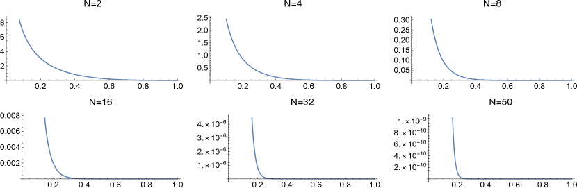
Figure 4: Plot of the difference $G(\eta)-\sum_{n=2}^{N}b_{n}\widetilde{G}_{n}(\eta)$, with $\widetilde{G}_{n}$ and $\widetilde{b}_{n}$ as defined by (5.2)-(5.3).

In order to address Point b) above, we make use of the Dirac Delta property of the function $H_{1}$ proved in Proposition 4.4, in order to reduce the integration domains to bounded sets. We have the following

Proposition 5.1.

The Key Inequalities 4.5 are satisfied if and only if there exists a constant $\kappa_{\tau}>0$ such that

$$\int_{x\prec\xi\prec(1,0)}{\bf 1}_{D(t,s,x)}(\xi)\sqrt{{\bf h}(z;s,\xi)}H_{1}(z;s,\xi)\sqrt{{\bf h}(s,\xi;{\bf 1}_{\mathbb{G}})}H_{1}(s,{\xi};{\bf 1}_{\mathbb{G}})d\xi \leq\kappa_{\tau}\,\sqrt{{\bf h}(z;{\bf 1}_{\mathbb{G}})}H_{1}(z,{\bf 1}_{\mathbb{G}}),\qquad$$ (5.6)

$$\int_{x\prec\xi\prec(1,0)}{\bf 1}_{D^{\prime}(t,s,x)}(\xi)\widetilde{g}\big{(}{{\bf h}(z;s,\xi)}\big{)}H_{1}(z;s,\xi)\widetilde{g}\big{(}{{\bf h}(s,\xi;{\bf 1}_{\mathbb{G}})}\big{)}H_{1}(s,{\xi};{\bf 1}_{\mathbb{G}})d\xi \leq\kappa_{\tau}\,\widetilde{g}\big{(}{{\bf h}(z;{\bf 1}_{\mathbb{G}})}\big{)}H_{1}(z,{\bf 1}_{\mathbb{G}}),\qquad$$ (5.7)

for any $s\in]t,0[$, and for any $z=(t,x)\in{\mathbb{R}}\times D$ such that $z\prec{\bf 1}_{\mathbb{G}}$ and $t>-\tau$, where $D(x),D^{\prime}(x)\subset D$ are the bounded domains

$$D(t,s,x) :=\Big{\{}\xi\in D:\Big{(}\sqrt{{\bf h}(z;s,\xi)}H_{1}(z;s,\xi)\Big{)}\wedge\Big{(}\sqrt{{\bf h}(s,\xi;{\bf 1}_{\mathbb{G}})}H_{1}(s,{\xi};{\bf 1}_{\mathbb{G}})\Big{)}>\sqrt{{\bf h}(z;{\bf 1}_{\mathbb{G}})}H_{1}(z,{\bf 1}_{\mathbb{G}})\Big{\}},\qquad$$ (5.8)

$$D^{\prime}(t,s,x) :=\Big{\{}\xi\in D:\Big{(}\widetilde{g}\big{(}{{\bf h}(z;s,\xi)}\big{)}H_{1}(z;s,\xi)\Big{)}\wedge\Big{(}\widetilde{g}\big{(}{{\bf h}(s,\xi;{\bf 1}_{\mathbb{G}})}\big{)}H_{1}(s,{\xi};{\bf 1}_{\mathbb{G}})\Big{)}>\widetilde{g}\big{(}{{\bf h}(z;{\bf 1}_{\mathbb{G}})}\big{)}H_{1}(z,{\bf 1}_{\mathbb{G}})\Big{\}}.$$ (5.9)

Proof.

By (5.8) we have

$$\int_{x\prec\xi\prec(1,0)}{\bf 1}_{D\setminus D(t,s,x)}(\xi)\sqrt{{\bf h}(z;s,\xi)}H_{1}(z;s,\xi)\sqrt{{\bf h}(s,\xi;{\bf 1}_{\mathbb{G}})}H_{1}(s,{\xi};{\bf 1}_{\mathbb{G}})\,d\xi$$ (5.10)

$$\leq\sqrt{{\bf h}(z;{\bf 1}_{\mathbb{G}})}H_{1}(z,{\bf 1}_{\mathbb{G}})\bigg{(}\int_{x\prec\xi}\sqrt{{\bf h}(z;s,\xi)}H_{1}(z;s,\xi)d\xi+\int_{\xi\prec(1,0)}\sqrt{{\bf h}(s,\xi;{\bf 1}_{\mathbb{G}})}\,{H_{1}(s,{\xi};{\bf 1}_{\mathbb{G}})}d\xi\bigg{)}.$$ (5.11)

Now, by Proposition 4.4 we obtain

$$\int_{x\prec\xi}\sqrt{{\bf h}(z;s,\xi)}H_{1}(z;s,\xi)\,d\xi=\int_{(1,0)\prec\xi}\sqrt{{\bf h}({\bf 1}_{\mathbb{G}};s-t,\xi)}H_{1}({\bf 1}_{\mathbb{G}};s-t,\xi)\,d\xi\longrightarrow 1,\qquad\text{as }s-t\to 0^{+},$$ (5.12)

and analogously

$$\int_{\xi\prec(1,0)}\sqrt{{\bf h}(s,\xi;{\bf 1}_{\mathbb{G}})}\,{H_{1}(s,{\xi};{\bf 1}_{\mathbb{G}})}\,d\xi=\int_{(1,0)\prec\xi}\sqrt{{\bf h}({\bf 1}_{\mathbb{G}};-s,\xi)}H_{1}({\bf 1}_{\mathbb{G}};-s,\xi)\,d\xi\longrightarrow 1,\qquad\text{as }s\to 0^{-}.$$ (5.13)

In particular, we have proved that the two integrals in (5.11) are bounded, for any $-\tau<t<s<0$ and $x\in D$, by a constant that only depends on $\tau$. Therefore, (5.6) is equivalent to (4.37). The proof that (5.7) is equivalent to (4.38) is identical. ∎

5.1 Numerical tests and results

In force of (5.4) and of Proposition 5.1 above, in order to prove the Key Inequalities 4.5 it is enough to check that

$$I_{1}(t,s,x):=\frac{\int_{]x_{2},0[\times]0,\bar{\xi}[}\sqrt{{\bf h}(z;s,\xi)}\widetilde{H}_{1}(z;s,\xi)\sqrt{{\bf h}(s,\xi;{\bf 1}_{\mathbb{G}})}\widetilde{H}_{1}(s,{\xi};{\bf 1}_{\mathbb{G}})d\xi}{\sqrt{{\bf h}(z;{\bf 1}_{\mathbb{G}})}H_{1}(z,{\bf 1}_{\mathbb{G}})} \leq\kappa_{\tau},$$ (5.14)

$$I_{2}(t,s,x):=\frac{\int_{]x_{2},0[\times]0,\bar{\bar{\xi}}[}\big{(}\sqrt{\bf h}+{\bf h}\big{)}(z;s,\xi)\widetilde{H}_{1}(z;s,\xi)\,\big{(}\sqrt{\bf h}+{\bf h}\big{)}(s,\xi;{\bf 1}_{\mathbb{G}})\widetilde{H}_{1}(s,{\xi};{\bf 1}_{\mathbb{G}})d\xi}{\big{(}\sqrt{\bf h}+{\bf h}\big{)}(z;{\bf 1}_{\mathbb{G}})H_{1}(z,{\bf 1}_{\mathbb{G}})} \leq\kappa_{\tau},$$ (5.15)

for any $z=(t,x)\in{\mathbb{R}}\times D$ such that $z\prec{\bf 1}_{\mathbb{G}}$ and $t>-\tau$, where $\widetilde{H}_{1}$ is defined as $H_{1}$ with $\Psi$ replaced by $\widetilde{\Psi}_{N}$ for a given $N>2$, and where $\bar{\xi},\bar{\bar{\xi}}>0$ are such that

$$]x_{2},0[\times]0,\bar{\xi}[\,\supset D(t,s,x)\,\cap\big{(}\,]x_{2},0[\times{\mathbb{R}}^{+}\big{)},\qquad]x_{2},0[\times]0,\bar{\bar{\xi}}[\,\supset D^{\prime}(t,s,x)\,\cap\big{(}\,]x_{2},0[\times{\mathbb{R}}^{+}\big{)}.$$ (5.16)

It is a direct computation to show that a possible choice for such $\bar{\xi},\bar{\bar{\xi}}$ is given by

$$\bar{\xi} =\max\bigg{\{}1,-\frac{x_{2}}{4}\Big{(}\Psi(t,x_{1},x_{2};{\bf 1}_{\mathbb{G}})-3\log\frac{t-s}{t}+\log 2\Big{)},\frac{x_{2}}{8}v^{*}\Big{(}\frac{8x_{1}}{x_{2}}e^{-2\big{(}\Psi(t,x_{1},x_{2};{\bf 1}_{\mathbb{G}})-3\log\frac{s}{t}+\log 2\big{)}+\frac{8x_{1}}{x_{2}}}\Big{)}\bigg{\}},$$ (5.17)

$$\bar{\bar{\xi}} =\max\bigg{\{}1,-\frac{x_{2}}{4}\Big{(}\Psi(t,x_{1},x_{2};{\bf 1}_{\mathbb{G}})-3\log\frac{t-s}{t}\Big{)},\frac{x_{2}}{8}v^{*}\Big{(}\frac{8x_{1}}{x_{2}}e^{-2\big{(}\Psi(t,x_{1},x_{2};{\bf 1}_{\mathbb{G}})-3\log\frac{s}{t}\big{)}+\frac{8x_{1}}{x_{2}}}\Big{)},$$ (5.19)

$$\qquad\qquad\frac{x_{2}}{4}v^{*}\Big{(}\frac{4x_{1}}{x_{2}}e^{-\big{(}\Psi(t,x_{1},x_{2};{\bf 1}_{\mathbb{G}})-3\log\frac{s}{t}\big{)}+\frac{4x_{1}}{x_{2}}}\Big{)}\bigg{\}},$$ (5.20)

with $v^{*}(\nu)$ being the lowest real solution to $\nu=ve^{v}$. The scope for turning the domains of integration into rectangles is facilitating the numerical integration.

We provide numerical evidence of the fact that (5.14)-(5.15) are satisfied for $\tau=1$, with $\kappa_{\tau}\approx 2.5$ and $N=50$. We test the inequalities for multiple choices of the parameters $s,t,x$, generated at random according to the following distributions:

$$t\sim\text{Unif}_{[-1,0]},\qquad s\sim\text{Unif}_{[t,0]},$$ (5.21)

and

$$x_{1}=\chi^{2},\qquad x_{2}=\frac{t\chi}{\eta},\qquad\text{with }(\chi,\eta)\sim\text{LogNorm}_{0,2}\otimes\text{LogNorm}_{0,2}.$$ (5.22)

The distribution above is justified by the representation (3.1), which can be written here as

$$\Psi(t,x;{\bf 1}_{\mathbb{G}})=\frac{4}{-t}\bigg{(}\eta\Big{(}\chi+\frac{1}{\chi}-2\Big{)}+G(\eta)\bigg{)},\qquad\eta={\bf h}(t,x;{\bf 1}_{\mathbb{G}})=\frac{t\sqrt{x_{1}}}{x_{2}},\ \chi=\sqrt{x_{1}},$$ (5.23)

and which shows that ${\Psi}$ reaches its minimum at $(\chi,\eta)=(1,1)$. We generated $2\times 10^{7}$ vectors $(s,t,x)$ and computed the integrals in the LHS of (5.14)-(5.15) using Monte Carlo integration. In Table 2 we report the maximum value of $I_{1}(t,s,x),I_{2}(t,s,x)$ and the corresponding $\arg\max$ obtained for the batch of variables. In Figure 5 we plot the $2\times 10^{7}$ samples of the pair $(\log\eta,\log\chi)$ generated at random with distribution $\mathcal{N}_{0,2}\otimes\mathcal{N}_{0,2}$, emphasizing the two argmax at which the maxima of $I_{1}$ and $I_{2}$ in Table 2 are attained.

The results do not present evidence of the fact that the functions $I_{1}$ and $I_{2}$ are unbounded. Note that, due to the chosen distributions for $(\eta,\chi)$ and $(t,s)$, the values of $I_{1}$ and $I_{2}$ were computed in a region that includes the extreme tails of the exponential kernel $e^{-\Psi(t,x;{\bf 1}_{\mathbb{G}})/2}$, and hence in a region where the denominators in (5.14)-(5.15) can be very small. For instance, for $t=-1/2,s=-1/4$ and $\chi=\xi=e^{8}$ one has $e^{-\Psi(t,x;{\bf 1}_{\mathbb{G}})/2}\approx 3.24\times 10^{-126}$.

The numerical integration was performed using Wolfram Mathematica built-in numerical integration routine NIntegrate with the method AdaptiveMonteCarlo. The Mathematica notebook used to generate the results reported above can be found in the supplementary material.

$n$	$t^{*}$	$s^{*}$	$x^{*}_{1}$	$x^{*}_{2}$	$\log\chi^{*}$	$\log\eta^{*}$	$I_{n}(t^{*},s^{*},x^{*})$
1	-0.81948	-0.54040	43.64581	-0.12497	1.88805	3.76863	1.74841
2	-0.78426	-0.67014	0.00002	-0.00605	-5.52146	-0.54472	2.48050

Table 2: The maxima $I_{n}(t^{*},s^{*},x^{*})=\max_{t,s,x}I_{n}(t,s,x)$ and relative argmax, with $t,s,x$ ranging over a batch counting $2\times 10^{7}$ samples generated at random in accordance with (5.21)-(5.22).

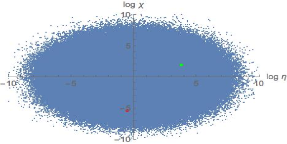
Figure 5: Blue dots: $2\times 10^{7}$ samples of the pairs $(\log\eta,\log\chi)$ generated at random with distribution $\mathcal{N}_{0,2}\otimes\mathcal{N}_{0,2}$. Green dot: pair $(\log\eta^{*},\log\chi^{*})$ at which the maximum $I_{1}$ in Table 2 is attained. Red dot: pair $(\log\eta^{*},\log\chi^{*})$ at which the maximum $I_{2}$ in Table 2 is attained.

Appendix A A topological lemma

Let $B=\big{\{}(x,y)\in{\mathbb{R}}^{2}\mid x^{2}+y^{2}<1\big{\}}$ denote the unit open ball of ${\mathbb{R}}^{2}$, and let $f:\overline{B}\to{\mathbb{R}}^{2}$ be a continuous map such that $f|_{\partial B}$ is a homeomorphism. In accordance with the Jordan-Schoenflies separation theorem, in the sequel $f(\partial B)^{*}$ will denote the “inside” of $f(\partial B)$, meaning the bounded set of ${\mathbb{R}}^{2}$, whose border is $f(\partial B)$, homeomorphic to an open ball. We will also denote by $f(\partial B)_{*}$ the “outside” of $f(\partial B)$, namely the complementary of $f(\partial B)\cup f(\partial B)^{*}$, which is homeomorphic to the complementary of a closed ball.

Lemma A.1.

Let $B$ be an open ball of ${\mathbb{R}}^{2}$, and let $f:\overline{B}\to{\mathbb{R}}^{2}$ be such that:

• $f$ is a local homeomorphism;

• $f|_{\partial B}$ is a homeomorphism.

Then $f|_{B}$ is a homeomorphism between $B$ and $f(\partial B)^{*}$.

Proof.

We first prove that

$$f(B)=f(\partial B)^{*}.$$ (A.1)

Assume that $f(\partial B)_{*}\cap f(\overline{B})\neq\emptyset$. Since $f(\overline{B})$ is a compact set, we also have $f(\partial B)_{*}\cap\big{(}f(\overline{B})\big{)}^{c}\neq\emptyset$. Therefore, being $f(\partial B)_{*}$ an open connected set, we have $f(\partial B)_{*}\cap\partial\left(f(\overline{B})\right)\neq\emptyset$. Let $y\in f(\partial B)_{*}\cap\partial\left(f(\overline{B})\right)$, again by compactness of $f(\overline{B})$ there exists $x\in\overline{B}$ such that $f(x)=y$. Note that $x\in B$, as $y\in f(\partial B)_{*}$. However, by (i), there exists a neighborhood $U$ of $x$ such that $f(U)$ is a neighborhood of $y$, which contradicts the fact that $y\in\partial\left(f(\overline{B})\right)$. We thus proved that $f(\overline{B})\subset\overline{f(\partial B)^{*}}$.

An analogous argument shows that $f(\overline{B})\supset\overline{f(\partial B)^{*}}$. Assume by contradiction that $f(\overline{B})\cap f(\partial B)_{*}\neq\emptyset$. Then $f(\partial B)^{*}\cap\partial\left(f(\overline{B})\right)\neq\emptyset$, and the conclusion follows. Thus,

$$f(\overline{B})=\overline{f(\partial B)^{*}}.$$ (A.2)

Moreover, if there were $x\in B$ such that $f(x)\in f(\partial B)$, then (i) would be violated because $f(\partial B)=\partial f(B)$. This proves (A.1).

We now note that the compact subsets in the subspace topologies on $B$ and $f(\partial B)^{*}$ are all the closed subsets of ${\mathbb{R}}^{2}$ contained in $B$ and $f(\partial B)^{*}$, respectively. Therefore, $f|_{B}:B\to f(\partial B)^{*}$ is a proper function.

Now, in order to conclude the proof it is enough to apply Hadamard-Caccioppoli Theorem, a particular instance of which states that a local homeomorphism between two open and simply connected sets of ${\mathbb{R}}^{n}$ is a global homeomorphism if and only if it is a proper function. ∎

Appendix B Proof of Lemma 4.1

Proof of Lemma 4.1.

First note that, by (2.19), it is enough to prove (4.17) for $w={\bf 1}_{\mathbb{G}}$. Now, we observe that it suffices to prove that

$$0=\inf_{\omega\in{\mathbb{R}}}\big{\{}\omega^{2}+\big{(}\omega x_{1}\partial_{x_{1}}+Y\big{)}\Psi(z,{\bf 1}_{\mathbb{G}})\big{\}},\qquad z=(t,x)\in{\mathbb{R}}\times D,\ z\prec{\bf 1}_{\mathbb{G}}.$$ (B.1)

Indeed, the function

$$\omega^{2}+\big{(}\omega x_{1}\partial_{x_{1}}+Y\big{)}\Psi(z,{\bf 1}_{\mathbb{G}})$$ (B.2)

has a global minimum at $\omega=-\frac{x_{1}}{2}\partial_{x_{1}}\Psi(z,{\bf 1}_{\mathbb{G}})$, which is

$$-\Big{(}\frac{x_{1}}{2}\partial_{x_{1}}\Psi(z,{\bf 1}_{\mathbb{G}})\Big{)}^{2}+Y\Psi(z,{\bf 1}_{\mathbb{G}}).$$ (B.3)

Consider now the following extended control problem. For any $z=(t,x)\in{\mathbb{R}}\times D$ with $z\prec{\bf 1}_{\mathbb{G}}$, and for any $x_{0}\in{\mathbb{R}}$, find

$$\bar{\Psi}(t,x_{0},x_{1},x_{2})=\min_{\omega}\gamma_{0}(T),$$ (B.4)

where the minimum is taken over all the controls $\omega\in L^{2}([t,T])$ for which (1.8) with $w={\bf 1}_{\mathbb{G}}$ are satisfied, and

$$\dot{\gamma}_{0}(s)=\omega^{2}(s),\quad t<s<T, \gamma_{0}(t)=x_{0}.$$ (B.5)

It is trivial to see that $\omega$ is optimal for this problem if and only if it is optimal for the problem (1.7)-(1.8). Also, we have

$$\bar{\Psi}(t,x_{0},x_{1},x_{2})={\Psi}(t,x_{1},x_{2};{\bf 1}_{\mathbb{G}})+x_{0}.$$ (B.6)

Therefore, (B.1) is equivalent to

$$0=\inf_{\omega\in{\mathbb{R}}}\big{\{}\big{(}\omega^{2}\partial_{x_{0}}\bar{\Psi}(t,x_{0},x)+\omega x_{1}\partial_{x_{1}}+Y\big{)}\bar{\Psi}(t,x_{0},x)\big{\}},\qquad z=(t,x)\in{\mathbb{R}}\times D,\ z\prec{\bf 1}_{\mathbb{G}},\quad x_{0}\in{\mathbb{R}}.$$ (B.7)

Eventually, the latter holds true by Theorem IV-4.1 in [10], which applies to the our problem as $\Psi(\cdot,{\bf 1}_{\mathbb{G}})$ is smooth on its domain and the optimal control $\omega$ is piecewise continuous. Theorem IV-4.1 in [10] also states (4.18), and this concludes the proof. ∎

References

- [1] D. G. Aronson, Bounds for the fundamental solution of a parabolic equation, Bulletin of the American Mathematical society, 73 (1967), pp. 890–896.
- [2] R. Azencott, Densité des diffusions en temps petit: développements asymptotiques. I, in Seminar on probability, XVIII, vol. 1059 of Lecture Notes in Math., Springer, Berlin, 1984, pp. 402–498.
- [3] G. Ben Arous, Développement asymptotique du noyau de la chaleur hypoelliptique hors du cut-locus, in Annales scientifiques de l’Ecole normale supérieure, vol. 21, 1988, pp. 307–331.
- [4] N. C. Caister, J. G. O’Hara, and K. S. Govinder, Solving the Asian option PDE using Lie symmetry methods, Int. J. Theor. Appl. Finance, 13 (2010), pp. 1265–1277.
- [5] G. Cibelli, S. Polidoro, and F. Rossi, Sharp estimates for Geman–Yor processes and applications to arithmetic average asian options, Journal de Mathématiques Pures et Appliquées, 129 (2019), pp. 87–130.
- [6] S. De Marco and P. K. Friz, Local volatility, conditioned diffusions, and varadhan’s formula, SIAM Journal on Financial Mathematics, 9 (2018), pp. 835–874.
- [7] J. N. Dewynne and W. T. Shaw, Differential equations and asymptotic solutions for arithmetic Asian options: ‘Black-Scholes formulae’ for Asian rate calls, European J. Appl. Math., 19 (2008), pp. 353–391.
- [8] D. Dufresne, Laguerre series for Asian and other options, Math. Finance, 10 (2000), pp. 407–428.
- [9] , Asian and Basket asymptotics, Research paper n.100, University of Montreal, (2002).
- [10] W. H. Fleming and R. W. Rishel, Deterministic and stochastic optimal control, vol. 1, Springer Science & Business Media, 2012.
- [11] P. Foschi, S. Pagliarani, and A. Pascucci, Approximations for asian options in local volatility models, Journal of Computational and Applied Mathematics, 237 (2013), pp. 442–459.
- [12] M. D. Francesco and A. Pascucci, On a class of degenerate parabolic equations of kolmogorov type, Applied Mathematics Research eXpress, 2005 (2005), pp. 77–116.
- [13] A. Friedman, Partial differential equations of parabolic type, Prentice-Hall Inc., Englewood Cliffs, N.J., 1964.
- [14] P. K. Friz, J. Gatheral, A. Gulisashvili, A. Jacquier, and J. Teichmann, Large deviations and asymptotic methods in finance, vol. 110, Springer, 2015.
- [15] M. Fu, D. Madan, and T. Wang, Pricing continuous time Asian options: a comparison of Monte Carlo and Laplace transform inversion methods, J. Comput. Finance, 2 (1998), pp. 49–74.
- [16] J. Gatheral, E. P. Hsu, P. Laurence, C. Ouyang, and T.-H. Wang, Asymptotics of implied volatility in local volatility models, Mathematical Finance: An International Journal of Mathematics, Statistics and Financial Economics, 22 (2012), pp. 591–620.
- [17] H. Geman and M. Yor, Quelques relations entre processus de Bessel, options asiatiques et fonctions confluentes hypergéométriques, C. R. Acad. Sci. Paris Sér. I Math., 314 (1992), pp. 471–474.
- [18] E. Gobet and M. Miri, Weak approximation of averaged diffusion processes, Stochastic Processes and their Applications, 124 (2014), pp. 475–504.
- [19] P. Guasoni and S. Robertson, Optimal importance sampling with explicit formulas in continuous time, Finance Stoch., 12 (2008), pp. 1–19.
- [20] J. E. Ingersoll, Theory of Financial Decision Making, Blackwell, Oxford, 1987.
- [21] R. Léandre, Majoration en temps petit de la densité d’une diffusion dégénérée, Probability theory and related fields, 74 (1987), pp. 289–294.
- [22] , Minoration en temps petit de la densité d’une diffusion dégénérée, Journal of Functional Analysis, 74 (1987), pp. 399–414.
- [23] V. Linetsky, The spectral decomposition of the option value, International Journal of Theoretical and Applied Finance, 7 (2004), pp. 337–384.
- [24] H. Matsumoto, M. Yor, et al., Exponential functionals of brownian motion, i: Probability laws at fixed time, Probability surveys, 2 (2005), pp. 312–347.
- [25] S. A. Molchanov, Diffusion processes and riemannian geometry, Russian Mathematical Surveys, 30 (1975), p. 1.
- [26] S. Pagliarani, A. Pascucci, and M. Pignotti, Intrinsic expansions for averaged diffusion processes, Stochastic Processes and their Applications, 127 (2017), pp. 2560–2585.
- [27] A. Pascucci, PDE and martingale methods in option pricing, Springer Science & Business Media, 2011.
- [28] D. Pirjol and L. Zhu, Short maturity asian options in local volatility models, SIAM Journal on Financial Mathematics, 7 (2016), pp. 947–992.
- [29] S. Polidoro, On a class of ultraparabolic operators of kolmogorov-fokker-planck type, Le Matematiche, 49 (1994), pp. 53–105.
-
[30]
W. T. Shaw, Pricing Asian options by contour integration,
including asymptotic methods for low volatility, Working paper,
http://www.mth.kcl.ac.uk/shaww/web_page/papers/Mathematicafin.htm, (2003). - [31] K. Shiraya and A. Takahashi, Pricing average options on commodities, forthcoming in Journal of Futures Markets, (2010).
- [32] K. Shiraya, A. Takahashi, and M. Toda, Pricing Barrier and Average Options Under Stochastic Volatility Environment, SSRN eLibrary, (2009).
- [33] S. R. Varadhan, Diffusion processes in a small time interval, Communications on Pure and Applied Mathematics, 20 (1967), pp. 659–685.
- [34] S. R. S. Varadhan, On the behavior of the fundamental solution of the heat equation with variable coefficients, Communications on Pure and Applied Mathematics, 20 (1967), pp. 431–455.
- [35] A. D. Ventsel’ and M. I. Freidlin, On small random perturbations of dynamical systems, Russian Mathematical Surveys, 25 (1970), pp. 1–55.
- [36] M. Yor, On some exponential functionals of Brownian motion, Adv. in Appl. Probab., 24 (1992), pp. 509–531.
- [37] K. Yosida, On the fundamental solution of the parabolic equation in a riemannian space, Osaka Mathematical Journal, 5 (1953), pp. 65–74.