Improving Patent Mining and Relevance Classification using Transformers

Abstract

Patent analysis and mining are time-consuming and costly processes for companies, but nevertheless essential if they are willing to remain competitive. To face the overload induced by numerous patents, the idea is to automatically filter them, bringing only few to read to experts. This paper reports a successful application of fine-tuning and retraining on pre-trained deep Natural Language Processing models on patent classification. The solution that we propose combines several state-of-the-art treatments to achieve our goal$\colon$decrease the workload while preserving recall and precision metrics.

Résumé

L’analyse et l’exploitation de brevets sont des processus longs et coûteux pour les entreprises, mais néanmoins indispensables si elles veulent rester compétitives. Pour faire face au nombre croissant de brevets à analyser, il est possible de procéder à un filtrage préliminaire automatique, afin de n’en sélectionner qu’un nombre limité, qui est par la suite analysé par des experts. Cet article présente les résultats obtenus sur un cas d’étude industriel. Des modèles d’apprentissage profond pré-entraînés, utilisés en Traitement Automatique de la Langue, ont été fine-tunés et ré-entraînés pour améliorer la classification de brevets. La solution que nous proposons combine plusieurs traitements de l’état de l’art pour atteindre notre objectif : diminuer la charge de travail des experts tout en préservant les mesures de rappel et de précision.

Mots-clés

Transformeurs, paramétrage, classification de brevets, traitement automatique de la langue naturelle, modèles de langage.

Keywords

Transformers, fine-tuning, patent classification, natural language processing, language models.

1 Introduction

Patents play one of the key roles in business intelligence. Mining state-of-the-art patents can help companies explore new or different ways of innovation to remain competitive. The conventional patent mining activity requires domain experts to manually evaluate all collected patents. A patent is considered relevant when matching the experts’ current interests regarding a given subject. When the number of patents increases exponentially, the manual annotation will be too time-consuming and too costly. Tools from Natural Language Processing (NLP) have been used to filter most likely irrelevant patents for years. Unfortunately, the classification rate is quite low in many real cases. In 2018, the biggest change in NLP was the introduction of language models based on Transformer [1]. BERT (Bidirectional Encoder Representations from Transformers) [1] obtained state-of-the-art results on eleven natural language processing tasks, including pushing the GLUE score to 80.5%. It is soon optimized by RoBERTa [2], which beat again the state-of-the-art results. These two have been once again improved in DeBERTa (Decoding-enhanced BERT with disentangled attention) [3]. GPT-2, another transformer model, can not only generate coherent paragraphs of text, but also achieve state-of-the-art performances on many language modeling benchmarks [4]. To better handle longer documents, Longformer was introduced in 2020 [5].

Many successful text classification applications have been reported, including classification of complex documents like patents [6, 7, 8, 9, 10, 11]. However, patent relevance classification remains a challenging problem. The “relevance” itself is context dependent. One will need to retrain or fine-tune the pre-trained models for specific applications.

The main aim of the project is to study the feasibility of building an automatic patent relevance evaluation tool to pre-classify collected patents and reduce the annotation load from experts for further evaluations. All patents classified as relevant by this tool, whether they are truly relevant or not, will then be manually appraised by experts. False positives are eventually rejected during the experts’ manual inspection. One critical aspect in patent relevance classification is: misclassifying as few relevant patents as possible is vital as each one holds a potential threat against the business, even though this leads to a slightly larger number of patents left to be manually labeled.

In this work, we report a successful application of fine-tuning on pre-trained deep NLP models on patent relevance classification, by benchmarking on state-of-the-art transformer models in order to find the most appropriate model(s) for this application.

2 Data and Models

2.1 Data

As aforementioned, the data that we consider are patents in English and, more precisely, their titles combined with the claims. Indeed, claims are the part containing key information about patents and highlight their essential elements [12]. Titles contain more general information, so they could also be used as features.

Figure 1: One claim from patent “Processing a 4D Seismic Signal Based on Noise Model” WO2019053484 [13]

Every year, thousands of patents for one topic only are being evaluated by Total SE. Amongst these patents, in general, only $10\%$ are considered relevant. As imbalanced classes are problematic for machine learning model training, we used an oversampling technique to solve this issue: by randomly duplicating relevant patents until their number is equal to the one of the other class.

2.1.1 Dataset topics

All the datasets in this work have been manually evaluated by experts. Two confidential topics have been studied here. The first topic (Topic A) has been followed by Total SE for more than 20 years, so relevant patents can be easily identified by the experts. This dataset is thus more homogeneous in terms of text diversity. It includes data from two successive years (named A1 and A2) as well as data from the first three quarters of a third year (named AT1, AT2 and AT3). The second topic (Topic B) has been tracked for only a few years and is a more heterogeneous group than topic A. It is composed of three sequential datasets (named B1, B2 and B3) over a period of one and a half years.

Topic A and topic B were only used to evaluate the transformers’ performances on different topics. Better results with topic A than with topic B are to be expected due to the nature of the datasets themselves and do not represent the point of interest of this study. Topic B has been studied to know whether newer topics could also benefit from the classification automation.

Any reference to a combination of several datasets of the same topic will be presented by concatenating the corresponding dataset names if no confusion may occur.

In the following table, size refers to the number of patents in each dataset.

Table 1: Approximate number of patents for each dataset.

Topic A	Size	Topic B	Size
A1	3,500	B1	6,500
A2	4,500	B2	1,500
AT1	1,500	B3	3,500
AT2	1,500
AT3	1,500

2.1.2 Training and testing strategies

The classification strategy implies to rely partly or entirely on history datasets for model training to predict the relevance of new datasets. For the datasets in Table 1, this led to the following train / test configurations$\colon$

Table 2: Training and testing dataset configurations.

Training datasets	Testing datasets
A1	A2
A12	AT123
AT12	AT3
A12T12	AT3
B1	B2
B1	B3
B12	B3

By default, for every model, the maximum sequence length is set to 512 tokens (except for Longformer where it has been set to 1,024 tokens), the batch size to 64, the learning rate to $2e-5$ with a linear scheduler with no warmup steps. Each model has been trained for 20 epochs.

Several pre-processings have been performed on these datasets, although not all of them have been used for each experiment. The datasets have firstly been re-sampled to avoid the imbalanced-class problem. For a given patent, its title and claims have been concatenated into a single string. The maximum sequence length is set to 512 tokens (about 450 words). However, when considering all the claims concatenated for one patent in our dataset, the median sequence length is closer to 1,000 tokens. In consequence, each patent’s group of claims longer than 512 tokens have been truncated into chunks up to a maximum of 512 tokens. Then, each chunk has been processed by the transformers as one separate patent with the same label as the other chunks. For a given patent, the mean and the median of the probabilities of each chunk, returned by the transformers, have been calculated, and the resulting probability has been assigned to that patent.

To indicate which strategy has been used for which experiment in Tables 4, 5, 6 and 3, the following naming rules have been used$\colon$

• Training and testing datasets are separated by an underscore.

• Suffix R$\colon$dataset has been re-sampled, its name is followed by a suffix R.

• Suffix T$\colon$titles have been concatenated to claims.

• Suffix EX$\colon$dataset has been extended – longer patents truncated into shorter chunks of 512 tokens.

If the training dataset has the title and/or the extended modifications, the test dataset will have the same tweaks.

For example, A1-TR-EX_A2-T-EX indicates that the training dataset A1 (first dataset of topic A) has the titles of the patents concatenated to the claims and has also been re-sampled and extended. The testing dataset, A2 (second dataset of topic A), has the title tweak as well as its claims transformed into chunks.

In order to maximize the classification rate and evaluate the relevance of different components of patents, many combinations have been tested$\colon$experiments with and without titles, re-sampling or extending changes.

2.2 Optimizations, Metric and Models

To better classify the patents, the whole patent should technically be taken into account. However, the maximal patent text lengths can go beyond the transformer models’ capacity. For most transformer models used in this work, the maximum token length is 512. GPT-2 supports 1,024 tokens while Longformer can accept up to 4,096 tokens.

Increasing the maximum token length requires more GPU VRAM, which amount is obviously limited. The first and simplest solution is to decrease the batch size. However, this reduction induces learning issues as smaller batches mean causing gradient to be more prone to noise. In heterogeneous datasets, patents are less similar from one batch to another, noise effect will be more important. Gradient accumulation has been applied in order to overcome this limitation. This technique allows accumulating the gradients over a given number of batches. After this, the model is being updated before resetting the gradient.

A possible solution is gradient checkpointing, that loads part of the activation network and recomputes the missing activation before operating the back-propagation, rather than loading the full graph. It trades off time for memory. However, as communications inter-GPUs take considerable time, this technique is less interesting for multi-GPU configurations.

Another way to limit the GPU VRAM consumption is to reduce the vocabulary size and token interaction file from tokenizers. The idea is to build the vocabulary only from the current dataset. For all the benchmarked models except DeBERTa, a unique list of all the tokens and interactions between those tokens encountered in each training and test set couples are kept. This helped to reduce by around 50% the vocabulary size and by 20% the interaction file for all the considered models for topic A, and by 60% and 25% for the same files for topic B. Reducing the vocabulary directly impacts the size of the input tensor fed to the models and thereby the amount of VRAM needed, while not increasing the execution time.

2.3 Introduction to specific metric

Patent relevance evaluation is not a simple text classification problem. Reducing the workload from experts’ manual annotations is also crucial. Common metrics only, like recall, precision or even $F1$ score, were not enough. A new metric is proposed here, taking into account the percentage of patents that will not be manually processed, and the proportion of relevant patents properly classified$\colon$

$$\mathcal{M}=(4*\mathrm{recall}+\mathrm{precision}+\mathrm{patents\ left})\ /\ 6$$ (1)

The patents left changes according to the number of irrelevant patents incorrectly classified as relevant, increasing when this number decreases, and vice-versa. It represents the amount of unnecessary workload that needs to be manually done. The coefficient $4$ multiplying the recall is to rank models according to their ability to answer the initial problem$\colon$high recall, low number of patents left to be manually handled. Its value has been set to follow the experts’ view on the models’ performances: by asking the experts which model would be preferred over which other according to their recall, precision and patents left scores.

As a reminder, in the business intelligence context, having a few more patents to be manually labeled (so more false positives) than missing truly relevant patents (false negatives) will always be preferred.

2.4 Models

The transformer models used in our study are state-of-the-art models$\colon$BERT, GPT2, RoBERTa, DeBERTa and Longformer.

Since BERT [1] is the first deeply bidirectional, unsupervised language representation (Transformer architecture), it is used here as a baseline model for all the different modifications in the experiments. GPT2 [4] is the first large scale generative model capable of generating realistic texts. Its token prediction ability can also be used for classification tasks when using specific tokens as class labels [14]. RoBERTa [2] is known to perform better in general compared to BERT, partly thanks to its rigorous training with ten times more data than BERT. DeBERTa was part of the combination of models giving the second-best results on GLUE and SuperGLUE benchmarks and, as both gather a wide range of general Natural Language Understanding tasks, implementing this model was promising.

Finally, as most of these models can only work with sequences of up to 512 tokens (1,024 for GPT2), and as our dataset has a median length of around 1,000 tokens for the considered patents, trying to implement Longformer with its maximum sequence length of 4,096 was obviously an interesting track. Moreover, Longformer is known to perform better than RoBERTa on tasks involving long documents.

All of the transformers have been adapted from Hugging Face [15].

3 Results

To evaluate the effects of each pre-processing on the datasets as well as the choices of the datasets themselves, 12 experiments have been performed. Furthermore, more combinations, presented hereinbelow, have been tested using BERT only.

3.1 Extensive BERT comparison

3.1.1 BERT results table introduction

To have a baseline for as many experiments as possible and to compare them to one another, running BERT in its base uncased version appeared as the simplest and most obvious solution. The experiment naming rules are those aforementioned in Section 2.1.2. The models’ name column has been replaced by the specific features, if any, as a unique model only has been used.

Table 3: Extensive BERT experiments. From left to right, the columns are$\colon$Specific feature, Recall, Precision, Percentage, Score $\mathcal{M}$, Score $F1$, Maximal Memory usage in GB and Total computing time in minutes.

Feature	R	P	%	$\mathcal{M}$	F1	GB	Time
A1_A2
	0.8330	0.6618	12.7	0.8252	0.7376	16	60
A1-R_A2
NVMem	0.9176	0.6131	15.1	0.8709	0.7351	18.8	82
	0.9039	0.5783	15.7	0.8546	0.7054	16	79
Mem	0.9039	0.5783	15.7	0.8546	0.7054	18.8	80
Batch-8	0.9497	0.4814	19.9	0.8629	0.6390	18.8	153
A1-R-EX_A2-EX
$\mathrm{BERT_{\bar{X}}}$	0.9542	0.4691	20.5	0.8629	0.6290	16.5	106
$\mathrm{BERT_{\tilde{X}}}$	0.9542	0.4691	20.5	0.8629	0.6290	16.5	106
A1-T_A2-T
	0.8673	0.6413	13.6	0.8436	0.7374	NA	58
A1-TR_A2-T
NV	0.9497	0.5912	16.2	0.8873	0.7287	17.6	79
	0.9474	0.5550	17.2	0.8780	0.6999	34	78
1-GPU	0.9451	0.5485	17.3	0.8751	0.6941	25.9	155
A1-TR-EX_A2-T-EX
$\mathrm{BERT_{\bar{X}}}$	0.8970	0.6164	14.6	0.8580	0.7307	16.6	110
$\mathrm{BERT_{\tilde{X}}}$	0.8970	0.6164	14.6	0.8580	0.7307	16.6	110
A12-TR_AT123-T
	0.9669	0.1535	44.3	0.7743	0.2650	NA	142
A12T12-TR_AT3-T
	0.8571	0.2426	18.2	0.7555	0.3782	3.2	173
AT12-TR_AT3-T
	0.8312	0.2092	20.5	0.7287	0.3342	NA	60
B1-TR_B2-T
	0.6739	0.6392	17.7	0.7118	0.6561	16.5	99
B1-R_B3
	0.7029	0.4462	23.1	0.6883	0.5459	16.5	105
B1-TR_B3-T
	0.7695	0.4368	25.8	0.7282	0.5572	16.5	108
B12-TR_B3-T
	0.7200	0.5362	19.7	0.7208	0.6146	21.8	128
B12-TR-EX_B3-T-EX
$\mathrm{BERT_{\bar{X}}}$	0.8895	0.3439	37.9	0.7756	0.4960	16.6	186
$\mathrm{BERT_{\tilde{X}}}$	0.8895	0.3421	38.1	0.7749	0.4942	16.6	186

Here, NV stands for No Vocabulary changes; Mem means that the memory has been more thoroughly monitored; Batch-8 is for the batch size, here only, the batch size has been decreased to 8 and the gradient accumulation step size has been increased to 8 instead of 1;$\mathrm{BERT_{\bar{X}}}$ and $\mathrm{BERT_{\tilde{X}}}$ respectively indicate that the mean or the median of probabilities, of all the chunks returned by BERT, for a given patent, is taken into account to classify it; 1-GPU means that the model is run on single-GPU mode, without any parallelization (instead of 4 for the other tests).

All results going forward will, by default, refer to score $\mathcal{M}$. For readability, each training-test combination has been numbered.

3.1.2 BERT results interpretation

To understand these tables, here is an example with the first line of experiment . The training dataset is the first one of topic A (A1), which has been re-sampled, the testing dataset is the second dataset of topic A (A2). Line $1$ has BERT’s vocabulary file not altered, and the memory has been thoroughly monitored during the whole run. The model’s recall score is $0.9176$ for a precision of $0.6131$. The percentage of patents left to be classified manually is $15.1\%$ of the total number of patents. This means that, if we decided to take into account the decision of the model for each patent, $15.1\%$ of all the patents would have been considered relevant by the model and manually classified, the rest would not have been further processed. The $\mathcal{M}$ score for this model is $0.8709$ and its $F1$ score is $0.7351$. The maximal amount of VRAM consumed is $18.8$GB and the total execution time is 82 minutes.

Experiment and line $2$ of experiment show that re-sampling the data yields better results (sequentially, Score $\mathcal{M}$=0.8252 against 0.8546, 2.94% better).

Experiments and show that concatenating the titles to the claims yields better results (sequentially, Score $\mathcal{M}$=0.8252 against 0.8436, 1.84% better).

Experiment and line $2$ of experiment show that combining re-sampling with concatenation of titles yield better results (sequentially 0.8252 against 0.8780, 5.28% better). Similar results can be observed with topic B.

Lines $1$ and $2$ of experiment show that using the original vocabulary from the tokenizer yields better results (sequentially 0.8873 against 0.8780, 0.93% better). The execution time is similar.

Lines $2$ and $3$ of experiment allow to check the influence of noise on the results as all randomness may not have been properly seeded. Here, the identical results confirmed that noise was not an issue.

Lines $2$ and $4$ of experiment show that decreasing the batch size to 8 while using a gradient accumulation with a step size of 8 yields better results (sequentially 0.8546 against 0.8629, 0.83% better).

Experiments , and show that $\mathrm{BERT_{\bar{X}}}$ and $\mathrm{BERT_{\tilde{X}}}$ yield almost identical results. However, experiments and , experiments and , and experiments and show that extending datasets does not systematically yield better results (respectively 8.3% better, 2.0% worse, 5.41% better with $\mathrm{BERT_{\bar{X}}}$ or 5.48% better with $\mathrm{BERT_{\tilde{X}}}$).

Lines $12$ and $3$ of experiment show that training and testing on only 1 GPU compared to 4 does not change significantly the results (0.29%), but the computing time has been drastically increased, here by two folds.

Experiments and show that using A12 along with AT12, for training, only improved the results by 2.7% but increased the total computing time by three folds (60 minutes when training on AT12, against 173). Depending on the retraining frequency, it might be more interesting to only use the most recent data as train dataset.

Experiments and show that adding B2 to B1 as training dataset and predicting on B3 did not yield way better results than using only B1 as training dataset (sequentially 0.7282 against 0.7208, so 0.74% better).

Similar results can be observed for topic B and its dataset (experiments through ). The rest of the results’ interpretation will be left to the reader.

The memory usage is the maximal amount used in the whole run. Values are just indicative and may be erroneous; models may work properly with lower amounts of memory as explained in Section 3.3.

3.1.3 BERT results conclusion

To conclude on this table, using the titles and re-sampling tweaks consistently led to better results (5.28% better for topic A). For two out of three cases, extending the datasets have yielded better results, even up to 5% for topic B. This may be an interesting track to follow for future studies. Moreover, as memory scarcity is an issue, decreasing the batch size, as well as limiting the vocabulary files, are promising trails that seem to not or only slightly decrease the performances. Besides, using the original vocabulary files yields better results and noise is not an issue for experiment reproducibility when seeds have been properly set.

3.2 Full results

3.2.1 Full results table introduction

Thanks to the powerful computing resources made available by Total SE, it has been possible to massively train different models on different dataset combinations with different strategies.

Hereunder, the detailed metrics for all the experiments are presented in Tables 4, 5 and 6. Only the best results, according to score $\mathcal{M}$ amongst the 20 epochs, have been kept and sorted in the result tables in decreasing order.

Table 4: Experiments 1 through 5. (Results ranked by descending metric $\mathcal{M}$ order).

MODEL	R	P	%	$\mathcal{M}$	F1
A1-R_A2
Mean	0.9359	0.5603	16.8	0.8717	0.7009
DeBERTa	0.9428	0.5372	17.7	0.8711	0.6844
Median	0.9359	0.5542	17.0	0.8703	0.6962
BERT	0.9039	0.5783	15.7	0.8546	0.7054
Longformer	0.9565	0.4274	22.5	0.8541	0.5908
GPT2	0.9291	0.4975	18.8	0.8532	0.6480
RoBERTa	0.8787	0.5818	15.2	0.8388	0.7001
A1-R-EX_A2-EX
$\mathrm{DeBERTa_{\bar{X}}}$	0.9519	0.4929	19.4	0.8670	0.6495
$\mathrm{DeBERTa_{\tilde{X}}}$	0.9519	0.4917	19.5	0.8667	0.6485
$\mathrm{BERT_{\bar{X}}}$	0.9542	0.4691	20.5	0.8629	0.6290
$\mathrm{BERT_{\tilde{X}}}$	0.9542	0.4691	20.5	0.8629	0.6290
Mean	0.8856	0.6627	13.5	0.8600	0.7581
Median	0.8833	0.6644	13.4	0.8588	0.7583
$\mathrm{GPT2_{\bar{X}}}$	0.9176	0.5434	17.0	0.8560	0.6826
$\mathrm{GPT2_{\tilde{X}}}$	0.9176	0.5434	17.0	0.8560	0.6826
$\mathrm{RoBERTa_{\bar{X}}}$	0.9314	0.4933	19.0	0.8538	0.6450
$\mathrm{RoBERTa_{\tilde{X}}}$	0.9314	0.4933	19.0	0.8538	0.6450
A1-TR_A2-T
Median	0.9451	0.5833	16.3	0.8826	0.7214
Mean	0.9405	0.5855	16.2	0.8801	0.7217
BERT	0.9474	0.5550	17.2	0.8780	0.6999
BERT-L	0.9245	0.6057	15.4	0.8739	0.7319
DeBERTa	0.9451	0.5329	17.8	0.8717	0.6815
RoBERTa-L	0.9588	0.4540	21.3	0.8622	0.6162
Longformer	0.9268	0.5407	17.3	0.8614	0.6830
GPT2-M	0.9062	0.5928	15.4	0.8592	0.7167
RoBERTa	0.9085	0.5712	16.0	0.8561	0.7014
GPT2	0.9176	0.5161	17.9	0.8500	0.6606
A1-TR-EX_A2-T-EX
$\mathrm{DeBERTa_{\bar{X}}}$	0.9588	0.5244	18.4	0.8787	0.6780
$\mathrm{DeBERTa_{\tilde{X}}}$	0.9588	0.5224	18.5	0.8782	0.6764
$\mathrm{RoBERTa_{\bar{X}}}$	0.9474	0.5049	18.9	0.8668	0.6587
$\mathrm{RoBERTa_{\tilde{X}}}$	0.9474	0.5049	18.9	0.8668	0.6587
Mean	0.8810	0.6912	12.8	0.8626	0.7746
Median	0.8787	0.6919	12.8	0.8612	0.7742
$\mathrm{BERT_{\bar{X}}}$	0.8970	0.6164	14.6	0.8580	0.7307
$\mathrm{BERT_{\tilde{X}}}$	0.8970	0.6164	14.6	0.8580	0.7307
$\mathrm{GPT2_{\bar{X}}}$	0.9039	0.5758	15.8	0.8541	0.7035
$\mathrm{GPT2_{\tilde{X}}}$	0.9039	0.5750	15.8	0.8539	0.7028
A12T12-TR_AT3-T
BERT-L	0.9221	0.1578	30.1	0.7654	0.2694
BERT	0.8571	0.2426	18.2	0.7555	0.3782
DeBERTa	0.8701	0.2030	22.1	0.7512	0.3292
Longformer	0.8571	0.2082	21.2	0.7448	0.3350
RoBERTa	0.8701	0.1791	25.0	0.7424	0.2971
Median	0.8312	0.2278	18.8	0.7346	0.3575
GPT2	0.8312	0.2169	19.7	0.7312	0.3441
Mean	0.8182	0.2308	18.3	0.7272	0.3600
RoBERTa-L	0.7792	0.2521	15.9	0.7083	0.3810
GPT2-M	0.6883	0.2611	13.6	0.6523	0.3786

In the first row of the table, the R stands for Recall, the P is Precision, the % is the percentage of patents classified as relevant, whether there gold label is relevant, and so left to be manually classified, the $\mathcal{M}$ refers to the proposed score, and the F1 is the $F1$ score. The next row has the training and testing datasets used and all the dataset modifications that have been applied. Then, each row represents the performances of a model on this training-test combination.

Mean is the mean of probabilities given by all the models for each patent; Median is their median. The suffixes $\mathord{\scalerel*{\Box}{gX}}_{\bar{X}}$ or $\mathord{\scalerel*{\Box}{gX}}_{\tilde{X}}$ of certain models follow the same nomenclature as in Section 3.1.1. Whenever the large version of a transformer was involved, a suffix L has been added to the model’s name. For GPT2, the M stands for the medium-sized version. Finally, the maximum sequence length used has been set to 512 for every model except for Longformer where it was 1,024 tokens.

3.2.2 Full results interpretation

Similarly to the previous Table 3, for each experiment, each line corresponds to one model with its values for recall, precision, patents left, score $\mathcal{M}$ and score $F1$.

In 10/12 experiments, DeBERTa is in the top two best models, followed by BERT/BERT large with 8/12. Longformer is in 3/9 top twos, when RoBERTa is in 2/12, and GPT2 reached it only once out of twelve experiments. The Mean and Median of all probabilities performed better than individual models respectively only three times and twice out of twelve. Note that these Mean and Median came from the best models obtained within the 20 epochs, so they may not be the best combinations that could exist in theory. However, testing all the possible cases is not possible. As an example, there are $2*(21^{8}-1)\approx 7.6e9$ possible combinations for experiment only.

In 8 experiments out of the 12 ones, Mean and Median are amongst the top three models. In 6/12 experiments, the Mean is better than the Median of probabilities. However, the mean difference in score $\mathcal{M}$ when the Mean is above the Median is only 0.0071, whereas this mean difference is 0.0238 when the Median is above the Mean. This shows that, although the Mean is above the Median in the same number of experiments, the Median should be the first choice as voting strategy.

To interpret part of the results in a clearer way, two experiments, designated by their numbers, will be compared to each other. To do so, the mean of score $\mathcal{M}$ of each individual model will be calculated for each couple of experiments compared. In other words, this mean will not include neither Mean nor Median. In the form of a listing, the first and the second experiments will be joined by an ”&” sign, followed by a coma and two scores, referring sequentially to the first and the second experiments, and joined by an ”&”. Finally, a colon ”$\colon$” will lead the interpretations.

Interpretation results$\colon$

• & , 0.8544 & 0.8599$\colon$extending the datasets yields better results (0.55%).

• & , 0.8544 & 0.8641$\colon$concatenating the titles to the claims yields better results (0.97%).

• & , 0.8641 & 0.8643$\colon$extending the datasets yields very slightly better results (0.02%).

• & , 0.7314 & 0.7051$\colon$although A1 and A2 are not part of the same year as AT123, using them alongside with AT12 for the training yields better results (2.63%).

• & , 0.7314 & 0.7711$\colon$training on A12 and testing on AT123 yields better results than training on A12T12 and testing on AT3 only (3.97%). Perhaps the patents in A12 are more similar to those in AT12 than in AT3. AT3 has also been published later than AT12 compared to A12.

• & , 0.7398 & 0.7020$\colon$training on B1 and testing on B2 yields better results than training on B1 and testing on B3 (3.78%). Once again, this may be due to the chronological distance being longer between B1 and B3 than between B1 and B2. Topic B being broader, patents considered to be relevant may vary faster with time than with other topics. This can mean that having recent datasets for training may be more critical than having more datasets but less updated.

• & , 0.7364 & 0.7020$\colon$training on B12 and testing on B3 yields better results than training on B1 and testing on B3 (3.44%). The possible interpretation is the same as the previous ones.

• & , 0.6717 & 0.7020$\colon$concatenating the titles to the claims yields better results (3.03%).

• & , 0.7364 & 0.7462$\colon$extending the datasets yields better results (0.98%). Having more data involved in the decision to classify patents, in one or the other class, may yield better results with topic B, as it is broader than topic A.

Table 5: Experiments 6 through 10. (Results ranked by descending metric $\mathcal{M}$ order).

MODEL	R	P	%	$\mathcal{M}$	F1
AT12-TR_AT3-T
BERT	0.8312	0.2092	20.5	0.7287	0.3342
Median	0.8052	0.2541	16.3	0.7255	0.3863
GPT2	0.7922	0.2699	15.1	0.7214	0.4026
Mean	0.7922	0.2629	15.5	0.7196	0.3948
Longformer	0.7662	0.2837	13.9	0.7081	0.4140
RoBERTa	0.7922	0.2089	19.5	0.7039	0.3306
DeBERTa	0.6494	0.4274	7.8	0.6634	0.5155
A12-TR_AT123-T
Mean	0.9307	0.2320	28.2	0.7897	0.3714
Median	0.9337	0.2240	29.3	0.7885	0.3613
BERT-L	0.9367	0.2160	30.5	0.7873	0.3510
Longformer	0.9578	0.1797	37.5	0.7839	0.3026
GPT2	0.9307	0.2071	31.6	0.7799	0.3388
BERT	0.9669	0.1535	44.3	0.7743	0.2650
RoBERTa-L	0.8735	0.2780	22.1	0.7687	0.4218
DeBERTa	0.8675	0.2815	21.7	0.7660	0.4251
RoBERTa	0.9518	0.1534	43.7	0.7652	0.2642
GPT2-M	0.8404	0.2640	22.4	0.7435	0.4017
B1-TR_B2-T
DeBERTa	0.7790	0.6324	20.7	0.7787	0.6981
Longformer	0.8732	0.3970	37.0	0.7778	0.5459
Mean	0.7862	0.5945	22.2	0.7749	0.6771
Median	0.8007	0.5525	24.4	0.7744	0.6538
RoBERTa	0.7572	0.4988	25.5	0.7333	0.6014
BERT	0.6739	0.6392	17.7	0.7118	0.6561
GPT2	0.7862	0.3196	41.4	0.6972	0.4545
B12-TR_B3-T
DeBERTa	0.8476	0.4555	27.3	0.7829	0.5925
Mean	0.8057	0.5146	22.9	0.7710	0.6281
Longformer	0.9352	0.2634	52.0	0.7702	0.4111
Median	0.8114	0.4936	24.1	0.7696	0.6138
RoBERTa	0.8876	0.3117	41.7	0.7625	0.4614
BERT-L	0.7886	0.4272	27.0	0.7378	0.5542
BERT	0.7200	0.5362	19.7	0.7208	0.6146
RoBERTa-L	0.6876	0.5841	17.2	0.7105	0.6317
GPT2-M	0.7562	0.3994	27.7	0.7096	0.5227
GPT2	0.7181	0.4425	23.8	0.6971	0.5476
B12-TR-EX_B3-T-EX
$\mathrm{BERT_{\bar{X}}}$	0.8895	0.3439	37.9	0.7756	0.4960
$\mathrm{BERT_{\tilde{X}}}$	0.8895	0.3421	38.1	0.7749	0.4942
$\mathrm{DeBERTa_{\bar{X}}}$	0.8343	0.4228	28.9	0.7655	0.5612
$\mathrm{DeBERTa_{\tilde{X}}}$	0.8343	0.4228	28.9	0.7655	0.5612
$\mathrm{GPT2_{\bar{X}}}$	0.7714	0.4540	24.9	0.7340	0.5716
$\mathrm{GPT2_{\tilde{X}}}$	0.7695	0.4524	24.9	0.7323	0.5698
$\mathrm{RoBERTa_{\bar{X}}}$	0.7105	0.5188	20.1	0.7107	0.5997
$\mathrm{RoBERTa_{\tilde{X}}}$	0.7105	0.5188	20.1	0.7107	0.5997
Median	0.6381	0.6879	13.6	0.6997	0.6621
Mean	0.6286	0.7006	13.1	0.6959	0.6627

In extended dataset experiments ( , and ), differences in $\mathcal{M}$ scores between the same models but attributing patents’ class with the median or mean of probabilities is minuscule (0.0283% on average).

In experiment , the best $F1$ score (with 0.5155) is ranked last according to score $\mathcal{M}$ as its recall is only of 0.6494, whereas the best model’s recall is 0.8312. Let us remind that, strategically speaking, it is important to miss as few relevant patents as possible, so a high recall will be preferred over a high precision at equal values. In experiment , the same situation occurs.

Scores with topic A are better than those of topic B. This may be due to the fact that patents in this topic are more general, and that topic B has only been tracked for a few years. These data are less refined, thus less representative, which makes the prediction task more challenging. Experiments and had similar configurations. Sequentially, without taking Mean nor Median into account, the maximal $\mathcal{M}$ scores are 0.8780 and 0.7829 (9.51%) and the mean of $\mathcal{M}$ scores are 0.8641 and 0.7364 (12.77%).

Table 6: Experiments 11 and 12. (Results ranked by descending metric $\mathcal{M}$ order).

MODEL	R	P	%	$\mathcal{M}$	F1
B1-R_B3
DeBERTa	0.8133	0.3509	33.9	0.7306	0.4902
Median	0.7219	0.4572	23.1	0.7032	0.5598
RoBERTa	0.7790	0.3264	35.0	0.7012	0.4601
Mean	0.7162	0.4619	22.7	0.7008	0.5616
BERT	0.7029	0.4462	23.1	0.6883	0.5459
Longformer	0.6381	0.4085	22.9	0.6376	0.4981
GPT2	0.5543	0.4763	17.0	0.6007	0.5123
B1-TR_B3-T
DeBERTa	0.8057	0.4862	24.3	0.7641	0.6065
Median	0.7543	0.5083	21.7	0.7364	0.6074
Mean	0.7505	0.5110	21.5	0.7346	0.6080
BERT	0.7695	0.4368	25.8	0.7282	0.5572
Longformer	0.7219	0.4019	26.3	0.6887	0.5163
RoBERTa	0.6838	0.4793	20.9	0.6843	0.5636
GPT2	0.6438	0.4214	22.4	0.6445	0.5094

In 3 out of 4 experiments, BERT large performed better than BERT base (0.895% better on average). In 2/4 experiments, GPT2 performed better than its medium equivalent (2.34%). The same occurred with RoBERTa large being better than its base version (1.91%).

Though Longformer is capable of taking much longer token sequences, it did not necessarily give better results than the other models. Longformer’s large version has also been tested for only one dataset combination by decreasing the maximal sequence length to 512. However, the results were worse than those of the base version, so experiments have not been pursued. Amongst the nine experiments where Longformer has been tested, 6/9 medians of the percentage of left patents of each individual model are lower than the individual score on the same metric that Longformer has. This model may be not decisive enough for our application.

3.2.3 Full results conclusion

Although topic A and B have very different $\mathcal{M}$ scores, the general trend remains the same$\colon$concatenating titles to claims, re-sampling the datasets and extending them yield better results. Moreover, datasets chronologically following each other give better results as topics are better depicted in datasets closer to the dataset to be tested. This is particularly true for broad topics as the ones that have not been monitored until recently. DeBERTa performs very consistently the best, while it was the exact contrary for GPT2. DeBERTa and BERT are more likely to be the first choices over other models when training time is limited. Even though neither Mean nor Median yielded the best results every time, it is still interesting to take them into account as, for most of the experiments, they were close to the top scores. Median is usually more secure to be kept.

3.3 GPU Memory usage and training time

The Figure 2 shows both training time and GPU VRAM used for each model.

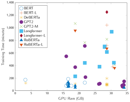
Figure 2: GPU memory usages and training times for different transformer models in all the experiments.

3.3.1 GPU Memory usage

Total SE’s HPC platform is equipped with multiple GPUs and CPUs. In this work, 4 Nvidia Tesla V100 (32GB VRAM) have been used. The peak GPU memory usage for all the tested models can be found in Figure 3. Note that GPU RAM usage reports might not be as accurate as expected. Several factors like GPU caching / RAM fragmentation / initialization etc. could prevent the program from returning the exact RAM usage information [16].

Using gradient accumulation allowed to run larger versions of the models, trading-off time for memory, with very limited performance influences.

For models with same data inputs and close parameter spaces, the maximal memory usage remains similar. These models have similar amounts of network parameters and input tensor dimensions, so the highest memory usages are at the same level. However, once the models have been initialized and are running in stable phase, much less VRAM is required. So, to correctly run these transformer models, one would need a GPU with at least 24GB or ideally 32GB of VRAM, otherwise, the model cannot even be initialized.

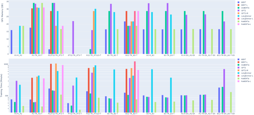
Figure 3: Detailed GPU memory usage and training time for different transformer models in all the experiments.

3.3.2 Training time

Memory requirements are surely an issue when it comes to training transformer models, but time can also be problematic. Here, the base models have been trained on 4 Nvidia Tesla V100 whereas larger models used only one V100 due to the gradient checkpointing technique. The preliminary benchmarking on gradient checkpointing showed, that there is no gain with multi-GPU training in the current environment. The GPU-GPU communication is much more time-consuming than the potential time-saving from the usage of multiple GPUs. Using a single V100 is faster in this case. The number of training epochs was 20 and the maximum sequence length was 512 tokens. In all tested cases, RoBERTa was the fastest, mostly followed by DeBERTa. If it was not the case, DeBERTa was usually only about 2 minutes slower than BERT or GPT2. As for GPT2, it depends on the datasets: it could perform as fast as the other models in some cases, but way slower for some other tests.

Larger versions of the models tend to need more time to run, due to the large parameter space and the gradient checkpointing application. Longformer, whether it was in its base form or not, took way longer than the other transformers. With a sequence length of 512 tokens on B12-TR_B3-T, base Longformer took 7 hours 20 minutes to complete the training, while large Longformer required 20 hours 50 minutes for the same task.

4 Conclusion

Our work aimed at determining a list of promising techniques and models to be used for business intelligence. Thanks to all the computing resources provided by Total SE, we were able to massively perform experiments with state-of-the-art transformer models and different parameter configurations.

The exhaustive BERT experiments allowed us to evaluate the effects of different features and modifications, both on the models themselves and on the training and test datasets.

Amongst the best techniques and models we have been able to test, concatenating titles to claims, re-sampling are essential. Extending the datasets can also be very interesting but may need more work to make it a reliable solution. The best model in terms of performances and resource consumption (both VRAM and time) is DeBERTa, closely followed by BERT. The intuition that a high-performing model on the GLUE and SuperGLUE tasks would also work efficiently for our use-case has paid off. Moreover, the BERT experiments showed, that reducing the batch size, along with using gradient accumulation, gave comparable results to those of models with an unchanged batch size, and achieved this while reducing the amount of VRAM required to run. Neither Longformer nor GPT2, both for their time consumption and performances, can be recommended for a similar task as the one in this study.

For topic A, the best combination of models (the Median) reached an $\mathcal{M}$ score of 0.8826 with a recall of 0.9451, a precision of 0.5833 and only 16.3% of the total patents left for manual classification by the experts. If originally, 2,000 patents were to be processed, this model would leave only about 300 patents for manual annotation, dividing by almost ten folds the workload of the experts. However, for topic B, results are slightly worse: the best combination of models (the Mean) reached an $\mathcal{M}$ score of 0.7710 with a recall of 0.8057, a precision of 0.5146 and 22.9% of the total patents left for manual labeling. Results regarding topic B are worse than those of topic A, most certainly because of the broadness of subjects represented in topic B’s patents.

5 Discussion

According to the extensive BERT experiments, it has been observed that the original vocabulary produced slightly better results than the customized vocabulary. Note that DeBERTa’s vocabulary files have not been modified. Its top performances may partly be explained by this difference. Since modifying the vocabulary means the transformers will be retrained, their weights are being modified, possibly leading to a slight impact on their performances.

BERT experiments also showed better results when used gradient accumulation and reducing the batch size. However, one can argue on the veracity of this result for every model-dataset combination. Gradient accumulation should not yield better performances than using a big enough batch size. Retraining transformer models with customized vocabularies may be usable for domain-specific tasks. However, as confirmed from the experiments, this training would require much more data to build a robust and better model.

Experiments and are distinguished by the non-use of A12 as training datasets in . Results are, as expected, better in . However, using 11,000 examples as the training dataset against only 3,000 for a mere increase of 2.63% in score $\mathcal{M}$ may not the most interesting time-performance trade-off. So, it is advised to use additional data only when the latter is close enough to the dataset to be predicted. In practice, a small margin, including more patents than the group considered as relevant by the transformers, is expected, and all of them will be manually analyzed. This is to minimize the risk of missing critical patents. The margin will depend on the transformers’ performances on a given topic and is to be determined accordingly.

We are aware that not having a low $\mathcal{M}$ score is relatively expected. However, reaching a high $\mathcal{M}$ score may be a very hard achievement (90+%), especially on broad or new topics as topic B. Although score $\mathcal{M}$, given in this study, is specific to the view of Total SE’s experts on the ratio of true positives to false positives, this metric may be utilized by other companies to similarly evaluate their models’ performances. For example, if missing a few more true positives but decreasing further down the workload is required, assigning a higher weight to the patents left score and a lower one to the recall can be considered.

The next steps would involve testing more models, larger versions, training / retraining our own transformer models, including more data from the patents like the descriptions or the abstracts, optimizing the dataset extension technique. A possible improvement might be the attribution of a weight to the probability of each chunk of claims according to their size in terms of tokens.

References

- [1] J. Devlin, M. Chang, K. Lee, and K. Toutanova, “BERT: pre-training of deep bidirectional transformers for language understanding,” CoRR, vol. abs/1810.04805, 2018.
- [2] Y. Liu, M. Ott, N. Goyal, J. Du, M. Joshi, D. Chen, O. Levy, M. Lewis, L. Zettlemoyer, and V. Stoyanov, “Roberta: A robustly optimized BERT pretraining approach,” CoRR, vol. abs/1907.11692, 2019.
- [3] P. He, X. Liu, J. Gao, and W. Chen, “Deberta: Decoding-enhanced bert with disentangled attention,” arXiv preprint arXiv:2006.03654, 2020.
- [4] A. Radford, J. Wu, R. Child, D. Luan, D. Amodei, and I. Sutskever, “Language models are unsupervised multitask learners,” OpenAI Blog, vol. 1, no. 8, 2019.
- [5] I. Beltagy, M. E. Peters, and A. Cohan, “Longformer: The long-document transformer,” arXiv preprint arXiv:2004.05150, 2020.
- [6] S. Choi, H. Lee, E. L. Park, and S. Choi, “A deep patent landscaping model using transformer and graph convolutional network,” CoRR, vol. abs/1903.05823, 2019, withdrawn.
- [7] S. Li, J. Hu, Y. Cui, and J. Hu, “Deeppatent: patent classification with convolutional neural networks and word embedding,” Scientometrics, vol. 117, no. 2, pp. 721–744, 2018.
- [8] A. H. Roudsari, J. Afshar, C. C. Lee, and W. Lee, “Multi-label patent classification using attention-aware deep learning model,” in 2020 IEEE International Conference on Big Data and Smart Computing (BigComp). IEEE, Feb. 2020.
- [9] A. C. Marco, J. D. Sarnoff, and C. A. deGrazia, “Patent claims and patent scope,” Research Policy, vol. 48, no. 9, p. 103790, Nov. 2019.
- [10] J. Hu, S. Li, Y. Yao, L. Yu, G. Yang, and J. Hu, “Patent keyword extraction algorithm based on distributed representation for patent classification,” Entropy, vol. 20, no. 2, p. 104, Feb. 2018.
- [11] J.-S. Lee and J. Hsiang, “Patent classification by fine-tuning bert language model,” World Patent Information, vol. 61, p. 101965, 2020.
- [12] L. Zhang, L. Li, and T. Li, “Patent mining: A survey,” SIGKDD Explor. Newsl., vol. 16, no. 2, p. 1–19, May 2015.
- [13] C. Hubans and N. Shchukina, “Processing a 4d seismic signal based on noise model,” FR Patent WO2 019 053 484, 9 18, 2017.
- [14] B. Xu, C. Gil-Jardiné, F. Thiessard, E. Tellier, M. Avalos, and E. Lagarde, “Pre-Training a neural language model improves the sample efficiency of an emergency room classification model,” in The 33rd Florida Artificial Intelligence Research Society Conference, 2020.
- [15] T. Wolf, L. Debut, V. Sanh, J. Chaumond, C. Delangue, A. Moi, P. Cistac, T. Rault, R. Louf, M. Funtowicz, J. Davison, S. Shleifer, P. von Platen, C. Ma, Y. Jernite, J. Plu, C. Xu, T. Le Scao, S. Gugger, M. Drame, Q. Lhoest, and A. Rush, “Transformers: State-of-the-art natural language processing,” in Proceedings of the 2020 Conference on Empirical Methods in Natural Language Processing: System Demonstrations. Online: Association for Computational Linguistics, Oct. 2020, pp. 38–45.
- [16] fastai, “Working with gpu,” in fastai Documentation, Mar 13, 2021.