Graph Inference Representation: Learning Graph Positional Embeddings with Anchor Path Encoding

Abstract

Learning node representations that incorporate information from graph structure benefits wide range of tasks on graph. The majority of existing graph neural networks (GNNs) have limited power in capturing position information for a given node. The idea of positioning nodes with selected anchors has been exploited, yet mainly relying on explicit labeling of distance information. Here we propose Graph Inference Representation (GIR), an anchor based GNN model encoding path information related to pre-selected anchors for each node. Abilities to get position-aware embeddings are theoretically and experimentally investigated on GIR and its core variants. Further, the complementarity between GIRs and typical GNNs is demonstrated. We show that GIRs get outperformed results in position-aware scenarios, and performances on typical GNNs could be improved by fusing GIR embeddings.

1 Introduction

Graph, as an important data structure, is a powerful tool to represent ubiquitous relationships in the real world. Learning vector representations for graph data, benefits many downstream tasks on graph such as node classification [9] and link prediction [25]. Many graph representation learning methods have been proposed recently, among those, Graph Neural Networks (GNNs), inheriting the merits of neural networks, have shown superior performance and become a much popular choice.

Existing GNN models mainly follow the message passing neural network (MPNN) [4] pattern, which stacks MPNN layers that aggregate information from neighborhoods and then update representations for each node. Typical MPNNs have been shown to lack of ability to capture the position information within graph [22], without distinguishable node/edge attributes, nodes in different part of the graph with topologically equivalent neighborhood structures will be embedded into the same representation by typical MPNNs alone [22, 11], Figure 1 gives an example.

Researchers have developed methods to alleviate this issue. Some earlier works adopt one-hot encodings as extended node attributes [9]. More recent anchor based methods [22, 12] select anchor nodes as positioning base, use position information related to anchors to break the structural symmetry, Figure 1 shows some cases of this strategy. Existing anchor based methods mainly directly pass message from anchors to each node, for modeling positional relationship, distance information from anchors are explicitly assigned as node attributes. However, this strategy ignores the graph structure information to some extent, and the performance is strongly relying on the quality of the explicitly assigned information.

In this paper, we propose an anchor based GNN model, termed Graph Inference Representation (GIR), aiming at encoding path information related to pre-selected anchor nodes. GIRs first select fixed anchor nodes heuristically, messages are propagated from anchors along paths to each node, and outputs of the k-th layer encode k-order representations related to anchors.

Our contributions are summarized as follows:

1. We propose the Graph Inference Representation (GIR) model that follows the anchor based graph neural network (A-GNN) pattern. GIRs perform anchor path encoding by propagating message along paths from anchors.

2. We theoretically investigate the application of GIRs in position-aware scenarios, several variants are proposed to get more accurate positioning. We evaluate the performance of GIR and those variants for tasks in position-aware datasets, experimental results show that our position-aware GIRs archive generally higher performance.

3. We exploit the complementarity between GIRs and MPNNs, and adopt multi-modal fusion techniques to get benefit from this merit, experimental results demonstrate the improvement.

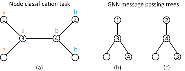
Figure 1: Node classification on the structral symmetric cases. (a) Example unattributed graph that assign different labels (a and b) on nodes with structral symmetry. (b&c) MPNNs message passing tree of node $v_{1}$ and $v_{2}$, message propagate from leaves to the root. Distinguishability: For $v_{1}$ and $v_{2}$, (1)No anchors: indistinguishable due to identity sub-structure; (2)$v_{3}$ or $v_{4}$ as anchor: distinguishable by different position from the anchor node; (3)$v_{3}$ and $v_{4}$ as anchors: distinguishable if the order of $v_{3}$ and $v_{4}$ is aware, indistinguishable otherwise.

2 Related works

2.1 Graph Neural Networks and anchor based methods

A large amount of existing GNN models follow the MPNN pattern, with different neighborhood aggregation and node representation update functions. Graph Convolution Networks (GCN) [9] uses normalized mean aggregator; GraphSAGE [5] concatenates node’s representation and neighborhood information from mean/max/LSTM aggregator; Graph Attention Network (GAT) [18] introduces attention mechanism in the neighborhood aggregation step. Our GIR model uses the same aggregate and update propagation strategy as MPNNs, but with different message propagation paths.

Anchor based GNN (A-GNN) methods follow the intuition that some nodes play more important role in the graph. Existing A-GNN models mainly follow the two stage pattern: select anchor nodes first, and then encode the information related to anchors. Position-aware GNN (PGNN) [22] proposes to position nodes with selected anchor nodes. PGNNs select anchor node sets randomly before running every forward of the model to get a low distortion embedding with global position information, an order-aware output layer was proposed to generate position-aware embedding for each node from anchor node sets, the output layer generates a vector representation whose elements are computed by messages directly received from corresponding anchor node set. The random anchor selecting strategy of PGNNs leads to unstable limitation, some more recent work use fixed anchor nodes instead to overcome this issue. AGNN [12] pre-selects fixed anchors by minimum point cover nodes algorithm; GraphReach [15] follows the fix anchor setting, and captures global positions of nodes by random walk reachability estimations instead of the shortest path distance. Other than selecting anchors as positioning base, Graph Inference Learning (GIL) [21] views nodes in the training set as anchors, and boosts the semi-supervised node classification performance by learning the inference of node labels on graph topology. Our GIR model is designed for position-aware scenarios, and differs existing A-GNN models in the anchor information encoding strategy.

2.2 Multi-modal Fusion

Multi-modal fusion aims at integrating information from multiple modalities, which could be categorized as early and late approaches [3]. Early fusion, or feature fusion, makes decision on fused representation. Representative methods of early fusion include gated fusion [2], and bilinear model [24, 13]. Late fusion, or decision fusion, make decisions on each uni-modal and fuses them for the final decision. Mixture of Experts (MoE) [7] is a representative late fusion model, which incorporate a gating network to decide which expert to use for each input. Widely used gating strategy in multi-modal fusion may face with fusion weights inconsistency issue, [17] suggest using uni-modal outputs loss to regularize fusion weights. We adapt MoE model for graph data, and use it to exploit the complementarity between GIRs nad MPNNs, strategies for fusion inconsistency issue are adopted.

3 Preliminaries

Table 1: Notations

Notation	Description
$\mathcal{G}$	the input graph
$\mathcal{V,E}$	the node/edge set of $\mathcal{G}$
$v_{i}$	the i-th node in $\mathcal{G}$
$\mathcal{X}$	the node attributes of $\mathcal{G}$
$\mathcal{Z}$	the node representations of $\mathcal{G}$
$x_{i},z_{i}$	the attribute/representation of $v_{i}$
$\mathcal{N}(v)$	in-neighborhoods of node v in $\mathcal{G}$
$\mathcal{A}$	the anchor node set
$\mathnormal{A}$	set of subsets of $\mathcal{A}$
$n$	the number of nodes

3.1 Notations and problem definition

A graph can be represented as $\mathcal{G=(V,{E})}$, where $\mathcal{V}=\{v_{1},\cdots,v_{n}\}$ is the node set and $\mathcal{E}=\{\langle v_{i},v_{j}\rangle|v_{i},v_{j}\in\mathcal{V}\}$ is the edge set. Nodes are augmented with the feature set $\mathcal{X}=\{x_{1},\cdots x_{n}\}$, which is either input attributes or placeholders if no attributes available. In-neighborhoods of node $v$ are represented as $\mathcal{N}(v)$. Notations are summarized in Table 1

The GIR model is designed for node representation learning task, which takes graph $\mathcal{G=(V,E)}$ with node attributes $\mathcal{X}$ as input, and embed nodes into d-dimensional vectors, represented as $\mathcal{Z}=\{z_{1},\cdots z_{n}\},z_{i}\in\mathbb{R}^{d}$. The node representations are normally used in downstream tasks like node classification and link prediction.

3.2 Position-aware embeddings

One goal of the anchor based GNN model is to utilize anchors as bases to encode position aware information for each node. To capture this intuition, PGNNs [22] view embeddings as position-aware if shortest path distance between node pairs could be reconstructed from their embeddings (Definition 1).

Definition 1 (Position-aware Embeddings).

A node embedding $z_{i}=f_{p}(v_{i}),\forall v_{i}\in\mathcal{(}V)$ is position-aware if there exists a function $g(\cdot,\cdot)$ such that $d_{sp}(v_{i},v_{j})=g(z_{i},z_{j})$, where $d_{sp}(\cdot,\cdot)$ is the shortest path distance in $\mathcal{G}$.

For models with fixed anchors, the shortest path distance between two nodes may not path through anchors, thus hard to satisfy definition 1. To capture the characteristic of position modeling for fixed anchors models, here we define position-aware embeddings related to anchors (Definition 2). Considering the differences of anchor utilization strategies (Figure 1, b&c), our definition of position aware embeddings is made on a set of anchor node sets.

Definition 2 ($\mathnormal{A}$-position-aware Embeddings).

For $\mathnormal{A}\subset\mathcal{P(A)},\bigcup_{\mathnormal{A}}=\mathcal{A}$, where $\mathcal{P(A)}$ is the power set of node set $\mathcal{A}$, a node embedding $z_{i}=f_{p}(v_{i}),\forall v_{i}\in\mathcal{V}$ is $\mathnormal{A}$-position-aware if there exists functions $\{g_{\mathcal{A}^{\prime}}(\cdot)|\forall\mathcal{A}^{\prime}\in\mathnormal{A}\}$ such that $g_{a}(z_{i})=d_{sp}(v_{i},\mathcal{A}^{\prime})$ where $d_{sp}(v,\mathcal{A}^{\prime})$ is the shortest path distance between node v and node set $\mathcal{A}^{\prime}$. If all elements in $\mathnormal{A}$ are singleton, brakets of sets inner $\mathnormal{A}$ could be omitted.

4 Proposed methods

In this section, we illustrate the key aspects of GIR model. We first describe the main framework and key components of GIRs. Next we propose position-aware variants which enable more accurate positioning, design choices and theoretical analysis are discussed. Then, we describe the fusion strategy for exploiting the complementarity between GIRs and MPNNs.

4.1 The framework of GIRs

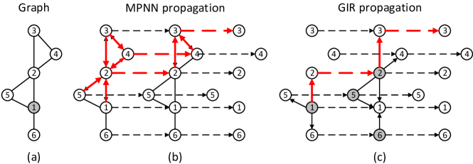
Figure 2: Message propagation paths for MPNNs and GIRs. (a) Example graph $\mathcal{G}$, nodes in grey are selected as anchors for anchor based GNNs. (b&c) Message propagation paths on $\mathcal{G}$ for a two layer MPNN (b) and GIR (c); solid line represents $Aggregate$; dot line represents $Update$. Grey nodes in (c) represent message passing sources on corresponding layer. Bold arrows in red highlight the propagation paths to node $v_{3}$.

We propose Graph Inference Representation (GIR) model that learns to integrate information from paths related to anchors for each node. GIRs propagate information on k-order ego graph of anchors, which contains k-step paths starting from anchors. For computing node representations, GIRs apply MPNN layers step by step, propagate information from anchors to each node (Figure 2, c). Algorithm 1 summarizes the framework of GIRs, where remains some key components to be elaborated: anchor selection and message passing functions.

Anchor Selection

The intuition behind anchor based GNNs is that some nodes perform more important role in the graph for the specific task [12, 21]. For getting position-aware embeddings on general tasks with no nodes performing special role, we heuristically prefer anchors to have high centrality and effective coverage through k-step message passing. We adopt GA-MPCA algorithm used in AGNN [12] as default choice, which select anchors according to degree centrality, giving attention to coverage and information interaction intensity.

Message Propagation

GIRs use adapted MPNN layers for message propagation, which contains neighborhood message passing and node state update steps (Algorithm 1, line 6-7). The key difference between GIRs and MPNNs is that the k-th layer of a GIR model only applies on edges on k-step away from anchors instead of whole edges. From the view of a specific node, a k-layer MPNN model learns to encode its k-hop ego network information, while a k-layer GIR model encode k-order representations related to anchors (Figure 2).

Note that it is an expected manner for GIRs that if the node $v$ has no propagation edge on the layer $l$, its message in $l$ would be a zero vector, and the MPNN layer $l$ would be degraded to a single layer perceptron for $v$. Thus, GIRs can be viewed as a hybrid of MPNNs and MLPs. From the view of GIRs, MPNNs use all nodes as anchors, while MLPs use none.

We take the full-batch GraphSAGE layer [5] as default message propagation function choice, concretely, we use mean function as aggregator and single layer perceptron as update function.

Input: Graph $\mathcal{G=(V,E)}$;number of layer $L$;node input attributes $\{x_{v},\forall v\in\mathcal{V}\}$;anchor selection function $SelectAnchor$;neighborhood aggregator functions $Aggregate_{l}$;node update functions $Update_{l}$

Output: A-position-aware embedding $\{z_{v},\forall v\in\mathcal{V}\}$

1 $\mathcal{A}\leftarrow SelectAnchor(\mathcal{G})$;

$\mathcal{SRC}\leftarrow\mathcal{A}$ ;

  /* $SRC$ keeps the propagation source nodes */

$h^{0}_{v}\leftarrow x_{v},\forall v\in\mathcal{V}$ ;

  /* $h_{l}^{v}$ represents hidden state of node $v$ on layer $l$ */

2 for $l\leftarrow 1$ to $L$ do

3       for $v\in\mathcal{V}$ do

             $m_{v}\leftarrow Aggregate_{l}(\{h_{u}^{l-1},\forall u\in\mathcal{N}(v)\cap\mathcal{SRC}\})$ ;

              /* message on node $v$ */

4             $h_{v}^{l}\leftarrow Update_{l}(h_{v}^{l-1},m_{v})$;

5            

6       end for

7      $\mathcal{SRC}\leftarrow Sussessors(\mathcal{G},\mathcal{SRC})$;

8      

9 end for

10$z_{v}\leftarrow h_{v}^{L}$;

Algorithm 1 The framework of GIRs

4.2 Position-aware GIRs

In this part, we show to what extent the GIR model helps break structural symmetry, variants are proposed to get more powerful position aware ability in the context of definition 2.

4.2.1 GIRs

Considering an unattributed graph $\mathcal{G}$, for MPNNs, nodes with equivalent sub-structure will be indistinguishable. GIRs truncate the message propagation path by anchors, thus break sub-structural equivalence for nodes at different positions (Figure 1).

For commonly used order agnostic neighborhood aggregator (e.g. mean), without properly identification, every anchor node plays the same role, thus position of each node related to a specific anchor node can not be discriminated. We show that the vanilla GIRs provide positioning ability with the overall anchor node set. We use commonly used mean function as aggregator, appropriate designed MLPs as update functions to meet the assumption of universal approximation theorem [6], GIR propagation depth is assumed enough to cover all reachable nodes from anchors.

Theorem 1.

GIRs are {$\mathcal{A}$}-position-aware.

Theorem 1 states that for any graph there exists a parameter setting of GIRs to get {$\mathcal{A}$}-position-aware embeddings, while in practice, the learned model is dedicated to the downstream task. The full proof of Theorem 1 is in the Appendix, the proof construct a well-defined message propagate function (depicted in Figure 3, a), the existence of parameter setting is guaranteed by the universal approximation theorem.

4.2.2 GIR-MIX: multiple anchor set

As GIRs are {$\mathcal{A}$}-position-aware, if multiple anchor sets are further selected, and applying GIRs on each, more fine-grained positioning ability could be got. We summarize the position-aware ability of this GIR-MIX model as follows:

Corollary 1.

GIR-MIXs with anchor sets $\mathnormal{A}=\{\mathcal{A}_{1},\cdots,\mathcal{A}_{n}\}$ are $\mathnormal{A}$-position-aware.

Instead of concatenating outputs only on the last layer, we further extend the representation power by concatenate outputs in every layer, and send the fused hidden layer outputs to the next layer. The GIR-MIX model could apply on transductive setting only, for the order of anchor sets is aware.

4.2.3 GIR-A: GIRs with anchor labeling

Inspired by the one-hot labeling trick used in previous works, and considering the concept of anchors in anchor based GNNs, we extend node attributes by one-hot labeling for anchors, and zero vector for other nodes. It gives identification for anchors, thus makes more accurate position. Also, compared with global node one-hot labeling, it has much lower input dimension. As the anchor identification cannot be generalized, the GIR-A model could apply on transductive setting only.

We show that with the anchor identification, position related to a specific anchor could be represented. Similar with the GIRs case, we adopt mean aggregator, update function model and propagation depth are properly chosen.

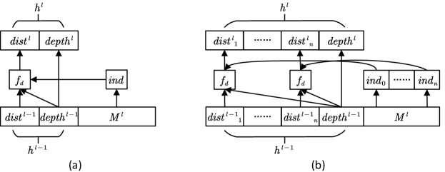
Figure 3: A construction of message passing function retaining distance information for GIRs (a) and GIR-As (b)

Theorem 2.

GIR-As are $\mathcal{A}$-position-aware.

The full proof of Theorem 2 is in the Appendix, the construction of the update function for the proof is depicted in Figure 3, b.

4.3 GCN-GIR: multi view fusion

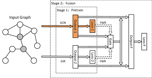
Figure 4: Overall architecture of GCN-GIRs. Stage 1 (pretrain stage) pretrain each expert alone, Stage 2 (fusion stage) freeze pretrained experts and train fusion part of the model.

One possible shortcoming for GIRs is that they work on only k-ego graph from anchors, with other edges unrelated, which may lose some useful information. The influence of this issue depends largely on the choice of anchors.

In fact, considering that a GIR model encode information related to anchors for each node, it utilizes graph structure information in a biased interest, thus learns another view of graph information compared with MPNNs. Thus, it is a natural idea to exploit the possibility of fusing MPNNs and GIRs in a complementary manner. As an example model, we take GCN and vanilla GIR as bases, and terms it GCN-GIR. Overall architecture of GCN-GIR is shown in Figure 4.

We adopt decision fusion strategy, and follow the idea of Mixture of Experts (MoE) [7]. Some details would be focused due to the non-independent nature of the graph data. First, outputs of all experts are used instead of inputs to compute fusion gate. This break the intuition of MoEs that dispatch independent data item to appropriate classifier, but more reasonable in this case as inputs of individual node may not enough to make decision. However, this strategy makes the gate for each expert relevant to other experts, which may make training process unstable. To alleviate this issue, we adopt a two-stage training strategy, which first pretrain each expert alone, then freeze all experts, train only the fusion part of the model.

We further adopt fusion weight regularization (FWR) [17], which follow the idea that experts with lower loss matters more, thus improve the consistency of the fusion gate and expert importances.

5 Experiments

In this section, we demonstrate performance of GIRs by two series of experiments. We first take experiments on datasets from position-aware GNN model literature to evaluate the performance of GIRs on position aware scenario. To evaluate the representation bias of GIRs to MPNNs, and the effect of multi view information fusion idea, we take experiments on much larger scale node classification task from Open Graph Benchmark [20]. All datasets are anonymous.

5.1 Position-aware GIRs

Datasets

We take datasets from previous position-aware GNN literature [22, 11], with MIT license. Those datasets with too few scales or unfit for transductive setting are filtered out, for unattributed graphs, we set node input attributes to ones as placeholders. Details of the dataset are listed in Table 2

Table 2: Details of position-aware datasets.

Dataset	$|\mathcal{V}|$	$|\mathcal{E}|$	Description
Email	920	14402	a real-world communication graph from SNAP [10]
Europe	399	5995	a flight network between airports in Europe [1]
USA	1190	13599	a flight network between airports in USA [1]
C.ele	297	2148	a neural network of C.elegans [8]
NS	1461	2742	a collaboration network between network science scientists [14]
PB	1222	16714	a political post web-page reference network [1]

Baselines

We choose baselines from MPNNs and anchor based methods literature. We choose representative method GCN [9] as MPNN baseline, for a fair comparison, random walk laplacian is used instead of symmetric normalized laplacian used in the origin paper. PGNN and AGNN are chosen as anchor based baselines, PGNN learns global position by random select anchors before each run, while AGNN is a representative GNN method using fixed anchor. Two variants of PGNN and AGNN are considered: using truncated 2-hop shortest path distance (PGNN-E/AGNN-F) and using exact shortest path distance (PGNN-E/AGNN-E).

We take experiments for vanilla GIR and several variants: (1) GIR with multiple anchor sets (GIR-MIX); (2) GIR with anchor labeling (GIR-A); (3) GIR with node one-hot labeling (GIR-O). As a general trick, anchor labeling and node one-hot labeling are also applied in MPNN baselines (GCN-A/GCN-O).

Experimental setup

Our experiments are taken on transductive setting. For node pair level tasks, 80% pairs are used for training, and 10% each as validation and test sets. For node classification task, 60% nodes are used for training, and 20% each as validation and test sets. We report the test set performance at the best model with validation set, and the final results are reported over 20 runs with different random seeds on 5 random train/validation/test splits.

Our implementation is based on Deep Graph Library (DGL, Apache 2.0 licence) [19], with PyTorch (a BSD-style license) [16] backend, the implementation of PGNN is adapted from the official implementation, with MIT license. Experiments are taken on single NVIDIA Tesla V100-SXM2-16GB GPU. We use Adam optimizer for training, with learning rate of 0.01, weight decay of 1e-5. We use 3 layer models for all datasets; hidden size and number of anchors are set heuristically according to the scale of each dataset, the number of anchors is also restricted by the GA-MPCA anchor selecting algorithm. For GIR-MIX, we simply divide anchors selected equally to form anchor sets, we keep the number of anchor sets to be exactly divisible by hidden size and the number of anchors, and each anchor set contains more than one node. Overall dataset aware hyperparameters are listed in Table 3.

Table 3: Hyperparameters for experiments in position-aware scenarios.

Dataset	Hidden size	$|\mathcal{A}|$	$|\mathnormal{A}|$ for GIR-MIX
Email	32	64	8
Europe	16	8	4
USA	32	64	8
C.ele	16	16	8
NS	32	64	8
PB	32	64	8

Results and analysis

Table 4: Results on position aware scenario, measured in test ROC AUC (in %) for link prediction (-lp) and node pair classification (-npc) task, and in test accuracy (in %) for node classification (-nc) task. Bolf font highlights top-3 results, * highlights the best results.

	Email-npc	Europe-nc	USA-nc	C.ele-lp	NS-lp	PB-lp
GCN	51.2$\pm$1.4	21.7$\pm$2.5	23.7$\pm$2.3	48.7$\pm$3.8	55.0$\pm$5.7	34.4$\pm$4.1
GCN-A	91.8$\pm$1.0	32.7$\pm$6.4	56.1$\pm$7.0	79.9$\pm$2.5	78.2$\pm$5.1	78.0$\pm$0.9
GCN-O	97.4$\pm$0.4	32.1$\pm$5.3	52.4$\pm$4.1	84.3$\pm$2.2	94.5$\pm$0.6*	90.0$\pm$5.2
PGNN-F	54.1$\pm$3.6	50.2$\pm$4.4	57.7$\pm$2.7	69.1$\pm$5.4	87.8$\pm$5.4	87.1$\pm$0.7
PGNN-E	54.1$\pm$4.4	49.9$\pm$3.8	56.8$\pm$2.8	70.2$\pm$5.1	92.6$\pm$3.1	87.2$\pm$0.4
AGNN-F	90.9$\pm$1.0	47.4$\pm$6.6	59.5$\pm$4.1	80.7$\pm$7.1	91.6$\pm$0.7	91.5$\pm$5.3
AGNN-E	75.8$\pm$3.7	46.7$\pm$5.9	57.3$\pm$3.7	74.5$\pm$4.7	92.1$\pm$0.8	88.3$\pm$12.8
GIR	50.2$\pm$0.7	30.8$\pm$4.5	29.9$\pm$2.6	55.5$\pm$2.7	78.6$\pm$4.7	59.7$\pm$4.1
GIR-A	96.7$\pm$0.5	52.4$\pm$6.3*	60.4$\pm$4.7*	86.5$\pm$2.1	91.4$\pm$1.1	94.1$\pm$0.3
GIR-O	99.1$\pm$0.2*	36.4$\pm$5.0	52.8$\pm$6.0	88.4$\pm$2.1*	89.6$\pm$2.6	94.4$\pm$0.3*
GIR-MIX	82.9$\pm$3.7	44.1$\pm$5.1	56.7$\pm$4.5	78.8$\pm$8.3	90.5$\pm$1.3	92.0$\pm$0.4

Results of experiments are shown in table 4. With the same input feature, GCN baseline fails to distinguish different nodes. With $\{\mathcal{A}\}$-position-aware modeling ability, vanilla GIR generally gets higher results, yet inferior to more powerful position aware model structure. More accurate positioning provided by GIR-MIX makes further improvement. Benefiting by specially designed order-aware output layer and labeling trick, PGNN and AGNN get relatively higher results.

Anchor labeling and node one-hot labeling improve performance compared to base models by a large margin, this demonstrates the position-aware modeling ability of those tricks. Note that node one-hot labeling outperforms anchor labeling in some datasets, we owe this to its extra positioning ability than using anchors only. This superiority will be degraded when more accurate positioning information matters.

GIR variants with those node identifier labeling tricks generally get outperformed results, this demonstrates the power of our path information encoding structure. The comparatively failed case on NS dataset is due to its sparsity, unreachable nodes from anchors on the input graph will be embedded in to the same representation due to the same input feature and the structure of GIR model.

5.2 Multi view fusion

Datasets and experimental setup

We evaluate multi view fusion enhanced GIRs (GCN-GIRs) on ogbn-arxiv dataset from Open Graph Benchmark (OGB) [20], with MIT license, which is a citation network with 170k nodes and 1.2m edges. Following standard experimental setup of OGB, we use standard train/validation/test split and report final test results over 10 runs. The experiment is focusing on the effect of fusion strategy, thus we simply take GCN as baseline, and apply fusion strategy on GIR and GCN, ablation study on fusion model are also taken. Pretrained experts remain same for all two-stage model.

Experiments are taken on single NVIDIA Tesla V100-SXM2-16GB GPU. We use LAMB optimizer [23] for training, with learning rate of 0.01, weight decay of 1e-5. Number of hidden units is set to 256, number of anchor nodes is set to 256.

Table 5: Results for multi view fusion, measured in test accuracy (Acc, in %). Expert complementarity is (EC, in %) noted on fusion models.

Model	Acc	EC	Notes
GCN-3	72.22$\pm$0.14	—	3-layer GCN
GCN-5	72.29$\pm$0.19	—	5-layer GCN
GIR-5	72.14$\pm$0.23	—	5-layer GIR
GCN-GCN	72.52$\pm$0.12	6.60$\pm 0.14$	GCN-3 & GCN-5 fusion
GCN-GIR	72.72$\pm$0.18	9.94$\pm$0.14	GCN-3 & GIR-5 fusion
GCN-GIR-nf	72.21$\pm$0.13	11.91$\pm$0.60	no expert freeze on stage 2
GCN-GIR-nFWR	72.64$\pm$0.17	9.94$\pm$0.14	no FWR on stage 2
GCN-GIR-J	71.70$\pm$0.19	16.58$\pm$0.45	joint training with fused loss
GCN-GIR-JA	72.48$\pm$0.10	10.90$\pm$0.11	use also uni-expert losses

Measurements

Apart from normally used test accuracy measurement, we also note down the measurement indicating the complementarity.

We use uni-expert complementarity of i-th expert $EC_{i}$ to measure the difference between expert $i$ and other experts, it is defined as the degree that other experts could correct the decision of i-th expert, formally,

$$EC_{i}=harmonic\_mean(\frac{|\mathcal{S}^{F}_{i}\cap\mathcal{S}^{T}_{\sim i}|}{|\mathcal{S}^{F}_{i}|},\frac{|\mathcal{S}^{F}_{i}\cap\mathcal{S}^{T}_{\sim i}|}{|\mathcal{S}^{T}_{\sim i}|})\\$$ (1)

where $\mathcal{S}^{T/F}_{i/\sim i}$ represents the set of (truly/falsely) classified nodes by (i-th expert / one of experts except the i-th). Overall expert complementarity (EC) measures the differences among experts from the decision making perspective, it is defined as the arithmetic mean of uni-expert complementarities.

Results and analysis

Results of experiments are shown in table 5. GCN-GIR shows much higher EC compared with GCN-GCN, and the fusion strategy archives performance improvement for nearly all variants, this support our statement that GIRs learn different information with typical MPNNs, and improvement could be achieved with proper fusion strategy.

Variants in the ablation study archive lower performance compared with GCN-GIR, this demonstrates the effectiveness of our fusion strategy. Note that for those model without frozen pretrained experts, higher ECs are got, and joint training strategy without uni-expert learning objective (GCN-GIR-J) gets the highest EC but lowest performance, this support the need of expert-freeze strategy. The FWR strategy also achieves improvement.

6 Conclusion and future work

We propose Graph Inference Representation (GIR), a new type of anchor based Graph Neural Network (A-GNN), together with its core variants, for learning node embeddings incorporating node positional information using path encoding. Theoretical and experimental results show that GIRs benefit position-aware graph learning. Also, GIRs could improve performance on typical MPNNs by providing complementary information with multi-modal fusion techniques. For future work, we suggest exploiting more on the anchor selecting strategy, also, generalizing the defition of position-aware embeddings beyond shorest path distance would be helpful.

Appendix A Appendix

A.1 Proof of Theorem 1

Proof.

Given the basic structure and the design choices of GIRs, we restate theorem 1 as follows:

There exists a function $g(\cdot)$ and properly parametered GIR model such that $g(GIR(\mathcal{G},v_{i}))=d_{sp}(v_{i},\mathcal{A})$, where $GIR(\mathcal{G},v)$ represents the outputs on node $v$ of the parametered GIR model applied on graph $\mathcal{G}$.

The propagation process of GIRs ensures that each node receives information from specific anchor node firstly along the shortest path between them, thus the shortest path distance of each node will be determined when message from anchors first reaches. We capture this observation in the distance update function, which keeps the current shortest path distance and the propagation depth, concretely,

$$f_{d}(spd,depth,ind)=\left\{\begin{array}[]{ll}spd&ind=0\\ depth+1&ind=1,spd=0\\ spd&ind=1,spd>0\\ \end{array}\right.$$ (2)

where $spd$ indicates the shorest path distance, $depth$ indicates current propagation depth, $ind$ indicates whether the message reaches.

Then we construct the update function for l-th layer $f_{l}$ of the GIR model as follows:

$$h_{v}^{l}=f_{l}(h_{v}^{l-1},M_{\mathcal{N}(v)\cap SRC_{l}}^{l})=\langle f_{d}(0,0,ind^{l}_{v}),1\rangle l=1$$ (3)

$$h_{v}^{l}=f_{l}(h_{v}^{l-1},M_{\mathcal{N}(v)\cap SRC_{l}}^{l})=\langle f_{d}(spd_{v}^{l-1},depth_{v}^{l-1},ind_{v}^{l}),depth_{v}^{l-1}+1\rangle l>1$$ (4)

where $f_{d}$ is a function used to update the shortest path distance, $ind_{v}^{l}$ is the indicator of whether message from anchors on l-th layer reaches node $v$. On each layer $l$, for node $v$, if no neighbored source node exists, then $M_{v}^{l}$ would be a zero vector, so that the value of $ind_{v}^{l}$ could be determined, thus the $f_{l}$ is well-defined. The approximation of $f_{l}$ in GIRs is guarantied by universal approximation theorem.

The output of the constructed $k$ layer GIR on node v becomes $z_{v}=h_{v}^{k}=\langle spd_{v}^{k},depth_{v}^{k}\rangle$, then $(z_{v})_{0}=d_{sp}(v,\mathcal{A})$, which concludes the proof.

∎

A.2 Proof of Theorem 2

Proof.

Similar to the proof of Theorem 1, we restate the theorem 2 as:

There exists series of functions $\{g_{a}(\cdot)|\forall a\in\mathcal{A}\}$ and properly parametered GIR model such that $g_{a}(GIR(\mathcal{G},v))=d_{sp}(v,\{a\})$.

Update function $f_{l}$ is constructed to keep the shortest path distance to every anchor node in $\mathcal{A}$ and current propagation depth, along with a vector indicating the k-order reachability from anchors. We apply distance update function (2) indepently for each anchor, and use reachability indicator to form $ind$, concretely,

$$to\_ind(x) =\left\{\begin{array}[]{ll}0&x=0\\ 1&x>0\end{array}\right.$$ (7)

$$ind_{v}^{l}\in\mathbb{R}^{a} =\left\{\begin{array}[]{ll}onehot(\mathcal{A})&l=1\\ to\_ind(ind_{v}^{l-1}+mean(\{ind_{u}^{l-1}|u\in\mathcal{N}(v)\cap SRC_{l}\}))&l>1\\ \end{array}\right.$$ (10)

where $onehot$ gives onehot encoding of $\mathcal{A}$. And the update function is constructed as follows:

$$\begin{array}[]{rl}h_{v}^{l}=&f_{1}(h_{v}^{l-1},M_{\mathcal{N}(v)\cap SRC_{l}}^{l})=\langle[ind^{l}_{v}]_{1},\cdots,[ind^{l}_{v}]_{|\mathcal{A}|},1\rangle\end{array} l=1$$ (12)

$$\begin{array}[]{rll}h_{v}^{l}=&f_{l}(h_{v}^{l-1},M_{\mathcal{N}(v)\cap SRC_{l}}^{l})\\ =&\langle f_{d}([spd_{v}^{l-1}]_{1},depth_{v}^{l-1},[ind_{v}^{l}]_{1}),\cdots,\\ &f_{d}([spd_{v}^{l-1}]_{|\mathcal{A}|},depth_{v}^{l-1},[ind_{v}^{l}]_{|\mathcal{A}|}),\\ &depth_{v}^{l-1}+1\rangle\end{array} l>1$$ (17)

The output of the constructed $k$ layer GIR on node $v$ becomes $z_{v}=h_{v}^{k}=\langle[spd_{v}^{k}]_{1},\dots,[spd_{v}^{k}]_{|\mathcal{A}|},depth_{v}^{k}\rangle$, then $(z_{v})_{id(a)}=d_{sp}(v,\{a\})$, where $id(a)$ represents the id of anchor ${a}$, which corresponds to the index of anchor onehot labeling. Here we have constructed the function $g(\cdot)$, thus concludes the proof. ∎

References

- Ackland et al. [2005] Robert Ackland et al. Mapping the us political blogosphere: Are conservative bloggers more prominent? In BlogTalk Downunder 2005 Conference, Sydney. BlogTalk Downunder 2005 Conference, Sydney, 2005.
- Arevalo et al. [2017] John Arevalo, Thamar Solorio, Manuel Montes-y-Gómez, and Fabio A. González. Gated multimodal units for information fusion. In ICLR (Workshop), 2017.
- Baltrušaitis et al. [2018] Tadas Baltrušaitis, Chaitanya Ahuja, and Louis-Philippe Morency. Multimodal machine learning: A survey and taxonomy. IEEE transactions on pattern analysis and machine intelligence, 41(2):423–443, 2018.
- Gilmer et al. [2017] Justin Gilmer, Samuel S Schoenholz, Patrick F Riley, Oriol Vinyals, and George E Dahl. Neural message passing for quantum chemistry. In International Conference on Machine Learning, pages 1263–1272. PMLR, 2017.
- Hamilton et al. [2017] William L. Hamilton, Rex Ying, and Jure Leskovec. Inductive representation learning on large graphs. In NIPS, 2017.
- Hornik [1991] Kurt Hornik. Approximation capabilities of multilayer feedforward networks. Neural networks, 4(2):251–257, 1991.
- Jacobs et al. [1991] Robert A. Jacobs, Michael I. Jordan, Steven J. Nowlan, and Geoffrey E. Hinton. Adaptive mixtures of local experts. Neural Computation, 3(1):79–87, 1991.
- Kaiser [2006] M. Kaiser. Nonoptimal component placement, but short processing paths, due to long-distance projections in neural systems. PLOS Computational Biology, 2, 2006.
- Kipf and Welling [2017] Thomas N. Kipf and Max Welling. Semi-supervised classification with graph convolutional networks. In International Conference on Learning Representations (ICLR), 2017.
- Leskovec et al. [2007] Jure Leskovec, Jon Kleinberg, and Christos Faloutsos. Graph evolution: Densification and shrinking diameters. ACM transactions on Knowledge Discovery from Data (TKDD), 1(1):2–es, 2007.
- Li et al. [2020] Pan Li, Yanbang Wang, Hongwei Wang, and Jure Leskovec. Distance encoding–design provably more powerful gnns for structural representation learning. 2020.
- Liu et al. [2019] Chao Liu, Xinchuan Li, Dongyang Zhao, Shaolong Guo, Xiaojun Kang, Lijun Dong, and Hong Yao. A-gnn: Anchors-aware graph neural networks for node embedding. In International Conference on Heterogeneous Networking for Quality, Reliability, Security and Robustness, pages 141–153. Springer, 2019.
- Liu et al. [2018] Z. Liu, Y. Shen, V. B. Lakshminarasimhan, P. P. Liang, A. Zadeh, and L. P. Morency. Efficient low-rank multimodal fusion with modality-specific factors. In Proceedings of the 56th Annual Meeting of the Association for Computational Linguistics (Volume 1: Long Papers), 2018.
- Newman [2006] Mark EJ Newman. Finding community structure in networks using the eigenvectors of matrices. Physical review E, 74(3):036104, 2006.
- Nishad et al. [2020] Sunil Nishad, Shubhangi Agarwal, Arnab Bhattacharya, and Sayan Ranu. GraphReach: Position-Aware Graph Neural Networks using Reachability Estimations. arXiv:2008.09657 [cs, stat], September 2020. URL http://arxiv.org/abs/2008.09657. arXiv: 2008.09657.
- Paszke et al. [2017] Adam Paszke, Sam Gross, Soumith Chintala, Gregory Chanan, Edward Yang, Zachary DeVito, Zeming Lin, Alban Desmaison, Luca Antiga, and Adam Lerer. Automatic differentiation in pytorch. 2017.
- Shim et al. [2019] Myung Seok Shim, Chenye Zhao, Yang Li, Xuchong Zhang, Wenrui Zhang, and Peng Li. Robust deep multi-modal sensor fusion using fusion weight regularization and target learning. arXiv preprint arXiv:1901.10610, 2019.
- Veličković et al. [2018] Petar Veličković, Guillem Cucurull, Arantxa Casanova, Adriana Romero, Pietro Liò, and Yoshua Bengio. Graph attention networks. In International Conference on Learning Representations, 2018. URL https://openreview.net/forum?id=rJXMpikCZ.
- Wang et al. [2019] Minjie Wang, Da Zheng, Zihao Ye, Quan Gan, Mufei Li, Xiang Song, Jinjing Zhou, Chao Ma, Lingfan Yu, Yu Gai, Tianjun Xiao, Tong He, George Karypis, Jinyang Li, and Zheng Zhang. Deep graph library: A graph-centric, highly-performant package for graph neural networks. arXiv preprint arXiv:1909.01315, 2019.
- Weihua Hu [2020] Marinka Zitnik Yuxiao Dong Hongyu Ren Bowen Liu Michele Catasta Jure Leskovec Weihua Hu, Matthias Fey. Open graph benchmark: Datasets for machine learning on graphs. arXiv preprint arXiv:2005.00687, 2020.
- Xu et al. [2020] Chunyan Xu, Zhen Cui, Xiaobin Hong, Tong Zhang, Jian Yang, and Wei Liu. Graph inference learning for semi-supervised classification. In International Conference on Learning Representations, 2020. URL https://openreview.net/forum?id=r1evOhEKvH.
- You et al. [2019] Jiaxuan You, Rex Ying, and Jure Leskovec. Position-aware graph neural networks. In International Conference on Machine Learning, pages 7134–7143. PMLR, 2019.
- You et al. [2020] Yang You, Jing Li, Sashank Reddi, Jonathan Hseu, Sanjiv Kumar, Srinadh Bhojanapalli, Xiaodan Song, James Demmel, Kurt Keutzer, and Cho-Jui Hsieh. Large batch optimization for deep learning: Training bert in 76 minutes. In International Conference on Learning Representations, 2020. URL https://openreview.net/forum?id=Syx4wnEtvH.
- Yu et al. [2017] Z. Yu, J. Yu, J. Fan, and D. Tao. Multi-modal factorized bilinear pooling with co-attention learning for visual question answering. In 2017 IEEE International Conference on Computer Vision (ICCV), 2017.
- Zhang and Chen [2018] M Zhang and Y Chen. Link prediction based on graph neural networks. In Proceedings of the 32nd International Conference on Neural Information Processing Systems, pages 5171–5181, 2018.