Fine-Grained $\epsilon$-Margin Closed-Form
Stabilization of Parametric Hawkes Processes

Abstract

Hawkes Processes have undergone increasing popularity as default tools for modeling self- and mutually exciting interactions of discrete events in continuous-time event streams. A Maximum Likelihood Estimation (MLE) unconstrained optimization procedure over parametrically assumed forms of the triggering kernels of the corresponding intensity function are a widespread cost-effective modeling strategy, particularly suitable for data with few and/or short sequences. However, the MLE optimization lacks guarantees, except for strong assumptions on the parameters of the triggering kernels, and may lead to instability of the resulting parameters . In the present work, we show how a simple stabilization procedure improves the performance of the MLE optimization without these overly restrictive assumptions. This stabilized version of the MLE is shown to outperform traditional methods over sequences of several different lengths.

1 Introduction

Temporal Point Processes are mathematical objects for modeling occurrences of discrete events in continuous-time event streams. Hawkes Processes (HP) (Hawkes (1971)), a particular form of point process, are particularly suited for capturing self- and mutual-excitation among events, i.e., when the arrival of one event makes future events more likely. HPs have recently undergone increasing popularization in both natural and social domains, such as Finance (Bacry et al. (2015); Etesami et al. (2016); Bacry et al. (2012a)), Social Networks (Rizoiu et al. (2018a); Zhao et al. (2015)), Earthquake Occurrences (Ogata (1981); Helmstetter & Sornette (2002)), Criminal Activities (Mohler et al. (2012); Linderman & Adams (2014)), Epidemiology (Rizoiu et al. (2018b)) and Paper Citation counts (Xiao et al. (2016)).

In HPs, the self- and mutual-excitation is represented by the addition of a term in the expected rate of event arrivals: the triggering kernel. For datasets with few and/or short sequences, which are the case for many real-world applications, a parametric choice of the triggering function is the default modeling choice (Chen et al. (2020)), as a way of making use of domain knowledge to meaningfully capture the main aspects of the triggering effect. Further related HP works are discussed in the Appendix.

After the choice of the function, an unconstrained optimization is carried out for obtaining the MLE parameters. Unfortunately, both the non-convexity of the implicitly defined likelihood function, as well as eventual ill-conditioning of the initialization of the to-be-optimized self-triggering function parameters,may lead to a consequent instability of the resulting model, which is to say that the resulting HP may asymptotically result in an infinite number of events arriving in a finite time interval.

In the following sections, we:

1. Describe the MLE for Parametric HPs, along with the proposed choices for the triggering function;

2. Introduce the Fine-Grained Stabilization MLE procedure (FGS-MLE) as a way of improving the stability and reliability of the parametric HPs obtained through the MLE computation;

3. Validate the stabilization procedure on sets of event sequences of several different lengths, also accounting for misspecification of each parametric form, with respect to one another.

2 Parametric Maximum Likelihood Estimation of Hawkes Processes

In the following, we restrict ourselves to the Univariate HP case. A realization of a Temporal Point Process over $[0,T]$ may be represented by a Counting Process $N_{t}$ such that $dN_{t}=1$, if there is an event at time $t$, or $dN_{t}=0$, otherwise. Alternatively, it may be represented by a vector $\mathcal{S}=\{t_{1},t_{2},...,t_{N}\}$, which contains all the time coordinates of the event arrivals considered in the realization of the process.

A Conditional Intensity Function (CIF) $\lambda(t)$, may be defined over $N_{t}$ as $\lambda(t)dt=\mathbb{E}\{dN_{t}=1|\mathcal{H}_{t}\}$, where $\mathcal{H}_{t}=\{\forall t_{i}\in\mathcal{S}|t_{i}<t\}$.

The CIF of a Hawkes Process is defined as: $\lambda_{HP}(t)=\mu+\sum_{t_{i}<t}\phi(t-t_{i})$, in which $\mu\in\mathbb{R^{+}}$ is the background rate or exogenous intensity, here taken as a constant, while $\phi(t)\in\mathbb{R^{+}}$ is the excitation function or triggering kernel (TK), which captures the influence of past events in the current value of the CIF.

In the present work, we will deal with the following five types of parametric TKs:

(Exponential) $EXP(\alpha,\beta)=\alpha e^{-\beta t}$           (Power-Law) $PWL(K,c,p)=K(t+c)^{-p}$ (Rayleigh) $RAY(\gamma,\eta)=\gamma te^{-\eta t^{2}}$                   (Gaussian) $GSS(\kappa,\tau,\sigma)=\kappa\mathrm{e}^{-\dfrac{(t-\tau)^{2}}{\sigma}}$

(Tsallis Q-Exponential)                                             $\text{$\alpha$,$\beta$,$\gamma$,$\eta$,K,c,$\kappa$,$\tau$,$\sigma$,a,q}>0$ $p>1$

$$QEXP(a,q)=\left\{\begin{array}[]{ll}ae^{-t}&\quad q=1\\ a\left[1+(q-1)t\right]^{\frac{1}{(1-q)}}&\quad q\neq 0\text{ and }1+(1-q)t>0\\ 0&q\neq 0\text{ and }1+(1-q)t\leq 0\end{array}\right.$$ (1)

The Maximum Likelihood Estimation procedure for parametric HPs consists in, given a choice of triggering kernels, along with its implicitly defined form of CIF, finding a tuple of optimal parameters $(\bm{\mu}^{*},\theta^{*})$ such that:$(\bm{\mu}^{*},\theta^{*})=\operatorname*{arg\,max}_{\mu\in\mathbb{R}^{+},\theta\in\Omega}\mathcal{L}_{\mathcal{S}}(\bm{\mu},\theta)$, where the loglikelihood function $\mathcal{L}_{\mathcal{S}}(\bm{\mu},\bm{\theta})$ over a sequence $\mathcal{S}$ is defined by: $\mathcal{L}_{\mathcal{S}}(\bm{\mu},\bm{\theta})=\sum_{i\in N}\log\lambda_{HP}(t_{i})-\int_{0}^{T}\lambda_{HP}(t)dt$. In practice, this optimization is done through gradient-based updates, with a learning rate $\delta$, over $\mu$ and each of the parameters:

$$\mu^{i+1}=\mu^{i}+\delta\nabla_{\mu^{i}}\mathcal{L}_{\mathcal{S}}(\mu^{i},\bm{\theta^{i}})\;\;\;\;\;\;\;\theta^{i+1}=\theta^{i}+\delta\nabla_{\theta^{i}}\mathcal{L}_{\mathcal{S}}(\mu^{i},\bm{\theta^{i}})$$ (2)

up to a last iterate I, which is implicitly defined by a stopping criteria (e.g., Optimality Tolerance or Step Tolerance). Gradient-free methods’ updates (e.g., Nelder-Mead) may be used analogously.

This procedure, first introduced in (Ozaki (1979)), lacks theoretical guarantees with respect to the convexity of $\mathcal{L}_{\mathcal{S}}(\bm{\mu},\bm{\theta})$, over finite sequences, for a more general choice of $\phi(t)$. In practice, very restrictive assumptions are made, such as fixing $\alpha=\beta$ in the EXP($\alpha$,$\beta$) kernel, and constraining the initial values of the parameters, in advance, to be very close to the optimal values. Both of these are unfeasible for practical applications, when the true values of the parameters are hardly known. Prescinding from these often lead to the resulting final values of parameters to be very far from the optimal, and frequently corresponding to unstable configurations, i.e., when $|\phi|=\int_{0^{-}}^{\infty}\phi(t)dt>1$. This condition leads the underlying HP to be asymptotically unstable, generating an infinite number of events over a finite time interval as the length of the sequence $\mathcal{S}$ extends up to infinity.

In the next section, we will present a stabilization method, which preserves the stability of the corresponding $\phi(t)$ for each of the five introduced parametric forms of triggering kernels, without constraining their originally considered parameter space $\Omega$. This stabilization is performed after the last iterate value of the parameters, through closed-form computations.

3 Fine-Grained $\epsilon$-Margin Closed-Form Stabilization of Parametric Hawkes Processes

In this section, we describe the stabilization procedure for the MLE of parametric HPs. It essentially consists of finding stable configurations for both $\mu$ and $\phi(t)$ in a closed-form way, with a pre-defined values for stability margin and resolution. An intuitive graphical description of the stabilization method is shown in Figure 1

Definition 3.1.

Stabilized Hawkes Process

Given a Hawkes Process implicitly defined by its background rate $\mu\in\mathbb{R}^{+}$ and its triggering kernel $\phi(t):\Omega\times\mathbb{R}^{+}\rightarrow\mathbb{R}^{+}$, its corresponding Stabilized Hawkes Process is found by obtaining new parameter values $\mu_{\epsilon}\in\mathbb{R}_{\epsilon}^{+}$ and $\phi_{\epsilon}(t):\Omega_{\epsilon}\times\mathbb{R}^{+}\rightarrow\mathbb{R}^{+}$ such that:

$$|\phi_{\epsilon}|=\int_{0^{-}}^{\infty}\phi_{\epsilon}(t)=\dfrac{1}{1+\epsilon},\;\;\;\;\mu_{\epsilon}=\dfrac{\Lambda}{1+|\phi_{\epsilon}|}\;\;\;\;\rightarrow\;\;\;\;\bm{\theta_{\epsilon}}=\operatorname*{arg\,max}_{\theta\in\Omega_{\epsilon}}\mathcal{L}_{\mathcal{S}}(\mu_{\epsilon},\bm{\theta})$$ (3)

where $\Omega_{\epsilon}$ is a ($M\times\dim(\theta)$)-sized set defined in Definition 3.2

Definition 3.2.

$\epsilon$-Margin Fine-Grained Parameter Set $\Omega_{\epsilon}$

Given last iterate parameter vector $\theta^{I}\in\Omega$ (with $D=\dim(\Omega)$), a margin parameter $\epsilon\in(0,1)$, a Stabilization Resolution parameter $M\geq 3$, and two subindexes, j and k ($j\neq k$), from the $\theta^{I}$ parameter vector, the $\epsilon$-Margin Fine-Grained Parameter Set $\Omega_{\epsilon}$ is defined as a $(M+1)\times\dim(\Omega)$-sized tuple such that $\Omega_{\epsilon}=\{\theta_{I},\theta_{0},\theta_{1},...,\theta_{M}\}$, with each $\theta_{i}=\{\theta_{i}^{d}\}_{d=1}^{D}$ $(i\in\{0,1,...,M\})$ computed such that, given $|\phi|=\int_{0^{-}}^{\infty}\phi(t)dt$ computed using the kernel parameter values from $\theta^{I}$:

$$\int_{0^{-}}^{\infty}\phi_{\theta_{i}^{j}}(t)dt=|\phi|^{\dfrac{M-i}{M}}/(1+\epsilon)^{\dfrac{i}{M}}\;\;\;\;\;\;\;\int_{0^{-}}^{\infty}\phi_{\theta_{i}^{k}}(t)dt=|\phi|^{\dfrac{i}{M}}/(1+\epsilon)^{\dfrac{M-i}{M}},$$ (4)

where $\phi_{\theta_{i}^{j}}(t)$ denotes the original $\phi(t)$ with only the j-th parameter replaced by a value which leads $\phi(t)$ to satisfy the given stabilization condition. Details on the derivation of closed-form expressions for the set $\Omega_{\epsilon}$, computed for each of the five parametric kernels, are discussed in the Appendix.

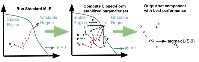
Figure 1: Diagram of the two-dimensional stabilization procedure. Given values for M and $\epsilon$, the algorithm consists in finding (M+1) points inside the stable region for the two-dimensional parameter vector $\theta$, each at a distance $\epsilon$ from the boundary. The (M+1) points represent a gradual change of the relevance of each component of $\theta$ to the its final stabilized value. The procedure for higher-dimensional $\theta$ follows analogously.

4 Experiments

For an initial empirical validation of the proposed stabilization strategy, we performed experiments with synthetic data generated from each of the five parametric forms. Since last iterate $\theta^{I}\in\Omega_{\epsilon}$, then clearly $\max_{\theta\in\Omega_{\epsilon}}\mathcal{L}(\theta,\mathcal{S})\geq\mathcal{L}(\theta^{I},\mathcal{S})$. Our goal is, then, verifying the rate with which the stabilization algorithm output strictly outperforms $\theta^{I}$, including those cases of model misassignment (e.g., an exponential kernel is used to fit a sequence generated by a gaussian kernel, and so on).

In the following, we investigate the performance of the stabilization algorithm over sequences of several different horizons T, and also verify the influence of margin parameter $\epsilon$ and stabilization resolution M on the success rate of stabilized kernels. The results are shown in Figure 2. The MLE optimization procedure is carried out with the standard Nelder-Mead method implementation from the Python SciPy library. As an example, a success rate of 0.9 for EXP kernel fitted over sequences generated with GSS kernels means that the likelihood of the parameters returned by the stabilization method is strictly higher than the original MLE last iterate $\theta^{I}$ in 90 % of the corresponding sequences. It can be observed that the MLE-STAB improves the performance of the model over a wide range of parameters, even in the case of kernel misassignment.

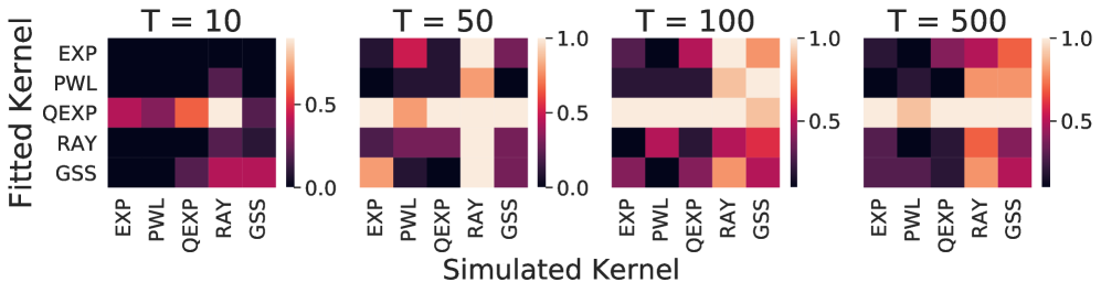
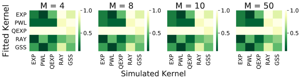
(a) Influence of T.

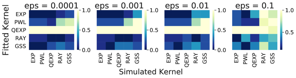
(b) Influence of M.

(c) Influence of $\epsilon$.

Figure 2: Influence of different parameters on the performance of the performance of the MLE-STAB algorithm.

4.1 Baseline Comparisons on Real and Synthetic Data

For testing the quality of our stabilization algorithms, hereby denoted MLE- STAB, we performed experiments with real data. The chosen datasets were "Hawkes","Retweet" and "Missing". Their description and content can be found in (Mei & Eisner (2017)). The baselines chosen were those which allowed for a more flexible modeling of the triggering function. They are the implementations of HawkesEM, HawkesBasisKernels and HawkesConditionalLaw, publicly available in the tick library (Bacry et al. (2017)).

Dataset /Method	MLE-STAB	HawkesEM
Hawkes	5.30	0.039
Missing	5.27	-0.06
Retweet	71.29	-20.68

Table 1: Comparison of the stabilization method with baseline over standardized datasets. The result shown corresponds to the average, across all sequences, of the loglikelihood of the method on the test portion of the given sequence (final $30\%$ of the event horizon $[0,T]$). The loglikelihood is normalized by the number of events contained in this given test portion.

We intend to show here that, for most real-world applications, the number of events associated with a given self-triggering dynamics is usually small. This fact is advantageous to simple parametric functions, such as the ones we presented here. And the improvements proposed by the MLE-STAB algorithm works on improving the predictive power of these simpler parametric models. The models are fitted in the events up to $70\%$ of T, here taken as the time of the last event. And then have their loglikelihood evaluated in the final $30\%$. Unfortunately, the very small number of events was prohibitive for the HawkesBasisKernels and HawkesConditionalLaw models, thus only results for HawkesEM and MLE-STAB are displayed. The final average across all sequences of the dataset is shown in Table 1.

5 Conclusions

Hawkes Processes are particularly suited for modeling self- and mutually exciting interactions of discrete events in continuous-time event streams, what corroborates the increasing popularity they have enjoyed across many domains, such as Social Network analysis and High-Frequency Finance. A Maximum Likelihood Estimation (MLE) unconstrained optimization procedure over parametrically assumed forms of the triggering kernels of the corresponding intensity function are a widespread cost-effective modeling strategy, particularly suitable for data with few and/or short sequences. However, the MLE optimization lacks guarantees, except for strong assumptions on the parameters of the triggering kernels, and may lead to instability of the resulting parameters . In the present work, we show how a simple stabilization procedure improves the performance of the MLE optimization without these overly restrictive assumptions, while also accounting for model misassignment cases. This stabilized version of the MLE is shown to outperform the standard method over sequences of several different lengths. The effects of resolution and margin parameters are also evaluated, as well as baseline comparisons over standardized datasets.

Appendix A Appendix

A.1 Closed-Form Computation of $\Omega_{\epsilon}$ for Parametric Hawkes Processes

In this subsection, we detail the closed-form calculations of the stabilized parameter set $\Omega_{\epsilon}$ for each of the parametric forms for $\phi(t)$ detailed at Section 2.

A.1.1 Example 1: Closed-Form Stabilization of EXP($\alpha$,$\beta$)

For $\phi(t)=EXP(\alpha,\beta)$, we have $\theta^{I}=(\alpha^{I},\beta^{I})\in\mathbb{R}_{2}^{+}$. By defining M, $\epsilon$, j = 1 and k = 2, with $\alpha=\theta^{1}$, $\beta=\theta^{2}$ and $|\phi|=\int_{0^{-}}^{\infty}\phi(t)$, we can find tuples ($\alpha^{\prime}$,$\beta^{\prime}$) such that:

$$\dfrac{\alpha^{\prime}}{\beta^{I}}=|\phi|^{\dfrac{M-i}{M}}/(1+\epsilon)^{\dfrac{i}{M}}\;\;\;\;\;\;\;\;\;\;\;\;\;\;\;\dfrac{\alpha^{I}}{\beta^{\prime}}=|\phi|^{\dfrac{i}{M}}/(1+\epsilon)^{\dfrac{M-i}{M}}\;\;\;\;\;\;\;\;\;\;\;\;\;\;\;\dfrac{\alpha^{I}}{\beta^{I}}=|\phi|,$$ (5)

for each value of $i\in\{0,1,...,M\}$ as given in Equation 4. From that, we can readily find:

$$\Omega_{\epsilon}=\{(\alpha^{I},\beta^{I})\}\cup\{(\alpha^{I}/(|\phi|(1+\epsilon))^{\dfrac{i}{M}}),\beta^{I}(|\phi|(1+\epsilon))^{\dfrac{M-i}{M}})\}_{i=0}^{M}$$ (6)

A.1.2 Example 2: Closed-Form Stabilization of PWL(K,c,p)

For $\phi(t)=PWL(K,c,p)$, we have $\theta^{I}=(K^{I},c^{I},p^{I})\in\mathbb{R}_{3}^{+}$. By defining M, $\epsilon$, j = 1 and k = 2, with $K=\theta^{1}$ and $c=\theta^{2}$, we can readily find:

$$\Omega_{\epsilon}=\{(K^{I},c^{I},p^{I})\}\cup\{(K^{I}/(|\phi|(1+\epsilon))^{\dfrac{i}{M}},c^{I}((|\phi|(1+\epsilon))^{\dfrac{M-i}{M}})^{\frac{1}{p^{I}-1}},p^{I})\}_{i=0}^{M}$$ (7)

By defining j = 1 and k = 3, with $K=\theta^{1}$ and $p=\theta^{3}$, we can readily find:

$$\Omega_{\epsilon}=\{(K^{I},c^{I},p^{I})\}\cup{(K^{I}/(|\phi|(1+\epsilon)),c^{I},p^{I})}\cup\{(K^{I}/(|\phi|(1+\epsilon))^{\dfrac{i}{M}},c^{I},1+\frac{W(\Delta^{i}\log c^{I})}{\log c^{I}})\}_{i=0}^{M-1}$$ (8)

where

$$\Delta^{i}=(|\phi|(1+\epsilon))^{\dfrac{M-i}{M}}(p^{I}-1){c^{I}}^{(p^{I}-1)}$$ (9)

and W is a standard function, taken as the analytical continuation of branch 0 of the product log (Lambert-W) function.

A.1.3 Example 3: Closed-Form Stabilization of QEXP(a,q)

For $\phi(t)=QEXP(a,q)$, we have $\theta^{I}=(a^{I},q^{I})\in\mathbb{R}_{2}^{+}$. By defining M, $\epsilon$, j = 1 and k = 2, with $a=\theta^{1}$, $q=\theta^{2}$ and $|\phi|=\int_{0^{-}}^{\infty}\phi(t)$, we can readily find:

$$\Omega_{\epsilon}=\{(a^{I},q^{I})\}\cup\{(\frac{a}{(|\phi|(1+\epsilon)})^{\dfrac{i}{M}},2-(2-q)(|\phi|(1+\epsilon))^{\dfrac{M-i}{M}})\}_{i=0}^{M}$$ (10)

A.1.4 Example 4: Closed-Form Stabilization of RAY($\gamma$,$\eta$)

For $\phi(t)=RAY(\gamma,\eta)$, we have $\theta^{I}=(\gamma^{I},\eta^{I})\in\mathbb{R}_{2}^{+}$. By defining M, $\epsilon$, j = 1 and k = 2, with $\gamma=\theta^{1}$, $\eta=\theta^{2}$ and $|\phi|=\int_{0^{-}}^{\infty}\phi(t)$, we can readily find:

$$\Omega_{\epsilon}=\{(\gamma^{I},\eta^{I})\}\cup\{(\gamma^{I}/(|\phi|(1+\epsilon))^{\dfrac{i}{M}}),\eta^{I}(|\phi|(1+\epsilon))^{\dfrac{M-i}{M}})\}_{i=0}^{M}$$ (11)

A.1.5 Example 5: Closed-Form Stabilization of GSS($\kappa$,$\tau$,$\sigma$)

For $\phi(t)=GSS(\kappa,\tau,\sigma)$, we have $\theta^{I}=(\kappa^{I},\tau^{I},\sigma^{I})\in\mathbb{R}_{3}^{+}$. By defining M, $\epsilon$, j = 1 and k = 2, with $\kappa=\theta^{1}$, $\tau=\theta^{2}$ and $|\phi|=\int_{0^{-}}^{\infty}\phi(t)$, we can readily find:

$$\begin{split}\Omega_{\epsilon}=&\{(\kappa^{I},\tau^{I},\sigma^{I})\}\cup\{(\kappa^{I}/(|\phi|(1+\epsilon))^{\dfrac{i}{M}},\tau^{I}\dfrac{\operatorname{erfinv}{(2/(\kappa\sqrt{\pi\sigma}(1+\epsilon)^{\dfrac{M-i}{M}})-1})}{\operatorname{erfinv}{(2|\phi|^{\dfrac{M-i}{M}}/(\kappa\sqrt{\pi}\sqrt{\sigma})-1})},\sigma^{I})\}_{i=0}^{M-1}\\ &\cup\{(\kappa^{I}/(|\phi|(1+\epsilon)),\tau^{I},\sigma^{I})\},\end{split}$$ (12)

where erfinv is the inverse of the error function ($erf(z)=\dfrac{2}{\sqrt{\pi}}\int_{0}^{z}\mathrm{e}^{-x^{2}}dx$). In practice, the arguments of erfinv functions are constrained to be less than 1.

A.2 Related Works

The ubiquity of applicability of HPs has given rise to a myriad of modeling approaches for the triggering effect, inspired by parametric functions (e.g., Exponential, Power-Law, Gaussian) (Ozaki (1979); Xu et al. (2016); Liu et al. (2018)) and Gaussian Processes (Zhang et al. (2019b)). For data hungry applications, choices such as non-parametric methods (Yang et al. (2017); Bacry & Muzy (2016); Lewis & Mohler (2011); Zhang et al. (2019c)), Neural Networks (NN) (Mei & Eisner (2017); Du et al. (2016); Xiao et al. (2018); Omi et al. (2019); Shang & Sun (2019)), Attention Models (Zhang et al. (2019a); Zuo et al. (2020)), have been proposed. Furthermore, improvements regarding real-world data limitations and challenges are developed in (Shelton et al. (2018); Trouleau et al. (2019); Salehi et al. (2019)).

In the parametric approach, several forms have been proposed, such as Exponential (Hawkes (1971)), Power-Law (Zhao et al. (2015); Bacry et al. (2016)), Rayleigh (Lima & Choi (2018)), Tsallis Q-Exponential (Lima & Choi (2018)) and Gaussian (Wang et al. (2020)). An additional, recently introduced, parametric modeling choice, the Mittag-Leffler function (Chen et al. (2020)), which is not feasible for explicit gradient-based optimization, is left for future work.

A recent work (He et al. (2019)) proposes a Convex Conjugate approach to tackle the non-convexity of the likelihood function. Regarding the stability of parameters, (Karabash (2013)) performs a theoretical analysis of unstable HPs, while (Jaisson & Rosenbaum (2015); Bacry et al. (2012b)) point to HPs with nearly unstable parameter as suitable for some application domains. Nevertheless, (Jaisson & Rosenbaum (2015)) restricts itself to the normalization of exponential kernel by its amplitude parameter, while (Bacry et al. (2012b)) concerns itself uniquely with asymptotic results, i.e., when the sequence of events is observed for a time window $[0,T]$, with $(T\rightarrow\infty)$. The work closest to ours is the one in (Lima & Choi (2018)), which can be shown to be a particular case of our algorithm, for a specific value of the Stabilization Resolution (SR) parameter (M=2).

A.3 Performance across different optimization methods

For verifying the performance of the stabilization algorithms beyond the default choice of Nelder-Mead method, we computed the average loglikelihood improvement for each kernel type across the following optimization methods: Nelder-Mead, Conjugate Gradient (CG), BFGS, L-BFGS-B, TNC, COBYLA and SLSQP.

All the methods were run with the default SciPy implementations, and the routines resulting in overflow were ignored. The parameters used were: T = 100, $\epsilon$ = 0.1 and M = 6. The results are shown in Table 2. The stabilization method shows increase in performance across all methods but CG.

Method	Nelder-Mead	CG	BFGS	L-BFGS-B	TNC	COBYLA	SLSQP
$\Delta\mathcal{L}$	+520.86	+0.0	+131.83	+124.57	+202.65	+682.47	+109.45

Table 2: Comparison of the stabilization method among different optimization methods. $\Delta\mathcal{L}$ is the average difference in loglikelihood among the stabilized kernel and the original last iterate kernel across all sequences.

The kernel types with largest increase in performance were EXP and QEXP.

A.4 Experimental Reproducibility Guidelines

For experiments with synthetic data, we performed experiments with sequences generated from each of the five parametric forms, with $\mu$ set as 0.5, and parameter values:

$$EXP(1.0,1.1)\;\;\;\;PWL(0.9,1.0,2.0)\;\;\;\;QEXP(0.8,1.1)\;\;\;\;RAY(1.2,1.0)\;\;\;\;GSS(0.5,0.5,1.0),$$ (13)

For the baseline comparison, initially, the chosen datasets were "Hawkes","Retweet" and "Missing", "Mimic" and "Meme". Their description and content can be found in (Mei & Eisner (2017)). For those datasets with more than one fold, only the first fold was used. Besides, only sequences with more than 20 events were considered. The "Meme" dataset had all sequences with a number of events which disallowed the fitting of all baselines, while "Mimic" dataset resulted in only one sequence being properly fitted for comparison. Thus, both these datasets were excluded from our comparison. After the model fitting, The loglikelihood of each sequence was then normalized by the number of events in the test portion. The performance of MLE-Stab is computed by choosing the parametric choice, out of the five possible ones, which performs best for each sequence.

References

- Bacry et al. (2012a) E. Bacry, K. Dayri, and J. F. Muzy. Non-parametric kernel estimation for symmetric hawkes processes. application to high frequency financial data. The European Physical Journal B, 85(5):1–12, 2012a.
- Bacry et al. (2017) E. Bacry, M. Bompaire, S. Gaïffas, and S. Poulsen. tick: a Python library for statistical learning, with a particular emphasis on time-dependent modeling. ArXiv e-prints, July 2017.
- Bacry & Muzy (2016) Emmanuel Bacry and Jean-François Muzy. First- and second-order statistics characterization of hawkes processes and non-parametric estimation. IEEE Trans. Information Theory, 62(4):2184–2202, 2016.
- Bacry et al. (2012b) Emmanuel Bacry, Sylvain Delattre, Marc Hoffmann, and J.F. Muzy. Scaling limits for hawkes processes and application to financial statistics. 123, 02 2012b.
- Bacry et al. (2015) Emmanuel Bacry, Iacopo Mastromatteo, and Jean-François Muzy. Hawkes processes in finance. arXiv, 2015.
- Bacry et al. (2016) Emmanuel Bacry, Thibault Jaisson, and Jean–François Muzy. Estimation of slowly decreasing hawkes kernels: application to high-frequency order book dynamics. Quantitative Finance, 16(8):1179–1201, 2016. doi: 10.1080/14697688.2015.1123287.
- Chen et al. (2020) Jing Chen, Alan G. Hawkes, and Enrico Scalas. A fractional hawkes process, 2020.
- Du et al. (2016) Nan Du, Hanjun Dai, Rakshit Trivedi, Utkarsh Upadhyay, Manuel Gomez-Rodriguez, and Le Song. Recurrent marked temporal point processes: Embedding event history to vector. In Proceedings of the 22nd ACM SIGKDD International Conference on Knowledge Discovery and Data Mining, San Francisco, CA, USA, August 13-17, 2016, 2016.
- Etesami et al. (2016) J. Etesami, N. Kiyavash, K. Zhang, and K. Singhal. Learning network of multivariate hawkes processes: A time series approach. In Proceedings of the Conference on Uncertainty in Artificial Intelligence, 2016.
- Hawkes (1971) Alan G. Hawkes. Spectra of some self-exciting and mutually exciting point processes. Biometrika, (1):201–213, 1971.
- He et al. (2019) Niao He, Zaid Harchaoui, Yichen Wang, and Le Song. Point process estimation with mirror prox algorithms. Applied Mathematics & Optimization, 2019. doi: 10.1007/s00245-019-09634-6.
- Helmstetter & Sornette (2002) A. Helmstetter and D. Sornette. Diffusion of epicenters of earthquake aftershocks, omori’s law, and generalized continuous-time random walk models. Phys. Rev. E, 66:061104, 2002.
- Jaisson & Rosenbaum (2015) Thibault Jaisson and Mathieu Rosenbaum. Limit theorems for nearly unstable hawkes processes. The Annals of Applied Probability, 25(2):600–631, 04 2015. URL https://doi.org/10.1214/14-AAP1005.
- Karabash (2013) Dmytro Karabash. On stability of hawkes process. 1 2013.
- Lewis & Mohler (2011) Erik Lewis and George Mohler. A nonparametric em algorithm for multiscale hawkes processes. Journal of Nonparametric Statistics, 1(1):1–20, 2011.
- Lima & Choi (2018) Rafael Lima and Jaesik Choi. Hawkes process kernel structure parametric search with renormalization factors, 2018.
- Linderman & Adams (2014) Scott W. Linderman and Ryan P. Adams. Discovering latent network structure in point process data. In Proceedings of the International Conference on Machine Learning, pp. 1413–1421, 2014.
- Liu et al. (2018) Yanchi Liu, Tan Yan, and Haifeng Chen. Exploiting graph regularized multi-dimensional hawkes processes for modeling events with spatio-temporal characteristics. In Proceedings of the 27th International Joint Conference on Artificial Intelligence, pp. 2475–2482. AAAI Press, 2018.
- Mei & Eisner (2017) Hongyuan Mei and Jason Eisner. The neural hawkes process: A neurally self-modulating multivariate point process. In Advances in Neural Information Processing Systems 30: Annual Conference on Neural Information Processing Systems 2017, 4-9 December 2017, Long Beach, CA, USA, 2017.
- Mohler et al. (2012) George O. Mohler, Martin B. Short, P. Jeffrey Brantingham, Frederic P. Schoenberg, and George E. Tita. Self-exciting point process modelling of crime. Journal of the American Statistical Association, 106(493):100–108, 2012.
- Ogata (1981) Yosihiko Ogata. On lewis’ simulation method for point processes. IEEE Transactions on Information Theory, 27(1):23–31, 1981.
- Omi et al. (2019) Takahiro Omi, Naonori Ueda, and Kazuyuki Aihara. Fully neural network based model for general temporal point processes. In Hanna M. Wallach, Hugo Larochelle, Alina Beygelzimer, Florence d’Alché-Buc, Emily B. Fox, and Roman Garnett (eds.), Advances in Neural Information Processing Systems 32: Annual Conference on Neural Information Processing Systems 2019, NeurIPS 2019, 8-14 December 2019, Vancouver, BC, Canada, pp. 2120–2129, 2019.
- Ozaki (1979) T. Ozaki. Maximum likelihood estimation of hawkes’ self-exciting point processes. Annals of the Institute of Statistical Mathematics, (31):145–155, 1979.
- Rizoiu et al. (2018a) Marian-Andrei Rizoiu, Young Lee, and Swapnil Mishra. Hawkes processes for events in social media. In Frontiers of Multimedia Research, pp. 191–218. 2018a.
- Rizoiu et al. (2018b) Marian-Andrei Rizoiu, Swapnil Mishra, Quyu Kong, Mark James Carman, and Lexing Xie. Sir-hawkes: Linking epidemic models and hawkes processes to model diffusions in finite populations. In Proceedings of the 2018 World Wide Web Conference on World Wide Web, WWW 2018, Lyon, France, April 23-27, 2018, pp. 419–428. ACM, 2018b.
- Salehi et al. (2019) Farnood Salehi, William Trouleau, Matthias Grossglauser, and Patrick Thiran. Learning hawkes processes from a handful of events. In Advances in Neural Information Processing Systems 32: Annual Conference on Neural Information Processing Systems 2019, NeurIPS 2019, 8-14 December 2019, Vancouver, BC, Canada, pp. 12694–12704, 2019.
- Shang & Sun (2019) Jin Shang and Mingxuan Sun. Geometric hawkes processes with graph convolutional recurrent neural networks. In The Thirty-Third AAAI Conference on Artificial Intelligence, AAAI 2019, Honolulu, Hawaii, USA, January 27 - February 1, 2019, pp. 4878–4885. AAAI Press, 2019.
- Shelton et al. (2018) Christian Shelton, Zhen Qin, and Chandini Shetty. Hawkes process inference with missing data, 2018.
- Trouleau et al. (2019) William Trouleau, Jalal Etesami, Matthias Grossglauser, Negar Kiyavash, and Patrick Thiran. Learning hawkes processes under synchronization noise. In Proceedings of the 36th International Conference on Machine Learning, ICML 2019, 9-15 June 2019, Long Beach, California, USA, volume 97 of Proceedings of Machine Learning Research, pp. 6325–6334. PMLR, 2019.
- Wang et al. (2020) Haoyun Wang, Liyan Xie, Alex Cuozzo, Simon Mak, and Yao Xie. Uncertainty quantification for inferring hawkes networks, 2020.
- Xiao et al. (2016) Shuai Xiao, Junchi Yan, Changsheng Li, Bo Jin, Xiangfeng Wang, Xiaokang Yang, Stephen M. Chu, and Hongyuan Zha. On modeling and predicting individual paper citation count over time. In Proceedings of the Twenty-Fifth International Joint Conference on Artificial Intelligence, IJCAI 2016, New York, NY, USA, 9-15 July 2016, pp. 2676–2682, 2016.
- Xiao et al. (2018) Shuai Xiao, Hongteng Xu, Junchi Yan, Mehrdad Farajtabar, Xiaokang Yang, Le Song, and Hongyuan Zha. Learning conditional generative models for temporal point processes. In Proceedings of the Thirty-Second AAAI Conference on Artificial Intelligence, (AAAI-18), the 30th innovative Applications of Artificial Intelligence (IAAI-18), and the 8th AAAI Symposium on Educational Advances in Artificial Intelligence (EAAI-18), New Orleans, Louisiana, USA, February 2-7, 2018, pp. 6302–6310, 2018.
- Xu et al. (2016) Hongteng Xu, Mehrdad Farajtabar, and Hongyuan Zha. Learning granger causality for hawkes processes. In Proceedings of the International Conference on Machine Learning, pp. 1717–1726, 2016.
- Yang et al. (2017) Yingxiang Yang, Jalal Etesami, Niao He, and Negar Kiyavash. Online learning for multivariate hawkes processes. In Advances in Neural Information Processing Systems 30: Annual Conference on Neural Information Processing Systems 2017, 4-9 December 2017, Long Beach, CA, USA, pp. 4944–4953, 2017.
- Zhang et al. (2019a) Qiang Zhang, Aldo Lipani, Ömer Kirnap, and Emine Yilmaz. Self-attentive hawkes processes. CoRR, abs/1907.07561, 2019a.
- Zhang et al. (2019b) Rui Zhang, Christian J. Walder, and Marian-Andrei Rizoiu. Sparse gaussian process modulated hawkes process. CoRR, abs/1905.10496, 2019b.
- Zhang et al. (2019c) Rui Zhang, Christian J. Walder, Marian-Andrei Rizoiu, and Lexing Xie. Efficient non-parametric bayesian hawkes processes. In Sarit Kraus (ed.), Proceedings of the Twenty-Eighth International Joint Conference on Artificial Intelligence, IJCAI 2019, Macao, China, August 10-16, 2019, pp. 4299–4305. ijcai.org, 2019c.
- Zhao et al. (2015) Qingyuan Zhao, Murat A. Erdogdu, Hera Y. He, Anand Rajaraman, and Jure Leskovec. Seismic: A self-exciting point process model for predicting tweet popularity. In Proceedings of the ACM SIGKDD International Conference on Knowledge Discovery and Data Mining, pp. 1513–1522, 2015.
- Zuo et al. (2020) Simiao Zuo, Haoming Jiang, Zichong Li, Tuo Zhao, and Hongyuan Zha. Transformer hawkes process. CoRR, abs/2002.09291, 2020. URL https://arxiv.org/abs/2002.09291.