AnomalyHop: An SSL-based Image Anomaly Localization Method

Abstract

An image anomaly localization method based on the successive subspace learning (SSL) framework, called AnomalyHop, is proposed in this work. AnomalyHop consists of three modules: 1) feature extraction via successive subspace learning (SSL), 2) normality feature distributions modeling via Gaussian models, and 3) anomaly map generation and fusion. Comparing with state-of-the-art image anomaly localization methods based on deep neural networks (DNNs), AnomalyHop is mathematically transparent, easy to train, and fast in its inference speed. Besides, its area under the ROC curve (ROC-AUC) performance on the MVTec AD dataset is 95.9%, which is among the best of several benchmarking methods.

I Introduction

Image anomaly localization is a technique that identifies the anomalous region of input images at the pixel level. It finds real-world applications such as manufacturing process monitoring [1], medical image diagnosis [2, 3] and video surveillance analysis [4, 5]. It is often assumed that only normal (i.e., anomaly-free) images are available in the training stage since anomalous samples are few to be modeled effectively rare and/or expensive to collect.

There is a growing interest in image anomaly localization due to the availability of a new dataset called the MVTec AD [6] (see Fig. 1). State-of-the-art image anomaly localization methods adopt deep learning. Many of them employ complicated pretrained neural networks to achieve high performance yet without a good understanding of the basic problem. To get marginal performance improvements, fine-tuning and other minor modifications are made on a try-and-error basis. Related work will be reviewed in Sec. II.

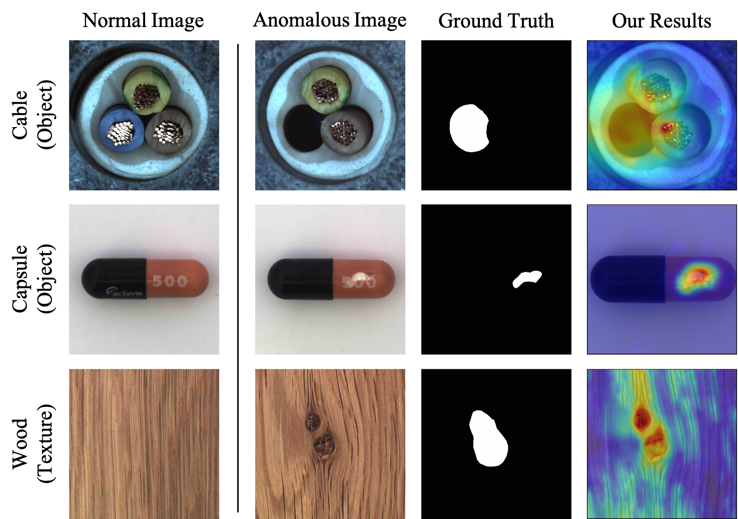
Figure 1: Image anomaly localization examples taken from the MVTec AD dataset (from left to right): normal images, anomalous images, the ground truth and the predicted anomalous region by AnomalyHop, where the red region indicates the detected anomalous region.

A new image anomaly localization method, called AnomalyHop, based on the successive subspace learning (SSL) framework is proposed in this work. This is the first work that applies SSL to the anomaly localization problem. AnomalyHop consists of three modules: 1) feature extraction via successive subspace learning (SSL), 2) normality feature distributions modeling via Gaussian models, and 3) anomaly map generation and fusion. They will be elaborated in Sec. III. As compared with deep-learning-based image anomaly localization methods, AnomalyHop is mathematically transparent, easy to train, and fast in its inference speed. Besides that, as reported in Sec. IV, its area under the ROC curve (ROC-AUC) performance on the MVTec AD dataset is 95.9%, which is the state-of-the-art performance. Finally, concluding remarks and possible future extensions will be given in Sec. V.

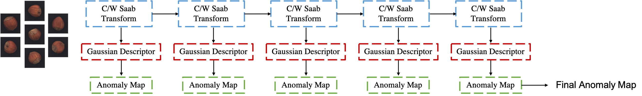
Figure 2: The system diagram of the proposed AnomalyHop method.

II Related Work

If the number of images in an image anomaly training set is limited, learning normal image features in local regions is challenging. We classify image anomaly localization methods into two major categories based on whether a method relies on external training data (say, the ImageNet) or not.

With External Training Data. Methods in the first category rely on pretrained deep learning models by leveraging external data. Examples include PaDiN [7], SPADE [8], DFR [9] and CNN-FD [4]. They employ a pretrained deep neural network (DNN) to extract local image features and, then, use various models to fit the distribution of features in normal regions. Although some offer impressive performance, they do rely on large pretrained networks such as the ResNet [10] and the Wide-ResNet [11]. Since these pretrained DNNs are not optimized for the image anomaly detection task, the associated image anomaly localization methods usually have large model sizes, high computational complexity and memory requirement.

Without External Training Data. Methods in the second category exploit neither pretrained DNNs nor external training data. They learn local image features based on normal images in the training set. For example, Bergmann et al. developed the MVTec AD dataset in [6] and used an autoencoder-like network to learn the representation of normal images. The network can reconstruct anomaly-free regions of high fidelity but not for anomalous regions. As a result, the pixel-wise difference between the input abnormal image and its reconstructed image reveals the region of abnormality. A similar idea was developed using the image inpainting technique [12, 13]. Traditional machine learning models such as support vector data description (SVDD) [14] can also be integrated with neural network, where novel loss terms are derived to learn local image features from scratch [15, 16]. Generally speaking, methods without external training data either fail to provide satisfactory performance or suffer from a slow inference speed [15]. This is attributed to diversified contents of normal images. For example, the 10 object classes and the 5 texture classes in the MVTec AD dataset are quite different. Their capability in representing features of local regions of different images is somehow limited. On the other hand, over-parameterized DNN models pretrained by external data may overfit some datasets but may not be generalizable to other unseen contents such as new texture patterns. It is desired to find an effective and mathematically transparent learning method to address this challenging problem.

SSL and Its Applications. SSL is an emerging machine learning technique developed by Kuo et al. in recent years [17, 18, 19, 20, 21]. It has been applied to quite a few applications with impressive performance. Examples include image classification [19, 20], image enhancement [22], image compression [23], deepfake image/video detection [24], point cloud classification, segmentation, registration [25, 26, 27, 28], face biometrics [29, 30], texture analysis and synthesis [31, 32], 3D medical image analysis [33], etc.

III AnomalyHop Method

AnomalyHop belongs to the second category of image anomaly localization methods. Its system diagram is illustrated in Fig. 2. It contains three modules: 1) feature extraction, 2) modeling of normality feature distributions, and 3) anomaly map generation. They will be elaborated below.

III-A SSL-based Feature Extraction

Deep-learning methods learn image features indirectly. Given a network architecture, the network learns the filter parameters first by minimizing a cost function end-to-end. Then, the network can be used to generate filter responses, and patch features are extracted as the filter responses at a certain layer. In contrast, the SSL framework extracts features of image patches directly using a data-driven approach. The basic idea is to study pixel correlations in a neighborhood (say, a patch) and use the principal component analysis (PCA) to define an orthogonal transform, also known as the Karhunen Loève transform (KLT). However, a single-stage PCA transform is not sufficient to obtain powerful features. A sequence of modifications have been proposed in [17, 18, 19, 20] to make the SSL framework complete.

The first modification is to build a sequence of PCA transforms in cascade with the max pooling inserted between two consecutive stages. The output of the previous stage serves as the input to the current stage. The cascaded transforms are used to capture short-, mid- and long-range correlations of pixels in an image. Since the neighborhood of a graph is called a hop (e.g., 1-hop neighbors, 2-hop neighbors, etc.), each transform stage is called a hop [19]. However, a straightforward cascade of multi-hop PCAs does not work properly due to the sign confusion problem, which was first pointed out in [17]. The second modification is to replace the linear PCA with an affine transform that adds a constant-element bias vector to the PCA response vector [18]. The bias vector is added to ensure all input elements to the next hop are positive to avoid sign confusion. This modified transform is called the Saab (Subspace approximation with adjusted bias) transform. The input and the output of the Saab transform are 3D tensors (including 2D spatial components and 1D spectral components.) By recognizing that the 1D spectral components are uncorrelated, the third modification was proposed in [20] to replace one 3D tensor input with multiple 2D tensor inputs. This is named as the channel-wise Saab (c/w Saab) transform, and it greatly reduces the model size of the standard Saab transform. Here we employee c/w Saab transform as our feature extractor, where the output of c/w Saab transform will provide pixel-wise image local features automatically.

III-B Modeling of Normality Feature Distributions

We propose three Gaussian models to describe the distributions of features of normal images, which are extracted in Sec. III-A.

III-B1 Location-aware Gaussian Model

If the input images of an image class are well aligned in the spatial domain, we expect that features at the same location are close to each other. We use $X_{ij}^{n}$ to denote the feature vector extracted from a patch centered at location $(i,j)$ of a certain hop in the $n$th training image. By following [7], we model the feature vectors of patches centered at the same location $(i,j)$ by a multivariate Gaussian distribution, $\mathbb{N}(\mu_{ij},\Sigma_{ij})$. Its sample mean is $\mu_{ij}=N^{-1}\sum^{N}_{n=1}X_{ij}^{n}$ and its sample covariance matrix is

$$\Sigma_{ij}=(N-1)^{-1}\sum^{N}_{n=1}(X_{ij}^{n}-\mu_{ij})(X_{ij}^{n}-\mu_{ij})^{T}+\epsilon I,$$

where $N$ is the number of training images of an image class, $\epsilon$ is a small positive number, and $I$ denotes identity matrix. The term $\epsilon I$ is added to ensure that the sample covariance matrix is positive semi-definite.

III-B2 Location-Independent Gaussian Model

For images of the same texture class, they have strong self-similarity. Besides, they are often shift-invariant. These properties can be exploited for texture-related tasks [31, 34, 35]. For homogeneous fine-granular textures, we can use a single Gaussian model for all local image features at each hop and call it the location-independent Gaussian model. The model has its mean $\mu=(NHW)^{-1}\sum_{i,j,n}X_{ij}^{n}$ and its covariance matrix

$$\Sigma=(NHW-1)^{-1}\sum_{i,j,n}(X_{ij}^{n}-\mu_{ij})(X_{ij}^{n}-\mu_{ij})^{T}+\epsilon I,$$

where $N$ is the number of training images in one texture class, and $H$ and $W$ are pixel numbers along the height and the width of texture images.

III-B3 Self-reference Gaussian Model

Both location-aware and location-independent Gaussian models utilize all training images to capture the normality feature distributions. However, images of the same class may have intra-class variations, which location-aware and location-independent Gaussian models cannot capture well. One example is the grid class in the MVTec AD dataset. Different images may have different grid orientations and lighting conditions. To address this problem, we train a Gaussian model with the distribution of features from a single normal image and call it the self-reference Gaussian. Again, we compute the sample mean as $\mu=(HW)^{-1}\sum_{i,j}X_{ij}$ and the sample covariance matrix as

$$\Sigma=(HW-1)^{-1}\sum_{i,j}(X_{ij}-\mu)(X_{ij}-\mu)+\epsilon I.$$

For this setting, we only use normal images in the training set to determine the c/w Saab transform filters. The self-reference Gaussian model is learned from the test image at the testing time. For more discussion, we refer to Sec. IV.

III-C Anomaly Map Generation and Fusion

With learned Gaussian models, we use the Mahalanobis distance,

$$M(X_{ij})=\sqrt{(X_{ij}-\mu_{ij})\Sigma_{ij}^{-1}(X_{ij}-\mu_{ij})^{T}},$$

as the anomaly score to show the anomalous level of a corresponding patch. Higher scores indicate a higher likelihood to be anomalous. By calculating the scores over all locations of a hop, we form an anomaly map at each hop for an input test image. Finally, we re-scale all anomaly maps to the same spatial size and fuse them by weighting average to yield the final anomaly map.

IV Experiments

Dataset and Evaluation Metric. We evaluate our model on the MVTec AD dataset [6]. It has 5,354 images from 15 classes, including 5 texture classes and 10 object classes, collected from real-world applications. The resolution of input images ranges from 700$\times$700 to 1024$\times$1024. The training set consists of normal images only while the test set contains both normal and abnormal images. The ground truth of anomaly regions is provided for the evaluation purpose. The area under the receiver operating characteristics curve (AUC-ROC) [36, 6] is chosen to be the performance evaluation metric.

Experimental Setup and Benchmarking Methods. First, we resize images of different resolutions to the same resolution of $224\times 224$. Next, we apply the 5-stage Pixelhop++ to all classes for feature extraction as shown in Fig. 2. The spatial sizes, $b\times b$, and the number, $k$, of filters at each hop are searched in the range of $2\leq b\leq 7$ and $2\leq k\leq 5$, respectively. The $2\times 2$ max-pooling is used between hops. The optimal hyper-parameters at each hop are class dependent. A representative case for the leather class is given in Table I. The optimal hyper-parameters of all 15 classes can be found in our Github codes. We compare AnomalyHop against seven benchmarking methods. Four of them belong to the first category that leverages external datasets. They are PaDiM [7], SPADE [8], DFR [9] and CNN-FD [4]. Three of them belong to the second category that solely relies on images in the MVTec AD dataset. They are AnoGAN [2], VAE-grad [36] and Patch-SVDD [15].

TABLE I: The hyper-parameters of spatial sizes and numbers of filters at each hop for the leather class.

Hop Index	1	2	3	4	5
b	5	5	3	2	2
k	4	4	4	4	4

TABLE II: Performance comparison of image anomaly localization methods in terms of AUC-ROC scores for the MVTec AD dataset, where the best results in each category are marked in bold.

	Pretrained w/ External Data				w/o Pretraining
	PaDiM [7]	SPADE [8]	DFR [9]	CNN-FD [4]	AnoGAN [2]	VAE-grad [36]	Patch-SVDD [15]	AnomalyHop
Carpet	0.991	0.975	0.970	0.720	0.540	0.735	0.926	0.942∗
Grid	0.973	0.937	0.980	0.590	0.580	0.961	0.962	0.984⋆
Leather	0.992	0.976	0.980	0.870	0.640	0.925	0.974	0.991∗
Tile	0.941	0.874	0.870	0.930	0.500	0.654	0.914	0.932∗
Wood	0.949	0.885	0.930	0.910	0.620	0.838	0.908	0.903∗
Avg. of Texture Classes	0.969	0.929	0.946	0.804	0.576	0.823	0.937	0.950${}^{\ }$
Bottle	0.983	0.984	0.970	0.780	0.860	0.922	0.981	0.975⋄
Cable	0.967	0.972	0.920	0.790	0.780	0.910	0.968	0.904⋄
Capsule	0.985	0.990	0.990	0.840	0.840	0.917	0.958	0.965⋄
Hazelnut	0.982	0.991	0.990	0.720	0.870	0.976	0.975	0.971⋄
Metal Nut	0.972	0.981	0.930	0.820	0.760	0.907	0.980	0.956⋄
Pill	0.957	0.965	0.970	0.680	0.870	0.930	0.951	0.970⋄
Screw	0.985	0.989	0.990	0.870	0.800	0.945	0.957	0.960⋆
Toothbrush	0.988	0.979	0.990	0.770	0.900	0.985	0.981	0.982⋄
Transistor	0.975	0.941	0.800	0.660	0.800	0.919	0.970	0.981⋄
Zipper	0.985	0.965	0.960	0.760	0.780	0.869	0.951	0.966⋄
Avg. of Object Classes	0.978	0.976	0.951	0.769	0.826	0.928	0.967	0.963${}^{\ }$
Avg. of All Classes	0.975	0.960	0.949	0.781	0.743	0.893	0.957	0.959${}^{\ }$

AUC-ROC Performance. We compare the AUC-ROC scores of AnomalyHop and seven benchmarking methods in Table II. As shown in the table, AnomalyHop performs the best among all methods with no external training data. Although Patch-SVDD has close performance, especially for the object classes, its inference speed is significantly slower as shown in Table III. The best performance in Table II is achieved by PaDiM [7] that takes the pretrained 50-layer Wide ResNet as the feature extractor backbone. Its superior performance largely depends on the generalizability of the pretrained network. In practical applications, we often encounter domain-specific images, which may not be covered by external training data. In contrast, AnomalyHop exploits the statistical correlations of pixels in short-, mid- and long-range neighborhoods and obtain the c/w Saab filters based on PCA. It can tailor to a specific application domain using a smaller number of normal images. Furthermore, the Wide-ResNet-50-2 model has more than 60M parameters while AnomalyHop has only 100K parameters in PixelHop++, which is used for image feature extraction.

Three Gaussian models are adopted by AnomalyHop to handle different classes in Table II. Results obtained using location-aware, location-independent and self-reference Gaussian models are marked with ^⋄, ^∗, ^⋆, respectively. The object classes are well-aligned in the dataset so that the location-aware Gaussian model is more suitable. For texture classes (e.g. carpet and wood classes), the location-independent Gaussian model is the most favorable since the texture classes are usually homogeneous across the whole image. The location information is less relevant. The grid class is a special one. On one hand, the grid image is homogeneous across the whole image. On the other hand, different grid images have different rotations, lighting conditions and viewing angles as shown in Fig. 3. As a result, the self-reference Gaussian model offers the best result.

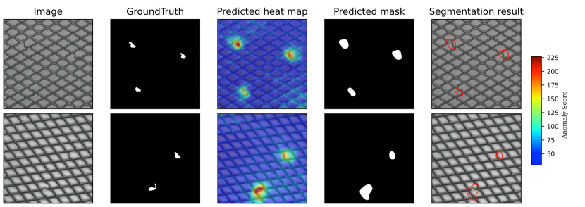
Figure 3: Two anomaly grid images (from left to right): input images, ground truth labels, predicted heatmap, predicted and segmented anomaly regions.

Inference Speed. The inference speed is another important performance metric in real-world image anomaly localization applications. We compare the inference speed of AnomalyHop and the other three high-performance methods in Table III, where all experiments are conducted with Intel I7-5930K@3.5GHz CPU. We see that AnomalyHop has the fastest inference speed. It has a speed-up factor of 4x, 22x and 28x with respect to PaDIM, Patch-SVDD and SPADE, respectively. SPADE and Patch-SVDD are significantly slower because of the expensive nearest neighbor search. For DNN-based methods, their feature extraction can be accelerated using GPU hardware, which applies to AnomalyHop, too. On the other hand, image anomaly localization is often conducted by edge computing devices in manufacturing lines. GPU could be too expensive for this environment. Although training complexity is often ignored since it has to be done once, it is worthwhile to mention that the training of AnomalyHop is very efficient. It takes only 2 minutes to train an AnomalyHop model for each class with the above-mentioned CPU.

TABLE III: Average inference time (in sec.) per image with Intel i7-5930K @ 3.5 GHz CPU.

Methods	Inference Time	Speed Up
SPADE [8]	6.80	1$\times$
Patch-SVDD [15]	5.23	1.3$\times$
PaDiM [7]	0.91	7.5$\times$
AnomalyHop	0.24	28.3$\times$

V Conclusion and Future Work

An SSL-based anomaly image localization method, called AnomalyHop, was proposed in this work. It is interpretable, effective and fast in both inference and training time. Besides, it offers state-of-the-art anomaly localization performance. AnomalyHop has a great potential to be used in a real-world environment due to its high performance as well as low implementation cost.

Although SSL-based feature extraction in AnomalyHop is powerful, its feature distribution modeling (module 2) and anomaly localization decision (module 3) are still primitive. These two modules can be improved furthermore. For example, it is interesting to leverage effective one-class classification methods such as SVDD [14], subspace SVDD [37] and multimodal subspace SVDD [38]. This is a new topic under our current investigation.

References

- [1] L. Scime and J. Beuth, “Anomaly detection and classification in a laser powder bed additive manufacturing process using a trained computer vision algorithm,” Additive Manufacturing, vol. 19, pp. 114–126, 2018.
- [2] T. Schlegl, P. Seeböck, S. M. Waldstein, U. Schmidt-Erfurth, and G. Langs, “Unsupervised anomaly detection with generative adversarial networks to guide marker discovery,” in International conference on information processing in medical imaging. Springer, 2017, pp. 146–157.
- [3] T. Schlegl, P. Seeböck, S. M. Waldstein, G. Langs, and U. Schmidt-Erfurth, “f-AnoGAN: Fast unsupervised anomaly detection with generative adversarial networks,” Medical image analysis, vol. 54, pp. 30–44, 2019.
- [4] P. Napoletano, F. Piccoli, and R. Schettini, “Anomaly detection in nanofibrous materials by cnn-based self-similarity,” Sensors, vol. 18, no. 1, p. 209, 2018.
- [5] V. Saligrama and Z. Chen, “Video anomaly detection based on local statistical aggregates,” in 2012 IEEE Conference on Computer Vision and Pattern Recognition. IEEE, 2012, pp. 2112–2119.
- [6] P. Bergmann, M. Fauser, D. Sattlegger, and C. Steger, “MVTec AD–A comprehensive real-world dataset for unsupervised anomaly detection,” in Proceedings of the IEEE/CVF Conference on Computer Vision and Pattern Recognition, 2019, pp. 9592–9600.
- [7] T. Defard, A. Setkov, A. Loesch, and R. Audigier, “PaDiM: a patch distribution modeling framework for anomaly detection and localization,” arXiv preprint arXiv:2011.08785, 2020.
- [8] N. Cohen and Y. Hoshen, “Sub-image anomaly detection with deep pyramid correspondences,” arXiv preprint arXiv:2005.02357, 2020.
- [9] J. Yang, Y. Shi, and Z. Qi, “DFR: Deep feature reconstruction for unsupervised anomaly segmentation,” arXiv preprint arXiv:2012.07122, 2020.
- [10] K. He, X. Zhang, S. Ren, and J. Sun, “Deep residual learning for image recognition,” in Proceedings of the IEEE conference on computer vision and pattern recognition, 2016, pp. 770–778.
- [11] S. Zagoruyko and N. Komodakis, “Wide residual networks,” in British Machine Vision Conference, 2016.
- [12] Z. Li, N. Li, K. Jiang, Z. Ma, X. Wei, X. Hong, and Y. Gong, “Superpixel masking and inpainting for self-supervised anomaly detection,” in 31st British Machine Vision Conference, 2020, pp. 7–10.
- [13] V. Zavrtanik, M. Kristan, and D. Skočaj, “Reconstruction by inpainting for visual anomaly detection,” Pattern Recognition, vol. 112, p. 107706, 2021.
- [14] D. M. Tax and R. P. Duin, “Support vector data description,” Machine learning, vol. 54, no. 1, pp. 45–66, 2004.
- [15] J. Yi and S. Yoon, “Patch svdd: Patch-level svdd for anomaly detection and segmentation,” in Proceedings of the Asian Conference on Computer Vision, 2020.
- [16] P. Liznerski, L. Ruff, R. A. Vandermeulen, B. J. Franks, M. Kloft, and K. R. Muller, “Explainable deep one-class classification,” in International Conference on Learning Representations, 2021.
- [17] C.-C. J. Kuo, “Understanding convolutional neural networks with a mathematical model,” Journal of Visual Communication and Image Representation, vol. 41, pp. 406–413, 2016.
- [18] C.-C. J. Kuo, M. Zhang, S. Li, J. Duan, and Y. Chen, “Interpretable convolutional neural networks via feedforward design,” Journal of Visual Communication and Image Representation, vol. 60, pp. 346–359, 2019.
- [19] Y. Chen and C.-C. J. Kuo, “Pixelhop: A successive subspace learning (ssl) method for object recognition,” Journal of Visual Communication and Image Representation, vol. 70, p. 102749, 2020.
- [20] Y. Chen, M. Rouhsedaghat, S. You, R. Rao, and C.-C. J. Kuo, “Pixelhop++: A small successive-subspace-learning-based (ssl-based) model for image classification,” in 2020 IEEE International Conference on Image Processing (ICIP). IEEE, 2020, pp. 3294–3298.
- [21] M. Rouhsedaghat, M. Monajatipoor, Z. Azizi, and C.-C. J. Kuo, “Successive subspace learning: An overview,” arXiv preprint arXiv:2103.00121, 2021.
- [22] Z. Azizi, X. Lei, and C.-C. J. Kuo, “Noise-aware texture-preserving low-light enhancement,” in 2020 IEEE International Conference on Visual Communications and Image Processing (VCIP). IEEE, 2020, pp. 443–446.
- [23] T.-W. Tseng, K.-J. Yang, C.-C. J. Kuo, and S.-H. Tsai, “An interpretable compression and classification system: Theory and applications,” IEEE Access, vol. 8, pp. 143 962–143 974, 2020.
- [24] H.-S. Chen, M. Rouhsedaghat, H. Ghani, S. Hu, S. You, and C.-C. J. Kuo, “Defakehop: A light-weight high-performance deepfake detector,” arXiv preprint arXiv:2103.06929, 2021.
- [25] M. Zhang, H. You, P. Kadam, S. Liu, and C.-C. J. Kuo, “Pointhop: An explainable machine learning method for point cloud classification,” IEEE Transactions on Multimedia, vol. 22, no. 7, pp. 1744–1755, 2020.
- [26] M. Zhang, Y. Wang, P. Kadam, S. Liu, and C.-C. J. Kuo, “Pointhop++: A lightweight learning model on point sets for 3d classification,” in 2020 IEEE International Conference on Image Processing (ICIP). IEEE, 2020, pp. 3319–3323.
- [27] M. Zhang, P. Kadam, S. Liu, and C.-C. J. Kuo, “Unsupervised feedforward feature (uff) learning for point cloud classification and segmentation,” in 2020 IEEE International Conference on Visual Communications and Image Processing (VCIP). IEEE, 2020, pp. 144–147.
- [28] P. Kadam, M. Zhang, S. Liu, and C.-C. J. Kuo, “R-pointhop: A green, accurate and unsupervised point cloud registration method,” arXiv preprint arXiv:2103.08129, 2021.
- [29] M. Rouhsedaghat, Y. Wang, S. Hu, S. You, and C.-C. J. Kuo, “Low-resolution face recognition in resource-constrained environments,” arXiv preprint arXiv:2011.11674, 2020.
- [30] M. Rouhsedaghat, Y. Wang, X. Ge, S. Hu, S. You, and C.-C. J. Kuo, “Facehop: A light-weight low-resolution face gender classification method,” arXiv preprint arXiv:2007.09510, 2020.
- [31] K. Zhang, H.-S. Chen, Y. Wang, X. Ji, and C.-C. J. Kuo, “Texture analysis via hierarchical spatial-spectral correlation (HSSC),” in 2019 IEEE International Conference on Image Processing (ICIP). IEEE, 2019, pp. 4419–4423.
- [32] X. Lei, G. Zhao, and C.-C. J. Kuo, “NITES: A non-parametric interpretable texture synthesis method,” in 2020 Asia-Pacific Signal and Information Processing Association Annual Summit and Conference (APSIPA ASC). IEEE, 2020, pp. 1698–1706.
- [33] X. Liu, F. Xing, C. Yang, C.-C. J. Kuo, S. Babu, G. E. Fakhri, T. Jenkins, and J. Woo, “Voxelhop: Successive subspace learning for als disease classification using structural mri,” arXiv preprint arXiv:2101.05131, 2021.
- [34] K. Zhang, H.-S. Chen, X. Zhang, Y. Wang, and C.-C. J. Kuo, “A data-centric approach to unsupervised texture segmentation using principle representative patterns,” in ICASSP 2019-2019 IEEE International Conference on Acoustics, Speech and Signal Processing (ICASSP). IEEE, 2019, pp. 1912–1916.
- [35] K. Zhang, B. Wang, H.-S. Chen, Y. Wang, S. Mou, and C.-C. J. Kuo, “Dynamic texture synthesis by incorporating long-range spatial and temporal correlations,” arXiv preprint arXiv:2104.05940, 2021.
- [36] D. Dehaene, O. Frigo, S. Combrexelle, and P. Eline, “Iterative energy-based projection on a normal data manifold for anomaly localization,” Internaltional Conference on Learning Representations, 2020.
- [37] F. Sohrab, J. Raitoharju, M. Gabbouj, and A. Iosifidis, “Subspace support vector data description,” in 2018 24th International Conference on Pattern Recognition (ICPR). IEEE, 2018, pp. 722–727.
- [38] F. Sohrab, J. Raitoharju, A. Iosifidis, and M. Gabbouj, “Multimodal subspace support vector data description,” Pattern Recognition, vol. 110, p. 107648, 2021.