Kudu: An Efficient and Scalable Distributed Graph Pattern Mining Engine

Abstract.

This paper proposes Kudu, a distributed execution engine with a well-defined abstraction that can be integrated with existing single-machine graph pattern mining (GPM) systems to provide efficiency and scalability at the same time. The key novelty is the extendable embedding abstraction which can express pattern enumeration algorithms, allow fine-grained task scheduling, and enable low-cost GPM-specific data reuse to reduce communication cost. The effective BFS-DFS hybrid exploration generates sufficient concurrent tasks for communication-computation overlapping with bounded memory consumption. Two scalable distributed GPM systems are implemented by porting Automine and GraphPi on Kudu. Our evaluation shows that Kudu based systems significantly outperform state-of-the-art distributed GPM systems with partitioned graphs by up to $75.5\times$ (on average $19.0\times$), achieve similar or even better performance compared with the fastest distributed GPM systems with replicated graph, and scale to massive graphs with more than one hundred billion edges with a commodity cluster.

1. Introduction

Graph pattern mining (GPM) (Teixeira et al., 2015), an important graph processing workload, is widely used in various applications (Ma’ayan, 2009; Schmidt et al., 2011; Wu et al., 2018; Valverde and Solé, 2005; Staniford-Chen et al., 1996; Juszczyszyn and Kołaczek, 2011; Becchetti et al., 2008). Given an input graph, GPM enumerates all its subgraphs isomorphic to some user-defined pattern(s), known as embeddings, and processes them to extract useful information. GPM application is computation intensive due to the need to enumerate an extremely large number of subgraphs. For example, there are more than 30 trillion edge-induced 6-chain embeddings on WikiVote (Leskovec et al., 2010)—a tiny graph with only 7K vertices. On the other side, the size of the graphs in real-world applications is continuously increasing. The importance and complexity of GPM applications give rise to the recent general GPM systems (Teixeira et al., 2015; Wang et al., 2018; Dias et al., 2019; Mawhirter and Wu, 2019; Jamshidi et al., 2020; Chen et al., 2020; Shi et al., 2020; Bindschaedler et al., 2021; Chen et al., 2018; Yan et al., 2020; Chen et al., 2021). In order to process large graphs efficiently, a GPM system should scale with both the computation and memory resources with good execution efficiency.

GPM can be performed with two approaches: (1) pattern-oblivious method—enumerating all subgraphs up to the pattern size and performing expensive isomorphic checks—used in early GPM systems such as Arabesque (Teixeira et al., 2015), Fractal (Dias et al., 2019), and RStream (Wang et al., 2018); and (2) pattern-aware enumeration method—generating the embeddings that match the patterns by construction without isomorphism checks—used in recent GPM systems such as Automine (Jamshidi et al., 2020), GraphZero (Mawhirter et al., 2021), Peregrine (Jamshidi et al., 2020), and GraphPi (Shi et al., 2020). This paper focuses on the pattern-aware enumeration due to its significantly better performance.

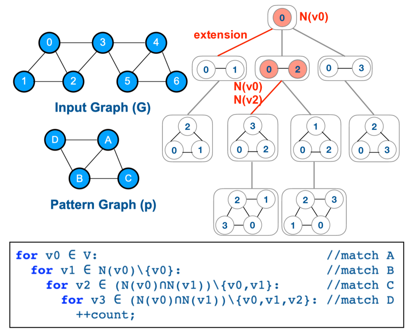
Figure 1. Pattern-aware Method and Embedding Tree

Figure 1 shows an example of the pattern-aware enumeration method. The nested loops construct the pattern embeddings in matching order (A,B,C,D), each loop level matches a vertex in the pattern graph. Such nested loops are executed from each vertex in the input graph. For each vertex $v0$, the code explores a tree structure with $v0$ as the root. Each tree node corresponds to a partially-constructed embedding or an embedding matching the pattern. Each tree level corresponds to a loop level. For example, the third loop (matching C) generates two tree nodes corresponding to three 2-vertex partially-constructed embedding ($v0$,$v2$,$v3$) and ($v0$,$v2$,$v1$) from ($v0$,$v2$). In general, a node needs to access an edge list ($N(v2)$ in above example) and perform intersections to generate a children. $N(v)$ is the edge list (neighbors) of $v$. We can see that the shape of the tree depends on the input graph. The tree leaves can be either embeddings matching the pattern, or subgraphs that cannot be extended further to match the pattern.

In a nutshell, the computation of GPM is to explore a massive number of trees (equal to the number of vertices in the input graph) based on the pattern graph and the input graph. We call such trees as embedding trees. The current GPM systems can be classified into two types based on whether remote data is accessed during the exploration of each embedding tree.

The first does not access remote edge lists during enumeration, including single-machine GPM systems, such as AutoMine (Mawhirter and Wu, 2019), Peregrine (Jamshidi et al., 2020), GraphZero (Mawhirter et al., 2021), Pangolin (Chen et al., 2020), and Sandslash (Chen et al., 2021), and distributed GPM systems with replicated graphs, such as Fractal (Dias et al., 2019), Arabesque (Teixeira et al., 2015), and GraphPi (Shi et al., 2020). The single-machine systems, which assume the input graph can fit into the memory, can support rudimentary out-of-core mode with memory mapped I/O to accommodate large graphs stored in disk but it may lead to poor performance for complicated patterns. RStream (Wang et al., 2018) is a specific out-of-core system that optimizes disk accesses, but it can only use the computation resource of one machine. The distributed systems scale with computation resources but the graph size is restricted by the memory of each machine.

The second type is distributed GPM systems with partitioned graphs, including G-miner (Chen et al., 2018) and its successor G-thinker (Yan et al., 2020), which access remote edge lists during enumeration. G-thinker and G-miner are designed with the “moving data to computation” policy. A recent distributed graph-querying system aDFS (Trigonakis et al., 2021) performs GPM tasks using an expressive SQL-like query language. It follows the “moving computation to data” policy that prevents many communication optimizations, leading to low performance for GPM tasks. For example, aDFS takes roughly 1000 seconds for triangle (size-3 complete subgraph) counting on the Friendster graph with 224 cores (Trigonakis et al., 2021) while AutoMine (Mawhirter and Wu, 2019) only takes roughly 400 seconds with 16 cores.

Tesseract (Bindschaedler et al., 2021) is a distributed GPM system optimized for dynamic graph updates, which stores the graph with a disaggregated key-value store. We do not consider it as a system with partitioned graphs. Its performance is not competitive compared to the state-of-the-art GPM systems: Tesseract takes 1.9 hours to mine all size-4 patterns on the LiveJournal (Leskovec et al., 2009) graph with eight 16-core machines (Bindschaedler et al., 2021) while GraphPi can perform the same task in 279 seconds with one machine.

Problem of G-thinker: We run experiments using the publicly available implementation. It takes 27.2s seconds for triangle counting on the Patents (Leskovec et al., 2005) graph on an 8-node cluster (8 cores per node) while a single-thread version finishes within 6.2 seconds (Mawhirter and Wu, 2019). The low performance of G-thinker is due to two reasons shown in Figure 2.

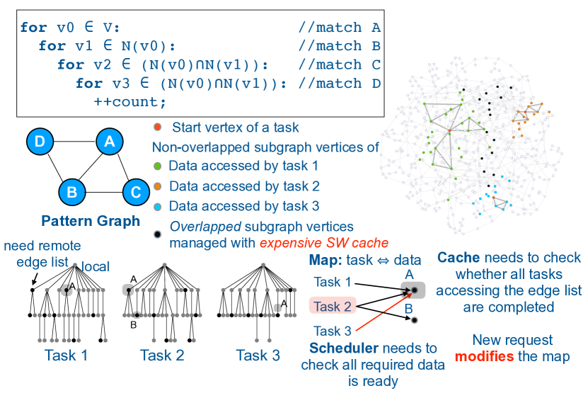
Figure 2. G-thinker: High Scheduler and Cache Overhead

• Limited parallelism. Each task of G-thinker explores an entire embedding tree. Each task of G-thinker explores an entire embedding tree. Before the computation, the task fetches a k-hop subgraph containing all necessary data for the tree exploration. Because the size of the k-hop subgraph increases quickly with k, the memory consumption of each task is large. Thus, the number of embedding trees that can be concurrently explored is reduced, e.g., about 150-300 trees for triangle counting on the Patents graph.

• General but expensive software cache and scheduler. To enable data reuse among tasks and avoid fetching the same edge list multiple times, G-thinker implements a software cache for remote edge lists management, which maintain a map between tasks and the dependent edge lists in cache, incurring high computation overhead. When a task requests an edge list of a vertex, the map needs to be updated. The scheduler periodically checks whether the edge lists needed by each task is ready. The cache periodically checks whether the tasks accessing an edge list are all completed, if so, it can be garbage collected.

Key idea: extendable embedding. We propose a novel abstraction that enables the efficient distributed execution of GPM algorithm. The key insight is to consider each extension as a fine-grained task. In an embedding tree (refer to Figure 1), each task corresponds to an edge in the tree from parent to its child, e.g., an edge between $(v0,v2)$ (parent) and $(v0,v2,v1)$ (child). Extendable embedding is the abstraction to realize such fine-grained tasks: an extendable embedding can be considered as a tree node—a partially-constructed embedding—together with some active edge lists, which are needed to perform the extension, i.e., generating the child. The extendable embedding for the tree node $(v0,v2)$ is $(v0,v2)$ plus $N(v0)$ and $N(v1)$, because the new vertex ($v1$ or $v3$) extended is identified by the intersection of $N(v0)$ and $N(v1)$. Extendable embedding is a well-defined abstraction that specifies the computation and the dependent data based on which the computation is performed. A fine-grained task performs the extension based on an extendable embedding after all active edge lists are fetched to local machine. In contrast, each task in G-thinker performs the exploration of a whole tree. The abstraction provides two important benefits illustrated in Figure 3.

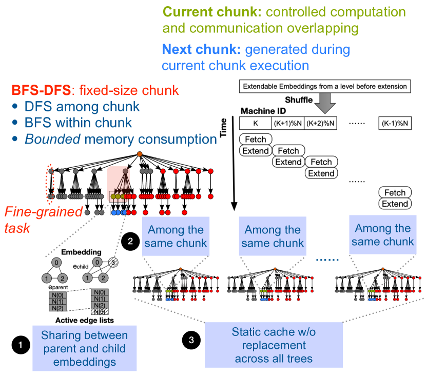
Figure 3. Benefits of Extendable Embedding Abstraction

Benefit 1: enabling flexible BFS-DFS hybrid exploration. The fine-grained task enabled by extendable embedding allows the flexible scheduling to take the best of BFS (high parallelism) and DFS (low memory consumption). We propose a BFS-DFS hybrid exploration with fixed-size extendable embedding chunks that performs DFS among chunks and BFS within a chunk. During the execution, the current chunk fills the next chunk until it is full. The hybrid approach bounds memory consumption because for each tree, we only need to allocate the memory of k chunks, where k is the level of tree nodes being explored. Before processing a chunk, we can shuffle the active edge lists based on the machine ID, and perform the computation and communication in a lightweight pipelined manner to maximize the chance of overlapping. While BFS-DFS exploration is also used in aDFS (Trigonakis et al., 2021), that system uses “moving computation to data” policy with poor performance for GPM.

Benefit 2: GPM-specific low-cost data reuse. Compared to the general software cache used in G-thinker, the fine-grained tasks enable three types of effective data reuse leveraging GPM algorithm properties. First, the data reuse between parent and child (❶): the child is extended with a new vertex from the parent, reuse of the shared data can be realized by pointers in the child to the parent. Second, data sharing among extendable embeddings in the same chunk (❷) can be realized by a simplified hash table. Third, the hot graph data can be kept in local machine by a static cache (❸). Unlike G-thinker, the static cache only inserts fetched edge list by certain criteria until it is full but never evicts data. It only reduces communication and remote edge lists access latency, but does not incur high overhead because the expensive bookkeeping that maintains the mapping between tasks and dependent edge lists is not needed.

The system: We built Kudu, the first distributed execution engine with a well-defined abstraction that can be conveniently integrated with existing single-machine GPM systems. This approach keeps the user-facing programming interface of existing systems unmodified, which typically specifies the pattern to mine, and only requires modest changes to the existing GPM systems’ implementations. Specifically, a GPM system developer can implement the pattern-specific subgraph enumeration, i.e., a sequence of extensions in the embedding tree shown in Figure 1, in a single EXTEND function, which is the sole interface between a single-machine GPM system and Kudu. Internally, Kudu implements a scheduler and execution model to realize the hybrid scheduling.

Experimental result highlights: We built two scalable and efficient distributed GPM systems, k-Automine and k-GraphPi, by porting Automine (Mawhirter and Wu, 2019) and GraphPi (Shi et al., 2020) on top of Kudu, with porting cost of roughly 500 lines of code per system. k-Automine and k-GraphPi significantly outperform G-thinker by up to $75.5\times$ and $75.5\times$ (on average $17.7\times$ and $20.3\times$), respectively. Compared to GraphPi, the fastest distributed GPM system with replicated graph, Kudu based systems show similar or even better performance compared and scale to massive graphs with more than one hundred billion edges that replication based systems cannot handle. More impressively, k-Automine even outperforms a state-of-the-art CPU-based distributed triangle counting implementation (Pearce, 2017) targeting large graphs.

Key lesson: Unless shared through the static cache, there is no sharing between two extendable embeddings of different trees, or different levels of the same tree if one is not the decedent of another. In contrast, G-thinker allows the sharing of all edge lists in the cache, which indeed translates to less communication between machines than Kudu. However, our approach leverages GPM-specific properties to enable low-cost data sharing and avoids the high overhead of G-thinker. Our results show that on average Kudu incurs about 3$\times$ communication of G-thinker but achieves average speedups of $19.0\times$ (up to $75.5\times$). Not solely focusing on one aspect and effectively exploring the trade-offs between overhead and communication amount, is the most important takeaway.

2. Background

2.1. Graph Mining Problem

A graph $G$ is defined as $G=(V,E)$, in which $V$ and $E$ are the set of graph vertices and edges. Similar to other systems (Teixeira et al., 2015; Chen et al., 2020; Mawhirter and Wu, 2019; Jamshidi et al., 2020), this paper considers undirected graphs, while the techniques are also applicable to directed graphs. We denote the vertex set containing $v$’s neighbors as $N(v)$. Each vertex or edge may have a label, and can be represented by a mapping $f_{L}:V\cup E\rightarrow L$ where $L$ is the label set. Currently, Kudu supports vertex labels, but the edge label support can be added without fundamental difficulty. Two graphs $G_{0}=(V_{0},E_{0})$ and $G_{1}=(V_{1},E_{1})$ are isomorphic iff. there exists a bijective function $f:V_{0}\rightarrow V_{1}$ such that $(u,v)\in E_{0}\iff(f(u),f(v))\in E_{1}$. Intuitively, isomorphic graphs have the same structure.

Given an input graph $G$, a GPM task discovers and processes $G$’s subgraphs that are isomorphic with a user-specified pattern $p$, which is a small connected graph reflecting some application-specific knowledge. The subgraphs matching (isomorphic with) $p$ is called $p$’s embeddings. In Figure 1, $G$’s subgraphs $e_{1}$ and $e_{2}$ are isomorphic to the pattern graph $p$.

2.2. Distributed Graph Pattern Mining

Graph partitioning divides graph data into multiple partitions, each of which is stored in the memory of one machine of a distributed cluster. Thus, the application can scale with both memory and compute resources. In this paper, we use 1-D graph partitioning: the vertices set $V$ of the input graph is partitioned into $N$ parts $V_{0},V_{1},\ldots,V_{N-1}$, where $N$ is the number of machines. Machine $i$ ($0\leq i<N$) maintains all graph data related to $V_{i}$—all edges with at least one endpoint in $V_{i}$—in its memory. To ensure balanced data distribution, similar to previous systems (Malewicz et al., 2010; Yan et al., 2020), the graph partitioning is determined by a hash function $H(v)$ that maps a vertex $v$ to its partition ID—an integer between $0$ and $N-1$. Figure 4 shows an example of input graph partitioning among three machines. Each machine contains a subset of vertices mapped to it and all edges that are connected to them.

With graph partition, the graph data needed in enumeration may not exist in the memory of the local machine—incurring remote data accesses and communication overhead. Such overhead can be exaggerated in the skewed graphs—the real-world graphs that follow the “power law”. Specifically, since the high-degree vertices with long edge lists belong to much more subgraphs and are more frequently accessed, the fetch of their edge lists can lead to a tremendous amount of communication.

2.3. Two Strategies for Distributed GPM

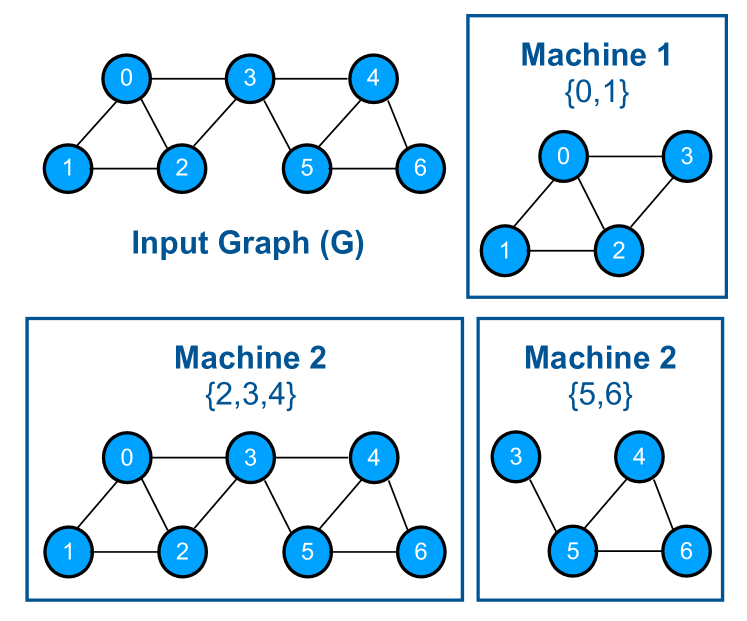
Figure 4. 1-D Partitioned Graph

Moving computation to data. This approach, originated from Arabesque (Teixeira et al., 2015), performs the extension (computation) at the machine which keeps the required data. The partially-constructed embeddings during pattern enumeration are transferred among machines. For the example in Figure 1 with graph partition of Figure 4, starting from $v0$, machine 1 first locally extends it into three subgraphs using local $N(0)$. For the next extension, subgraph $(v0,v1)$ requires $N(1)$, which is also local; while subgraph $(v0,v2)$ and $(v0,v3)$ require $N(2)$ and $N(3)$, which are stored in machine 2 according to the partition. Thus, subgraph $(v0,v2)$ and $(v0,v3)$ are sent to machine 2, together with $N(0)$ since it is needed for intersection between $N(2)$ and $N(3)$. After machine 2 receives these data, it performs local extension. The extension of subgraph $(v0,v1)$ is performed in machine 1 locally.

This approach has two drawbacks: (1) excessive communication overhead due to the transfer of additional edge lists for computation; and (2) difficult to reduce communication with data reuse. Its poor performance of aDFS (Trigonakis et al., 2021) on GPM confirms the drawbacks.

Moving data to computation. This approach, which is used by G-thinker (Yan et al., 2020), performs the embedding tree exploration from a given vertex $v$ in the machine that $v$ resides based on the input graph partition. For a graph with $|V|$ vertices, G-thinker performs enumeration with $|V|$ coarse-grained tasks for the $|V|$ embedding tree explorations. For each tree, the task first fetches a k-hop subgraph containing all data needed by its computation and then performs computation only after the k-hop subgraph is fetched to local machine. Thus, G-thinker can reduce communication by data reuse, which is impossible for “moving computation to data” because the data transferred is partially-constructed subgraphs.

The coarse-grained tasks of G-thinker limits the parallelism. Due to the high memory consumption of the k-hop subgraph, the number of tasks (or trees) explored concurrently is small (about several hundreds). Thus the capability that computation can be overlapped with communication is limited, which leads to low CPU utilization. It is confirmed by our experiments: for triangle counting on the Patents graph, G-thinker’s computation threads spend more than $70\%$ of runtime waiting for the communication thread to fetch remote data and update the software cache. More importantly, the map between task and data maintained by the cache incurs high overhead.

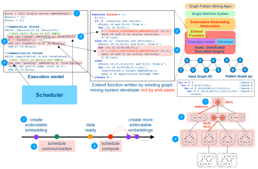
Figure 5. Extendable embedding: concept, execution model and scheduler

3. Key Abstraction: Extendable Embedding

3.1. Definitions

In pattern-aware enumeration, the embedding $e(p)$ matching a given pattern $p$ can be constructed by a sequence of extensions according to the pattern and the algorithm, which determines the order of the extensions. To emphasize that these subgraphs are enumerated in the process of constructing $e(p)$, we call the subgraphs enumerated in the sequence of extension also as embeddings (partially-constructed), which match part of $p$. Formally, each embedding $e(p)$ can be constructed by a sequence $e_{0}\rightarrow e_{1}\rightarrow...\rightarrow e(p)$, where $e_{0}$ is a single vertex.

When $e_{i}$ is extended to $e_{i+1}$, $e_{i}$ and $e_{i+1}$ are considered to be the parent ($e_{parent}$) and child ($e_{child}$) embedding. Based on the enumeration algorithm shown in Figure 1, extending $e_{parent}$ to $e_{child}$ requires the edge list of several active vertices in $e_{parent}$. The edge lists of active vertices are called active edge lists.

An extendable embedding is defined as a partially-constructed embedding $e_{i}$ in a tree node, along with active edge lists. Without confusion, we can also refer to an extendable embedding by $e_{i}$. With the data of an extendable embedding available, $e_{i}$ can be extended to $e_{i+1}$. The active vertices and edge lists are determined by the pattern graph and the pattern enumeration algorithm. Based on our definition, the “activeness” follows the anti-monoticity property: if a vertex in $e_{i}$ is inactive, then it must be also inactive in any $e_{j}$, where $j>i$. This property enables the succinct storage of extendable embeddings. In Figure 1, the extendable embedding for $(v0,v2)$ tree node is the subgraph itself with $v0$ and $v2$ being active vertices together with the edge lists of the two vertices: $N(v0)$ and $N(v2)$. Not all vertices in a partially-constructed embedding may be active. For example, the extendable embedding of tree node $(v0,v2,v3)$ has $v0$ and $v2$ (but not $v3$) as the active vertices and $N(v0)$ and $N(v2)$ as the active edge lists, because the next extension only requires the intersection of $N(v0)$ and $N(v2)$.

3.2. System Interface

Extendable embedding is the key abstraction to generate fine-grained tasks that can be scheduled efficiently leveraging the unique properties of pattern-aware enumeration algorithms. Specifically, with graph partitioned among distributed machines, when the data of an extendable embedding $e_{i}$ are all locally available, the machine can perform the computation to extend $e_{i}$ to $e_{i+1}$. As a result, extendable embedding breaks the embedding extension sequence to generate each $e(p)$ into fine-grained tasks with well-defined dependent data.

The interface exposed by Kudu to the client GPM systems is the EXTEND function. For a given pattern, the developer of a GPM system needs to express the implementations with nested loops in the EXTEND function based on the notion of extendable embedding. Figure 5 shows the an example of the EXTEND function for the nested loops enumerating pattern $p$ (on the right). The EXTEND function is called by the execution model (will be discussed next) with an extendable embedding as the parameter. Initially, all extendable embeddings are single vertices in the input graph.

We can see that the correspondence between the nested loop and the EXTEND function is intuitive: the EXTEND function executes different branches based on the current status of the extendable embedding. Each branch: (1) performs the extension based on the locally available active edge lists (ensured by the execution model); (2) uses the create_extendable _embedding() function to create a new extendable embedding ; (3) marks the active vertices and edges for the new extendable embedding; and (4) returns the new extendable embedding to the execution model, which will be responsible to fetch the remote active edge lists and schedule computation when they are ready.

The create_extendable_embedding() function is used to create an extendable embedding by adding one vertex to an existing embedding. The first two parameters of the function are the existing embedding and the new vertex. The third parameter represents the size of memory needed to store $e$’s reusable intermediate results (will be discussed in Section 5.1). Essentially, the EXTEND function breaks down the pattern enumeration algorithm into fine-grained computation (intersection) that can be flexibly scheduled by the execution model.

For a compilation-based single-machine GPM system, the generation of the EXTEND function for different patterns can be done by modifying the compiler, which originally generates the nested loop. We construct two distributed GPM systems by “porting” two compilation-based GPM systems, AutoMine (Mawhirter and Wu, 2019) and GraphPi (Shi et al., 2020), to Kudu in this manner. Thanks to the intuitive correspondence, the compiler modification is very modest: the porting effort is roughly 500 lines of codes per system. With the EXTEND function specified, Kudu engine can transparently orchestrate distributed execution. The client GPM system developers just need to focus on expressing pattern enumeration algorithm in the EXTEND function.

3.3. Execution Model

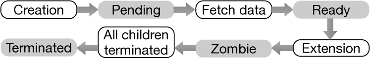
Figure 6. Extendable Embedding Execution States

The execution model maintains four states for each extendable embedding, shown in Figure 6. The “pending” state indicates that it has been created, but the active edge lists are not ready. In this state, the computation is waiting for data. The “ready” state means that the active edge lists have been fetched from either remote or local memory, and thus $e_{i}$ in the extendable embedding is ready to be extended to $e_{i+1}$. The embedding extension is scheduled when the computation resource is available. After the extension is performed, the state changes to “zombie”, which indicates that the extendable embedding’s computation is finished, but its memory resource cannot be released yet. It is because some data of the completed extendable embedding may be still shared with its children. When all children of an extendable embedding $e$ are completed, the state is changed to “terminated”, at which point the system can release the memory allocated to $e$. Thus, the extendable embeddings are deallocated in a “bottom-up” fashion.

Figure 5 (left) shows the execution model of Kudu. It specifies the operations performed by the computation and communication thread. The details to ensure thread-safety when multiple threads are used for computation and communication are discussed in Section 6. The set $E_{ready}$, $E_{pending}$, and $E_{zombie}$ contain the extendable embeddings in “ready”, “pending”, and “zombie” state, respectively. At the beginning, $E_{ready}$ is initialized to contain all single-vertex embeddings, because the embedding enumeration of any pattern needs to start from them. The other two sets are initialized as empty sets. The computation thread keeps popping “ready” extendable embeddings from $E_{ready}$ and extending them to larger ones. The EXTEND function will return a set of extended embedding $E^{\prime}$ if it has not reached the embedding of the pattern. Otherwise, the EXTEND function will return an empty set and call the user-defined function (UDF) to pass the identified embedding to the GPM application. After returning from the EXTEND function, newly generated extended embeddings in $E^{\prime}$ are added to $E_{pending}$, which will transparently trigger potential communication inside the execution model. For the current embedding $e^{\prime}$, since the extension has completed, it is added to $E_{zombie}$. We omit the details of keeping track of the children and state change from “zombie” to “terminated”.

The communication thread runs continuously until the end of application and executes whenever $E_{pending}$ is not empty. After popping one pending extendable embedding from $E_{pending}$, it fetches the data, either locally or from a remote machine. For local data, the communication thread just records the local data pointer. The remote data fetch is blocking, but we can batch multiple requests to amortize the network latency. After the communication is finished, the popped embedding from $E_{pending}$ is ready to be extended and added to $E_{ready}$,

3.4. Running Example

In this section, we describe several key steps in the EXTEND function and execution model based on the pattern graph $p$ in Figure 5. Initially, $E_{ready}$ contains all single-vertex embeddings in the local partition (❶) because the first extension step only needs the locally-available edge list these vertices. The task of GPM is to explore the embedding tree for all vertices in the local graph partition. The computation thread in the execution model will pick the extendable embeddings in $E_{ready}$ to perform extension. In ❷, the execution model takes an extendable embedding containing a single vertex $v0$ and its edge list $N(v0)$ and call the EXTEND function. We also mark the steps in the embedding tree on the right. Inside the EXTEND function, since $e^{\prime}$ just contains one vertex, the execution follows the first branch. A new extendable embedding is created for the extendable embedding: $v0$ extended with a neighbor vertex $v1$ corresponding to an edge in $N(v1)$. Before returning from the EXTEND function, $v0$ and $v1$ are marked as active vertices because $N(v0)$ and $N(v1)$ are needed for the next extension. In this example, the returned $E^{\prime}$ contains three extendable embeddings: $(v0,v1)$ with $N(v0)$ and $N(v1)$ as active edge lists; $(v0,v2)$ with $N(v0)$ and $N(v2)$ as active edge lists; and $(v0,v3)$ with $N(v0)$ and $N(v3)$ as active edge lists. They are inserted to the $E_{pending}$.

Based on the graph partition in Figure 4, $N(v2)$ and $N(v3)$ are stored in remote machine 2. Let us consider the extendable embedding $(v0,v2)$ with $N(v0)$ and $N(v2)$ as the example. Since $N(v2)$ is remote, the scheduler will later schedule the communication thread at some point to fetch the data (popped from $E_{pending}$ in ❸). The communication is blocking, and when $N(v2)$ arrives at the local machine, the extendable embedding is inserted into $E_{ready}$, which is ready to be scheduled for computation (intersection) by the computation thread. For $(v0,v1)$ with $N(v0)$ and $N(v1)$, because both required edge lists are local, there will be no communication incurred by the communication thread, and the computation will be scheduled directly.

In step ❹, the computation thread is scheduled to process the extendable embedding $(v0,v2)$ with $N(v0)$ and $N(v2)$ in $E_{ready}$. Similar to ❷, the execution model calls into the EXTEND function. This time, the extendable embedding contains two vertices $(v0,v2)$, so the execution falls into the second branch. New extendable embeddings are created for the extended embeddings found by the intersection of $N(v0)$ and $N(v2)$. In this example, two are generated: $(v0,v2,v3)$ with $N(v0)$ and $N(v2)$ as active edge lists, and $(v0,v2,v1)$ with $N(v0)$ and $N(v2)$ as active edge lists. Note that the active edge lists are the same since the next extension still performs the intersection between them.

On the second return from the EXTEND function, both $N(v0)$ and $N(v2)$ are local, so no communication is incurred to fetch $N(v2)$ again. In Kudu, it is realized by accessing the active edge lists in parent node ($(v0,v2)$) through pointers in child nodes ($(v0,v2,v3)$ and $(v0,v2,v1)$). The details are discussed in Section 5.1.

4. Hybrid Embedding Exploration

4.1. Motivation

With DFS exploration, the extendable embeddings of the same tree can be maintained by a stack with small memory consumption. The FILO order naturally satisfies the bottom-up memory release order. However, each tree only has one on-the-fly extendable embedding at any time—significantly limiting the capability of generating batched communication. One may consider exploring multiple DFS trees concurrently to provide sufficient parallelism for communication batching and overlapping. However, it does not solve the problem either. Due to the power law, there are a small number of large DFS trees with high-degree starting vertices and many small trees. In the beginning, the system can generate batched requests and overlap communication and computation because of plenty parallelism. Gradually, the DFSs of small trees quickly terminate, and there are only few large DFS trees left. Hence there are not sufficient batched requests and parallelism to hide the communication cost.

With BFS exploration, while sufficient number of on-the-fly extendable embeddings can be generated, the policy leads to inefficient memory management. The essential reason is that, extendable embeddings are not released in the order that they are allocated. Thus, different objects vary in size and lead to the fragmentation problem. In general, BFS tends to generate a very large number of embeddings—much larger than necessary for communication batching and overlapping—and results in enormous memory consumption.

4.2. BFS-DFS Hybrid Exploration

A chunk is defined as a configurable number of extendable embeddings of the same level. We propose to apply DFS at a chunk granularity while exploring embeddings in a BFS manner within a chunk. The memory of the chunk can be allocated and deallocated together to avoid fragmentation. Moreover, we can control the memory consumption with the chunk size. The data in the fixed memory for a chunk can be horizontally shared among its extendable embeddings. The lightweight mechanism to enable such sharing is discussed in Section 5.2.

The hybrid BFS-DFS scheduling ensures that, at any time, only one chunk of an embedding tree is being processed. The memory consumption is bounded since we just need to allocate the fixed memory for a chunk per level from the root to the current level being explored. On the other side, it eliminates the drawbacks of DFS since a chunk enables many on-the-fly extendable embeddings within it, which enables batched communication.

During execution, the current chunk in tree level-$i$ performs the extension and generates new extendable embeddings to be extended in the next chunk in tree level-$(i+1)$. Before filling the next chunk, a fixed amount of memory (e.g., 1GB memory) is pre-allocated. The next chunk is filled until the its memory is full. The procesure is shown in Figure 7. At the beginning, the current level is $i$, so we only extend level-$i$’s embeddings until the memory for level-$(i+1)$ is full. At this point, we stop the execution at level-$i$ and change level-$(i+1)$ as the current level. Thus, the current level keeps going deeper in until it reaches the deepest level that does not generate any new embeddings, then it backtracks to the previous level. Once the current level changes from level-$(i+1)$ to level-$i$, all level-$(i+1)$’s extendable embeddings can be released because all their descendants have been processed, and the execution of level-$i$ can resume. The DFS at chunk granularity repeats until all embeddings are enumerated.

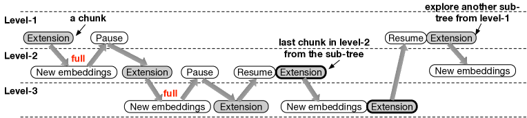
Figure 7. BFS-DFS Hybrid Exploration

4.3. Circulant Scheduling

For a chunk, communication and computation overlapping can be increased by circulant scheduling. As shown in Figure 3 (right), on machine $K$, once a level becomes full, before performing the extensions, the system shuffles all extendable embeddings at this level to $N$ batches according to the source machine ID in a circulant manner, where $N$ is the number of machines in the cluster. These batches contain the extendable embeddings whose active edge lists reside on machine $K$, $(K+1)\%N$, $(K+2)\%N$, $\ldots$, $0$, $\ldots$, $(K+N-1)\%N$, respectively. The key idea is to divide the execution of a chunk into multiple steps, and pipeline the execution and communication of the batches, so that in each step the computation of batch-$i$ is overlapped with the data fetch for batch-$(i+1)$. A communication batch is the data transfer between the local machine and one particular remote machine.

It is worth noting that we do not adopt the strict pipelining—the computation does not stall communication. For example, once the data required by batch-$i$ has been fetched, the system immediately starts the communication of batch-$(i+1)$ without waiting for the completion of batch-$(i-1)$’s computation.

5. Low-Cost Data Sharing

5.1. Vertical Data and Computation Sharing

During embedding tree exploration, different extendable embeddings may share common active edge lists. Specifically, if an extendable embedding $e_{child}$ is extended from $e_{parent}$, most active edge list data of $e_{child}$ are also included in $e_{parent}$. Figure 8 shows an example for 5-clique mining. Here, $e_{child}$ is obtained by extending $e_{parent}$ with $v3$, which should be one of the vertices in the intersection of $N(0)$, $N(1)$ and $N(2)$. To extend $e_{child}$, $N(3)$ is needed. Both $e_{child}$ and $e_{parent}$ include the active edge lists $N(0)$, $N(1)$ and $N(2)$, and $e_{child}$ only needs to additionally store $N(3)$ and refer $N(0)\sim N(2)$ to $e_{parent}$. Since there is only one active vertex of $e_{child}$ that is not included in $e_{parent}$, $e_{child}$ only needs to store the active edge list of one vertex. Such data reuse reduces the communication as well: for an extendable embedding $e_{child}$, only the edge list of the new vertex is fetched. Figure 8 (right) shows the hierarchical representation of tree nodes in $k$ levels. The extendable embeddings in level-$i$ have the same number of vertices, and point to the embeddings in level-$(i-1)$.

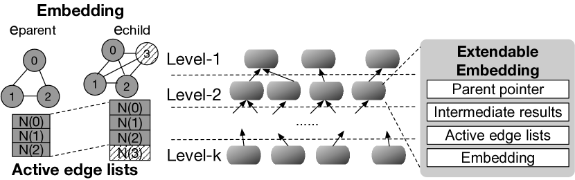
Figure 8. Vertical Data Reuse

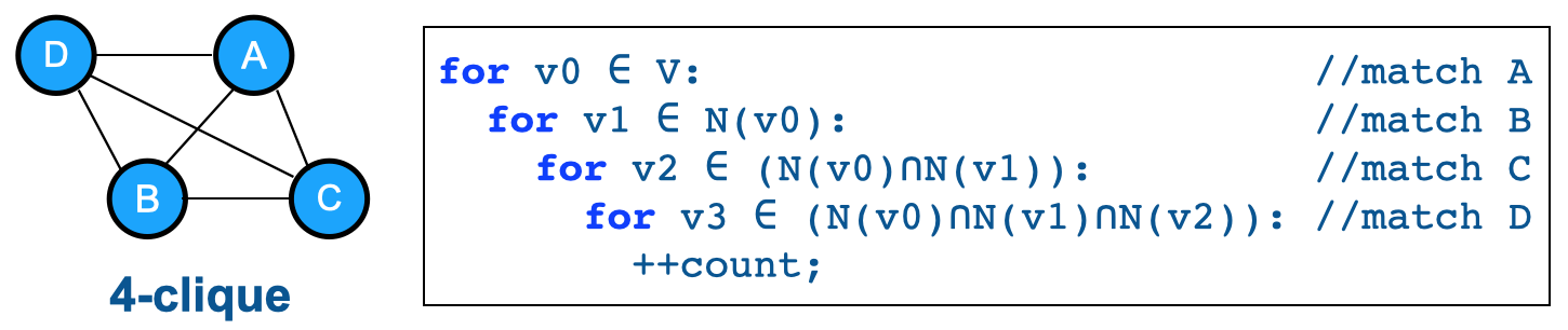
Figure 9. Vertical Computation Reuse

Extending an embedding $e$ may generate intermediate results that can be reused by its descendants to avoid computation redundancy (Mawhirter and Wu, 2019). For 4-clique mining, shown in Figure 9, to extend an edge embedding $e_{edge}=(v_{0},v_{1})$ to a triangle $e_{triangle}$, we should find the common neighbors of $v_{0}$ and $v_{1}$, i.e., calculating $N(v_{0})\cap N(v_{1})$. To further extend the triangle embedding $e_{triangle}=(v_{0},v_{1},v_{2})$ to a 4-clique, we need to find those directly connected with $v_{0}$, $v_{1}$, and $v_{2}$, i.e., calculating $N(v_{0})\cap N(v_{1})\cap N(v_{2})$. In this case, extending $e_{triangle}$ can reuse the intermediate result $N(v_{0})\cap N(v_{1})$ of its parent $e_{edge}$ to avoid extra intersection cost. The hierarchical data representation for vertical data reuse can naturally enable intermediate result sharing between parent and child extendable embedding. The intermediate results that can be shared across levels are determined by algorithm and can be indicated in the EXTEND function. These results are stored in an extendable embedding, its children can directly access them and copy them to its own embedding object. In this way, such intermediate results can be accessed by all descendants.

5.2. Horizontal Data Sharing

The extendable embeddings in the same chunk share the edge lists. If any of them is fetched from remote machines, that should be only done once. We maintain the active edge list of $v$ requested by extendable embeddings $e$ in a chunk in a per-level hash table with $v$ as the key and $e$ as the value. When an extendable embedding $e$ requesting a new active edge list of $v$ (not in $e$’s parent), we first check whether there is already an entry for $v$ in the hash table. If so (suppose the value is $e^{\prime}$), we add an extra pointer in $e$ to $e^{\prime}$, indicating that the new active edge list requested by $e$ can be found in $e^{\prime}$. There is no need to fetch or allocate memory for it. Otherwise, the pointer of $e$ is added to the hash table using $v$ as the key.

To minimize the computation cost, we do not support collisions for hash table insertion—if the hash table entry $hash(v)$ is already occupied by another vertex $u$ with the same hash value, we simply drop the insertion of $v$ rather than building up a collision chain. This simple policy leaves a small amount of redundant communication (or additional memory) that would have been eliminated (or saved) but significantly reduce hash table overhead. We find that the simple design can still drastically reduce the communication cost. For instance, it reduces the communication volume from 4.4TB to 33.8GB for 5-clique mining on the LiveJournal (Leskovec et al., 2009) graph.

5.3. Static Data Cache

Data accesses in GPM show long-term locality. Due to the power law and skewness of graphs, the graph data (edge list) of some vertices are much more frequently accessed than others, and therefore contribute to a large portion of communication cost. For example, the most frequently accessed 5% graph data for 3-motif mining on the UK (Boldi and Vigna, 2004) graph contribute to 93% communication. These “hot-spot” vertices with higher degree are included in more embeddings during the enumeration.

We design an efficient static software graph data cache shared by all chunks, across different chunks at different levels. The cache size is typically 5%-15% of the graph size per node. The cache is empty at the beginning. During embedding enumeration, every time the system is about to fetch the graph data of a vertex $v$, it will query the cache first to see whether the data of $v$ has been cached. If so, it directly obtains the data from it. Otherwise, if $v$’s degree is larger than a threshold (e.g., 64) and the cache is not full, the system will cache $v$’s data after fetching it through the network. Once the cache is full, the system will no longer insert any data to it since we do not support cache eviction and replacement.

We make this design choice to make the cache as lightweight as possible. Our “first accessed first cached with threshold” policy approximately caches the most frequent data—effectively capturing the skewed graph access characteristics. The no replacement policy works well for the following reason. Assuming that graph data accesses are temporally uniformly distributed, if a vertex $v$ is more frequently accessed than $u$ in the whole access history, it is also more likely that the first access to $v$ is earlier than that of $u$. Thus, the more frequently accessed data have higher chance to be placed in the cache.

5.4. NUMA-aware Support

Modern clusters usually adopt the NUMA architecture (Lameter, 2013)—the memory and processors are distributed to multiple sockets, and accessing remote-socket memory is more expensive. To reduce and hide the cost of cross-socket accesses, the graph partition of a $M$-socket node is further divided into $M$ sub-partitions, and each of them is assigned to one socket. We run the BFS-DFS hybrid exploration independently on each socket based on the local sub-partition, which enables circulant scheduling to hide the cost of accesses across both sub-partitions and partitions. Similarly, static data cache is also uniformly divided into $M$ partitions and distributed to each socket. The cache partition on each socket is allowed to cache the graph data residing on a remote socket of the same node, in addition to remote node, and hence reduces cross-socket accesses.

6. Implementation

Kudu engine is implemented in C++ and has approximately 5000 lines of code. We implemented two scalable distributed GPM systems based on partitioned graph, k-Automine and k-GraphPi, by porting two single-machine systems Automine (Mawhirter and Wu, 2019) and GraphPi (Shi et al., 2020) (in its single-node mode) on Kudu, both of which are state-of-the-art systems. GraphPi supports distributed execution with replicated graph, which is compared with k-GraphPi. The porting effort is roughly 500 lines of codes per system, which is significantly less than building a new system from scratch. Since Automine is not open-sourced, k-Automine is modified from our own Automine implementation AutomineIH (in house) that achieves comparable performance with the published results.

Multi-threading support. We leverage multiple computation threads to extend the embeddings in a chunk. The workload is distributed dynamically. Once a batch of extendable embeddings become ready (Section 4.3), they are divided into multiple mini-batches that are the basic workload distribution units (64 embeddings per mini-batch). Mini-batches are added to a lock-free workload queue and distributed to computation threads on demand. Embedding extension generates new extendable embeddings that are inserted to the next-level chunk. We protect the insertion by a mutex. To avoid lock contention, each computation thread has a small local buffer (the size is a half of the L1-D cache) containing the generated embeddings. Once the buffer is full, the embeddings are flushed to the next-level chunk.

Communication subsystem. The communication subsystem is built on top of MPI. It consists of graph data requesting threads and responding threads (ratio $1:1$). The ratio between communication threads and computation threads is $1:3$. Each communication thread runs on a dedicated CPU core to avoid thread scheduling overhead.

7. Evaluation

7.1. Evaluation Methodology

Configuration. Unless otherwise specified, our experiment environment is an 8-node cluster with a 56Gbps InfiniBand network. Each node has two 8-core Intel Xeon E5-2630 v3 CPUs (one CPU per socket) and 64GB DDR4 RAM. The MPI library is OpenMPI 3.0.1.

Graph	Abbr.	—V—	—E—	Max.Degree	Size
MiCo (Elseidy et al., 2014)	mc	96.6K	1.1M	1.4K	9.1MB
Patents (Leskovec et al., 2005)	pt	3.8M	16.5M	0.8K	154.9MB
LiveJournal (Leskovec et al., 2009)	lj	4.8M	42.9M	20.3K	363.9MB
UK-2005 (Boldi and Vigna, 2004)	uk	39.5M	0.94B	1.8M	7.3GB
Twitter-2010 (Kwak et al., 2010)	tw	41.7M	1.5B	3.0M	11.5GB
Friendster (Yang and Leskovec, 2015)	fr	65.6M	1.8B	5.2K	13.9GB
Clueweb12 (Callan, 2012)	cl	978.4M	42.6B	75.6M	324.7GB
UK-2014 (Boldi and Vigna, 2004; Boldi et al., 2011, 2004)	uk14	787.8M	47.6B	8.6M	360.5GB
WDC12 (Meusel et al., 2012)	wdc	3.5B	128.7B	95.0M	984.9GB

Table 1. Graph Datasets (Leskovec and Krevl, 2014)

Datasets. Table 1 shows the evaluated datasets, including three small-size graphs (mc-lj), three median-size datasets (uk-fr), and three large networks (cl-wdc). GPM applications take undirected graphs as input, for directed datasets, the edge direction is simply ignored. All datasets are pre-processed to delete self-loops and duplicated edges.

Evaluated applications. We use four categories of GPM applications. Triangle Counting (TC) is a task that counts the number of triangle. $k$-Motif Counting ($k$-MC) discovers the embeddings for all size-$k$ patterns. $k$-Clique Counting ($k$-CC) counts the number of embeddings of the $k$-clique pattern (a complete graph with $k$ vertices). Frequent Subgraph Mining (FSM) finds all labeled patterns whose supports (i.e., frequencies) (Bringmann and Nijssen, 2008) are no lower than a user-specified threshold.

7.2. Overall Performance

Comparing with distributed systems. We first compare Kudu based systems (k-Automine and k-GraphPi) with G-thinker (Yan et al., 2020), the only state-of-the-art distributed GPM system with partitioned graph. The results are presented in Table 2. We notice that G-thinker’s performance is very low with two sockets per node due to its lack of NUMA support. Hence, we also report the single-socket runtimes of G-thinker/k-Automine/k-GraphPi in parentheses and use them to calculate speedups. k-Automine and k-GraphPi on average outperform G-thinker by $17.7\times$ and $20.3\times$ (up to $75.5\times$ and $75.5\times$), respectively. The speedup on Patents graph is very high because it is less-skewed. In G-thinker, the cache management overhead cannot be effective amortized by graph data accessing time, leading to quite low performance.

Next, we compare our systems with GraphPi (Shi et al., 2020), the fastest distributed GPM systems based on replicated graph (Table 2). Surprisingly, except for 5-CC on MiCo, k-GraphPi consistently delivers better performance than GraphPi even with the remote graph accessing overhead. The performance improvement is attributed to two reasons: 1) GraphPi’s implementation adopts a complicated task partitioning and distribution method that leads to large overhead, and hence is slower on small-size workloads; 2) By decomposing the subgraph enumeration process into fine-grained embedding extension tasks, Kudu can exploit strictly more parallelism than GraphPi that only parallelizes the first or first few loops of the subgraph enumeration process in a coarse-grained fashion. For 3-MC, k-Automine is slower than k-GraphPi because of GraphPi’s better pattern matching algorithm.

App.	G.	k-Automine	k-GraphPi	GraphPi	G-thinker
		(partitioned)	(partitioned)	(replicated)	(partitioned)
#nodes		8	8	8	8
TC	mc	40.2ms (34.5ms)	35.3ms (35.0ms)	704.4ms	2.2s (1.2s)
	pt	221.2ms (361.1ms)	225.0ms (363.9ms)	6.7s	124.7s (27.2s)
	lj	706.8ms (1.2s)	722.4ms (1.2s)	9.8s	904.9s (34.6s)
	uk	705.5s	706.2s	1268.4s	CRASHED
	tw	2293.1s	2300.6s	2886.5s	CRASHED
	fr	84.1s	78.5s	169.2s	CRASHED
3-MC	mc	57.6ms (67.8ms)	56.4ms (44.6ms)	1.5s	2.2s (1.2s)
	pt	363.1ms (642.1ms)	289.2ms (459.1ms)	13.8s	34.6s (27.5s)
	lj	1.6s (3.0s)	847.3ms (1.4s)	20.1s	215.5s (36.7s)
	uk	1.1h	689.4s	1,380.7s	CRASHED
	tw	2.8h	2309.9s	3,032.1s	CRASHED
	fr	194.0s	82.4s	388.5s	CRASHED
4-CC	mc	293.8ms (485.0ms)	299.9ms (478.8ms)	844.0ms	2.2s (2.3s)
	pt	370.2ms (627.7ms)	362.8ms (606.0ms)	6.7s	35.7s (26.5s)
	lj	4.7s (8.6s)	4.8s (8.7s)	12.8s	89.1s (37.7s)
	uk	5.1h	5.1h	8.6h	CRASHED
	tw	6.7h	6.8h	TIMEOUT	CRASHED
	fr	132.9s	137.7s	177.8s	CRASHED
5-CC	mc	9.8s (16.0s)	9.9s (16.1s)	8.2s	52.5s (52.1s)
	pt	780.7ms (985.7ms)	777.6ms (994.5ms)	6.8s	37.5s (27.6s)
	lj	169.6s	169.3s	174.7s	CRASHED
	fr	204.3s	210.3s	260.0s	CRASHED

Table 2. Comparing with GraphPi/G-thinker (Timeout: 10h); Runtimes with one socket per node shown in parentheses

App.	Graph	k-Automine	AutomineIH	Peregrine	Pangolin
#nodes		1	1	1	1
TC	mc	83.5ms	52.3ms	68.7ms	56ms
	pt	1.2s	330.7ms	1.1s	289ms
	lj	4.6s	2.8s	3.8s	2.2s
	uk	1.7h	2.0h	1.3h	26.6s
	tw	4.7h	8.6h	5.7h	747.7s
	fr	497.2s	378.3s	305.2s	384.6s
3-MC	mc	222.9ms	160.3ms	84.7ms	288ms
	pt	2.3s	930.9ms	1.7s	1.5s
	lj	12.0s	8.9s	4.6s	29.2s
	uk	9.1h	TIMEOUT	1.3h	TIMEOUT
	fr	1425.8s	1206.8s	316.1s	1.8h
4-CC	mc	1.7s	1.2s	1.8s	2.8s
	pt	2.0s	381.0ms	1.3s	773ms
	lj	32.3s	31.3s	49.6s	54.7s
	fr	852.6s	570.3s	1237.5s	OUTOFMEM
5-CC	mc	66.1s	46.8s	78.0s	132.0s
	pt	3.4s	408.4ms	1.5s	967ms
	lj	1259.3s	982.9s	2076.6s	OUTOFMEM
	fr	1435.1s	900.2s	3032.8s	OUTOFMEM

Table 3. Comparing with Single-machine Systems

Comparing with single-machine systems. To show the efficiency of Kudu, we further compare k-Automine’s single-node performance with three state-of-the-art single-machine systems and report the results in Table 3. We see that k-Automine achieves comparable performance with the baselines for most workloads. It is even faster than AutomineIH for TC/3-MC on the uk and tw graphs because of Kudu’s fine-grained parallelism. On the other side, k-Automine is less effcient on pt. We analyze the inefficiency on pt in Section 7.5. Pangolin is extremely fast for TC on the uk and tw graphs because of orientation (Chen et al., 2020), a powerful algorithmic optimization specifically targeting triangle and clique counting on skewed graphs, which is not adopted by Automine or Peregrine. This optimization can be easily integrated into Kudu as a pre-processing step. We do not enable the optimization here for fair comparisons with Automine and Peregrine.

Comparing with graph-query systems. We also compares our systems with aDFS in Figure 10. Since aDFS is not open-sourced, we compares to the TC runtimes reported in their paper (Trigonakis et al., 2021) on the Skitter (Leskovec et al., 2005), Orkut (Yang and Leskovec, 2015), and Friendster (Yang and Leskovec, 2015) graphs measured on a cluster with eight 28-core nodes. Although with less computation resources (128 cores), k-Automine and k-GraphPi significantly outperforms aDFS by up to one order of magnitude thanks to our better “move data to computation” policy.

Figure 10. Comparing with aDFS

FSM performance. We ran k-Automine on both single-node and distributed modes on mc, pt, and lj graphs, and compared it with two single-node systems (Peregrine and AutomineIH) and a distributed system with 8-node (Fractal (Dias et al., 2019)). We do not evaluate k-GraphPi or GraphPi since GraphPi does not come with a reference FSM implementation. Similar to the Peregrine paper (Jamshidi et al., 2020), we only discover frequent patterns with no more than three edges. Note that FSM requires labeled graphs. Hence, for unlabeled datasets like lj, we randomly synthesized their labels. The results are shown in Table 4. k-Automine running in the single-node mode is consistently slower than AutomineIH. The reason is that FSM processes a large number of candidate labeled patterns, and hence the per-pattern startup overhead of Kudu (i.e., initializing the embedding execution engine) becomes non-negligible. k-Automine running on 8 nodes is significantly faster than AutomineIH/Peregrine with one node and Fractal with 8 nodes thanks to its ability to leverage the cluster-wide computation resource efficiently.

Graph	Threshold	k-Automine		AutomineIH	Peregrine	Fractal
#Nodes		1	8	1	1	8
mc	3K	91.1s	18.8s	46.7s	181.3s	105.1s
	4K	90.1s	15.6s	45.3s	170.6s	102.1s
	5K	89.7s	15.2s	45.1s	166.9s	108.3s
pt	13K	288.9s	44.0s	103.4s	256.1s	301.7s
	14K	288.3s	44.1s	104.2s	255.1s	302.6s
	15K	288.1s	44.1s	103.7s	257.2s	347.6s
lj	800K	TIMEOUT	1.9h	TIMEOUT	TIMEOUT	TIMEOUT
	900K	6.3h	0.8h	5.7h	TIMEOUT	TIMEOUT
	1M	6.3h	0.8h	5.7h	TIMEOUT	TIMEOUT

Table 4. FSM Performance

Performance on large-scale graphs. We study Kudu’s scalability to large graphs by running k-Automine on three massive datasets (cl, uk14, wdc) for TC and 4-CC. To the best of our knowledge, wdc is the largest publicly available real-world graph with more than 3 billion vertices and 128 billion edges. k-Automine is evaluated on an 18-node cluster (two 16-core Intel Xeon-6130 CPUs and 128GB RAM each node). Note that all of the three graphs cannot fit in the memory of a single node (128GB), and hence cannot be processed by graph replication based systems like GraphPi. For comparison purposes, we run AutomineIH for the same workloads on a high-end 64-core machine with two AMD Epyc-7513 CPUs and 1TB memory. We adopt the triangle/clique-specific orientation optimization  (Chen et al., 2020) mentioned previously, which converts the undirected input graph to a directed acyclic graph (DAG) as a pre-processing step to reduce the computation cost for both k-Automine and AutomineIH. The results are presented in Table 5. k-Automine significantly outperforms AutomineIH in all cases by up to $4.5\times$ ($3.2\times$ on average) thanks to Kudu’s ability to leverage a larger amount of cluster-wide computation resources. With graph partitioning, Kudu can efficiently scale to massive graphs that requires the memory and computation resources beyond the capacity of a single machine. More impressively, k-Automine even outperforms a state-of-the-art CPU-based distributed triangle counting implementation (Pearce, 2017) (with the orientation optimization) targeting large graphs, which counts all 9.65 trillion triangles of the wdc graph with 808.7 seconds using 256 24-core machines (in total 6144 cores). By contrast, k-Automine finished triangle counting on wdc with 200.5 seconds, achieving $4.0\times$ speedups with only $9.4\%$ of its computation resource (576 cores).

Graph	#Vertices / #Edges	App	k-Automine	AutomineIH
cl	1.0B / 42.6B	TC	53.8s	115.1s
		4-CC	0.75h	2.6h
uk14	0.8B / 47.6B	TC	94.1s	299.4s
		4-CC	16.0h	72.2h
wdc	3.5B / 128.7B	TC	200.5s	560.81s
		4-CC	18.8h	66.5h

Table 5. Kudu’s Performance on Large-Scale Graphs

7.3. Analyzing Kudu Optimizations

Vertical computation sharing (VCS). We run k-GraphPi for 4-CC and 5-CC with/without the optimization, and report

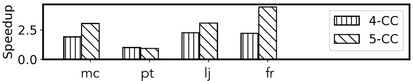
Figure 11. Speedup by VCS

the speedups in Figure 11. The optimization improves the performance by $2.10\times$ on average (up to $4.44\times$). It is not very effective on the pt graph since as mentioned earlier, embedding extension is lightweight on pt and only takes a small portion of execution time.

Horizontal data sharing. We analyze the effect of horizontal data sharing (HDS) by running k-GraphPi for 4-CC and

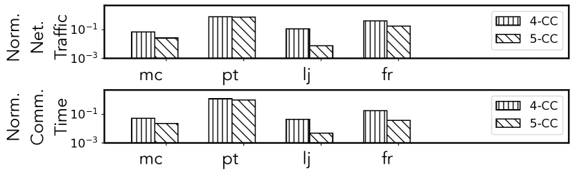
Figure 12. Effect of HDS

5-CC with/without the optimization. We report the network traffic and communication time (normalized with respect to the version without the optimization) on critical path in Figure 12. The optimization reduces network traffic and critical-path communication time by 70.5% and 67.8% on average (up to 99.3% and 99.5%), respectively. The traffic reduction is moderate on the pt graph (20.4% for 4-CC and 24.3% for 5-CC). It is because pt is less-skewed and thus there are less “hot-spot’ active vertices appearing multiple times within a chunk.

App.	G.	Network Traffic		Runtime
		with cache	no cache	with cache	no cache
TC	pt	962.1MB	1.0GB	225.0ms	228.5ms
	lj	6.8GB	7.9GB	722.4ms	770.8ms
	uk	487.3GB	57.7TB	706.2s	2615.2s
	fr	1.4TB	1.8TB	78.5s	89.6s
4-CC	pt	1.2GB	1.6GB	362.8ms	412.7ms
	lj	15.7GB	25.2GB	4.8s	4.9s
	fr	2.3TB	3.2TB	137.7s	185.3s
5-CC	pt	1.3GB	1.8GB	777.6ms	795.1ms
	lj	33.8GB	86.6GB	169.3s	169.5s
	fr	2.7TB	3.7TB	210.3s	250.1s

Table 6. Analyzing the Static Data Cache (k-GraphPi)

Static data cache. The effect of static data cache is reported in Table 6. The optimization significantly reduces network traffic and hence improves end-to-end performance. The optimization is extremely useful for highly-skewed graphs like uk. For TC on uk, it reduces the traffic from 57.7TB to 487.3GB by more than 99% (even with other optimizations like horizontal data sharing), and improves performance by $3.7\times$. Reduction in network traffic does not necessarily translate to performance benefit (e.g., 4-CC on lj) since communication cost is already completely hidden by computation.

App.	Graph	With NUMA support	No NUMA support
4-CC	pt	2.1s (1.53x)	3.2s
	lj	33.0s (1.20x)	39.5s
	fr	870.4s (1.15x)	998.5s
5-CC	pt	4.0s (1.47x)	5.9s
	lj	1243.2s (1.02x)	1269.5s
	fr	1487.6s (1.30x)	1930.7s

Table 7. NUMA-aware Support

NUMA-aware support. We analyze our NUMA-aware support by running k-GraphPi on a single node. Table 7 shows that Kudu’s NUMA awareness leads to on average $1.26\times$ (up to $1.53\times$) performance gain.

7.4. Scalability

Inter-node scalability. We report inter-node scalability of k-GraphPi and GraphPi in Figure 13 by varying the number of nodes. k-GraphPi achieves similar or even better scalability compared with GraphPi, and scales almost perfectly. Leveraging 8 nodes is on average $6.77\times$ (up to $7.35\times$) faster than one node. By contrast, GraphPi’s speedup is on average $4.04\times$.

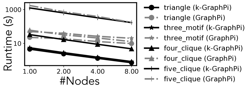
Figure 13. Kudu’s Inter-node Scalability (graph: lj)

Intra-node scalability and the COST metric. In Figure 14, we analyze Kudu’s intra-node scalability and efficiency by running k-Automine on a single node using different numbers of CPU cores (5,

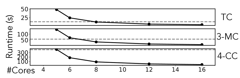
Figure 14. Intra-node Scalability

6, 8, 12, 16) on graph lj. The number of cores starts from five since four cores are always reserved for communication threads. By utilizing 16 cores, k-Automine achieves $10.7\times$, $11.6\times$ and $11.4\times$ speedups for TC, 3-MC and 4-CC on the lj graph, respectively. We also report the COST metric—the number of cores with which a distributed system can outperform an efficient reference single-thread implementation (McSherry et al., 2015). We use the fastest single-thread runtime among Automine, Peregrine and Pangolin as the reference single-thread runtime (the dotted line in Figure 14). The COST metrics for TC, 3-MC and 4-CC are 8, 8, 6, respectively.

7.5. Execution Time Breakdown

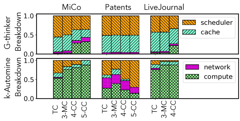
Figure 15. Runtime breakdown of G-thinker/k-Automine

We compare the runtime breakdown of G-thinker and k-Automine in Figure 15. There are missing data points (e.g., 5-CC on lj) since G-thinker crashes due to an internal bug. For G-thinker, most runtime is spent on cache maintaining (“cache”) (41.03% on average) and scheduling (“scheduler”) (45.49% on average). Only a small portion of time is spent on communication (“network”) (4.66% on average) and embedding tree exploration (“compute”) (8.82% on average). By contrast, k-Automine significantly increases the portion of “compute” to 59.48% on average (up to 88.24%) thanks to our lightweight design. We also notice that except for Patents, the communication overhead of k-Automine is very low (less than 5%), indicating the effectiveness of our communication optimizations. The “scheduler” and “network” on Patents are still high (45.09% and 22.70% on average). Patents is a less-skewed graph with low max-degree whose subgraph extension tasks are lightweight. Hence, the computation is not sufficient to amortize the scheduling overhead or hide the communication cost.

7.6. Cache Design Analysis

Effects of cache policies. As shown in Figure 16, we evaluate different cache replacement policies, including FIFO (first-in-first-out), LIFO (last-in-first-out), LRU (least-recently-used), MRU (most-recently-used) and STATIC (no-replacement) and report the volume of network traffic and execution time. Both traffics and runtimes are normalized w.r.t. the STATIC policy. In terms of traffic volume, STATIC is similar or slightly better than LIFO and MRU but worse than FIFO and LRU on three workloads (5-CC on lj and 4-CC/5-CC on fr). It is because of STATIC’s inability to capture the temporal change in data access pattern during execution—not a very surprising result because of its simple no-replacement design. However, interestingly, more communication traffic on these workloads does not result in performance degeneration. We observed that in all cases, STATIC beats other policies by roughly one order of magnitude in terms of performance.

The reason is twofold. On the one hand, as shown in Figure 15, communication is no longer a major bottleneck even with the suboptimal STATIC policy. Further reducing the communication with a sophisticated policy is less beneficial as it has passed the point of diminishing returns. On the other hand, policies with replacement incur more computation cost. First, they have to maintain/update the cache during the whole execution while STATIC only needs to fill up the cache at the beginning of execution, completely eliminating the update cost after the cache is full. Second, memory management is more complicated for policies with replacement. Note that the cached vertices have various degrees and need different sizes of memory blocks to store the graph data. Hence, allocating/de-allocating the memory of a newly cached/uncached vertex cannot be done via a fast fix-size memory pool but requires a general-purpose dynamic memory allocator (e.g., UNIX malloc/free). Long-term frequent irregular memory allocation/de-allocation/re-allocation cause the fragmentation problem, significantly increasing the memory management cost. In contrast, STATIC only needs allocations and thus avoids the fragmentation, making its memory management much faster.

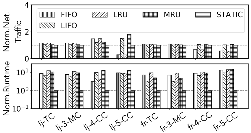
Figure 16. Comparing Different Cache Policies (k-GraphPi)

Effects of cache size. We evaluated k-GraphPi’s performance with different cache sizes, varying from 1%-50% of the graph size, and reported the network traffic volumes, cache hit rates, and execution times in Figure 17. The traffic volumes and runtimes are normalized w.r.t. the cases when the cache size is 1% of the graph size. As the cache size increases, the runtime and traffic mostly decrease and the cache hit rate gets higher. There is a point of diminishing returns where performance stops growing even with a larger cache (e.g., 10% for uk-TC and 30% for fr-4-CC) as communication can be completely hidden with computation. It is worth noting that the runtimes of lj-TC and lj-3-MC increase slightly (by 6-8%) when the cache size increases to 50%. It is because of the effect of the hardware CPU cache. When the software cache size is small, it can be completely kept in the CPU L3 cache, leading to low software-cache update/query overhead. As the size of the software cache grows, it exceeds the size of L3 cache, incurring higher update/query cost and hence affect the overall performance.

Although a larger cache can lead to higher performance, it affects the scalability to massive graphs: if the single-node memory is 64GB and the cache size is set to 50% of the graph size, the system can only support graphs up to 128GB. To achieve a good tradeoff between performance and scalabiltiy, we limit the cache size to be at most 15% of the graph size for regular-size datasets and further reduce it to 3-4% for massive datasets like WDC12.

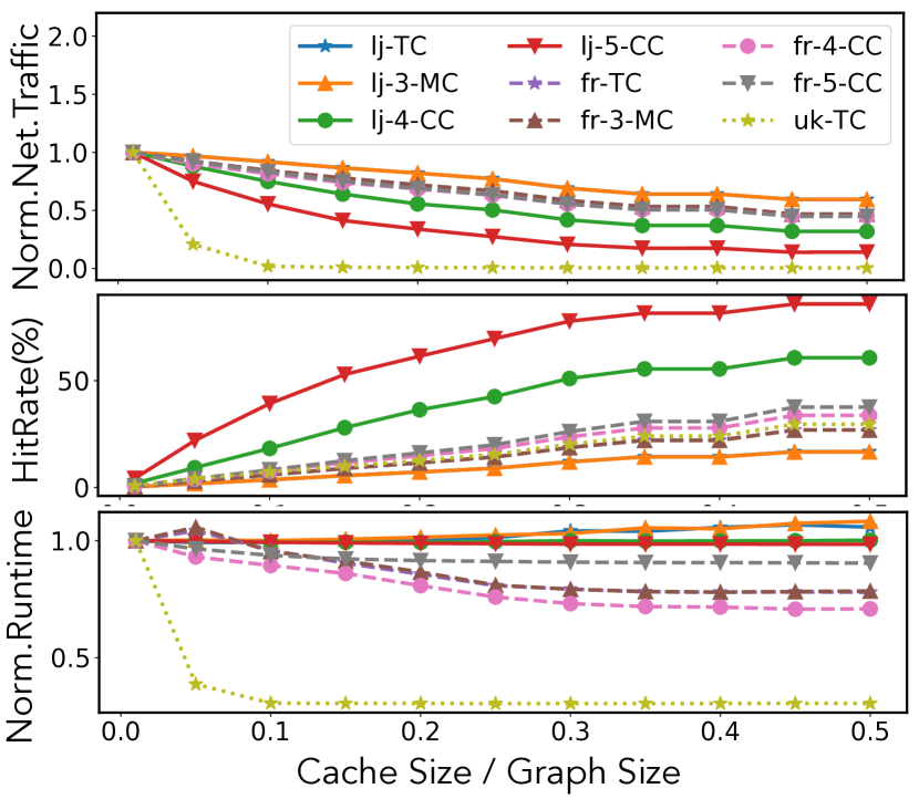
Figure 17. Varying Cache Size (k-GraphPi)

7.7. Sensitivity Tests on Chunk Size

We evaluate the performance with various chunk sizes (from 1MB to 16GB) in the hybrid exploration as shown in Figure 18. The runtime decreases as the chunk size increases because of 1) more parallelism; 2) more opportunities to reuse data within a chunk. We empirically choose chunk size to be 4GB by default since it maximizes the performance while not introducing too much memory overhead (at most 4GB$\times$(5-1)=16GB for 5-CC). It is worth pointing out that the memory overhead is fixed regardless of graph size and will not affect the scalability. In general, the results suggest that the larger chunk is helpful, as long as the memory of the machine is sufficient.

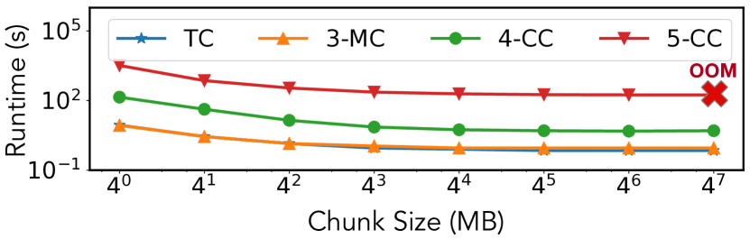
Figure 18. Varying Chunk Size (k-GraphPi, lj graph)

7.8. Network Utilization

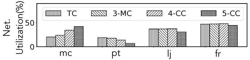
Figure 19. Network Bandwidth Utilization (k-GraphPi)

The network bandwidth utilization is shown in Figure 19. The system is compute-bounded on most workloads and thus network bandwidth is not saturated. For most cases, the communication threads become idle to wait for more requests from computation threads. The only exception is the Patents graph, in which the communication thread serving data requests spent most of the time copying data from the local graph partition to a communication buffer so that they can be sent in a batch back to the requesting node. As a result, the network is largely underutilized. It is because most requests only access a small amount of data and have memory poor locality.

8. Conclusion

This paper proposes Kudu, a distributed execution engine that can be integrated with existing single-machine graph pattern mining (GPM) systems. The key novelty is the extendable embedding abstraction which can express pattern enumeration algorithms, enable fine-grained task scheduling, enable low-cost GPM-specific data reuse. Two scalable distributed GPM systems are implemented by porting Automine and GraphPi on Kudu. Our evaluation shows that Kudu based systems significantly outperform state-of-the-art distributed GPM systems with graph partitioning by up to $75.5\times$, achieve similar or even better performance compared with the fastest graph replication based system, and scale to massive graphs with more than one hundred billion edges.

References

- (1)
- Becchetti et al. (2008) Luca Becchetti, Paolo Boldi, Carlos Castillo, and Aristides Gionis. 2008. Efficient semi-streaming algorithms for local triangle counting in massive graphs. In Proceedings of the 14th ACM SIGKDD international conference on Knowledge discovery and data mining. 16–24.
- Bindschaedler et al. (2021) Laurent Bindschaedler, Jasmina Malicevic, Baptiste Lepers, Ashvin Goel, and Willy Zwaenepoel. 2021. Tesseract: distributed, general graph pattern mining on evolving graphs. In Proceedings of the Sixteenth European Conference on Computer Systems. 458–473.
- Boldi et al. (2004) Paolo Boldi, Bruno Codenotti, Massimo Santini, and Sebastiano Vigna. 2004. Ubicrawler: A scalable fully distributed web crawler. Software: Practice and Experience 34, 8 (2004), 711–726.
- Boldi et al. (2011) Paolo Boldi, Marco Rosa, Massimo Santini, and Sebastiano Vigna. 2011. Layered label propagation: A multiresolution coordinate-free ordering for compressing social networks. In Proceedings of the 20th international conference on World wide web. 587–596.
- Boldi and Vigna (2004) Paolo Boldi and Sebastiano Vigna. 2004. The webgraph framework I: compression techniques. In Proceedings of the 13th international conference on World Wide Web. 595–602.
- Bringmann and Nijssen (2008) Björn Bringmann and Siegfried Nijssen. 2008. What is frequent in a single graph?. In Pacific-Asia Conference on Knowledge Discovery and Data Mining. Springer, 858–863.
- Callan (2012) Jamie Callan. 2012. The lemur project and its ClueWeb12 dataset. In Invited talk at the SIGIR 2012 Workshop on Open-Source Information Retrieval.
- Chen et al. (2018) Hongzhi Chen, Miao Liu, Yunjian Zhao, Xiao Yan, Da Yan, and James Cheng. 2018. G-Miner: an efficient task-oriented graph mining system. In Proceedings of the Thirteenth EuroSys Conference. 1–12.
- Chen et al. (2021) Xuhao Chen, Roshan Dathathri, Gurbinder Gill, Loc Hoang, and Keshav Pingali. 2021. Sandslash: a two-level framework for efficient graph pattern mining. In Proceedings of the ACM International Conference on Supercomputing. 378–391.
- Chen et al. (2020) Xuhao Chen, Roshan Dathathri, Gurbinder Gill, and Keshav Pingali. 2020. Pangolin: an efficient and flexible graph mining system on CPU and GPU. Proceedings of the VLDB Endowment 13, 10 (2020), 1190–1205.
- Dias et al. (2019) Vinicius Dias, Carlos HC Teixeira, Dorgival Guedes, Wagner Meira, and Srinivasan Parthasarathy. 2019. Fractal: A general-purpose graph pattern mining system. In Proceedings of the 2019 International Conference on Management of Data. 1357–1374.
- Elseidy et al. (2014) Mohammed Elseidy, Ehab Abdelhamid, Spiros Skiadopoulos, and Panos Kalnis. 2014. Grami: Frequent subgraph and pattern mining in a single large graph. Proceedings of the VLDB Endowment 7, 7 (2014), 517–528.
- Jamshidi et al. (2020) Kasra Jamshidi, Rakesh Mahadasa, and Keval Vora. 2020. Peregrine: a pattern-aware graph mining system. In Proceedings of the Fifteenth European Conference on Computer Systems. 1–16.
- Juszczyszyn and Kołaczek (2011) Krzysztof Juszczyszyn and Grzegorz Kołaczek. 2011. Motif-based attack detection in network communication graphs. In IFIP International Conference on Communications and Multimedia Security. Springer, 206–213.
- Kwak et al. (2010) Haewoon Kwak, Changhyun Lee, Hosung Park, and Sue Moon. 2010. What is Twitter, a social network or a news media?. In Proceedings of the 19th international conference on World wide web. 591–600.
- Lameter (2013) Christoph Lameter. 2013. An overview of non-uniform memory access. Commun. ACM 56, 9 (2013), 59–54.
- Leskovec et al. (2010) Jure Leskovec, Daniel Huttenlocher, and Jon Kleinberg. 2010. Signed networks in social media. In Proceedings of the SIGCHI conference on human factors in computing systems. 1361–1370.
- Leskovec et al. (2005) Jure Leskovec, Jon Kleinberg, and Christos Faloutsos. 2005. Graphs over time: densification laws, shrinking diameters and possible explanations. In Proceedings of the eleventh ACM SIGKDD international conference on Knowledge discovery in data mining. 177–187.
- Leskovec and Krevl (2014) Jure Leskovec and Andrej Krevl. 2014. SNAP Datasets: Stanford Large Network Dataset Collection. http://snap.stanford.edu/data.
- Leskovec et al. (2009) Jure Leskovec, Kevin J Lang, Anirban Dasgupta, and Michael W Mahoney. 2009. Community structure in large networks: Natural cluster sizes and the absence of large well-defined clusters. Internet Mathematics 6, 1 (2009), 29–123.
- Ma’ayan (2009) Avi Ma’ayan. 2009. Insights into the organization of biochemical regulatory networks using graph theory analyses. Journal of Biological Chemistry 284, 9 (2009), 5451–5455.
- Malewicz et al. (2010) Grzegorz Malewicz, Matthew H Austern, Aart JC Bik, James C Dehnert, Ilan Horn, Naty Leiser, and Grzegorz Czajkowski. 2010. Pregel: a system for large-scale graph processing. In Proceedings of the 2010 ACM SIGMOD International Conference on Management of data. 135–146.
- Mawhirter et al. (2021) Daniel Mawhirter, Sam Reinehr, Connor Holmes, Tongping Liu, and Bo Wu. 2021. GraphZero: A High-Performance Subgraph Matching System. ACM SIGOPS Operating Systems Review 55, 1 (2021), 21–37.
- Mawhirter and Wu (2019) Daniel Mawhirter and Bo Wu. 2019. AutoMine: harmonizing high-level abstraction and high performance for graph mining. In Proceedings of the 27th ACM Symposium on Operating Systems Principles. 509–523.
- McSherry et al. (2015) Frank McSherry, Michael Isard, and Derek G Murray. 2015. Scalability! But at what COST?. In 15th Workshop on Hot Topics in Operating Systems (HotOS XV).
- Meusel et al. (2012) Robert Meusel, Sebastiano Vigna, Oliver Lehmberg, and Christian Bizer. 2012. Web data commons-hyperlink graphs. URL http://webdatacommons. org/hyperlinkgraph/index. html (2012).
- Pearce (2017) Roger Pearce. 2017. Triangle counting for scale-free graphs at scale in distributed memory. In 2017 IEEE High Performance Extreme Computing Conference (HPEC). IEEE, 1–4.
- Schmidt et al. (2011) Matthew C Schmidt, Andrea M Rocha, Kanchana Padmanabhan, Zhengzhang Chen, Kathleen Scott, James R Mihelcic, and Nagiza F Samatova. 2011. Efficient , -motif finder for identification of phenotype-related functional modules. BMC bioinformatics 12, 1 (2011), 440.
- Shi et al. (2020) Tianhui Shi, Mingshu Zhai, Yi Xu, and Jidong Zhai. 2020. GraphPi: high performance graph pattern matching through effective redundancy elimination. In Proceedings of the International Conference for High Performance Computing, Networking, Storage and Analysis. 1–14.
- Staniford-Chen et al. (1996) Stuart Staniford-Chen, Steven Cheung, Richard Crawford, Mark Dilger, Jeremy Frank, James Hoagland, Karl Levitt, Christopher Wee, Raymond Yip, and Dan Zerkle. 1996. GrIDS-a graph based intrusion detection system for large networks. In Proceedings of the 19th national information systems security conference, Vol. 1. Baltimore, 361–370.
- Teixeira et al. (2015) Carlos HC Teixeira, Alexandre J Fonseca, Marco Serafini, Georgos Siganos, Mohammed J Zaki, and Ashraf Aboulnaga. 2015. Arabesque: a system for distributed graph mining. In Proceedings of the 25th Symposium on Operating Systems Principles. 425–440.
- Trigonakis et al. (2021) Vasileios Trigonakis, Jean-Pierre Lozi, Tomáš Faltín, Nicholas P Roth, Iraklis Psaroudakis, Arnaud Delamare, Vlad Haprian, Călin Iorgulescu, Petr Koupy, Jinsoo Lee, et al. 2021. aDFS: An Almost Depth-First-Search Distributed Graph-Querying System. In 2021 USENIX Annual Technical Conference (USENIX ATC 21). 209–224.
- Valverde and Solé (2005) Sergi Valverde and Ricard V Solé. 2005. Network motifs in computational graphs: A case study in software architecture. Physical Review E 72, 2 (2005), 026107.
- Wang et al. (2018) Kai Wang, Zhiqiang Zuo, John Thorpe, Tien Quang Nguyen, and Guoqing Harry Xu. 2018. Rstream: Marrying relational algebra with streaming for efficient graph mining on a single machine. In 13th USENIX Symposium on Operating Systems Design and Implementation (OSDI 18). 763–782.
- Wu et al. (2018) Peng Wu, Junfeng Wang, and Bin Tian. 2018. Software homology detection with software motifs based on function-call graph. IEEE Access 6 (2018), 19007–19017.
- Yan et al. (2020) Da Yan, Guimu Guo, Md Mashiur Rahman Chowdhury, M Tamer Özsu, Wei-Shinn Ku, and John CS Lui. 2020. G-thinker: A Distributed Framework for Mining Subgraphs in a Big Graph. In 2020 IEEE 36th International Conference on Data Engineering (ICDE). IEEE, 1369–1380.
- Yang and Leskovec (2015) Jaewon Yang and Jure Leskovec. 2015. Defining and evaluating network communities based on ground-truth. Knowledge and Information Systems 42, 1 (2015), 181–213.